Probing Neural Networks for the Gamma/Hadron Separation of the Cherenkov Telescope Array

Abstract

We compared convolutional neural networks to the classical boosted decision trees for the separation of atmospheric particle showers generated by gamma rays from the particle-induced background. We conduct the comparison of the two techniques applied to simulated observation data from the Cherenkov Telescope Array. We then looked at the Receiver Operating Characteristics (ROC) curves produced by the two approaches and discuss the similarities and differences between both. We found that neural networks overperformed classical techniques under specific conditions.

1 Introduction

Machine learning made spectacular advances during the last few years. Deep convolutional neural networks (CNNs) emerged as a very powerful technique thanks to advances in algorithms, data availability and overall computational power. CNNs recently proved to be effective also for TeV astrophysics [1] to separate the signal from an astronomical source from the cosmic-ray background. The Cherenkov Telescope Array (CTA) [2] will be the next-generation ground-based gamma-ray observatory, composed of more than one-hundred telescopes at two observation sites. Its sensitivity will improve by an order of magnitude compared to existing facilities. Improving the data analysis techniques to better discriminate the observed gamma rays from the cosmic rays would allow to better resolve the observed sources and also to reduce the observation time needed to obtain enough significance.
In this paper we focus on the signal extraction and we evaluate the performance of CNNs compared to Boosted Decision Trees (BDTs) [3] which are commonly used for this task and in particular in the EventDisplay analysis package [4]. Other techniques are commonly employed such as random forests [5] or maximum-likelihood [6]. To perform this comparison, we took the Event parameter output of the EventDisplay analysis of simulated events from a Monte-Carlo (MC) production of CTA. We picked the dataset that contained the most realistic observation conditions and applied CNNs to it. We then compared the obtained Signal/Background separation performances with the one from the BDTs from EventDisplay.

1.1 Cherenkov Astronomy

Cherenkov Astronomy studies very high-energy $\gamma$-ray emission from the Galaxy and beyond. Above a few GeV, the flux from the sources is too small to be detected with a compact instrument. Instead, it relies on the interaction between high-energy gamma rays and the Earth’s atmosphere. These interactions produce showers of particles travelling faster than light in the atmostphere which thus emit Cherenkov light. This light is detected by arrays of large telescopes and very fast cameras. Each individual shower detection is called an event, which combines images seen in coincidence in several telescopes.
Images typically look like elongated ellipses, and these can be combined to give event-level parameters. They can be of several types, namely photonic (gammas), hadronic or electronic. It is the gamma events that are of interest, as hadronic events originate from cosmic-rays. The discrimination of events cannot be fully accurate and thus gamma events are discarded hence reducing the sensitivity of the facility. The opposite also occurs, with many hadronic events being classified as gammas, hence contaminating the measurement with background noise.

1.2 Convolutional Neural Networks

CNNs extract features from images and combine them to derive higher level knowledge. Their architecture has grown more complex over the years, and they now outperform humans in recognizing a large variety of items in images. The current best performing network, called Squeeze-and-Excitation [7] was able to recognize which of the 1000 possible object categories appeared on pictures with an accuracy of 97.75 percents during the 2017 annual ImageNet challenge [8]. This approach started to be applied in astrophysics to separate signal from sources from background noise. [9] used CNNs and generative adversarial networks to recover features in astrophysical images of galaxies beyond the deconvolution limit. CNNs were also used by [10] to deconvolve strongly-lensed images of galaxies. [11] used a similar approach to detect such images while [12] used Generative Adversarial Networks to separate quasar point sources from the light of its host galaxy. [13] used deep-learning to reconstruct air showers from data coming from the Pierre Auger Observatory [14]. Eventually, [15] applied deep learning to gravitational waves detection and the estimation of their parameters using Laser Interferometer Gravitational-Wave Observatory data [16].

2 Proposed method

The performances of neural networks can be quite difficult to evaluate because they are very sensitive to the training and validation datasets that are used. The computer vision community solved this issue by defining a standard dataset to be used both for training and evaluation of new architectures [17]. Such dataset does not yet exist in high-energy astrophysics. Thus, we decided to evaluate the performances of CNNs with respect to what is the current standard in the field, namely BDTs. CTA has produced a standard analysis of the simulated data, and it is against this classification that we evaluated our neural networks. The CTA standard analysis relies on the EventDisplay package [4] that was originally developed for the VERITAS experiment [18]. Another package named MARS [19] is used to crosscheck the results. We used exactly the same datasets for both the BDTs and the neural networks. Both have exactly the same amount of data to work with, hence we believe that such a comparison is fair and makes sense in this context. We did not perform the EventDisplay analysis ourselves as the output of the analysis is available to all CTA consortium members. Both approaches are compared by plotting their Receiver Operating Characteristics (ROC) curves. The Area Under Curve (AUC) is used to assess the methods’ overall performances, while subtle differences between the curves are discussed to make predictions about their true performances.

3 Monte-Carlo Data

We decided to use the datasets from night sky background (NSB) studies to perform this comparison. These datasets are well suited because they were designed to represent the standard operating conditions of CTA. We stick to the standard NSB level as it is the one that is the closest to the expected nominal conditions and used only medium-size telescopes data, as did the BDT analysis. The CTA expert helped us retrieve a list of events that were used to train and validate the BDTs. The datasets contain only diffuse protons and diffuse gammas. No electrons were included because it was not the primary goal of this study, but also because electrons would be much more difficult to differentiate and give a diffuse background at a lower level than typical gamma-ray sources.
A preliminary cut performed by the CTA analysis removed the most obvious background events from the datasets. As a consequence, the performance curves given in a later section do not take the full data into account, but rather only the portion of the difficult background events. Moreover, the simulations focused on gamma-detection efficiency under various NSB conditions. Thus more signal events were simulated compared to what one can reasonably expect from a real instrument. Consequently the performance curves given in the results section cannot be used to estimate the overall performance of the method, but only its performance with respect to BDTs.

3.1 Neural Network Input

BDTs operate on event parameters extracted from the raw events data. In contrast, our CNN architecture operates directly on the raw data. Nevertheless, we applied a data reduction step to make the datasets easier to work with, as follow:

• Waveform integration. Most Cherenkov cameras record short movies of up to 300ns in duration, with each frame lasting between 0.5 and 4 nanoseconds depending on the instrument. We integrated the signal of each pixel to reduce the dimensionality. Instead of working with N time-samples for each pixel, we ended up with two values: integrated charge and time-of-maximum.

• Image calibration. We applied a calibration step to work with photo-electrons rather than integrated ADC counts. The time of maximum was kept as an index to the sample.

• Image normalization. For the intensity value, we normalize the image so that the maximum pixel value is always 1000. Rather than normalizing to 1, we preferred to remain in the integer domain and be able to work with smaller files.

Besides the steps above, existing high-level CNN packages work with square images with multiple channels (red, green and blue). On the other hand, our reduced datasets contain hexagonal images with two values. We applied a geometry conversion step to transform hexagonal images into square ones (figure 1). This introduces a geometrical bias that remains to be addressed. Multi-telescope data was dealt with by simply stacking all telescopes’ images into a single image, as seen on the example events images.

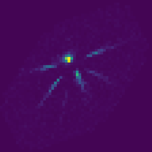
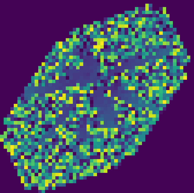
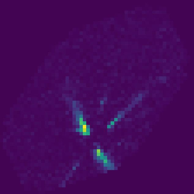
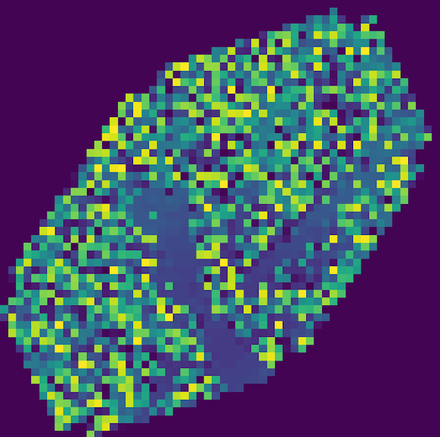
Figure 1: Example of a gamma and hadron events transformed to a square image. From left to right: gamma intensity, gamma timing, hadron intensity, hadron timing.

3.2 Energy Bands

The BDTs that we compared against operated on specific energy bands. This is a common approach meant to simplify models and speed up training time. We applied the same splitting of the data to train the CNNs. We tested 5 energy bands, as shown in table 1. Each energy band had approximately two times more signal than background events. Half the events were used for training, half for validation.

4 Network Architecture

Following the survey work from [20], we decided to start from the best network according to their study, namely InceptionV3 [21]. We did not explore the hyper-parameters space either and only used ADADELTA [22] for the optimizer and binary cross-entropy [23] for the loss function. We focused instead on the network architecture, and quickly found out that InceptionV3 has too many layers for the task at hand. This makes sense as InceptionV3 was designed to classify images into one thousand categories, while we only have two possible outputs (gamma / hadron).

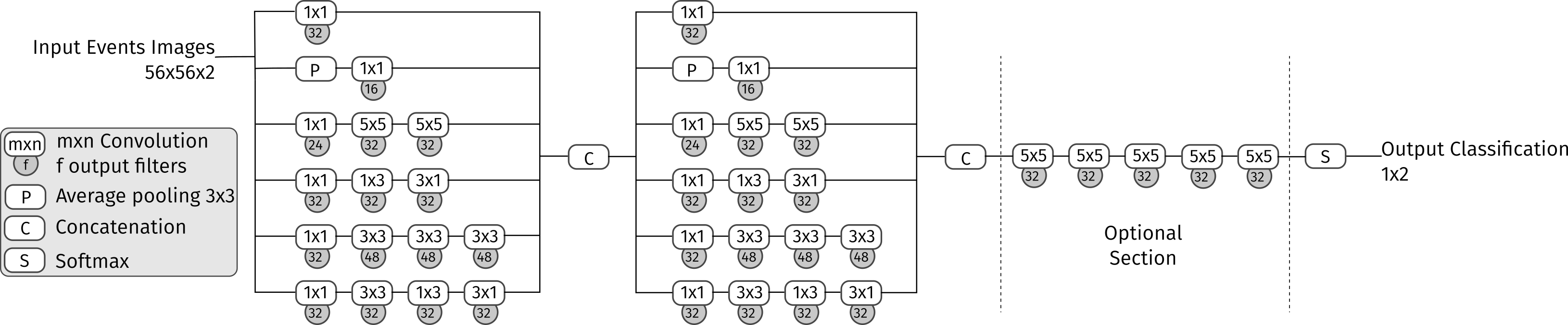
Figure 2: Overall architecture of the CNN used for this study. The optional section is only present for the model with 595k parameters.

After some trial-and-error we ended up with a baseline architecture that has nine layers for a total of 290k parameters (DL290k - figure 2). We also tested two variants of this architecture:

• Simplified: same as the baseline architecture, but with half the number of filters for each convolution kernel. Total parameters: 18k (DL18k)

• Extended: same as the baseline architecture, but with extra convolutions before the softmax layer [24]. Total parameters: 595k (DL595k)

There was no dropout layer [25] included in the model. The reason for this is two-fold. First, adding dropout layers significantly decreased the performance of the model and slightly increased the training time. Second, because we have virtually unlimited simulated data to train the models, overfitting can be dealt with by increasing the size of the training dataset.

5 Results

Even though results are presented in the form of ROC curves below, in reality the ratio of signal/background events is in the order of $\frac{1}{10000}$. It is thus very important that the ROC curve be as steep as possible so as to limit the contamination of the signal by background events. The CNNs peaked between epoch 7 and 59 depending on the training parameters before starting to overfit on the training data. They performed in a very similar way to the BDTs, as seen in table 1. This result is quite encouraging, as no a-priori knowledge was given to the CNNs. On the contrary a lot of human expertize was put in the training of the BDTs, even if the models that we compared against may not be the best possible ones. CNNs outperformed BDTs at high energies, while the opposite is true at low energies (figure 3, left). The differences are more obvious in the zoomed-in plots on figure 3, middle. In this plot, CNNs outperform BDTs in most cases, despite having higher AUCs. This discrepancy can be understood when looking at the other zoomed-in curves in figure 3, right.

Table 1: Summary of the performance (area under curve - AUC) of the different models for each energy band (EB) and for each model.

EB	Num. Evts	AUC BDT	AUC DL18k	AUC DL290k	AUC DL595k
63 to 158 GeV	354k	0.9759	0.9600	0.9648	0.9707
100 to 562 GeV	800k	0.9861	0.9807	0.9851	0.9869
316GeV to 1.8 TeV	400k	0.9904	0.9913	0.9923	0.9920
1 to 5.6 TeV	200k	0.9923	0.9950	0.9963	0.9947
3.1 to 32 TeV	120k	0.9934	0.9930	0.9958	0.9948

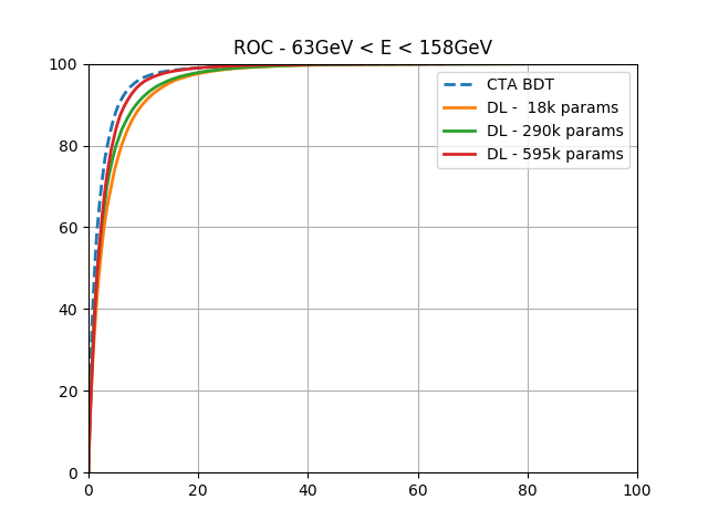
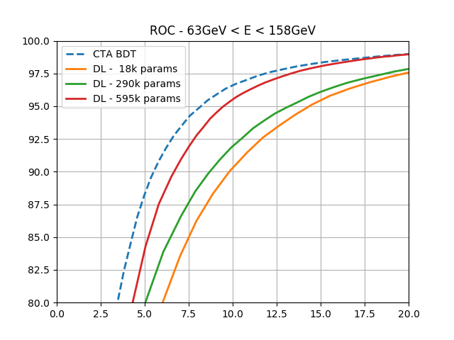
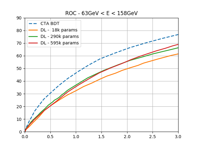
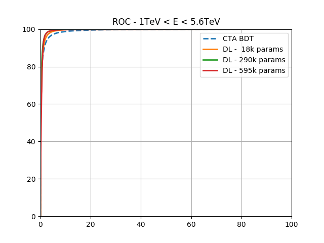
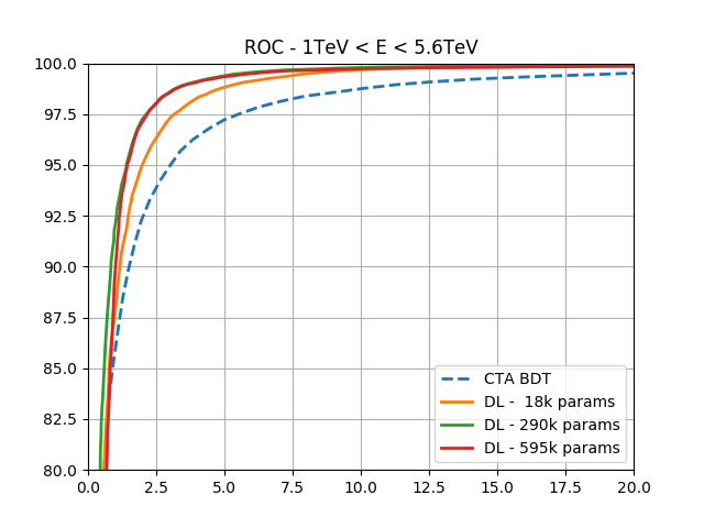
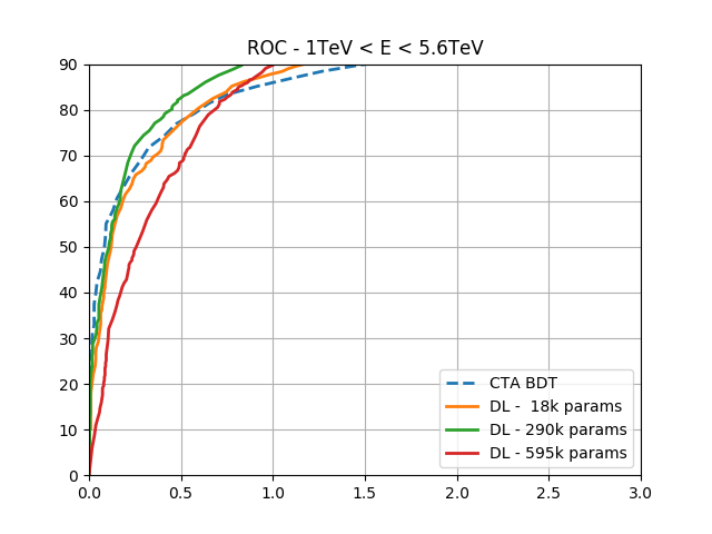
Figure 3: ROC curves for energy from 63 to 158GeV, for which BDTs outperformed CNNs, and from 1 to 5.6TeV, for which CNNs outperformed BDTs. Left: zoomed out view, middle: zoom in the central region, right: zoom in the beginning region

In this plot, it becomes clear that the ROC curve of the BDTs has a steeper start than CNNs, for all energy bands, which explains the higher overall AUC. Consequently, the best performing approach will depend on where one applies the cut to separate signal from background. Rejecting as much background as possible while possibly discarding some signal events would make the BDTs win, while accepting as many signal events along with more background would make the CNNs win. Figuring out the most optimal cut is always a trade-off between significance and sensitivity, and different cuts might be more adapted to specific science goals. We tackled the steepness of the ROC curves problem by training the CNNs with ten times more events. In this case it appeared that the overall accuracy does not improve but the slope of the beginning of the ROC curve became steeper, in-par with the BDTs. This hints that the current shortcomings of CNNs may be addressed simply by augmenting the training datasets with more events.

6 Conclusion

In this paper, we investigated a fair comparison between a state-of-the-art classification technique for Cherenkov telescopes data and convolutional neural networks. By applying standard CNN architectures and adapting the Cherenkov data to it, we demonstrated performances that are close to or already better than existing techniques. This suggest that research in CNNs and other novel machine learning approaches should be actively pursued to help achieve the best science output of the upcoming CTA observatory.
Many aspects of this investigation will be taken further as there seems to be much room for improvement. The datasets could be improved by keeping not only two values but rather the full waveforms. The neural network architecture could be improved by implementing hexagonal convolutions. The robustness of the results should be verified by continuing similar comparisons with other, extended datasets. Finally, the issue of having simulated data that is not identical to the real data should be addressed.

We would like to thank G Maier for kindly providing the list of Monte-Carlo events along with the output of the BDT analysis. L. Arrabito and J. Bregeon for helping us in our adventure to retrieve data from the GRID. The CADMOS (www.cadmos.org) for granting us the compute hours at CSCS that made this study possible. The CSCS staff for kindly handling our questions and problems. The CTA SAPO for kindly reviewing our paper internally. We gratefully acknowledge financial support from the agencies and organizations listed here: http://www.cta-observatory.org/consortium_acknowledgments

References

- [1] Shilon I et al. 2018 ArXiv e-prints (Preprint 1803.10698)
- [2] The Cherenkov Telescope Array Consortium 2017 ArXiv e-prints (Preprint 1709.07997)
- [3] Coadou Y 2013 European Physical Journal Web of Conferences vol 55
- [4] Maier G and Holder J 2017 Proceedings of the 35th International Cosmic Ray Conference (Preprint 1708.04048)
- [5] Breiman L 2001 Mach. Learn. 45 5–32 ISSN 0885-6125
- [6] de Naurois M and Rolland L 2009 Astroparticle Physics 32 231–252 (Preprint 0907.2610)
- [7] Hu J et al. 2017 CoRR abs/1709.01507 (Preprint 1709.01507)
- [8] Russakovsky O et al. 2015 International Journal of Computer Vision (IJCV) 115 211–252
- [9] Schawinski K et al. 2017 Monthly Notices of the Royal Astronomical Society: Letters 467 L110–L114
- [10] Hezaveh Y D et al. 2017 Nature 548 555–557 (Preprint 1708.08842)
- [11] Schaefer C et al. 2018 Astronomy and Astrophysics 611 A2 (Preprint 1705.07132)
- [12] Stark D et al. 2018 Monthly Notices of the Royal Astronomical Society 477 2513–2527 (Preprint 1803.08925)
- [13] Erdmann M et al. 2018 Astroparticle Physics 97 46–53 (Preprint 1708.00647)
- [14] The Pierre Auger Collaboration 2015 Nuclear Instruments and Methods in Physics Research 798 172 – 213 ISSN 0168-9002
- [15] George D and Huerta E A 2018 Physics Letters B 778 64–70 (Preprint 1711.03121)
- [16] The LIGO Scientific Collaboration 2012 Classical and Quantum Gravity 29 129602
- [17] Deng J et al. 2009 CVPR09
- [18] Park N 2015 34th International Cosmic Ray Conference (Preprint 1508.07070)
- [19] Moralejo A et al. 2009 31st International Cosmic Ray Conference, ICRC 2009
- [20] Castano D N et al. (CTA) 2018 PoS ICRC2017 809 (Preprint 1709.05889)
- [21] Szegedy C et al. 2016 IEEE Conference on Computer Vision and Pattern Recognition pp 2818–2826
- [22] Zeiler M D 2012 CoRR abs/1212.5701
- [23] Mannor S et al. 2005 Proceedings of the 22Nd International Conference on Machine Learning pp 561–568
- [24] Bishop C M 2006 Pattern Recognition and Machine Learning (Information Science and Statistics) (Berlin, Heidelberg: Springer-Verlag) ISBN 0387310738
- [25] Hinton G E et al. 2012 CoRR abs/1207.0580