High-dimensional temporal mode propagation in a turbulent environment

Abstract

Temporal modes of photonic quantum states provide a new framework to develop a robust free-space quantum key distribution (QKD) scheme in a maritime environment. We show that the high-dimensional temporal modes can be used to fulfill a persistent communication channel to achieve high photon-efficiency even in severe weather conditions. We identify the parameter regimes that allow for a high-fidelity quantum information transmission. We also examine how the turbulent environment affects fidelity and entanglement degree in various environmental settings.

I INTRODUCTION

The past decades have seen a great deal of interest in photonic quantum communication key-11-1 from several motivations including the security of the quantum key distribution (QKD) in the presence of environmental noise key-1 ; key-2 ; key-2-1 , the persistence of entanglement in terms of Bell inequality violation key-3 , quantum network key-4 , and the transfer between flying qubits (photons) and stationary qubits (atoms etc.) key-5 ; key-6 . From a more fundamental physics viewpoint, the free-space quantum communication offers a great potential of distributing information via photons promising, in principle, unconditional security key-7 ; key-8 ; key-9 ; key-10 . In practice, however, it has been shown in many realistic contexts for deployment that the errors caused by noises or imperfections remain the major obstacles in implementing a reliable long-distance quantum channel when the environmental factors are not taken into account properly key-2 ; key-11 ; key-12 .

Several prominent quantum communication protocols have been focused on exploring the aspects of photonic variables that allow efficient quantum state preparations, manipulations and detections key-1 ; key-3 ; key-15 ; key-16 ; key-17 ; key-18 ; key-19-1 ; key-20-1 ; key-1322 ; key-35 ; key-36 ; key-36-1 ; key-4333 ; key-73-1 ; key-19 . For example, the photon polarizations have been widely used in implementing quantum key distribution (QKD) scheme in many physical settings key-1 ; key-3 . However, apart from the well-known issues associated with the photon generation, detection efficiency, and polarization imperfections, it also becomes clear that the low-dimensional states formed by photon polarizations may be vulnerable to the effect of environmental noises. Hence, it may impose a limit on the capacity of the quantum communication channels. As such, recent research has extended to the high-dimensional spaces exploiting the advantages of multi-state systems generally called qudits. In this context, several other types of degrees of freedom of a single photon have been used to encode information including orbital angular momentum (OAM) key-15 ; key-16 ; key-17 ; key-18 ; key-19-1 ; key-20-1 , momentum-positionkey-1322 , temporal modes key-35 ; key-36 ; key-36-1 , and time-energy key-4333 ; key-73-1 ; key-19 , to name a few. While the qudit systems offer advantages in the photon information capacity with high levels of security, in practical implementations, there are still some shortcomings to be overcome such as the reliable OAM state generation and the perturbation sensitivity of scattering and absorption.

A maritime environment is notorious for causing various errors due to scattering, absorption, and turbulence. It is imperative that the focus of free-space quantum communication be broadened to examine the feasibility of implementing high-dimensional photon states, which are known to be sensitive to the atmospheric perturbation such as turbulence. In general, the vulnerability of the photons in different frequency domains to the turbulence destruction still remain under investigated. Most theoretical studies engaging photon free-space communication are usually conducted within the framework of weak scintillation, which cannot be completely reliable if the near-sea-level implementation of the QKD scheme is needed. Several approaches have been studied to overcome the reduction of implementation feasibility of photon communication channel for high-dimensional angular OAM states in a maritime environment, a focus on a systematic investigation on the temporal photonic mode propagation in a turbulent scenario is clearly desirable.

In this paper, we will consider free-space temporal mode propagation encoded by either a single photon or an entangled photon pair through a maritime environment. Our purpose is to examine the robustness and practicality of implementing a QKD channel in the presence of maritime noise sources such as scattering, absorption and turbulence. In particular, we will employ the so-called infinitesimal propagation method to simulate the temporal mode propagation in the atmospheric setting with varied turbulence strengths . We show by numerical simulations that the temporal modes as the information carriers can be used to efficiently generate quantum keys in certain frequency ranges even in the strong presence of turbulence. We also identify some frequency ranges to be not an ideal choice for implementing a near-sea surface quantum channel due to the scattering and absorption processes when a near-sea surface implementation is needed.

The structure of the paper is organized as follows. First, in Sec. II, we make a brief summary of our numerical simulations on the feasibility of the frequency ranges in the optical communication in a maritime environment when the scattering and absorption processes are taken into account. Such a general survey is useful in putting our investigation into perspective, and may be used to identify the frequency ranges that will underpin the persistent photonic communication in a maritime environment. In Sec. III, we study the feasibility of the temporal mode implementations under the influence of turbulence. We conclude in Sec. IV., while some technical details are left in Appendix A.

II Photonic communication in a generic maritime environment

To begin, we first investigate through numerical simulations how a maritime environment affects the photon propagation in various parameter regimes. For a free-space optical communication system, there are many atmospheric factors that can significantly impact photon propagation including scattering, absorption and turbulence. The previous work on studying the free-space optical communication channels has shown that the environmental noises may affect the photon propagation at every stage of the process, from the generation of photons, propagation, to ultimately their detection by receivers. In particular, in the propagation process, the loss of photons due to scattering or absorption may reduce the efficacy of communication to such a level to make a reliable communication impossible. Therefore, the successful implementation of a theoretical concept of optical communication protocol requires a deeper understanding of how the photon beams with different wavelengths interacting with an atmospheric environment.

Such an investigative survey through numerical simulations of pulsed photon beam propagation in the maritime atmosphere will provide an useful picture about the environment-system interaction as a whole, and will be the first step for pinpointing some optimal parameter regimes that underpin reliable high efficiency free-space communication. For this purpose, we have tested and conducted a Monte-Carlo method to study the generic influence of atmospheric aerosols on the photon communication in a maritime setting. For the processes involving molecule scattering and absorption, we have used the 1976 U.S. Standard atmospheric model key-22-1 . Moreover, we have employed Mie scattering theory in our analysis key-27 ; key-28 and we have extensively used the aerosol parameters from the Advanced Navy Aerosol Model (ANAM) key-25-1 ; key-26 .

Without loss of generality, we assume that the heights of the transmitter and receiver are both at $19\ \text{m}$ for a $30\ \text{km}$ propagation range, the photon beams emitted at this height have at least $1.36\ \text{m}$ clearance from the ocean surface, therefore, the photon beams are, by and large, well above the ocean waves in their propagation processes. Since the environmental impacts caused by atmospheric extinction between the transmitter and receiver may have very large variations, it is desirable to describe the dynamical processes beyond a naive statistical average approach. Moreover, in order to make our numerical simulations more dependable for the implementation of real-world quantum communication protocols, we have considered a wide parameter range including high relativity humidity, large air mass parameters and large wind speeds to reflect the severe weather conditions. The major findings based on our numerical simulations are summarized in Fig. (1), which exhibits a paradigmatic case involving a Gaussian beam with $10\ \text{km}$ Rayleigh range, and the assumption that the receiver is placed at $z_{f}=30\ \text{km}$. Among many informative results, the simulations have indicated that the wavelength at $3.95\ \text{$\mu$m}$ is a desirable choice for the implementation of maritime optical communication. The numerical survey has paved the way for further investigations of the QKD implementation in a maritime environment. It should be emphasized, excluding some wavelengths that are known to prone to the water absorption, that there exist other wavelength ranges (e.g., $9-10\ \mu m$) that might be equally feasible for the maritime QKD realization. However, the lack of a reliable long-wave length single photon source and the detection inefficiency are hindering their applications. Throughout our numerical simulations, we have selected $\frac{\omega_{p}}{2}=\frac{2\pi c}{\lambda}\approx 477\ \text{THz}$ as our center frequency.

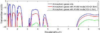
Figure 1: Near center transmittance of Gaussian beams with 10km Rayleigh length. Red: air mass parameter $p=6$, wind speed $w=10\ \text{m/s}$, height $h=20\ \text{m}$, relative humidity $s=0.8$. Green: air mass parameter $p=10$, wind speed $w=10\ \text{m/s}$, height $h=19\ \text{m}$, relative humidity $s=0.95$.

III Photon propagation in a turbulence environment

III.1 Schmidt decomposition of bi-photon states

For implementing a quantum communication protocol, let us now consider, at the transmitter part, a two-photon state, generated by a nonlinear crystal, represented by a Schmidt decomposition. This situation under consideration is to assume that the down-converted beams are constrained to be collinear with the pump beams through the use of pinholes. More explicitly, a double-Gaussian spectral state may be written as key-19 ,

$$|\Psi\rangle =\sqrt{\frac{2}{\pi\sigma_{a}\sigma_{b}}}\int d\omega_{1}\int d\omega_{2}\exp\left[-\frac{(\omega_{1}+\omega_{2}-\omega_{P})^{2}}{2\sigma_{a}^{2}}\right]$$

$$\quad\cdot\exp\left[-\frac{(\omega_{1}-\omega_{2})^{2}}{2\sigma_{b}^{2}}\right]|\omega_{1}\rangle|\omega_{2}\rangle$$ (1)

where $\sigma_{a}$ is determined by the coherence time of the pump field, and $\sigma_{b}$ is determined by the phase matching bandwidth of the spontaneous parametric down-conversion (SPDC) source key-20 . For a typical SPDC source, the range of $\sigma_{b}$ is on the order of hundreds of MHz to several hundreds THz. Here, for our applications, the spatial mode of each frequency can be treated as a Laguerre-Gaussian mode with the lowest radial and azimuthal indices (known as Gaussian beams) key-21 .

For the above double-Gaussian state, an analytical expression for the Schmidt decomposition is known as key-22 ; key-23 ,

$$|\Psi\rangle =\sum_{n=0}^{\infty}\sqrt{\lambda_{n}}|f_{n}\rangle|f_{n}\rangle\text{,}$$ (2)

with the eigenvalues $\lambda_{n}$ and the corresponding eigenstates $|f_{n}\rangle$,

$$\lambda_{n} =\frac{4\sigma_{a}\sigma_{b}(\sigma_{a}-\sigma_{b})^{2n}}{(\sigma_{a}+\sigma_{b})^{2(n+1)}},$$ (3)

$$|f_{n}\rangle \equiv\int d\omega f_{n}(\omega)|\omega\rangle$$ (4)

$$=\int d\omega\left(\frac{2}{\sigma_{a}\sigma_{b}}\right)^{\frac{1}{4}}\left(2^{n}n!\sqrt{\pi}\right)^{-\frac{1}{2}}\exp\left[-\frac{(\omega-\frac{\omega_{P}}{2})^{2}}{\sigma_{a}\sigma_{b}}\right]$$

$$\quad\cdot H_{n}\left(\sqrt{\frac{2}{\sigma_{a}\sigma_{b}}}(\omega-\frac{\omega_{P}}{2})\right)|\omega\rangle,$$ (5)

where $H_{n}(x)$ is the $n$th Hermite polynomial of $x$. Note that $\lambda_{n}\rightarrow 0$ very quickly for a large $n$. Setting $b=\frac{2}{\sigma_{a}\sigma_{b}}$ and $\tilde{\omega}=\omega-\frac{\omega_{p}}{2}$, as an illustration, the first four modes are given by,

$$|f_{0}\rangle =\int d\omega\left(\frac{b}{\pi}\right)^{\frac{1}{4}}e^{-\frac{b}{2}\tilde{\omega}^{2}}|\omega\rangle,$$ (6)

$$|f_{1}\rangle =\int d\omega\left(\frac{4b^{3}}{\pi}\right)^{\frac{1}{4}}e^{-\frac{b}{2}\tilde{\omega}^{2}}\tilde{\omega}|\omega\rangle,$$ (7)

$$|f_{2}\rangle =\int d\omega\left(\frac{b}{64\pi}\right)^{\frac{1}{4}}e^{-\frac{b}{2}\tilde{\omega}^{2}}(4b\tilde{\omega}^{2}-2)|\omega\rangle,$$ (8)

$$|f_{3}\rangle =\int d\omega\left(\frac{b^{3}}{768\pi}\right)^{\frac{1}{4}}e^{-\frac{b}{2}\tilde{\omega}^{2}}(8b\tilde{\omega}^{3}-12\tilde{\omega})|\omega\rangle.$$ (9)

Note that the higher orders can also be obtained in a straightforward way. As it becomes clearer later, the higher-order modes give negligible contributions to our analysis. Fig. 2 plots the basic behaviors of these four functions.

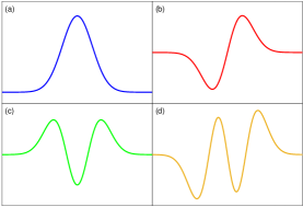
Figure 2: First four Schmidt mode coefficients. Blue: $f_{0}$. Red: $f_{1}$. Green: $f_{2}$. Yellow: $f_{3}$.

The Schmidt number that characterizes the degree of photonic entanglement in the state $|\Psi\rangle$ is given by

$$K =\left(\sum_{n=0}^{\infty}\lambda_{n}^{2}\right)^{-1}=\frac{\sigma_{a}^{2}+\sigma_{b}^{2}}{2\sigma_{a}\sigma_{b}}.$$ (10)

In our analysis, the condition $\sigma_{a}\ll\sigma_{b}$ is generally valid, thus the Schmidt number can be approximated as

$$K \approx\frac{\sigma_{b}}{2\sigma_{a}}.$$ (11)

Clearly, the parameter $\sigma_{a}$ of the pump laser is directly related to the number of modes giving rise to a significant contribution to the Schmidt number.

By using the mode-selective detection on photon 1, we can collapse photon 2 (transmitting photon) onto one of the Schmidt modes. For a high dimensional photonic state, the information is encoded into the mode numbers. To be more specific, in the following discussions, we may set $\sigma_{a}=10\ \text{THz}$ and $\sigma_{b}=80\ \text{THz}$. For our purpose, we only consider the first four modes for encoding the information to be transmitted through a noisy channel. It can be easily shown that the probability $\lambda_{n}$ of finding the state to be projected to those first four modes is given by $0.395$, $0.239$, $0.145$, and $0.087$ respectively. As such, we see that only $13.4\%$ of modes are discarded in state generation step. The normalized output state from SPDC is

$$|\Psi\rangle \approx(1.15)\sum_{n=0}^{3}\sqrt{\lambda_{n}}|f_{n}\rangle|f_{n}\rangle,$$ (12)

Throughout this paper, in order to avoid the degeneracy, we always prepare the initial state in the same transverse profile (Gaussian beam),

$$|f_{n}\rangle =\int d\omega f_{n}(\omega)|0_{\omega}\rangle$$ (13)

In the next subsection, we consider how an initial photonic state evolves in a noisy environment.

III.2 Infinitesimal propagation equation

An infinitesimal propagation equation (IPE) method for a single photon with a fixed wavelength passing through a turbulent media has been studied before in the seminal work key-29 ; key-30 ; key-31 . Under the monochromatic approximation, an arbitrary pure state of a single photon can be expressed as (assuming the polarization is uniform and may be ignored)

$$|\psi\rangle =\int G(\mathbf{K},z)|\mathbf{K}\rangle\frac{d^{2}K}{4\pi^{2}}.$$ (14)

We use $z$ to denote the propagation direction where $\{|\mathbf{K}\rangle\}$ is the two-dimensional momentum basis of the transverse plane, and $G(\mathbf{K},z)$ is the two-dimensional momentum space wave function. The inverse Fourier transform of $G(\mathbf{K})$ gives the position space wave function $g(x,y)$ in the transverse plane.

The equation of motion of the space wave function in the media can be written as

$$\nabla^{2}E(\mathbf{x})+k^{2}n^{2}(\mathbf{x})E(\mathbf{x}) =0,$$ (15)

where $\mathbf{x}$ is the three dimensional position vector, $E(\mathbf{x})$ is the scalar part of the electric field, $k=\frac{\omega}{c}$ is the wave number and $n(\mathbf{x})$ is the index of refraction. In general, $n$($\mathbf{x}$) is also a function of $k$. Since the differences of $n(\mathbf{x})$ in a narrow frequency range are negligible, we may treat the refractive index as a frequency-independent quantity.

The refractive index $n(\mathbf{x})$ in a turbulent atmosphere may be split into two parts,

$$n(\mathbf{x}) =1+\delta n(\mathbf{x}).$$ (16)

The second term $\delta n(\mathbf{x})$ is spatially dependable, and it is typically small compared to the first term (which is one). Thus, an approximate Helmholtz equation may be obtained from Eq. (15),

$$\nabla^{2}E(\mathbf{x})+k^{2}E(\mathbf{x})+2k^{2}\delta n(\mathbf{x})E(\mathbf{x}) =0.$$ (17)

Here, we have assumed that the beam is paraxial and propagates in the z-direction. If we decompose $E(\mathbf{x})\equiv g(\mathbf{x})e^{-ikz}$, we can get the following paraxial wave equation for $g(\mathbf{x})$,

$$\nabla_{T}^{2}g(\mathbf{x})-2ik\partial_{z}g(\mathbf{x})+2k^{2}\delta n(\mathbf{x})E(\mathbf{x}) =0.$$ (18)

Using the inverse two-dimensional Fourier transform

$$g(\mathbf{x}) =\int G(\mathbf{K},z)e^{-i\mathbf{K}\cdot(x,y)}\frac{d^{2}K}{4\pi^{2}},$$ (19)

we obtain

$$\partial_{z}G(\mathbf{K},z) =\frac{i}{2k}|\mathbf{K}|^{2}G(\mathbf{K},z)-ikN(\mathbf{K},z)\star G(\mathbf{K},z)$$ (20)

where $N(\mathbf{K},z)$ is the inverse two-dimensional Fourier transform of $\delta(\mathbf{x})$ and $\star$ stands for the convolution product.

The density operator for a fixed wavelength single photon state can be expressed in the orbital angular momentum (OAM) basis,

$$\rho =\sum_{m,n}\rho_{m,n}|m\rangle\langle n|.$$ (21)

where $m,n$ are collective indices for both the radial ($r$) and orbital degrees ($l$) of the Laguerre-Gaussian (LG) modes ($m=\{r_{m},l_{m}\}$) and $|m\rangle=\int G_{m}(\mathbf{K},z)\frac{d^{2}K}{4\pi^{2}}$.

From key-29 ; key-30 ; key-31 , we get

$$\partial_{z}\rho_{u,v}(z) =S_{m,u}(z)\rho_{m,v}-S_{v,n}(z)\rho_{u,n}$$

$$\quad+L_{m,n,u,v}(z)\rho_{m,n}-L_{T}\rho_{m,n}.$$ (22)

The first two non-dissipative terms in the above equation describe the free-space propagation, whereas the last two dissipative terms delineate how the turbulence causes the transition among the LG modes through scattering processes. The operator that represents the free-space propagation without loss is given by,

$$S_{p,q}(z) =\frac{i}{2k}\int|\mathbf{K}|^{2}G_{x}(\mathbf{K},z)G_{y}^{*}(\mathbf{K},z)\frac{d^{2}K}{4\pi^{2}}.$$ (23)

More explicitly, the dissipative terms of the evolution are given by

$$L_{T} =k^{2}\int\Phi_{1}(\mathbf{K})\frac{d^{2}k}{4\pi^{2}},$$ (24)

$$L_{m,n,u,v}(z) =k^{2}\int\Phi_{1}(\mathbf{K})W_{m,u}(\mathbf{K},z)W_{n,v}^{*}(\mathbf{K},z)\frac{d^{2}K}{4\pi^{2}},$$ (25)

with

$$W_{p,q}(\mathbf{K},z) =\int G_{p}(\mathbf{K}_{1},z)G_{q}^{*}(\mathbf{K}_{1}-\mathbf{K},z)\frac{d^{2}K_{1}}{4\pi^{2}}.$$ (26)

It should be noted, in the above equations, that the propagation vector $\mathbf{K}=(k_{x},k_{y})$ represents the two-dimensional projection of the three-dimensional propagation vector $\mathbf{k}=(k_{x},k_{y},k_{z})$ and the function $G_{p}(\mathbf{K},z)$ is the two-dimensional momentum space wave function.

The formalism presented here is valid for an arbitrary power spectral density. In Kolmogorov turbulence theory [citation] if we ignore the effect of the inner scales and use the von Karman power spectral density, the refractive index power spectral density $\Phi_{1}(\mathbf{K})$ can be written as,

$$\Phi_{1}(\mathbf{K}) =\frac{0.033(2\pi)^{3}C_{n}^{2}(z)}{(|\mathbf{\mathbf{K}}|^{2}+\kappa_{0}^{2})^{\frac{11}{6}}},$$ (27)

where $\kappa_{0}$ is the lager outer scale parameter and $C_{n}^{2}(z)$ is the refractive index structure constant at point $z$.

Substituting Eq. (27) into Eq. (24), we get

$$L_{T} =(30.86)C_{n}^{2}\lambda^{2}\kappa_{0}^{-\frac{5}{3}},$$ (28)

$$L_{m,n,u,v}(z) =\sum_{j_{1},j_{2}=0}^{\infty}\delta_{mu}\delta_{n\nu}L_{T}+8.1\delta_{l_{m}-l_{u},l_{n}-l_{v}}l(z)$$

$$\quad\cdot 2^{j_{1}+j_{2}}\Gamma\left[\frac{j_{1}+j_{2}}{2}-\frac{5}{6}\right]c_{m,u,j_{1}}c_{m,u,j_{2}}^{*},$$ (29)

with

$$l(z) =C_{n}^{2}(z)\lambda^{-2}w_{0}^{\frac{5}{3}}\left(1+(\frac{\lambda z}{\pi w_{0}^{2}})^{2}\right)^{\frac{5}{6}}$$ (30)

$$\propto\begin{cases}w_{0}^{\frac{5}{3}}\lambda^{-2}&z\ll z_{R}=\frac{\pi w_{0}^{2}}{\lambda}\\ w_{0}^{-\frac{5}{3}}\lambda^{-\frac{1}{3}}&z\gg z_{R}=\frac{\pi w_{0}^{2}}{\lambda}\end{cases}.$$ (31)

where the relation $\lambda=\frac{2\pi}{k}$ is used. $c_{m,u,j_{1}}$ are the coefficients (for explicit expressions, see Appendix A). It is easy to check that $L_{T}$ diverges for large outer scales ($\kappa_{0}\rightarrow 0$). Note that $L_{m,n,u,v}(z)$ contains a counter term to cancel $L_{T}$. Besides, the non-zero terms of $L_{m,n,u,v}(z)$ exist only when $l_{m}-l_{u}-l_{n}+l_{v}=0$.

In key-29 ; key-30 ; key-31 , Roux has shown that the integral in Eq. (23) is non-zero only if the azimuthal indices are equal and the radial indices differ at most by one,

$$S_{m,n}(z) =\begin{cases}\frac{i(1+|l|+2r)}{2z_{R}}&\begin{cases}l_{m}=l_{n}=l\\ r_{m}=r_{n}=r\end{cases}\\ \frac{i(1+|l|+r)^{\frac{1}{2}}(1+r)^{\frac{1}{2}}}{z_{R}}&\begin{cases}l_{m}=l_{n}=l\\ |r_{m}-r_{n}|=1\\ r=min\{r_{m},r_{n}\}\end{cases}\\ 0&{\rm otherwise},\end{cases}$$ (32)

where $z_{R}$ is the Rayleigh range of the LG modes. $r_{m}$ and $l_{m}$ are the radial and orbital degrees of $m$th LG mode, respectively.

From Eq. (22) we can see that high order modes will be involved even if the initial state only contains one lowest mode (Gaussian beam) and $\delta n(\mathbf{\text{x}})=0$ (without scintillation). The reason is that Roux treated $\partial_{z}\rho_{u,v}(z)=\text{Tr}[(\partial_{z}\rho(z))|u\rangle\langle v|]$ for transverse planes around $z=z_{0}$ and kept $|m\rangle=\int G_{m}(\mathbf{K},z_{0})\frac{d^{2}K}{4\pi^{2}}$ unchanged. In order to simplify the process, we treat $\partial_{z}\rho_{u,v}(z)=\partial_{z}\text{Tr}[\rho(z)|u\rangle\langle v|]$ and keep $z$-dependent basis, the first terms in Eq. (22) vanish. New IPE can be written as

$$\partial_{z}\rho_{u,v}(z) =L_{m,n,u,v}\rho_{m,n}-L_{T}\rho_{m,n}.$$ (33)

If we reorganize the density matrix $\rho$ into a column vector $\rho^{r}$ by transposing every rows and merging them one by one, we can have

$$\partial_{z}\rho^{r} =R\rho^{r}.$$ (34)

The elements of the new matrix $R$ is obtained by $L_{m,n,u,v}$ and $L_{T}$.

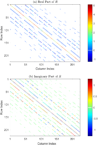
Figure 3: Example of the operator $R$ when $z=z_{R}$. All azimuthal indices go from $-2$ to $2$ and all radical indices go from $0$ to $2$. Here we set $L_{0,0,0,0}-L_{T}=1$. (Jet colormap)

In general, Eq. (33) represents a set of coupled first-order differential equations. The couplings allow transitions between two different modes. So even when the initial state contains only a few lower order modes, the turbulence will couple those lower order modes to all the other modes. Truncating this set of coupled equations, one may get rid of some couplings among the participating modes. Moreover, our numerical results have shown that the transitions become important when the following conditions hold,

$$\begin{cases}l_{m}-l_{u}=l_{n}-l_{v}=0,\ |r_{m}-r_{u}|=|r_{n}-r_{v}|=0\\ l_{m}-l_{u}=l_{n}-l_{v}=0,\ |r_{m}-r_{u}|+|r_{n}-r_{v}|=1\\ l_{m}-l_{u}=l_{n}-l_{v}=\pm 1,\ |r_{m}-r_{u}|=|r_{n}-r_{v}|=0\\ l_{m}-l_{u}=l_{n}-l_{v}=\pm 1,\ |r_{m}-r_{u}|+|r_{n}-r_{v}|=1,\ 2\end{cases}$$ (35)

In particular, the first three cases give the most contributions. It is interesting to know that when the azimuthal indices are unchanged, we can barely see both $|r_{m}-r_{u}|$ and $|r_{n}-r_{v}|$ to be equal to one. In Fig. (3), we find that, for the OAM modes the transitions mostly occur among their neighboring modes, and the transition between high order and lower order modes are practically impossible. Thus, the truncation used in IPE will contain enough useful information about the propagation. Now we use a different Lindblad form of IPE, written as

$$\partial_{z}\rho_{u,v}(z) =L_{m,n,u,v}\rho_{m,n}-\frac{1}{2}L_{n,n,m,u}\rho_{m,v}$$

$$\quad-\frac{1}{2}L_{m,m,v,n}\rho_{u,n}.$$ (36)

Eq. (33) and Eq. (36) are exactly equal since $\sum_{n}L_{n,n,m,u}=\delta_{m,u}L_{T},\ \sum_{m}L_{m,m,v,n}=\delta_{v,n}L_{T}$. In Fig. (4), we plot the transition probabilities for the two different cut-off approximations. It can be seen that the two methods converge with increasing cut-off orders, indicating that both methods are consistent in giving good approximate solutions. More specifically, we set the cut off at $N=4$ for Eq. (33).

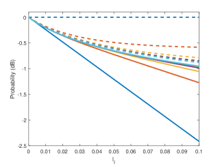
Figure 4: Example of a Gaussian beam with a wavelength $\lambda=3.95\ \text{$\mu$m}$ and Rayleigh length $z_{R}=10\ \text{km}$ propagating in a turbulent medium. $Y$ axis means the probability of finding the fundamental Gaussian mode while $l_{I}=\int_{0}^{z_{f}}d_{z}\ l(z)$ is a combination of multi parameters, including refractive index structure constant, distance, wavelength (waist size can be calculated). All azimuthal indices go from $-N$ to $N$ and all radical indices go from $0$ to $N$. For solid lines, we adapt the cut-off of Eq. (33), where $N$ goes from $0$ to $5$ from the bottom to the top; For dash lines, we use the cut-off of Eq. (36), where $N$ goes from $0$ to $5$ from the top to the bottom.

The density operator of an general spectro-temporal single photon in the OAM basis can be expressed as,

$$\rho =\int\int d\omega_{1}d\omega_{2}\Sigma_{m_{\omega_{1}},n_{\omega_{2}}}\rho_{m_{\omega_{1}},n_{\omega_{2}}}|m_{\omega_{1}}\rangle\langle n_{\omega_{2}}|,$$ (37)

where $m_{\omega_{j}},u_{\omega_{j}}$ are collective indices for both the radial and orbital degrees of Laguerre-Gaussian (LG) modes with frequency $\omega_{j}$($k_{j}$). Then the equation of motion is given by,

$$\partial_{z}\rho_{u_{\omega_{1}},v_{\omega_{2}}}(z) =L_{m_{\omega_{1}},n_{\omega_{2}},u_{\omega_{1}},v_{\omega_{2}}}(z)\rho_{m_{\omega_{1}},n_{\omega_{2}}}$$

$$\quad-(L_{T})_{\omega_{1},\omega_{2}}\rho_{u_{\omega_{1}},v_{\omega_{2}}},$$ (38)

with

$$(L_{T})_{\omega_{1},\omega_{2}} =k_{1}k_{2}\int\Phi_{1}(\mathbf{K})\frac{d^{2}K}{4\pi^{2}},$$ (39)

$$L_{m_{\omega_{1}},n_{\omega_{2}},u_{\omega_{1}},v_{\omega_{2}}}(z) =k_{1}k_{2}\int\Phi_{1}(\mathbf{K})W_{m_{\omega_{1}},u_{\omega_{1}}}(\mathbf{K},z)$$

$$\quad\cdot W_{n_{\omega_{2}},v_{\omega_{2}}}^{*}(\mathbf{K},z)\frac{d^{2}K}{4\pi^{2}}.$$ (40)

We note that more general cases can be dealt with similarly the above results after some necessary modifications.

III.3 Gaussian beam propagation in turbulence

We will assume that the initial state is a Gaussian beam $|0_{\omega}\rangle$ ($r=0,l=0$, lowest LG mode) with a fixed wavelength $\omega$. When the high order modes are ignored in the propagation process, the equation of motion is given by,

$$\partial_{z}\rho_{u,v}(z)= \sum_{m,n,u,v=0}^{3}L_{m,n,u,v}\rho_{m,n}-\sum_{m,n=0}^{3}L_{T}\rho_{m,n}.$$ (41)

In the limit of small $\kappa_{0}$, one finds that the most essential term is given by

$$L_{0,0,0,0}(z) \approx L_{T}-(54.11)l(z)$$ (42)

We define a probability of finding a photon in the lowest LG mode at position $z$ as

$$P(z) =\rho_{0,0}(z).$$ (43)

Having established the equation of motion (41), it is easy to show that the truncated density matrix gives rise to a pure decay for weak turbulence or short distances, and the probability in this regime is given by,

$$P(z) =e^{-(54.11)\int_{0}^{z}l(z^{\prime})dz^{\prime}}$$ (44)

Note that the strength of the scintillation is determined by $C_{n}^{2}$ with values ranging from $10^{-13}\ \text{m}^{-2/3}$ for strong turbulence to $10^{-17}\ \text{m}^{-2/3}$ for weak turbulence. To begin with, we first assume that the refractive index structure constant $C_{n}^{2}$ does not vary along the propagation path $z$. Then, from the analytical expression of $l(z)$, one can show that, for a given waist size, the average probability monotonically increases when the wavelength $\lambda$ increases. This observation is always valid independent of the propagation distance. For a fixed wavelength and propagation distance, we have shown that the minimum value of $l(z)$ occurs when $w_{0}=(\frac{\lambda z}{\pi})^{\frac{1}{2}}$ and numerical simulations show that the maximum value of probability $P$ occurs at around the value $w_{0}=\frac{3}{4}(\frac{\lambda z}{\pi})^{\frac{1}{2}}$ (see Fig.  (5)). It should be noticed that it is important to understand these dynamic behaviors when we consider the superposition of Schmidt modes, rather than one single transition mode.

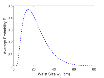
Figure 5: Average probability $P$ at receive plane. Distance z=30 km, wavelength $\lambda=3.95\ \text{$\mu$m}$, and the refractive index structure constant $C_{n}^{2}=10^{-16}\ \text{m}^{-2/3}$. The peak occurs at around $w_{0}=\frac{3}{4}(\frac{\lambda z}{\pi})^{1/2}\approx 14.57\ \text{cm}$.

When the propagation distance is significantly shorter than the Rayleigh range, the probability (43) may be further approximated by,

$$P \approx e^{-(3.25)\left(\frac{w_{0}}{r_{0}}\right)^{\frac{5}{3}}},$$ (45)

where so-called Fried parameter $r_{0}=0.185\left(\frac{\lambda^{2}}{C_{n}^{2}z}\right)^{\frac{3}{5}}$.

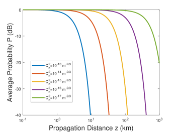
Figure 6: Average probability P of receiving the lowest LG mode versus propagation distance. Wavelength $\lambda=3.95\ \text{$\mu$m}$,waist size $w_{0}=\frac{3}{4}(\frac{\lambda z}{\pi})^{1/2}$. From left to right $C_{n}^{2}=\{10^{-13},10^{-14},10^{-15},10^{-16},10^{-17}\}\ \text{m}^{-2/3}$.

The average probability $P$ of finding photons at the position $z$ is shown to be an exponentially decaying function of the refractive index structure constant $C_{n}^{2}$. Therefore, it is difficult to realize the long range communication in the strong scintillation regime (see Fig.  (6)).

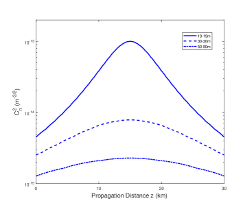
Figure 7: Refractive Index Structure Constants along the propagation path in an extreme bad weather condition. Sea level temperature $T_{sea}=15\textdegree C$, air temperature $T_{air}=20\textdegree C$, wind speed $w=5m/s$, and relative humidity $RH=98\%$. Solid line: $19-19\ \text{m}$; dash line: $30-30\ \text{m}$; dash-dot line: $50-50\ \text{m}$. Earth curvature is considered.

In general, $C_{n}^{2}(z)$ is highly sensitive to the propagation path height, but is relatively insensitive to the wavelength. Our simulations for the turbulence are based on varieties of parameter ranges to better reflect a real maritime environment.

It can be shown that when the wavelength is greater than $2\ \text{$\mu$m}$, the refractive index structure constant is no longer dependent on the wavelength key-32 ; key-33 . Our simulations investigate the bad weather condition represented by high relative humidity, strong wind speed and large air-sea surface temperature difference. Turbulence typically falls off sharply in the first few meters above the sea surface, then it varies slowly with the increasing height. To have a more accurate description of the long distance maritime communication, the Earth curvature should be taken into account. In Fig. (7), we have plotted three cases about the propagation path: the heights of the emitter and receiver are $19-19\ \text{m}$, $30-30\ \text{m}$, and $50-50\ \text{m}$, respectively. The results show that the strong turbulence may be avoided when the emitter and receiver are well above the sea surface. For example, in the $19-19\ \text{m}$ case, we see that the maximum refractive index structure constant along the propagation path $C_{n}^{2}$ is about $2\times 10^{-13}\ \text{m}^{-2/3}$, which makes practical communication impossible. Therefore, one needs to use other paths.

III.4 Temporal mode propagation

For an initial state prepared in the $n$th temporal mode, the reduced density operator can be written as

$$\rho_{n}^{i} =\int\int d\omega_{1}d\omega_{2}f_{n}(\omega_{1})f_{n}(\omega_{2})|0_{\omega_{1}}\rangle\langle 0_{\omega_{2}}|,$$ (46)

Since the infinitesimal propagation method also works for the cross terms $|0_{\omega_{1}}\rangle\langle 0_{\omega_{2}}|$($\lambda_{j}=\frac{2\pi c}{\omega_{j}}$), we find that the modified $l(\omega_{1},\omega_{2},z)$ takes the following form

$$l(\omega_{1},\omega_{2},z) \approx C_{n}^{2}(z)(\lambda_{1}\lambda_{2}){}^{-1}w_{0}^{\frac{5}{3}}$$

$$\quad\cdot\left[1+\frac{1}{2}(\frac{\lambda_{1}z}{\pi w_{0}^{2}})^{2}+\frac{1}{2}(\frac{\lambda_{2}z}{\pi w_{0}^{2}})^{2}\right]^{\frac{5}{6}}.$$ (47)

The influence of scintillation will typically evolve the initial pure state into a mixed state. For our purpose here, we only need to consider the lowest LG mode at the receive plane. Therefore, the truncated final density matrix at the propagation distance $z$ may be written as,

$$\rho_{n}^{f} =\int\int P(\omega_{1},\omega_{2})f_{n}(\omega_{1})f_{n}(\omega_{2})|0_{\omega_{1}}\rangle\langle 0_{\omega_{2}}|d\omega_{1}d\omega_{2}.$$ (48)

Figure 8: Average probability $P$ for both diagonal and cross terms. Propagation distance $z=30\ \text{km}$, waist size $w_{0}=14.57\ \text{cm}$ and the refractive index structure constant $C_{n}^{2}=10^{-16}\ \text{m}^{-2\text{/3}}$.

Note the trace of the density matrix (48) denoted by $T_{n}=\int P(\omega,\omega)|f_{n}(\omega)|^{2}d\omega$ is not 1. The decaying function $T_{n}$ represents the information of the transition from the $n$th mode to the other modes. The normalized density matrix $\rho_{n}^{N}$ is obtained by dividing $T_{n}$,

$$\rho_{n}^{N} =\frac{1}{T_{n}}\int\int P(\omega_{1},\omega_{2})f_{n}(\omega_{1})f_{n}(\omega_{2})|\omega_{1}\rangle\langle\omega_{2}|d\omega_{1}d\omega_{2}.$$ (49)

One can show that the probability of finding the photon at the receiver position in the $m$th mode is

$$S_{n,m} =\frac{1}{T_{n}}\int\int P(\omega_{1},\omega_{2})f_{m}(\omega_{1})f_{m}(\omega_{2})$$

$$\quad\cdot f_{n}(\omega_{1})f_{n}(\omega_{2})|\omega_{1}\rangle\langle\omega_{2}|d\omega_{1}d\omega_{2}.$$ (50)

We have set the distance z=30 km, wavelength $\lambda=3.95\ \text{$\mu$m}$, and the refractive index structure constant $C_{n}^{2}=10^{-15}\ \text{m}^{-2/3}$ to test our approach. The total traces (probabilities of finding this mode) of the first four modes are shown in Fig.  (9). We have shown that for this turbulence condition the transmittance of our time modes are still in an acceptable range (< 40 dB).

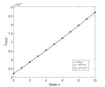
Figure 9: The total traces (probabilities) of the first 11 modes.

More explicitly, the transition probabilities of the first four modes are given by the following transmission matrix,

$$S =\begin{bmatrix}0.9838&0.0161&0.0000&0.0000\\ 0.0152&0.9538&0.0307&0.0003\\ 0.0001&0.0289&0.9266&0.0438\\ 0.0000&0.0003&0.0414&0.9018\end{bmatrix}.$$ (51)

Apparently, high-dimensional temporal modes can be sustained but their stabilities become low, i.e., the probabilities of transferring to other modes increases.

III.5 Entangled photon propagation

In this subsection, we will discuss the entangled photon pair propagation in a turbulence environment. To begin, we consider two entangled photons with the following initial state,

$$|\psi\rangle =\frac{1}{\sqrt{2}}(|f_{m}\rangle|f_{m}\rangle+|f_{n}\rangle|f_{n}\rangle),$$ (52)

Then, the reduced density operator is given by,

$$\rho^{i} =\frac{1}{2}\int\int\int\int[f_{m}(\omega_{1})f_{m}(\omega_{1}^{\prime})+f_{n}(\omega_{1})f_{n}(\omega_{1}^{\prime})]$$

$$\quad\cdot[f_{m}(\omega_{1})f_{m}(\omega_{1}^{\prime})+f_{n}(\omega_{2})f_{n}(\omega_{2}^{\prime})]$$

$$\quad\cdot|0_{\omega_{1}},0_{\omega^{\prime}_{1}}\rangle\langle 0_{\omega_{2}},0_{\omega^{\prime}_{2}}|d\omega_{1}d\omega_{1}^{\prime}d\omega_{2}d\omega_{2}^{\prime}.$$ (53)

We must adjust $l(z)$ to account for the cross terms $|0_{\omega_{1}},0_{\omega^{\prime}_{1}}\rangle\langle 0_{\omega_{2}},0_{\omega^{\prime}_{2}}|$$\ \left(\lambda_{i}=\frac{2\pi c}{\omega_{i}}\right)$

$$l(\omega_{1},\omega_{2},\omega_{1}^{\prime},\omega_{2}^{\prime},z) \approx\pi C_{n}^{2}(z)(\lambda_{1}\lambda_{2}){}^{-1}w_{0}^{-\frac{5}{3}}$$

$$\quad\cdot\bigg{\{}\left[1+\frac{1}{2}(\frac{\lambda_{1}z}{\pi w_{0}^{2}})^{2}+\frac{1}{2}(\frac{\lambda_{2}z}{\pi w_{0}^{2}})^{2}\right]^{\frac{5}{6}}$$

$$\quad+\left[1+\frac{1}{2}(\frac{\lambda^{\prime}_{1}z}{\pi w_{0}^{2}})^{2}+\frac{1}{2}(\frac{\lambda^{\prime}_{2}z}{\pi w_{0}^{2}})^{2}\right]^{\frac{5}{6}}\bigg{\}}.$$ (54)

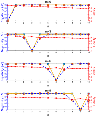
Figure 10: Negativity and fidelity with different modes .

In order to investigate the entanglement evolution of high dimensional entangled photon pairs in a random media, we choose the log negativity as an entanglement measure. Fig. (10) is plotted with the parameters $w_{0}=14.57\ \text{cm}$ and $z=30\ \text{km}$. We consider the strong turbulence case, which is characterized by $C_{n}^{2}=10^{-16}\ \text{m}^{-2/3}$ along the propagating path. We are interested in the robustness of entangled photon pairs under the influence of turbulence. To be more specific, we fix the mode number $m$ for one photon and vary the second photon’s mode number $n$ from 0 to 10. The blue squares are the negativities of the initial states and the red circles are the log negativities of the final states at the receiving aperture. Solid lines connect all the squares in every sub-figures where dash lines connect the circles. The red dot lines connect all the diagonal crosses are the fidelities between the initial states and the output states. We can see that, when the entangled photons propagate in a strong turbulence regime, the entanglement measured by the negativity defined as $E_{N}(\rho)=\log_{2}[2\mathcal{N}+1]$ doesn’t change too much. It’s easy to find that, when $m$ and $n$ are not close ($|m-n|>1$), the entanglement will remain unaffected even in a strong turbulence regime. When $|m-n|=1$, the two modes are close, interference occurs and heavily influences the log negativity. Thus, we show that the qudit formed by consecutive even number modes (e.g., modes 0, 2, 4) or odd number modes (e.g, modes 1, 3, 5) will be more robust against the random perturbations.

IV CONCLUSION

To summarize, based on the Schmidt decomposition representation, high dimensional temporal mode propagation is systematically studied by using the well-known infinitesimal propagation method. We have shown that, in a highly dynamic maritime environment, there exist frequency ranges that will allow the reliable implementations of photon communication in the framework of temporal modes. In particular, we have examined the feature of Schmidt eigenmodes and identified robust and fragile parameter domains against log-distance extinction (scattering and absorption). In addition, we have analysed the dynamical behavior of entangled photon pairs under the influence of strong turbulence. Since the colored noises and correlated noises are of importance for free-space communication, a further study on the photonic noisy propagation would be useful key-100 ; key-101 .

Appendix A Solutions of Integrals in IPE

The purpose of this Appendix is to analyze the influence of turbulence via infinitesimal propagation equation method. The generating function for the LG modes of a fixed wavelength can be written as

$$G =\sum_{n,m=0}^{\infty}\frac{1}{m!}L_{n}^{m}\left(\frac{2(u^{2}+v^{2})}{1+t^{2}}\right)\left[\frac{d(1+1t)}{1-it}\right]^{n}$$

$$\quad\times\frac{[(u+iv)p+(u-iv)q]^{m}}{(1-it)^{1+m}}$$

$$=\frac{1}{\Omega(t,d)}\exp\bigg{[}\frac{(u+iv)p}{\Omega(t,d)}+\frac{(u-iv)q}{\Omega(t,d)}$$

$$\quad-\frac{(1+d)(u^{2}+v^{2})}{\Omega(t,d)}\bigg{]},$$ (55)

where $\Omega(t,d)=1-d-it-itd.$ The normalized coordinates are given by $u=x/w_{0}$, $v=y/w_{0}$ and $t=z/z_{R}=z\lambda/\pi w_{0}^{2}$ in terms of the waist size $w_{0}$ at the initial location and the Rayleigh range $z_{R}$. The parameters $p$, $q$ and $w$ are used to generate particular LG modes in the following way,

$$M_{r,l}^{LG}(u,v,t) =\begin{cases}\mathcal{N}[\frac{1}{r!}\partial_{d}^{r}\partial_{p}^{|l|}G]_{d,p,q=0}&l>0\\ \mathcal{N}[\frac{1}{r!}\partial_{d}^{r}G]_{d,p,q=0}&l=0\\ \mathcal{N}[\frac{1}{r!}\partial_{d}^{r}\partial_{q}^{|l|}G]_{d,p,q=0}&l<0\end{cases}$$ (56)

with normalization constant

$$\mathcal{N} =\left[\frac{r!2^{|l|+1}}{\pi(r+|l|)}\right]^{\frac{1}{2}},$$ (57)

where $r$ is the radial index (a non-negative integer) and $l$ is the azimuthal index (an integer).

In order to compute the integrals in the IPE, we must get the the Fourier transform of the generating function,

$$\mathcal{F}[G] =\frac{\pi}{1+d}\exp[\frac{i\pi(\tilde{k}_{x}+i\tilde{k}_{y})p}{1+d}$$

$$\quad+\frac{i\pi(\tilde{k}_{x}-i\tilde{k}_{y})q}{1+d}-\frac{\pi(\tilde{k}_{x}^{2}+\tilde{k}_{y}^{2})\Omega(t,d)}{1+d}].$$ (58)

Here $\tilde{k}_{x}$ and $\tilde{k}_{y}$ are normalized spatial frequency components that $\tilde{k}_{x}=\frac{w_{0}}{2\pi}k_{x}$ and $\tilde{k}_{y}=\frac{w_{0}}{2\pi}k_{y}$.

After evaluating the Eq. (23) and removing the superfluous mixed terms containing a $p$ times a $q$, one obtains a generation function

$$S_{G}(z) =\frac{i\lambda(1+d_{m})(1+d_{n})}{8(1-d_{m}d_{n})}\exp\left[\frac{p_{m}p_{n}+q_{m}q_{n}}{2(1-d_{m}d_{n})}\right]$$

$$\quad\times[2(1-d_{m}d_{n})+p_{m}p_{n}+q_{m}q_{n}],$$ (59)

where $p_{m}$, $q_{m}$ and $d_{m}$ are generating function parameters associated with the $m$ index, while $p_{n}$, $q_{n}$ and $d_{n}$ are generating function parameters associated with the $n$ index. From this function, we find non-zero values occur when the azimuthal indices involved be equal, and that the radial indices differ at most by one, i.e., Eq. (32).

For the term $W_{m,n}(\mathbf{K},z)$ , we must to get a generating function for the radial indices of the modal correlation functions

$$W_{rG}(K,\phi,z) =\frac{\exp(-X)\exp[i(l_{m}-l_{n})\phi]E_{m}^{|l_{m}|}\bar{E}_{n}^{|l_{n}|}}{(1-d_{m}d_{n})}$$

$$\quad\times\left[\frac{r_{m}!}{(r_{m}+|l_{m}|)!}\right]^{\frac{1}{2}}\left[\frac{r_{n}!}{(r_{n}+|l_{n}|)!}\right]^{\frac{1}{2}}$$

$$\quad\times\sum_{s=0}^{M(l_{m},l_{n})}\frac{|l_{m}|!|l_{n}|!(-X)^{s}}{(|l_{m}|-s)!(|l_{n}|-s)!s!}$$ (60)

with

$$M(l_{m},l_{n}) =\frac{1}{2}(|l_{m}|+|l_{n}|-|l_{m}-l_{n}|),$$ (61)

$$X =\frac{K^{2}\zeta_{m}\zeta_{n}^{*}\eta^{2}}{8\pi^{2}(1-d_{m}d_{n})},$$ (62)

$$E_{m} =\frac{iK\zeta_{m}\eta}{2\sqrt{2}\pi(1-d_{m}d_{n})},$$ (63)

$$\bar{E}_{n} =\frac{iK\zeta_{n}^{*}\eta}{2\sqrt{2}\pi(1-d_{m}d_{n})}.$$ (64)

Here, we set $\zeta_{x}=z_{R}-iz-d_{x}(z_{R}+iz)$, $\eta=\frac{\lambda}{w_{0}}$, and use we are using polar momentum space coordinates $k_{x}+ik_{y}=Ke^{i\phi}$ . Setting $a=(1+t^{2})w_{0}{}^{2},b=\frac{1+it}{1-it}$,we can get $X=\frac{K^{2}(1-d_{m}b)(1-d_{n}b^{-1})a}{8(1-d_{m}d_{n})}$, and the explicit form of the term $W_{m,n}(K,\phi,z)$ can be written as

$$W_{m,n}(K,\phi,z) =\sum_{s=0}^{M(l_{m},l_{n})}e^{i(l_{m}-l_{n})\phi}(i)^{|lm|+|l_{n}|}(-1)^{-s}\left(\frac{K^{2}a}{8}\right)^{\frac{|l_{m}|+|l_{n}|}{2}-s}\left[\frac{1}{(r_{m}+|l_{m}|)!}\right]^{\frac{1}{2}}\left[\frac{1}{(r_{n}+|l_{n}|)!}\right]^{\frac{1}{2}}$$

$$\quad\times\frac{|l_{m}|!|l_{n}|!}{(|l_{m}|-s)!(|l_{n}|-s)!s!}b^{-\frac{|l_{m}|-|l_{n}|}{2}}\partial_{d_{m}}^{r_{m}}\partial_{d_{n}}^{r_{n}}\left(e^{-X}\frac{(1-d_{m}b)^{|l_{m}|-s}(1-d_{n}b^{-1})^{|l_{n}|-s}}{(1-d_{m}d_{n})^{|l_{m}|+|l_{n}|-s+1}}\right)\Bigg{|}_{d_{m},d_{m}=0},$$ (65)

which can also be sorted as

$$W_{m,n}(K,\phi,z) =\sum_{j=0}^{\infty}c_{m,n,j}\left(\frac{K^{2}a}{8}\right)^{\frac{j}{2}}e^{-\frac{K^{2}a}{8}}e^{i(l_{m}-l_{n})\phi},$$ (66)

where $c_{m,n,j}$ is a coefficient independent of $K$ and $\phi$.

When we substitute the von Karman spectrum, the two-dimensional integration in Eq. (40) can be split into a radial and angular integral. Since the von Karman density $\Phi_{1}(K)$ only depends on the radial coordinate, the integral over $\phi$ only involves the $\phi$ component of $W_{m,n}$. Non-zero values only occur when $l_{m}-l_{u}-l_{n}+l_{v}=0$. Setting $\kappa_{0}\rightarrow 0$, we can get

$$L_{m,n,u,v}(z) =k^{2}\int\Phi_{1}(\mathbf{K})W_{m,u}(\mathbf{K},z)W_{n,v}^{*}(\mathbf{K},z)\frac{d^{2}K}{4\pi^{2}}$$

$$\approx\delta_{mu}\delta_{n\nu}L_{T}+(8.1)\delta_{l_{m}-l_{u},l_{n}-l_{v}}C_{n}^{2}\lambda^{-2}w_{0}^{\frac{5}{3}}(1+t^{2})^{\frac{5}{6}}\left\{\sum_{j_{1},j_{2}=0}^{\infty}2^{-\frac{j_{1}+j_{2}}{2}}\Gamma\left[\frac{j_{1}+j_{2}}{2}-\frac{5}{6}\right]c_{m,u,j_{1}}c_{n,v,j_{2}}^{*}\right\}.$$ (67)

References

- (1) C. Weedbrook, S. Pirandola, R. García-Patrón, N. J. Cerf, T. C. Ralph, J. H. Shapiro, and S. Lloyd, Rev. Mod. Phys. 84, 621 (2012).
- (2) C. H. Bennett and G. Brassard, IEEE New York (1984).
- (3) N. Gisin, G. Ribordy, W. Tittel, and H. Zbinden, Rev. Mod. Phys. 74, 145 (2002).
- (4) K. Bartkiewicz, A. Černoch, K. Lemr, A. Miranowicz, and F. Nori, Phys. Rev. A 93, 062345 (2016).
- (5) A. K. Ekert, Phys. Rev. Lett. 67, 661 (1991).
- (6) Kimble, H. J., Nature 453, 1023 - 1030 (2008).
- (7) J. I. Cirac, P. Zoller, H. J. Kimble, and H. Mabuchi, Phys. Rev. Lett. 78, 3221-3224 (1997).
- (8) A. Reiserer, N. Kalb, G. Rempe, and S. Ritter, Nature (London) 508, 237 (2014).
- (9) H.-K. Lo and H. F. Chau, Science 283, 2050 (1999).
- (10) P. W. Shor and J. Preskill, Phys. Rev. Lett. 85, 441 (2000).
- (11) H.-K. Lo, X. Ma, and K. Chen, Phys. Rev. Lett. 94, 230504 (2005).
- (12) N. J. Cerf, M. Bourennane, A. Karlsson, and N. Gisin, Phys. Rev. Lett. 88, 127902 (2002).
- (13) G. Brassard, A. Nayak, A. Tapp, D. Touchette, and F. Unger, 2014 IEEE 55th Annual Symposium on Foundations of Computer Science, 296305 (2014).
- (14) S. J. van Enk, J. I. Cirac, and P. Zoller, Phys. Rev. Lett. 78, 4293 (1997).
- (15) G. Vallone, V. D’Ambrosio, A. Sponselli, S. Slussarenko, L. Marrucci, F. Sciarrino, and P. Villoresi, Phys. Rev. Lett. 113, 060503 (2014).
- (16) A. Mair, A. Vaziri, G. Weihs, and A. Zeilinger, Nature (London) 412, 313 (2001).
- (17) G. Gibson, J. Courtial, M. J. Padgett, M. Vasnetsov, V. Pasko, S. M. Barnett, and S. Franke-Arnold, Opt. Express 12, 5448 (2004).
- (18) J. Wang, J.-Y. Yang, I. M. Fazal, N. Ahmed, Y. Yan, H. Huang, Y. Ren, Y. Yue, S. Dolinar, M. Tur, and A. E. Willner, Nat. Photon. 6, 488 (2012).
- (19) M. Agnew, J. Leach, M. Mclaren, F. S. Roux, and R. W. Boyd, Phys. Rev. A 84, 062101 (2011).
- (20) M. Mafu, A. Dudley, S. Goyal, D. Giovannini, M. Mclaren, M. J. Padgett, T. Konrad, F. Petruccione, N. Lütkenhaus, and A. Forbes, Phys. Rev. A 88, 032305 (2013).
- (21) M. Mirhosseini, O. S. Magaña-Loaiza, M. N. O’Sullivan, B. Rodenburg, M. Malik, M. P. J. Lavery, M. J. Padgett, D. J. Gauthier, and R. W. Boyd, New J. Phys. 17, 033033 (2015).
- (22) B. Brecht, D. V. Reddy, C. Silberhorn, and M. Raymer, Phys. Rev. X 5, 041017 (2015).
- (23) M. Pant and D. Englund, Phys. Rev. A 93, 043803 (2016).
- (24) P. Manurkar, N. Jain, M. Silver, Y.-P. Huang, C. Langrock, M. M. Fejer, P. Kumar, and G. S. Kanter, Optica 3, 1300 (2016).
- (25) T. Zhong, H. Zhou, R. D. Horansky, C. Lee, V. B. Verma, A. E. Lita, A. Restelli, J. C. Bienfang, R. P. Mirin, T. Gerrits, S. W. Nam, F. Marsili, M. D. Shaw, Z. Zhang, L. Wang, D. Englund, G. W. Wornell, J. H. Shapiro, and F. N. C. Wong, New J. Phys. 17, 022002 (2015).
- (26) Z. Zhang, J. Mower, D. Englund, F. N. C. Wong, and J. H. Shapiro, Phys. Rev. Lett. 112, 120506 (2014).
- (27) J. Mower, Z. Zhang, P. Desjardins, C. Lee, J. H. Shapiro, and D. Englund, Phys. Rev. A 87, 062322 (2013).
- (28) U. S. Atmosphere, National Aeronautics and Space Administration, United States Air Force, Washington, DC (1976).
- (29) W. J. Wiscombe, Appl. Opt. 19, 1505 (1980).
- (30) C. Mätzler, IAP Res. Rep 8, 1 (2002).
- (31) H. E. Gerber, Relative-humidity parameterization of the Navy Aerosol Model (NAM) (1985).
- (32) A. M. J. V. Eijk and D. L. Merritt, Atmospheric Optical Modeling, Measurement, and Simulation II (2006).
- (33) D. C. Burnham and D. L. Weinberg, Phys. Rev. Lett. 25, 84 (1970).
- (34) L. Allen, M. W. Beijersbergen, R. J. C. Spreeuw, and J. P. Woerdman, Phys. Rev. A 45, 8185 (1992).
- (35) C. K. Law and J. H. Eberly, Phys. Rev. Lett. 92, 127903 (2004).
- (36) C. K. Law, I. A. Walmsley, and J. H. Eberly, Phys. Rev. Lett. 84, 5304 (2000).
- (37) F. S. Roux, Phys. Rev. A 83, 053822 (2011); F. S. Roux, Phys. Rev. A 88, 049906(E) (2013).
- (38) F. S. Roux, J. Phys. A: Math. Theor. 47, 195302 (2014).
- (39) F. S. Roux, J. Opt. 18, 055203 (2016).
- (40) P. A. Frederickson, K. L. Davidson, C. R. Zeisse, and C. S. Bendall, J. Appl. Meteor. 39, 1770 (2000).
- (41) P. A. Frederickson, S. Hammel, and D. Tsintikidis, Atmospheric Optical Modeling, Measurement, and Simulation II (2006).
- (42) J. Jing, T. Yu, Phys. Rev. Lett. 105, 240403 (2010); J. Jing, L.A. Wu, M. Byrd, J. Q. You, T. Yu, and Z.M. Wang, Phys. Rev, Lett. 114, 190502 (2015).
- (43) J. Jing, R. Li, J.Q. You, and T. Yu, Phys. Rev. A 91, 022109 (2015).