Optimal transport on large networks
a practitioner’s guide

Abstract

This article presents a set of tools for the modeling of a spatial allocation problem in a large geographic market and gives examples of applications. In our settings, the market is described by a network that maps the cost of travel between each pair of adjacent locations. Two types of agents are located at the nodes of this network. The buyers choose the most competitive sellers depending on their prices and the cost to reach them. Their utility is assumed additive in both these quantities. Each seller, taking as given other sellers prices, sets her own price to have a demand equal to the one we observed. We give a linear programming formulation for the equilibrium conditions. After formally introducing our model we apply it on two examples: prices offered by petrol stations and quality of services provided by maternity wards. These examples illustrate the applicability of our model to aggregate demand, rank prices and estimate cost structure over the network. We insist on the possibility of applications to large scale data sets using modern linear programming solvers such as Gurobi. In addition to this paper we released a R toolbox to implement our results and an online tutorial.

1 Introduction

The recent literature made an extensive use of networks to model market structure. However the scalability of these models is limited by the difficulty to compute equilibrium on large data sets. The results are therefore dependent on possible edge effects. In this paper, we present a set of tools to solve this issue and compute equilibrium of spatial allocation problems in large geographic markets. In our model we consider two types of agents, buyers and sellers, whose locations are fixed. The market is modeled by a network that maps travel costs between two adjacent locations. Buyers choose the most competitive seller depending on their prices and the cost to reach them. Each seller, taking as given other sellers prices, sets his own price to have a demand equal to the one we observed. Under a linear programming framework, the equilibrium is shown to be equivalent to a minimum cost flow. This problem is a compact formulation of the matching problem between buyers and sellers. After proving the existence of an equilibrium, we discuss the question of uniqueness.

We illustrate the applicability of this model on two examples. In the first one, knowing the prices set by gas stations and the distribution of consumers over the market, we aggregate the demand at each station and plot their geographic market share. The second example discusses the competition between maternity wards over the quality of services provided. Taking as given the location of households expecting a baby and the number of births in each hospital, we infer a ranking of maternity wards. For both of these examples we discuss our results and the limits of our model. In addition to this paper we released a R toolbox and an online tutorial to simplify the application of these methods to economic problems.

Relation to literature

Linear programming was pioneered by Kantorovich and Koopmans with applications for the computation of economic optimum. In parallel, Hitchcock formulated transportation problems as linear programs. Dantzig developed the general framework for linear programming problems and introduced the simplex method to solve them. We can note that from the very beginning, both optimal transportation problems and optimum of economic problems were the two important main applications of this problem. This paper presents linear programming solvers that were recently developed and can solve large scale problems. We defend the idea that these tools renew the interest for a linear programming formulation of economic problems.

Linear programming problems focus on the question of the economic optimum whereas economic theory is more interested by economic equilibrium. In matching markets with non-transferable (Gale and Shapley,, 1962) and transferable utility (Shapley and Shubik,, 1971) equilibrium is defined using the notion of pairwise stability. The duality theory of linear programming shows that, when utility is transferable, the solution of the optimization problem is an equilibrium.

Optimal transport problems were originally introduced by Monge and solved by Kantorovich. More recently, Bertsekas, (1998) studied optimal transport on networks and proposed several algorithms to compute a solution. This theory is also developed in the literature about the applications of optimal transport (Santambrogio,, 2015; Galichon,, 2016). Several of these results started being used in recent developments of the trade literature: Eaton and Kortum, (2002) developed quantitative versions of the Armington trade models allowing counterfactuals with respect to trade costs in a multicountry competitive equilibrium. Following this work, Allen and Arkolakis, (2014), Allen et al., (2015) and Allen and Arkolakis, (2016) computed the first-order welfare impact of reductions to the cost of shipping across specific links in an Armington model but did not optimize over the space of networks. Fajgelbaum and Schaal, (2017) keep developing these models and make the connection with the optimal transport theory, solving a global optimization over the space of networks in a neoclassical framework. The dimensions of the problems considered in these models remain however limited.

2 Model

Settings

The geometry of the geographic market is described by a connected graph $G=\left(V,E\right)$ with $V$ a set of vertices and $E$ a set of directed edges. Vertices are the different locations; edges are road segments linking two adjacent locations. Agents are located at the vertices of our graph. We make the following assumptions on their consumption preferences:

(A1)

Consumers with the same location have the same outside option.

(A2)

Consumers have the same cost of travel along a given edge.

(A3)

There is no capacity constraints on the supply side.

We will discuss in the next paragraph how these assumptions can be relaxed. However they seem to be realistic on several markets and in particular on both examples presented in this paper. They aim at simplifying the computation of equilibria in large scale markets.

A path $\pi_{vw}$ between two nodes $v,w\in V$ is a sequence of connected edges starting in $v$ and ending in $w$. We note $\Pi_{vw}$ the set of paths between $v$ and $w$. As $G$ is a connected graph, the set of paths between any pair of nodes is not empty.

For each edge $e\in E$, we define $c_{e}$ the cost of travel along this arc. A seller located in $w\in V$ sells at an endogenous price $p_{w}$. Therefore a consumer located in $v$ chooses to buy from the seller located in $w$ that minimizes his total cost $p_{v}$:

$$p_{v}=\underset{w\in V\text{, }\pi_{vw}\in\Pi_{vw}}{\min}\left[p_{w}+\underset{e\in\pi_{vw}}{\sum}c_{e}\right]$$

Let’s denote $u_{v}$ the reservation utility of agents located in $v$ and $p_{v}$ the price for these agents (including the cost of transportation). Therefore, if $p_{v}>u_{v}$ a consumer in $v$ chooses his outside option, else he buys from the most competitive seller depending on his location in the market. This outside option can be modeled by a fictitious node $0$, where the price of the commodity is set to $p_{0}=0$ and the cost of travel is $c_{v0}=u_{v}$. Hence the excess demand $z_{v}$ at a node $v\in V$ does not depend on the price.

We are solving a matching problem over a network between sellers and consumers. At equilibrium each consumer chooses the most competitive seller depending on his location; furthermore the demand received by each seller must equal his supply. If we define $\mu_{e}$ the number of agents traveling along edge $e$, these equilibrium conditions can be written:

$$\left\{\begin{array}[]{l}\forall vw\in E\text{, }p_{w}-p_{v}\leq c_{vw}\\ \forall vw\in E\text{ such that }\mu_{vw}>0\text{, }p_{w}-p_{v}=c_{vw}\\ \forall v\in V\text{, }\underset{w\in V}{\sum}\mu_{vw}-\underset{u\in V}{\sum}\mu_{uv}=z_{v}\end{array}\right.$$

These equations are the complementary slackness conditions for a minimum cost flow problem over $G$. Hence, if the graph is connected and if there isn’t any loop of negative cost in $G$, there exists an equilibrium which is the solution of the min-cost flow problem

$$\begin{array}[]{cl}\mu=\arg&\min\underset{e\in E}{\sum}c_{e}\mu_{e}\\ &\mu\text{ s.t. }\forall v\in V\text{, }\underset{w\in V}{\sum}\mu_{vw}-\underset{u\in V}{\sum}\mu_{uv}=z_{v}\end{array}$$

Degeneracy

The optimal transport problem of Monge-Kantorovich is known for having degenerated solutions. In economic terms this means that prices are going to make consumers indifferent between several sellers. A power diagram, also called Laguerre-Voronoi, is a partition of the space that maps the geographic market shares of sellers. The non-uniqueness of power diagrams is a consequence of the degeneracy of solutions to the optimal transport problem. In this paragraph we explained how the degeneracy can be mitigated at the price of some efficiency of computation.

Consider for example the following market:

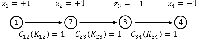
Figure 2.1: Example of market with degenerated solutions

Buyers are located in nodes 1 and 2 and sellers in nodes 3 and 4. At equilibrium $p_{4}=p_{3}+1$ and buyers are indifferent between both sellers. Hence two degenerated power diagrams coexist as well as any convex combination of both.

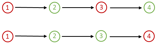
Figure 2.2: Example of degenerated power diagrams

One way to mitigate this problem and select the relevant power diagrams is to alter the cost of travel for agents. Let’s consider that consumers located is $v\in V$ solve the problem:

$$p_{v}=\underset{w\in V\text{, }\pi_{vw}\in\Pi_{vw}}{\min}\left[p_{w}+\left(\underset{e\in\pi_{vw}}{\sum}c_{e}\right)^{\alpha}\right]$$

If $\alpha>1$ consumers value more the cost of closer arcs than the ones that are further.

As the initial position of each agent matters, the equilibrium conditions won’t be the same as before. We now face a classical matching problem with transferable utility. The computation of the equilibrium requires first to calculate the geodesic distances between each pair of consumer and seller. In the case of the example above, the problem becomes:

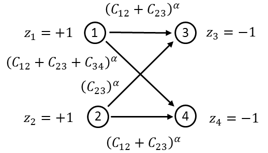
Figure 2.3: Solving the degeneracy problem

Depending on the value of $\alpha$ we get a different power diagram and solve the degeneracy problem at the price of increasing significantly the dimensions of the problem. The network is less sparse than it was and we have to solve a shortest past problems for each pair of agents before solving the matching problem.

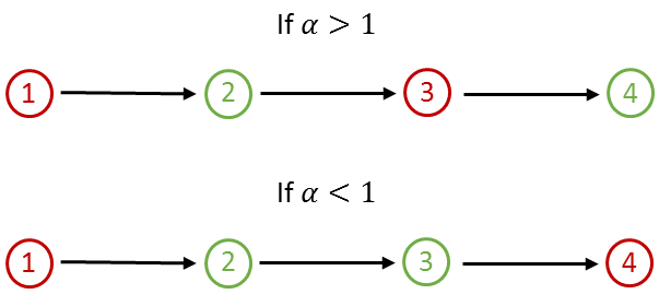
Figure 2.4: Non-degenerated power diagrams

Build a geographic network

The shapefile format is a normalized data format used by geographic information system software. It spatially describes vector features (points, lines and polygons) representing for example roads, lakes or facilities. Each of these elements is associated with a vector of characteristics that describes it. Several open source data sets describing France geographic characteristics are distributed by the IGN (Institut Geographic National) under a shapefile format. The examples treated in this paper use the route500 dataset that describes 500 000 km of roads.

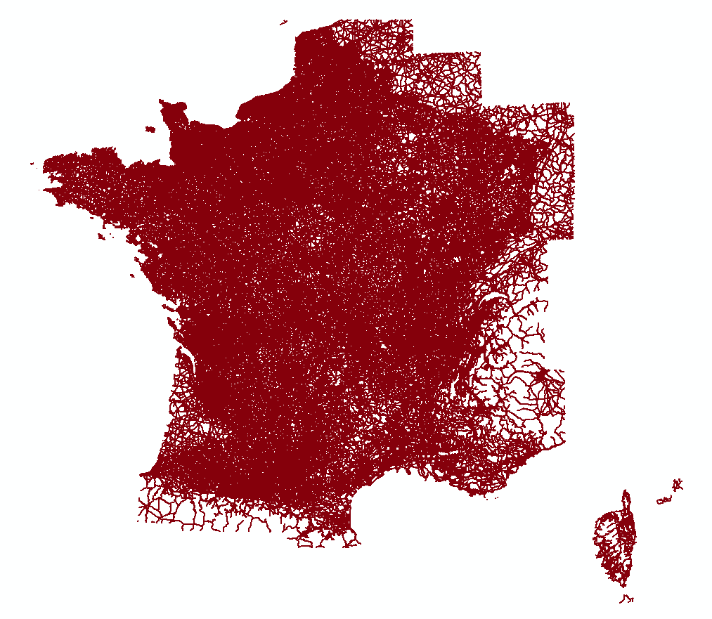
Figure 2.5: Example of shapefile: the route500 data set

We released a R toolbox that generates a network from a shapefile and compute an equilibrium for the spatial matching problem described above. Thus, the route500 dataset is converted in a directed graph which contains 186 464 nodes and 583 550 arcs after simplification and after retaining the largest connex subgraph. This graph maps the french road network and the locations of our agents. Each node and arc is associated with a vector of characteristics such as road type, distance between extremities or administrative area. The following figure shows the position of nodes within Paris.

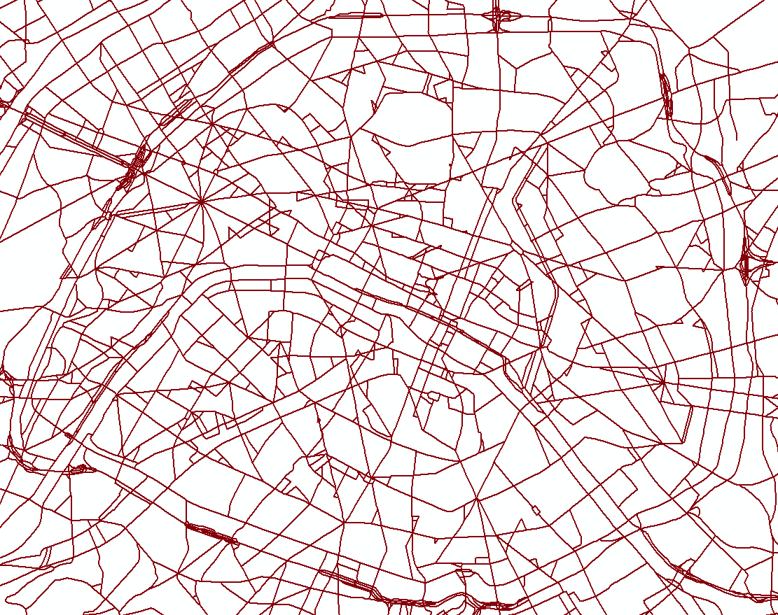
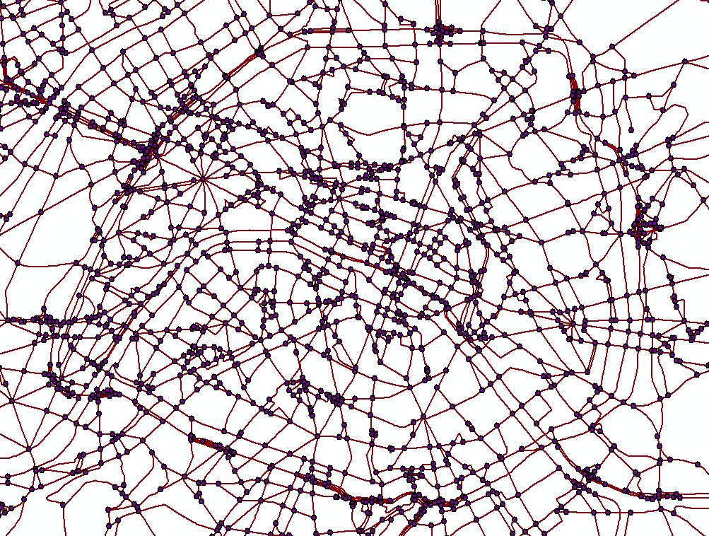
Figure 2.6: From a shapefile to a geographic network

The toolbox uses Gurobi, a particularly efficient linear programming solver, to compute an equilibrium. For the network described above and without parallel computing, it returns an equilibrium solution in a few seconds. In addition to this toolbox, we also released a comprehensive online tutorial that goes through the examples presented in the last part of this paper and describes the details of the computations.

Iceberg costs

Models used in trade theory usually use iceberg transport costs. These costs are linear in distance and paid in the transported good once arrived - hence the metaphor of the iceberg that melts as you transport it. Our model can incorporate these costs applying a log-transformation to the equilibrium conditions.

Let’s define for all $vw\in E$ iceberg costs $\tau_{vw}$. An equilibrium $\left(\mu,p\right)$ should satisfy

$$\left\{\begin{array}[]{l}\forall vw\in E\text{, }\left(1-\tau_{vw}\right)p_{w}\leq p_{v}\\ \forall vw\in E\text{ such that }\mu_{vw}>0\text{, }\left(1-\tau_{vw}\right)p_{w}=p_{v}\\ \forall v\in V\text{, }\underset{w\in V}{\sum}\mu_{vw}-\underset{u\in V}{\sum}\mu_{uv}=z_{v}\end{array}\right.$$

which becomes

$$\left\{\begin{array}[]{l}\forall vw\in E\text{, }\log p_{w}-\log p_{v}\leq-\log\left(1-\tau_{vw}\right)\\ \forall vw\in E\text{ such that }\mu_{vw}>0\text{, }\log p_{w}-\log p_{v}=-\log\left(1-\tau_{vw}\right)\\ \forall v\in V\text{, }\underset{w\in V}{\sum}\mu_{vw}-\underset{u\in V}{\sum}\mu_{uv}=z_{v}\end{array}\right.$$

Therefore this problem is equivalent to the one presented in the first paragraph of this section with $\forall vw\in E$, $c_{vw}=-\log\left(1-\tau_{vw}\right)$ and replacing $p$ by its logarithm.

Population heterogeneity

The model can be altered to take into account some heterogeneity of the agents. For example, if agents located a same node have different reservation utility, this specific node can be replaced by two different locations with the same connections to the rest of the network but with different costs of transportation toward the node 0. Following the same idea, we can model heterogeneity in the costs of transportation across agents by duplicating some parts of the network.

3 Applications to economic modeling

As emphasize previously, the main interest of this model is its tractability and our ability to compute solutions when its dimensions become large. One difficulty we faced when we looked for examples to apply it, was the difficulty to find disaggregated data. In this section, we focus on two examples: prices offered by petrol stations and quality of services provided by maternity wards. The first example is not new in the economic literature and has been studied in Borenstein et al., (1997) and in Eckert and West, (2004).

Aggregate the demand

Assume we know the cost of transportation, the locations of agents and the prices set by sellers. To compute the demand served by each seller we have to solve the discrete choice problem faced by consumers. The result can be plotted on a power diagram that represents the geographic market shares of each seller.

Let’s consider the gas retail market in France. Gas stations, which are on the supply side of this market, are assigned to the closest node in the network built in the last section. The following figure plots their locations and prices (the greener is a dot, the cheaper is the price).

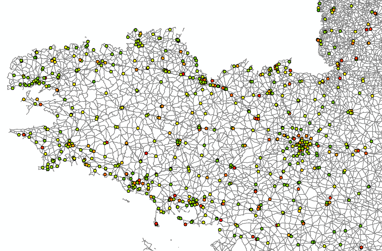
Figure 3.1: Gas stations: location and price

Our proxy for the demand is the localized calls of the mobile application mon-essence.fr. This application, installed on 1 to 5 millions android mobiles, gives the prices in petrol stations that are close to your location. We assume that each consumer wants to buy the same quantity of fuel. This gives the following distribution of demand within the market. Some criticisms can be made on this proxy and we can in particular emphasize the risk of selection bias. As we don’t know the characteristics of the population that installed this application, we can’t control for this issue.

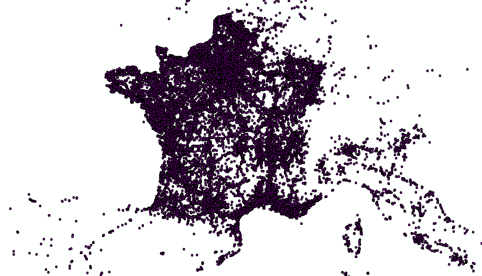
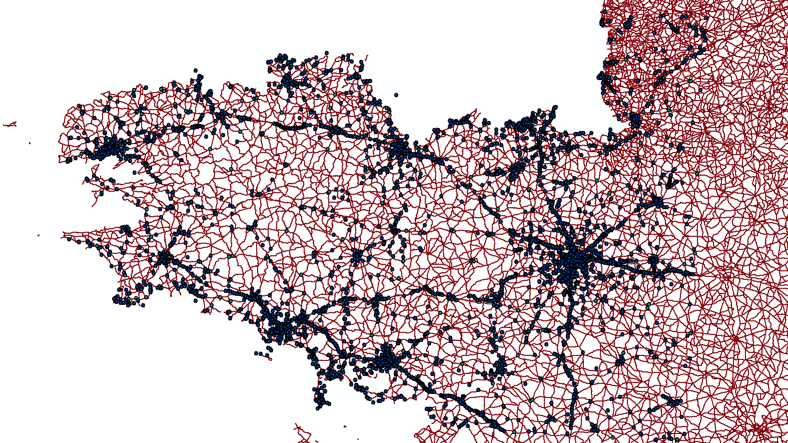
Figure 3.2: Proxy for gas demand - France and Brittany

Finally, in order to compute the demand received by each gas station, we need to assume a cost structure over the network. Here we multiply the geographic distance between the two extremities of an arc by a cost per kilometer. Obviously we could use other characteristics of the edges such as the type of roads for example.

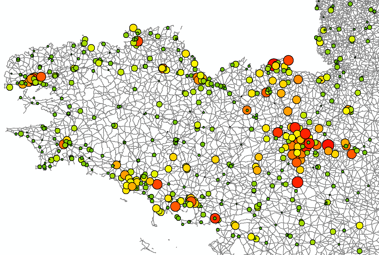
Figure 3.3: Demand received by each gas station

On smaller network, we can also plot the geographic market share of each seller on a power diagram. The network structure may strongly influence the shape and results we get.

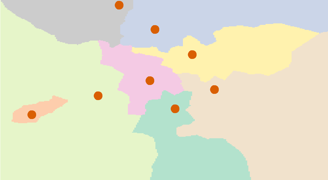
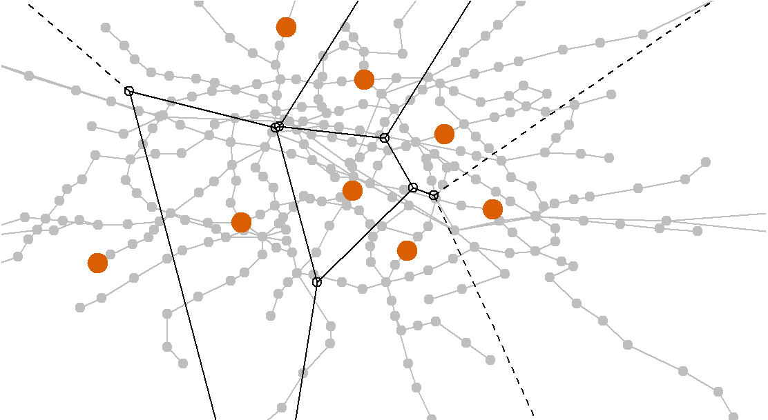
Figure 3.4: Power diagrams with and without network

We can emphasize several limitations of the model. As said before, this example was aiming at illustrating how one can find the demand received by each seller knowing locations of consumers, prices and travel costs. Here we make strong assumptions on the structure of those three variables that should be more carefully discussed. The fact that all consumers are willing to buy the same quantity of gasoline is a particularly strong assumption. We should justify precisely the use of our proxy for demand distribution and the travel costs structure. Finally to avoid edge effects, we should not interpret results at locations close to the borders of the network.

Rank the quality of service

Health care costs are regulated in France and public hospitals can’t choose the price they charge. Patients choose their hospitals depending on the travel cost and the quality of service provided. Hence the prices we were considering in the last example are now the opposite of an index for quality of service.

We know the location of pregnant households and the number of births in each maternity ward and want to infer a ranking of hospitals. Once again, we assume that travel cost along an edge is proportional with its length. Because we only care about the order of maternity wards ranked over their quality of service, the unit of the cost of transportation does not matter.

We use the SAE data set (Statistiques Annuelles des Etablissements) describing maternity wards in France. For each of them, we have its location, the number of beds available, the number of workers in the hospital, the number of births and the number of voluntary interruptions of pregnancy per year. We cross this data set with the INSEE database to get the number of mothers giving birth per administrative unit between 2004 and 2014. We plot these data on the following figure. On the left we draw the locations of maternity wards in France and on the right the number of births per administrative unit in Paris, in Ile-de-France and in Brittany.

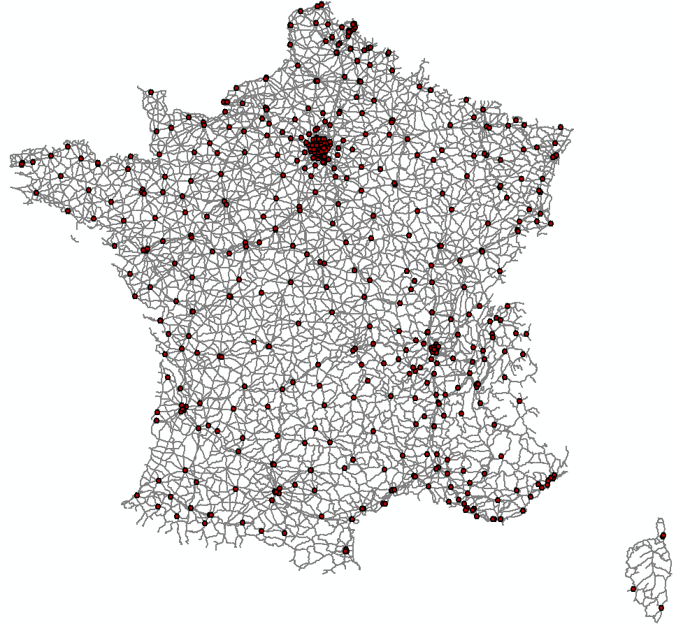
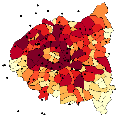
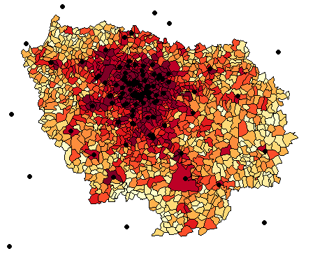
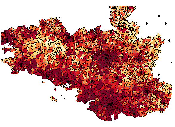
Figure 3.5: Location of maternity wards in France and number of births within administrative units in Paris, in Ile-de-France and in Brittany

Within a given administrative area, we consider the number of roads intersections as a reasonable proxy for the density of population. Therefore, the population in an administrative unit is divided between the different nodes inside this area.

One difficulty we met is the existence of outside options such as private or foreign hospitals. We chose the arbitrary convention to locally balance supply and demand - and therefore remove agents that are using their outside options - over five geographic areas: North-West, North-East, South-West, South-East and Paris area. We solve the associated min-cost flow problem and plot the ranking of maternity wards on the following figure.

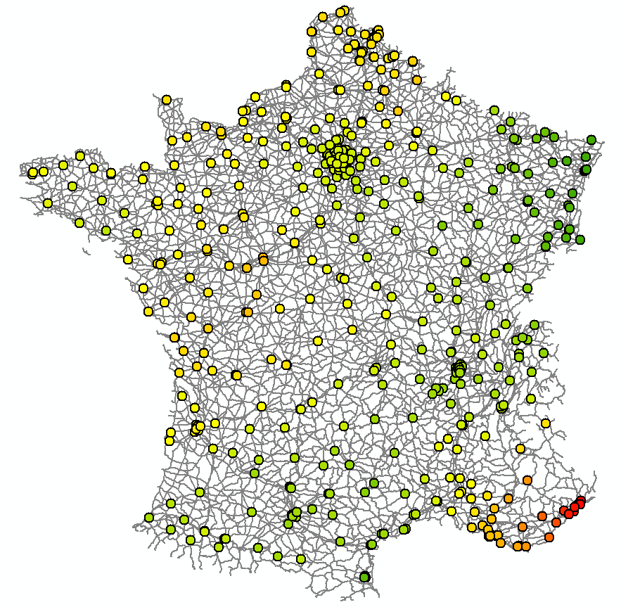
Figure 3.6: Quality of services in maternity wards

We see two main limitations to this model. Maternity wards may face binding capacity constraints such as number of doctors or available beds. We would also need additional data on the localization of outside options such as private hospitals or information to remove agents using their outside option from our data set.

4 Conclusion

In this paper we present a set of tools for the economic modeling of matching problems between two types of agents located on a large geographic market. We believe that the recent development of efficient linear programming solvers such as Gurobi could renew the interest of economists for these methods.

The modeling of a geographic market as a network seems relevant but also practical and efficient when dimensions become large. This efficiency is a consequence of the natural sparsity of roads network but also a consequence of the strong assumptions of the model such as linear costs of transport and additive utility. Whereas this assumptions obviously brings limitations, we consider that the advantages of tractability exceed them.

The examples presented in the paper are in line with this idea. The difficulty to find disaggregated data on large geographic market make us focus on two different examples: the gas retail market and the maternity wards. We used these examples to present several applications such as the computation of demand received by each gas retailer and the ranking of the quality of service in maternity wards.

In addition to this paper we released a R toolbox to implement our results and an online tutorial.

References

- Allen and Arkolakis, (2014) Allen, T. and Arkolakis, C. (2014). Trade and the topography of the spatial economy. The Quarterly Journal of Economics, 129(3):1085–1140.
- Allen and Arkolakis, (2016) Allen, T. and Arkolakis, C. (2016). The welfare effects of transportation infrastructure improvements. Manuscript, Dartmouth and Yale.
- Allen et al., (2015) Allen, T., Arkolakis, C., and Li, X. (2015). On the existence and uniqueness of trade equilibria. Manuscript, Yale Univ.
- Bertsekas, (1998) Bertsekas, D. P. (1998). Network optimization: continuous and discrete models. Citeseer.
- Borenstein et al., (1997) Borenstein, S., Cameron, A. C., and Gilbert, R. (1997). Do gasoline prices respond asymmetrically to crude oil price changes? The Quarterly journal of economics, 112(1):305–339.
- Eaton and Kortum, (2002) Eaton, J. and Kortum, S. (2002). Technology, geography, and trade. Econometrica, 70(5):1741–1779.
- Eckert and West, (2004) Eckert, A. and West, D. S. (2004). Retail gasoline price cycles across spatially dispersed gasoline stations. The Journal of Law and Economics, 47(1):245–273.
- Fajgelbaum and Schaal, (2017) Fajgelbaum, P. D. and Schaal, E. (2017). Optimal transport networks in spatial equilibrium. Technical report, National Bureau of Economic Research.
- Gale and Shapley, (1962) Gale, D. and Shapley, L. S. (1962). College admissions and the stability of marriage. The American Mathematical Monthly, 69(1):9–15.
- Galichon, (2016) Galichon, A. (2016). Optimal Transport Methods in Economics. Princeton University Press.
- Heijnen and Soetevent, (2014) Heijnen, P. and Soetevent, A. R. (2014). Price competition on graphs.
- Maskin and Tirole, (1988) Maskin, E. and Tirole, J. (1988). A theory of dynamic oligopoly, ii: Price competition, kinked demand curves, and edgeworth cycles. Econometrica: Journal of the Econometric Society, pages 571–599.
- Pálvölgyi, (2011) Pálvölgyi, D. (2011). Hotelling on graphs. Technical report, Mimeo.
- Pinkse et al., (2002) Pinkse, J., Slade, M. E., and Brett, C. (2002). Spatial price competition: a semiparametric approach. Econometrica, 70(3):1111–1153.
- Santambrogio, (2015) Santambrogio, F. (2015). Optimal transport for applied mathematicians. Birkäuser, NY.
- Shapley and Shubik, (1971) Shapley, L. S. and Shubik, M. (1971). The assignment game i: The core. International Journal of game theory, 1(1):111–130.