Sampling the $\mu\nu$SSM for displaced decays of the tau left sneutrino LSP at the LHC

Abstract

Within the framework of the $\mu\nu{\rm SSM}$, a displaced dilepton signal is expected at the LHC from the decay of a tau left sneutrino as the lightest supersymmetric particle (LSP) with a mass in the range $45-100$ GeV. We compare the predictions of this scenario with the ATLAS search for long-lived particles using displaced lepton pairs in $pp$ collisions, considering an optimization of the trigger requirements by means of a high level trigger that exploits tracker information. The analysis is carried out in the general case of three families of right-handed neutrino superfields, where all the neutrinos get contributions to their masses at tree level. To analyze the parameter space, we sample the $\mu\nu$SSM for a tau left sneutrino LSP with proper decay length $c\tau>0.1$ mm using a likelihood data-driven method, and paying special attention to reproduce the current experimental data on neutrino and Higgs physics, as well as flavor observables. The sneutrino is special in the $\mu\nu{\rm SSM}$ since its couplings have to be chosen so that the neutrino oscillation data are reproduced. We find that important regions of the parameter space can be probed at the LHC run 3.

Keywords: Supersymmetry Phenomenology; Supersymmetric Standard Model; LHC phenomenology

1 Introduction

The search for low-energy supersymmetry (SUSY) is one of the main goals of the LHC. This search has been focused mainly on signals with missing transverse energy (MET) inspired in $R$-parity conserving (RPC) models, such as the minimal supersymmetric standard model (MSSM) [1, 2, 3]. There, significant bounds on sparticle masses have been obtained [4], especially for strongly interacting sparticles whose masses must be above about 1 TeV [5, 6]. Less stringent bounds of about 100 GeV have been obtained for weakly interacting sparticles, and even the bino-like neutralino is basically not constrained due to its small pair production cross section. Qualitatively similar results have also been obtained in the analysis of simplified $R$-parity violating (RPV) scenarios with trilinear lepton- or baryon-number violating terms [7], assuming a single channel available for the decay of the LSP into leptons. However, this assumption is not possible in other RPV scenarios, such as the ‘$\mu$ from $\nu$’ supersymmetric standard model ($\mu\nu{\rm SSM}$) [8], where the several decay branching ratios (BRs) of the LSP significantly decrease the signal. This implies that the extrapolation of the usual bounds on sparticle masses to the $\mu\nu{\rm SSM}$ is not applicable.

The most recent analyses of signals at the LHC for LSP candidates in the $\mu\nu{\rm SSM}$ have been dedicated to the left sneutrino [9, 10], and to the bino-like neutralino [11]. In the latter case, it was shown that no points of the parameter space of the $\mu\nu{\rm SSM}$ were excluded when the left sneutrino is the next-to-LSP (NLSP) and hence a suitable source of binos. In the region of bino (sneutrino) masses $110-120$ ($120-140$) GeV it was found a tri-lepton signal compatible with the local excess reported by ATLAS [18]. If this excess were due to a statistical fluctuation, the prospects for the bounds on the parameter space of the sneutrino-bino mass in the $\mu\nu{\rm SSM}$ were discussed for the 13-TeV search with an integrated luminosity of 100 and 300 fb^-1.

Concerning the left sneutrino LSP, in Ref. [9] the prospects for detection of signals with di-photon plus leptons or MET from neutrinos, and multi-leptons, from the pair production of left sneutrinos/sleptons and their prompt decays ($c\tau\raise 1.29167pt\hbox{$\;<$\kern-7.5pt\raise-4.73611pt\hbox{$\sim\;$}}$ 0.1 mm), were analyzed. A significant evidence is expected only in the mass range of about 100 to 300 GeV. The mass range of 45 to 100 GeV (with the lower limit imposed not to disturb the decay width of the $Z$) was covered in Ref [10] for the tau left sneutrino ($\widetilde{\nu}_{\tau}$) LSP. First, it was checked that no constraint on the $\widetilde{\nu}_{\tau}$ mass is obtained from previous searches. In particular, since the sneutrino has several relevant decay modes, the LEP lower bound on its mass mass of about 90 GeV [20, 21, 22, 23, 24, 25] obtained under the assumption of BR one to leptons, via trilinear RPV couplings, is not applicable. Similar conclusions were obtained from LEP mono-photon search (gamma+MET) [26], and LHC mono-photon and mono-jet (jet+MET) searches [27, 28]. Concerning LEP searches for staus [20, 21, 22, 23, 24, 25], in the $\mu\nu{\rm SSM}$ the left stau does not decay directly but through an off-shell $W$ and a $\widetilde{\nu}_{\tau}$, and therefore searches for its direct decay are not relevant in this model. Although the sneutrino mass can in principle be constrained using searches for final states as those of the $\mu\nu{\rm SSM}$ from the production of a pair of $\widetilde{\nu}_{\tau}$ from staus, it was also checked in Ref [10] that this is not the case. Then, the displaced-vertex decays of the $\widetilde{\nu}_{\tau}$ LSP producing signals with di-lepton pairs was studied. Using the present data set of the ATLAS 8-TeV dilepton search [29], the conclusion was that one can constrain the sneutrino in some regions of the parameter space of the $\mu\nu{\rm SSM}$, especially when the Yukawa couplings and mass scale of neutrinos are rather small. In order to improve the sensitivity of this search, it was proposed an optimization of the trigger requirements exploited in ATLAS based on a high level trigger that utilizes the tracker information.

The above analyses were carried out in the simplest case of the $\mu\nu{\rm SSM}$ with one right-handed neutrino superfield. Thus only one of the light neutrinos gets a nonvanishing tree-level contribution to its mass, whereas the other two masses rely on loop corrections. Basically, the only experimental constraint imposed in those works was that the heavier neutrino mass should be in the range $m_{\nu}\sim$ [0.05, 0.23] eV, i.e. below the upper bound on the sum of neutrino masses $\sim 0.23$ eV [30], and above the square root of the mass-squared difference $\Delta m_{\rm atm}^{2}\sim 2.42\times 10^{-3}\mathrm{eV}^{2}$ [31]. In addition, the simplified assumption that all neutrino Yukawas have the same value was also applied. Although these analyses were useful to get a first idea of the accelerator constraints on the left sneutrino LSP, the lack of experimental bounds on the masses of the superpartners in the $\mu\nu{\rm SSM}$ makes it peremptory a detailed study reproducing the whole neutrino physics. This is the aim of this work. We will reconsider the analysis of Ref. [10], but in the context of the $\mu\nu$SSM with three families of right-handed neutrino superfields where all the neutrinos get contributions to their masses at tree level, and different values of the neutrino Yukawas are necessary to reproduce neutrino physics. In particular, we will study the constraints on the parameter space by sampling the model to get the $\widetilde{\nu}_{\tau}$ LSP in the range of masses $45-100$ GeV, with a decay length of the order of the millimeter. We will pay special attention to reproduce the experimental neutrino masses and mixing angles [32, 33, 34, 35]. The different values of the neutrino Yukawas will imply that certain regions of the parameter space are excluded by the LEP analysis, unlike the result of Ref [10]. In addition, we will impose on the resulting parameters to be in agreement with Higgs data and other observables.

The paper is organized as follows. In Section 2, we will briefly review the $\mu\nu{\rm SSM}$ and its relevant parameters for our analysis of the neutrino/sneutrino sector, emphasizing the special role of the sneutrino in this scenario since its couplings have to be chosen so that the neutrino oscillation data are reproduced. In Section 3, we will introduce the phenomenology of the $\widetilde{\nu}_{\tau}$ LSP, studying its pair production channels at the LHC, as well as the signals. These consist of two dileptons or a dilepton plus MET from the sneutrino decays. Then, we will consider the existing dilepton displaced-vertex searches, and discuss its feasibility and significance on $\widetilde{\nu}_{\tau}$ searches. In Section 4, we will discuss the strategy that we employed to perform scans searching for points of the parameter space of our scenario compatible with current experimental data on neutrino and Higgs physics, as well as flavor observables. The results of these scans will be presented in Section 5, and applied to show the current reach of the LHC search on the parameter space of the $\widetilde{\nu}_{\tau}$ LSP based on the ATLAS 8-TeV result [29], and the prospects for the 13-TeV searches. Finally, our conclusions are left for Section 6.

2 The $\mu\nu{\rm SSM}$

The $\mu\nu{\rm SSM}$ [8, 36] is a natural extension of the MSSM where the $\mu$ problem is solved and, simultaneously, the neutrino data can be reproduced [8, 36, 12, 13, 37, 38]. This is obtained through the presence of trilinear terms in the superpotential involving right-handed neutrino superfields $\hat{\nu}^{c}_{i}$, which relate the origin of the $\mu$-term to the origin of neutrino masses and mixing. The simplest superpotential of the $\mu\nu{\rm SSM}$ [8, 36, 9] with three right-handed neutrinos is the following:

$$W = \epsilon_{ab}\left(Y_{e_{ij}}\,\hat{H}_{d}^{a}\,\hat{L}^{b}_{i}\,\hat{e}_{j}^{c}+Y_{d_{ij}}\,\hat{H}_{d}^{a}\,\hat{Q}^{b}_{i}\,\hat{d}_{j}^{c}+Y_{u_{ij}}\,\hat{H}_{u}^{b}\,\hat{Q}^{a}\,\hat{u}_{j}^{c}\right)$$ (1)

$$+ \epsilon_{ab}\left(Y_{{\nu}_{ij}}\,\hat{H}_{u}^{b}\,\hat{L}^{a}_{i}\,\hat{\nu}^{c}_{j}-\lambda_{i}\,\hat{\nu}^{c}_{i}\,\hat{H}_{u}^{b}\hat{H}_{d}^{a}\right)+\frac{1}{3}\kappa_{ijk}\hat{\nu}^{c}_{i}\hat{\nu}^{c}_{j}\hat{\nu}^{c}_{k}\,,$$

where the summation convention is implied on repeated indices, with $a,b=1,2$ $SU(2)_{L}$ indices and $i,j,k=1,2,3$ the usual family indices of the standard model (SM).

The simultaneous presence of the last three terms in Eq. (1) makes it impossible to assign $R$-parity charges consistently to the right-handed neutrinos ($\nu_{iR}$), thus producing explicit RPV (harmless for proton decay). Note nevertheless, that in the limit $Y_{{\nu}_{ij}}\to 0$, $\hat{\nu}^{c}$ can be identified in the superpotential as a pure singlet superfield without lepton number, similar to the next-to-MSSM (NMSSM) [39], and therefore $R$ parity is restored. Thus, the neutrino Yukawa couplings $Y_{\nu_{ij}}$ are the parameters which control the amount of RPV in the $\mu\nu{\rm SSM}$, and as a consequence this violation is small. After the electroweak symmetry breaking (EWSB) induced by the soft SUSY-breaking terms of the order of the TeV, and with the choice of CP conservation, the neutral Higgses ($H_{u,d}$) and right ($\widetilde{\nu}_{iR}$) and left ($\widetilde{\nu}_{i}$) sneutrinos develop the following vacuum expectation values (VEVs):

$$\langle H_{d}\rangle=\frac{v_{d}}{\sqrt{2}},\quad\langle H_{u}\rangle=\frac{v_{u}}{\sqrt{2}},\quad\langle\widetilde{\nu}_{iR}\rangle=\frac{v_{iR}}{\sqrt{2}},\quad\langle\widetilde{\nu}_{i}\rangle=\frac{v_{i}}{\sqrt{2}},$$ (2)

where $v_{iR}\sim$ TeV, whereas $v_{i}\sim 10^{-4}$ GeV because of the small contributions $Y_{\nu}\raise 1.29167pt\hbox{$\;<$\kern-7.5pt\raise-4.73611pt\hbox{$\sim\;$}}10^{-6}$ whose size is determined by the electroweak-scale seesaw of the $\mu\nu{\rm SSM}$ [8, 36]. Note in this sense that the last term in Eq. (1) generates dynamically Majorana masses, $m_{{\mathcal{M}}_{ij}}={2}\kappa_{ijk}\frac{v_{kR}}{\sqrt{2}}\sim$ TeV. On the other hand, the fifth term in the superpotential generates the $\mu$-term, $\mu=\lambda_{i}\frac{v_{iR}}{\sqrt{2}}\sim$ TeV.

The new couplings and sneutrino VEVs in the $\mu\nu{\rm SSM}$ induce new mixing of states. The associated mass matrices were studied in detail in Refs. [36, 13, 9]. Summarizing, there are eight neutral scalars and seven neutral pseudoscalars (Higgses-sneutrinos), eight charged scalars (charged Higgses-sleptons), five charged fermions (charged leptons-charginos), and ten neutral fermions (neutrinos-neutralinos). In the following, we will concentrate in briefly reviewing the neutrino and left sneutrino mass eigenstates, which are the relevant ones for our analysis.

The neutral fermions have the flavor composition $(\nu_{i},\widetilde{B},\widetilde{W},\widetilde{H}_{d},\widetilde{H}_{u},\nu_{iR})$. Thus, with the low-energy bino and wino soft masses, $M_{1}$ and $M_{2}$, of the order of the TeV, and similar values for $\mu$ and $m_{\mathcal{M}}$ as discussed above, this generalized seesaw produces three light neutral fermions dominated by the left-handed neutrino ($\nu_{i}$) flavor composition. In fact, data on neutrino physics [32, 33, 34, 35] can easily be reproduced at tree level [8, 36, 12, 13, 37, 38], even with diagonal Yukawa couplings [12, 37], i.e. $Y_{{\nu}_{ii}}=Y_{{\nu}_{i}}$ and vanishing otherwise. A simplified formula for the effective mixing mass matrix of the light neutrinos is [37]:

$$(m_{\nu})_{ij}\simeq\frac{Y_{{\nu}_{i}}Y_{{\nu}_{j}}v_{u}^{2}}{6\sqrt{2}\kappa v_{R}}(1-3\delta_{ij})-\frac{v_{i}v_{j}}{4M^{\text{eff}}}-\frac{1}{4M^{\text{eff}}}\left[\frac{v_{d}\left(Y_{{\nu}_{i}}v_{j}+Y_{{\nu}_{j}}v_{i}\right)}{3\lambda}+\frac{Y_{{\nu}_{i}}Y_{{\nu}_{j}}v_{d}^{2}}{9\lambda^{2}}\right],$$ (3)

with

$$M^{\text{eff}}\equiv M-\frac{v^{2}}{2\sqrt{2}\left(\kappa v_{R}^{2}+\lambda v_{u}v_{d}\right)\ 3\lambda v_{R}}\left(2\kappa v_{R}^{2}\frac{v_{u}v_{d}}{v^{2}}+\frac{\lambda v^{2}}{2}\right),$$ (4)

and

$$\frac{1}{M}=\frac{g^{\prime 2}}{M_{1}}+\frac{g^{2}}{M_{2}},$$ (5)

where $v^{2}=v_{d}^{2}+v_{u}^{2}+\sum_{i}v^{2}_{i}={4m_{Z}^{2}}/{(g^{2}+g^{\prime 2})}\approx$ (246 GeV)². For simplicity, we are also assuming in these formulas, and in what follows, $\lambda_{i}=\lambda$, $v_{iR}=v_{R}$, and $\kappa_{iii}\equiv\kappa_{i}=\kappa$ and vanishing otherwise. We are then left with the following set of variables as independent parameters in the neutrino sector:

$$\lambda,\,\kappa,\,Y_{\nu_{i}},\tan\beta,\,v_{i},\,v_{R},\,M,$$ (6)

where $\tan\beta\equiv v_{u}/v_{d}$ and since $v_{i}\ll v_{d},v_{u}$, we have $v_{d}\approx v/\sqrt{\tan^{2}\beta+1}$. For the discussion, hereafter we will use indistinctly the subindices (1,2,3) $\equiv$ ($e,\mu,\tau$). In the numerical analyses of the next sections, it will be enough for our purposes to consider the sign convention where all these parameters are positive. Of the five terms in Eq. (3), the first two are generated through the mixing of $\nu_{i}$ with $\nu_{iR}$-Higgsinos, and the rest of them also include the mixing with the gauginos. These are the so-called $\nu_{R}$-Higgsino seesaw and gaugino seesaw, respectively [37].

As we can understand from these equations, neutrino physics in the $\mu\nu{\rm SSM}$ is closely related to the parameters and VEVs of the model, since the values chosen for them must reproduce current data on neutrino masses and mixing angles.

Concerning the neutral scalars in the $\mu\nu{\rm SSM}$, although they have flavor composition ($H_{d}^{\mathcal{R}},H_{u}^{\mathcal{R}},\widetilde{\nu}^{\mathcal{R}}_{iR},\widetilde{\nu}^{\mathcal{R}}_{i}$), the off-diagonal terms of the mass matrix mixing the left sneutrinos with Higgses and right sneutrinos are suppressed by $Y_{\nu}$ and $v_{iL}$, implying that the left sneutrino states will be almost pure. The same happens for the pseudoscalar left sneutrino states $\widetilde{\nu}^{\mathcal{I}}_{i}$, which have in addition degenerate masses with the scalars $m_{\widetilde{\nu}^{\mathcal{R}}_{i}}\approx m_{\widetilde{\nu}^{\mathcal{I}}_{i}}\equiv m_{\widetilde{\nu}_{i}}$. From the minimization equations for $v_{i}$, we can write their approximate tree-level values as

$$m_{\widetilde{\nu}_{i}}^{2}\approx\frac{Y_{{\nu}_{i}}v_{u}}{v_{i}}\frac{v_{R}}{\sqrt{2}}\left[\frac{-T_{{\nu}_{i}}}{Y_{{\nu}_{i}}}+\frac{v_{R}}{\sqrt{2}}\left(-\kappa+\frac{3\lambda}{\tan\beta}\right)\right],$$ (7)

where $T_{{\nu}_{i}}$ are the trilinear parameters in the soft Lagrangian, $-\epsilon_{ab}T_{{\nu}_{ij}}H_{u}^{b}\widetilde{L}^{a}_{iL}\widetilde{\nu}_{jR}^{*}$, taking for simplicity $T_{{\nu}_{ii}}=T_{{\nu}_{i}}$ and vanishing otherwise. Therefore, left sneutrino masses introduce in addition to the parameters of Eq. (6), the

$$T_{{\nu}_{i}},$$ (8)

as other relevant parameters for our analysis. In the numerical analyses of Sections 4 and 5, we will use negative values for them in order to avoid tachyonic left sneutrinos.

Since we have assumed diagonal sfermion mass matrices, and from the minimization conditions we have eliminated the soft masses $m_{H_{d}}^{2}$, $m_{H_{u}}^{2}$, $m^{2}_{\widetilde{\nu}_{iR}}$ and $m^{2}_{\widetilde{L}_{iL}}$ in favor of the VEVs, the parameters in Eqs. (6) and (8), together with the rest of soft trilinear parameters, soft scalar masses, and soft gluino masses

$$T_{\lambda},\,T_{\kappa},\,T_{u_{i}},\,T_{d_{i}},\,T_{e_{i}}.\,m_{\tilde{Q}_{iL}},\,m_{\tilde{u}_{iR}},\,m_{\tilde{d}_{iR}},\,m_{\tilde{e}_{iR}},\,M_{3},$$ (9)

constitute our whole set of free parameters, and are specified at low scale. Note that the parameters $\kappa$, $v_{R}$ and $T_{\kappa}$ are the key ingredients to determine the mass scale of the right sneutrino states [36, 12]. For example, for $\lambda\raise 1.29167pt\hbox{$\;<$\kern-7.5pt\raise-4.73611pt\hbox{$\sim\;$}}0.01$ they are free from any doublet contamination, and the masses can be approximated by [15, 9]:

$$m^{2}_{\widetilde{\nu}^{\mathcal{R}}_{iR}}\approx\frac{v_{R}}{\sqrt{2}}\left(T_{\kappa}+\frac{v_{R}}{\sqrt{2}}\ 4\kappa^{2}\right),\quad m^{2}_{\widetilde{\nu}^{\mathcal{I}}_{iR}}\approx-\frac{v_{R}}{\sqrt{2}}\ 3T_{\kappa}.$$ (10)

Thus we will use negative values for $T_{\kappa}$ in order to avoid tachyonic pseudoscalar right sneutrinos. Given that we will focus on a $\widetilde{\nu}_{\tau}$ LSP with a mass smaller than 100 GeV, we will also use negative values for $T_{u_{3}}$ in order to avoid too light left sneutrinos due to loop corrections.

Let us finally point out, that if we follow the usual assumption based on the breaking of supergravity, that all the trilinear parameters are proportional to their corresponding Yukawa couplings, defining $T_{\nu}=A_{\nu}Y_{\nu}$ we can write Eq. (7) as:

$$m_{\widetilde{\nu}_{i}}^{2}\approx\frac{Y_{{\nu}_{i}}v_{u}}{v_{i}}\frac{v_{R}}{\sqrt{2}}\left[-A_{{\nu}_{i}}+\frac{v_{R}}{\sqrt{2}}\left(-\kappa+\frac{3\lambda}{\tan\beta}\right)\right],$$ (11)

and the parameters $A_{{\nu}_{i}}$ substitute the $T_{{\nu}_{i}}$ as the most representative. We will use both type of parameters throughout this work.

2.1 Neutrino/sneutrino physics

Since reproducing neutrino data is an important asset of the $\mu\nu{\rm SSM}$, as explained above, we will try to establish here qualitatively what regions of the parameter space are the best in order to be able to obtain correct neutrino masses and mixing angles. In particular, we will determine natural hierarchies among neutrino Yukawas, and among left sneutrino VEVs.

In addition, left sneutrinos are special in the $\mu\nu{\rm SSM}$ with respect to other SUSY models. This is because, as discussed in Eq. (7), their masses are determined by the minimization equations with respect to $v_{i}$. Thus, they depend not only on left sneutrino VEVs but also on neutrino Yukawas, and as a consequence neutrino physics is very relevant. In particular, if we work with Eq. (11) assuming the simplest situation that all the $A_{{\nu}_{i}}$ are naturally of the order of the TeV, neutrino physics determines sneutrino masses through the prefactor ${Y_{{\nu}_{i}}v_{u}}/{v_{i}}$. Considering the normal ordering (NO) for the neutrino mass spectrum, which is nowadays favored by the analyses of neutrino data [32, 33, 34, 35], representative solutions for neutrino/sneutrino physics using diagonal neutrino Yukawas in this scenario are summarized below. Note that these solutions take advantage of the dominance of the gaugino seesaw for some of the three neutrino families.

1) $M<0$, with $Y_{\nu_{1}}<Y_{\nu_{2}},Y_{\nu_{3}}$, and $v_{1}>v_{2},v_{3}$.

As explained in Refs. [37, 40], a negative value for $M$ is useful in order to reproduce neutrino data with $Y_{\nu_{1}}$ the smallest Yukawa and $v_{1}$ the largest VEV. Essentially, this is because a small tuning in Eq. (3) between the gaugino seesaw and the $\nu_{R}$-Higgsino seesaw is necessary in order to obtain the correct mass of the first family. Here the contribution of the gaugino seesaw is always the largest one. On the contrary, for the other two neutrino families, the contribution of the $\nu_{R}$-Higgsino seesaw is the most important one and that of the gaugino seesaw is less relevant for the tuning. Following the above discussion about the prefactor of Eq. (11), these hierarchies of Yukawas and VEVs determine that $m_{\widetilde{\nu}_{1}}$ is the smallest of all the sneutrino masses.

2) $M>0$, with $Y_{\nu_{3}}<Y_{\nu_{1}}<Y_{\nu_{2}}$, and $v_{1}<v_{2}\sim v_{3}$.

In this case, it is easy to find solutions with the gaugino seesaw as the dominant one for the third family. Then, $v_{3}$ determines the corresponding neutrino mass and $Y_{\nu_{3}}$ can be small. On the other hand, the NO for neutrinos determines that the first family dominates the lightest mass eigenstate implying that $Y_{\nu_{1}}<Y_{\nu_{2}}$ and $v_{1}<v_{2},v_{3}$, with both $\nu_{R}$-Higgsino and gaugino seesaws contributing significantly to the masses of the first and second family. Taking also into account that the composition of these two families in the second mass eigenstate is similar, we expect $v_{2}\sim v_{3}$. Now for this solution we will have $m_{\widetilde{\nu}_{3}}$ as the smallest of all the sneutrino masses.

3) $M>0$, with $Y_{\nu_{2}}<Y_{\nu_{1}}<Y_{\nu_{3}}$, and $v_{1}<v_{2}\sim v_{3}$.

These solutions can be deduced from the previous ones in 2) interchanging the values of the third family, $Y_{\nu_{3}}$ and $v_{3}$, with the corresponding ones of the second family, $Y_{\nu_{2}}$ and $v_{2}$. A small adjust in the parameters will lead again to a point in the parameter space satisfying neutrino data. This is clear from the fact that $\theta_{13}$ and $\theta_{12}$ are not going to be significantly altered, whilst $\theta_{23}$ may require a small tuning in the parameters. If the gaugino seesaw dominates for the second family, $v_{2}$ determines the corresponding neutrino mass and $Y_{\nu_{2}}$ can be small. Then, $m_{\widetilde{\nu}_{2}}$ will be the smallest of all sneutrino masses.

We will see in the next subsection that solutions of type 2) are the ones interesting for our analysis.

Let us finally point out that when off-diagonal neutrino Yukawas are allowed, it is not possible to arrive to a general conclusion regarding the hierarchy in sneutrinos masses, specially when the gaugino seesaw is sub-dominant. This is because one can play with the hierarchies among $v_{i}$ with enough freedom in the neutrino Yukawas in order to reproduce the experimental results. Therefore, there is no a priori knowledge of the hierarchies in the sneutrino masses, and carrying out an analysis case by case turns out to be necessary.

2.2 $\widetilde{\nu}_{\tau}$ LSP

In the $\mu\nu{\rm SSM}$, because of RPV any SUSY particle can be a candidate for the LSP. Nevertheless, the case of the $\widetilde{\nu}_{\tau}$ LSP turns out to be particularly interesting because of the large value of the tau Yukawa coupling, which can give rise to significant BRs for decays to $\tau\tau$ and $\tau\ell$, once the sneutrinos are dominantly pair-produced via a Drell-Yan process mediated by a virtual $W$, $Z$ or $\gamma$, as we will discuss in the next section.

There is enough freedom in the parameter space of the $\mu\nu{\rm SSM}$ in order to get light left sneutrinos. Assuming as discussed above that the $A_{{\nu}_{i}}$ are naturally of the order of the TeV, values of the prefactor of Eq. (11) ${Y_{{\nu}_{i}}v_{u}}/{v_{i}}$ in the range of about $0.01-1$, i.e. $Y_{{\nu}_{i}}\sim 10^{-8}-10^{-6}$, will give rise to left sneutrino masses in the range of about $100-1000$ GeV. Thus, with the hierarchy of neutrino Yukawas $Y_{{\nu}_{3}}\sim 10^{-8}-10^{-7}<Y_{{\nu}_{1,2}}\sim 10^{-6}$, we can obtain a $\widetilde{\nu}_{\tau}$ LSP with a mass around 100 GeV whereas the masses of $\widetilde{\nu}_{e,\mu}$ are of the order of the TeV. Clearly, we are in the case of solutions for neutrino physics of type 2) discussed in Subsection 2.1. Actually this type of hierarchy, with significant values for $Y_{{\nu}_{1,2}}$, increases the dilepton BRs of the $\widetilde{\nu}_{\tau}$ LSP producing signals that can be probed at the LHC, as the analysis of the next sections will show.

It is worth noticing here that in this scenario the left stau can be naturally the NLSP, since it is only a little heavier than the $\widetilde{\nu}_{\tau}$ because they are in the same $SU(2)$ doublet, with the mass splitting mainly due to the usual small D-term contribution, $-m_{W}^{2}\cos 2\beta$. As we will see in the next section, this has implications for the production of the left sneutrino LSP at the LHC, because the direct production of sleptons and their decays is a significant source of sneutrinos.

3 Searching for $\widetilde{\nu}_{\tau}$ LSP at the LHC

To probe the $\widetilde{\nu}_{\tau}$ LSP, the dilepton displaced-vertex searches are found to be the most promising. Following the strategy of Ref. [10], we will compare the predictions of our current scenario with three right-handed neutrinos with the ATLAS search [29] for long-lived particles using displaced ($\;>$$\sim\;$ 1 mm) lepton pairs $\ell\ell$ in $pp$ collisions at $\sqrt{s}=8$ TeV, as well as the prospects for the 13-TeV searches.

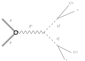
(a) $Z$ channel

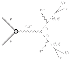
(b) $\gamma,Z$ channels

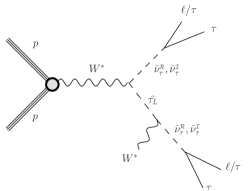
(c) $W$ channel

Figure 1: Decay channels into two $\tau\,\ell/\tau$, from a pair production at the LHC of scalar and pseudoscalar tau left sneutrinos co-LSPs. Decay channels into one $\tau\,\ell/\tau$ plus neutrinos are the same but substituting in (a), (b) and (c) one of the two vertices by a two-neutrino vertex.

The direct production of $\widetilde{\nu}_{\tau}$ occurs via a $Z$ channel giving rise to a pair of scalar and pseudoscalar left sneutrinos, as shown in Fig. 1(a). Note that they are co-LSPs since they have essentially degenerate masses, as explained in the previous section. On the other hand, since the left stau is typically the NLSP its direct production and decay is another important source of the $\widetilde{\nu}_{\tau}$ LSP. In particular, pair production can be obtained through a $\gamma$ or $Z$ decaying into two staus, as shown in Fig. 1(b), with the latter having a dominant RPC prompt decay into a (scalar or pseudoscalar) sneutrino plus an off-shell $W$ producing a soft meson or a pair of a charged lepton and a neutrino. Note that although RPV decays of the stau are possible, e.g. stau into a tau plus a neutrino, they are extremely supressed compared to the RPC one. Numerically, the stau has partial decay widths through RPV diagrams $\sim 10^{-14}-10^{-13}$ GeV, while the ones corresponding to the RPC three-body decays are $\sim 10^{-7}$ GeV. Therefore, its proper decay length is $\sim 10^{-9}$ m, with the BRs corresponding to the RPV decays $<10^{-6}$. Sneutrinos can also be pair produced through a $W$ decaying into a stau and a (scalar or pseudoscalar) sneutrino as shown in Fig. 1(c), with the stau decaying as before.

Subsequently, the pair-produced $\widetilde{\nu}_{\tau}$ can decay into $\tau\,\ell/\tau$. As a result of the mixing between left sneutrinos and Higgses, the sizable decay of $\widetilde{\nu}_{\tau}$ into $\tau\tau$ is possible because of the large value of the tau Yukawa coupling. Other sizable decays into $\tau\,\ell/\tau$ can occur through the Yukawa interaction of $\widetilde{\nu}_{\tau}$ with $\tau$ and charged Higgsinos, via the mixing between the latter and $\ell$ or $\tau$. To analyze these processes we can write approximate formulas for the partial decay widths of the scalar/pseudoscalar tau left sneutrino. The one into $\tau\tau$ is given by:

$$\Gamma\left(\widetilde{\nu}_{\tau}\rightarrow\tau\tau\right)\approx\frac{m_{\widetilde{\nu}_{\tau}}}{{16\pi}}\left(Y_{\tau}Z^{H/A}_{\widetilde{\nu}_{\tau}H_{d}}-Y_{\nu_{\tau}}\frac{Y_{\tau}}{3\lambda}\right)^{2},$$ (12)

where $Y_{\tau}\equiv Y_{e_{33}}$, and $Z^{H/A}$ is the matrix which diagonalizes the mass matrix for the neutral scalars/pseudoscalars. The latter is determined by the neutrino Yukawas, which are the order parameters of the RPV. The contribution of $\lambda$ in the second term of Eq. (12) is due to the charged Higgsino mass that can be approximated by the value of $\mu=3\lambda\frac{v_{R}}{\sqrt{2}}$. The partial decay width into $\tau\ell$ can then be approximated for both sneutrino states by the second term of Eq. (12) with the substitution $Y_{\nu_{\tau}}\rightarrow Y_{\nu_{\ell}}$:

$$\Gamma\left(\widetilde{\nu}_{\tau}\rightarrow\tau\ell\right)\approx\frac{m_{\widetilde{\nu}_{\tau}}}{{16\pi}}\left(Y_{\nu_{\ell}}\frac{Y_{\tau}}{3\lambda}\right)^{2}.$$ (13)

On the other hand, the gauge interactions of $\widetilde{\nu}_{\tau}$ with neutrinos and binos (winos) can produce a large decay width into neutrinos, via the gauge mixing between these gauginos and neutrinos. This partial decay width can be approximated for scalar and pseudoscalar sneutrinos as

$$\sum_{i}{\Gamma(\widetilde{\nu}_{\tau}\to\nu_{\tau}\nu_{i})}\approx\frac{m_{\widetilde{\nu}_{\tau}}}{16\pi}\sum_{i}{\left|\frac{g^{\prime}}{2}U^{V}_{i4}{-}\frac{g}{2}U^{V}_{i5}\right|^{2}},$$ (14)

where $U^{V}$ is the matrix which diagonalizes the mass matrix for the neutral fermions, and the above entries can be approximated as

$$U^{V}_{i4}\approx\frac{{-}g^{\prime}}{\sqrt{2}M_{1}}\sum_{l}{v_{l}U^{PMNS}_{il}},$$

$$U^{V}_{i5}\approx\frac{g}{\sqrt{2}M_{2}}\sum_{l}{v_{l}U^{PMNS}_{il}}.$$ (15)

Here $U^{PMNS}_{il}$ are the entries of the PMNS matrix, with $i$ and $l$ neutrino physical and flavor indices, respectively. The relevant diagrams for $\widetilde{\nu}_{\tau}$ searches that include this decay mode are the same as in Fig. 1, but substituting one of the $\tau\,\ell/\tau$ vertices by a two-neutrino vertex.

Let us remark that other decay channels of the $\widetilde{\nu}_{\tau}$ can be present and have been taken into account in our numerical computation, but they turn out to be negligible for the sneutrino masses that we are interested in this work.

Given the above results valid for three families of right-handed neutrino superfields, we can now follow the prescription of Ref. [10] for improving and recasting the ATLAS search [29] to the case of the $\widetilde{\nu}_{\tau}$. One of the problems with the existing searches [29, 41, 42, 43] is that they are designed for a generic purpose and therefore not optimized for light metastable particles such as the $\widetilde{\nu}_{\tau}$; we thus proposed in Ref. [10] a strategy of improving these searches by lowering trigger thresholds, relying on a high level trigger that utilizes tracker information. This optimization turned out to be quite feasible and considerably improves the sensitivity of the displaced-vertex searches to long-lived $\widetilde{\nu}_{\tau}$. In particular, in the ATLAS 8-TeV analysis, the events must satisfy the following trigger requirements [29]:

• One muon with $p_{\rm T}>50$ GeV and $|\eta|<1.07$, one electron with $p_{\rm T}>120$ GeV or two electrons with $p_{\rm T}>40$ GeV each,

and off-line selection requirements:

• One pair $e^{+}e^{-}$, $\mu^{+}\mu^{-}$ or $e^{\pm}\mu^{\mp}$ with $p_{\rm T}>10$ GeV and $0.02<|\eta|<2.5$ for each particle.

As shown in Ref. [10], the trigger requirement for electrons is so restrictive that it makes the selection efficiency for the dielectron channel be a few percent level, while for the $\mu^{+}\mu^{-}$ and $e^{\pm}\mu^{\mp}$ channels the efficiency can be a few tens of percent. We can however overcome this difficulty by optimizing the trigger requirements for left sneutrino searches by relaxing the momentum thresholds [10]. In fact, it is possible to reduce momentum thresholds for triggers by means of established techniques. For instance, the mu24i trigger used in the ATLAS experiment [44] only requires $p_{\rm T}>24$ GeV; such a low threshold can be achieved thanks to the information from the inner detector. This information can also improve the trigger performance in a wider range of the pseudorapidity of tracks, and thus we can also relax the requirement on $\eta$; from $|\eta|<1.07$ to $|\eta|<2.5$ [44]. It is then argued in Ref. [10] that we can still consider the number of background events to be zero even after we relax the momentum threshold. Consequently, to exploit this trigger instead of that used in Ref. [29] can significantly enhance the sensitivity to light sneutrinos, since the typical momentum of muons from the sneutrino decays is a few tens of GeV. After all, one can use the following criteria for the optimized 8-TeV analysis:

• At least one muon with $p_{\rm T}>24$ GeV.

• One pair $\mu^{+}\mu^{-}$ or $e^{\pm}\mu^{\mp}$ with $p_{\rm T}>10$ GeV and $0.02<|\eta|<2.5$ for each particle.

We can also assume an optimization of the trigger requirements in the 13-TeV searches. It is again discussed in Ref. [10] that one can use the following criteria for the 13-TeV analysis:

• At least one electron or muon with $p_{\rm T}>26$ GeV.

• One pair $\mu^{+}\mu^{-}$, $e^{+}e^{-}$, or $e^{\pm}\mu^{\mp}$ with $p_{\rm T}>10$ GeV and $0.02<|\eta|<2.5$ for each particle.

Since we do not have the 13-TeV result for dilepton displaced-vertex searches for the moment, we just assume the expected number of background events to be zero, which should be validated in the future experiments. It is worth noticing that unlike the previous two trigger requirements, in this case the $p_{T}$ threshold of 26 GeV is for both muons and electrons. The improvement of the selection efficiencies, $\epsilon_{\rm sel}$, for different masses, for the three production processes, and for the $\mu\mu$, $\mu e$, and $ee$ channels, can be found in Tables III-IX of Ref. [10]. As pointed out also in that work, this possible improvement is not only for the ATLAS analysis but also for the CMS one [41].

We can now discuss how to obtain the limits for light sneutrinos. Throughout our analysis, we assume that the number of both background and signal events to be zero, as in the ATLAS 8-TeV search result [44]. The limits from the ATLAS search can be translated into a vertex-level efficiency, taking into account the lack of observation of events for any value of the decay length. Therefore, $\epsilon_{\text{vert}}(c\tau)$ can be obtained as the ratio of the number of signal events compatible with zero observed events (which in this case is 3 as we assume zero background) and that corresponding to the upper limits given in Ref. [29] with an appropriate modification described in Ref. [10]; for example, we can use the purple-shaded solid line of Fig. 3 in the later work to obtain the vertex-level efficiency $\epsilon^{\mu\mu}_{\text{vert}}(c\tau)$ for the dimuon channel. It is found that the efficiency decreases significantly for $c\tau\lesssim 1$ mm, which has important implications for the prospects of the $\widetilde{\nu}_{\tau}$ searches as we will see below. By multiplying the number of the events passing the trigger and event selection criteria with this vertex-level efficiency, we can estimate the total number of signal events; for the 8-TeV case, this is given for the $\mu\mu$ channel by

$${\#}\text{Dimuons} = \left[\sigma(pp\to Z\to\widetilde{\nu}_{\tau}\widetilde{\nu}_{\tau})\epsilon_{\text{sel}}^{Z}+\sigma(pp\to W\to\widetilde{\nu}_{\tau}\widetilde{\tau})\epsilon_{\rm sel}^{W}+\sigma(pp\to\gamma,Z\to\widetilde{\tau}\widetilde{\tau})\epsilon_{\text{sel}}^{\gamma,Z}\right]$$ (16)

$$\times \mathcal{L}\times\left[\text{BR}(\widetilde{\nu}_{\tau}^{\mathcal{R}}\to\mu\mu)\ \epsilon^{\mu\mu}_{\text{vert}}(c\tau^{\mathcal{R}})+\text{BR}(\widetilde{\nu}_{\tau}^{\mathcal{I}}\to\mu\mu)\ \epsilon^{\mu\mu}_{\text{vert}}(c\tau^{\mathcal{I}})\right],$$

where

$$\text{BR}(\widetilde{\nu}_{\tau}\to\mu\mu)\equiv\text{BR}(\widetilde{\nu}_{\tau}\to\tau\mu)\times 0.1739+\text{BR}(\widetilde{\nu}_{\tau}\to\tau\tau)\times(0.1739)^{2}\,,$$ (17)

with 0.1739 the BR of the $\tau$ decay into muons (plus neutrinos), and we use an integrated luminosity of $\mathcal{L}=20.3$ fb^-1 [29] (300 fb^-1 when studying the 13-TeV prospects). The same formula can be applied for the other two channels. If the predicted number of signal events is above 3 the corresponding parameter point of the model is excluded so that this is compatible with zero number of events.

Let us finally remark that in our analysis below, we scan the parameter space of the model and therefore $m_{\widetilde{\nu}_{\tau}}$ can be regarded as a continuous variable, unlike Ref [10] where the sneutrino masses used were 50, 60, 80 and 100 GeV. For the selection efficiency we used a polynomial fitting from the discrete values of $\epsilon_{\rm sel}$ given in Ref. [10] for each production mode, whereas for the vertex-level efficiency, the fitting function is of the form $e^{P[\log(c\tau)]}$, where $P[x]$ is a polynomial in the variable $x$.

4 Strategy for the scanning

In this section we describe the methodology that we employed to search for points of our parameter space that are compatible with the current experimental data on neutrino and Higgs physics, as well as ensuring that the $\widetilde{\nu}_{\tau}$ is the LSP with a mass in the range of $45-100$ GeV. In addition, we demanded the compatibility with some flavor observables. To this end, we performed scans on the parameter space of the model, with the input parameters optimally chosen.

4.1 Sampling the $\mu\nu{\rm SSM}$

For the sampling of the $\mu\nu{\rm SSM}$, we used a likelihood data-driven method employing the Multinest [45] algorithm as optimizer. The goal is to find regions of the parameter space of the $\mu\nu{\rm SSM}$ that are compatible with a given experimental data.

For it we have constructed the joint likelihood function:

$$\mathcal{L}_{\text{tot}}=\mathcal{L}_{\widetilde{\nu}_{\tau}}\times\mathcal{L}_{\text{neutrino}}\times\mathcal{L}_{\text{Higgs}}\times\mathcal{L}_{\text{B physics}}\times\mathcal{L}_{\mu\text{ decay}}\times\mathcal{L}_{m_{\widetilde{\chi}^{\pm}}},$$ (18)

where $\mathcal{L}_{\widetilde{\nu}_{\tau}}$ is basically the prior we impose on the tau left sneutrino mass, $\mathcal{L}_{\text{neutrino}}$ represents measurements of neutrino observables, $\mathcal{L}_{\text{Higgs}}$ Higgs observables, $\mathcal{L}_{\text{B physics}}$ B-physics constraints, $\mathcal{L}_{\mu\text{ decay}}$ $\mu$ decays constraints and $\mathcal{L}_{m_{\widetilde{\chi}^{\pm}}}$ LEPII constraints on the chargino mass.

To compute the spectrum and the observables we used SARAH [46] to generate a SPheno [47, 48] version for the model. We condition that each point is required not to have tachyonic eigenstates. For the points that pass this constraint, we compute the likelihood associated to each experimental data set and for each sample all the likelihoods are collected in the joint likelihood $\mathcal{L}_{\text{tot}}$ (see Eq. (18) above).

4.2 Likelihoods

We used three types of likelihood functions in our analysis. For observables in which a measure is available we use a Gaussian likelihood function defined as follows

$$\mathcal{L}(x)=\exp\left[-\frac{(x-x_{0})^{2}}{2\sigma_{T}^{2}}\right],$$ (19)

where $x_{0}$ is the experimental best fit set on the parameter $x$, $\sigma_{T}^{2}=\sigma^{2}+\tau^{2}$ with $\sigma$ and $\tau$ being respectively the experimental and theoretical uncertainties on the observable $x$.

On the other hand, for any observable for which the constraint is set as lower or upper limit, an example is the chargino mass lower bound, the likelihood function is defined as

$$\mathcal{L}(x) = \frac{\sigma}{\sigma_{T}}\left[1-K\left(D(x)\right)\right]\exp\left[-\frac{(x-x_{0})^{2}p}{2\sigma_{T}^{2}}\right]+\frac{1}{\tau}K\left((x-x_{0})p\right),$$ (20)

where

$$D(x)=\frac{\sigma}{\tau}\left(\frac{(x_{0}-x)p}{\sigma_{T}}\right),\;K(a)=\frac{1}{2}\text{erfc}\bigg{(}\frac{a}{\sqrt{2}}\bigg{)}.$$ (21)

The variable $p$ takes $+1$ when $x_{0}$ represents the lower limit and $-1$ in the case of upper limit, while erfc is the complementary error function.

The last class of likelihood function we used is a step function in such a way that the likelihood is one/zero if the constraint is satisfied/non-satisfied.

It is important to mention that in this work unless explicitly mentioned, the theoretical uncertainties $\tau$ are unknown and therefore are taken to be zero. Subsequently, we present each constraint used in this work together with the corresponding type of likelihood function.

Tau left sneutrino mass

In order to concentrate the sampling in the area in which the mass of the tau left sneutrino $m_{\widetilde{\nu}_{\tau}}\in(45,100)$ GeV, we constructed a likelihood function $\mathcal{L}_{\widetilde{\nu}_{\tau}}$ which is a Gaussian (see Eq. (19)) with mean value $\mu_{m_{\widetilde{\nu}_{\tau}}}=70$ GeV and width $\sigma_{m_{\widetilde{\nu}_{\tau}}}=10$ GeV, and included it in the combined likelihood.

Neutrino observables

We used the results for NO from Ref. [32] summarized in Table 1, where $\delta m^{2}=m_{2}^{2}-m_{1}^{2}$ and $\Delta m^{2}=m_{3}^{2}-(m_{2}^{2}+m_{1}^{2})/2$.

Parameters	$\sin^{2}{\theta_{12}}$	$\sin^{2}{\theta_{13}}$	$\sin^{2}{\theta_{23}}$	$\delta m^{2}\,/\,10^{-5}$ (eV2)	$\Delta m^{2}\,/\,10^{-3}$ (eV2)
$\mu_{exp}$	$0.297$	$0.0215$	$0.425$	$7.37$	$2.525$
$\sigma_{exp}$	$0.017$	$0.0007$	$0.021$	$0.17$	$0.042$

Table 1: Neutrino data used in the sampling of the $\mu\nu$SSM.

For each of the observables listed in the neutrino sector, the likelihood function is a Gaussian (see Eq. (19)) centered at the mean value $\mu_{exp}$ and with width $\sigma_{exp}$. Concerning the cosmological upper bound on the sum of the masses of the light active neutrinos given by $\sum m_{\nu_{i}}<0.12$ eV [49], even though we did not include it directly in the total likelihood, we imposed it on the viable points obtained.

Higgs observables

Before the discovery of the SM-like Higgs boson, the negative searches of Higgs signals at the Tevatron, LEP and LHC, were transformed into exclusions limits that must be used to constrain any model. Its discovery at the LHC added crucial constraints that must be taken into account in those exclusion limits. We have considered all these constraints in the analysis of the $\mu\nu{\rm SSM}$, where the Higgs sector is extended with respect to the MSSM as discussed in Section 2. For constraining the predictions in that sector of the model, we interfaced HiggsBounds v5.3.2 [50, 51] with MultiNest. First, several theoretical predictions in the Higgs sector (using a $\pm 3$ GeV theoretical uncertainty on the SM-like Higgs boson) are provided to determine which process has the highest exclusion power, according to the list of expected limits from LEP and Tevatron. Once the process with the highest statistical sensitivity is identified, the predicted production cross section of scalars and pseudoscalars multiplied by the BRs are compared with the limits set by these experiments. Then, whether the corresponding point of the parameter under consideration is allowed or not at 95% confidence level is indicated. In constructing the likelihood from HiggsBounds constraints, the likelihood function is taken to be a step function. Namely, it is set to one for points for which Higgs physics is realized, and zero otherwise. Finally, in order to address whether a given Higgs scalar of the $\mu\nu{\rm SSM}$ is in agreement with the signal observed by ATLAS and CMS, we interfaced HiggsSignals v2.2.3 [52, 53] with MultiNest. A $\chi^{2}$ measure is used to quantitatively determine the compatibility of the $\mu\nu{\rm SSM}$ prediction with the measured signal strength and mass. The experimental data used are those of the LHC with some complements from Tevatron. The details of the likelihood evaluation can be found in Refs. [52, 53].

B decays

$b\to s\gamma$ is a flavour changing neutral current (FCNC) process, and hence it is forbidden at tree level in the SM. However, its occurs at leading order through loop diagrams. Thus, the effects of new physics (in the loops) on the rate of this process can be constrained by precision measurements. In the combined likelihood, we used the average value of $(3.55\pm 0.24)\times 10^{-4}$ provided in Ref. [54]. Notice that the likelihood function is also a Gaussian (see Eq. (19)). Similarly to the previous process, $B_{s}\to\mu^{+}\mu^{-}$ and $B_{d}\to\mu^{+}\mu^{-}$ are also forbidden at tree level in the SM but occur radiatively. In the likelihood for these observables (19), we used the combined results of LHCb and CMS [55], $\text{BR}(B_{s}\to\mu^{+}\mu^{-})=(2.9\pm 0.7)\times 10^{-9}$ and $\text{BR}(B_{d}\to\mu^{+}\mu^{-})=(3.6\pm 1.6)\times 10^{-10}$. Concerning the theoretical uncertainties for each of these observables we take $\tau=10\%$ of the corresponding best fit value. We denote by $\mathcal{L}_{\text{B physics}}$ the likelihood from $b\to s\gamma$, $B_{s}\to\mu^{+}\mu^{-}$ and $B_{d}\to\mu^{+}\mu^{-}$.

$\mu\to e\gamma$ and $\mu\to eee$

We also included in the joint likelihood the constraint from BR$(\mu\to e\gamma)<5.7\times 10^{-13}$ and BR$(\mu\to eee)<1.0\times 10^{-12}$. For each of these observables we defined the likelihood as a step function. As explained before, if a point is in agreement with the data, the likelihood $\mathcal{L}_{\mu\text{ decay}}$ is set to 1 otherwise to 0.

Let us point out here that we did not try to explain the interesting but not conclusive 3.5$\sigma$ discrepancy between the measurement of the anomalous magnetic moment of the muon and the SM prediction, $\Delta a_{\mu}=a_{\mu}^{\text{exp}}-a_{\mu}^{\text{SM}}=(26.8\pm 6.3\pm 4.3)\times 10^{-10}$ [4]. Since we decouple the rest of the SUSY spectrum with respect to the tau left sneutrino mass, we do not expect a large SUSY contribution over the SM value. We checked for the points fulfilling all constrains discussed in Section 5, that the extra contribution $a_{\mu}^{\text{SUSY}}$ is within the SM uncertainty.

Chargino mass bound

In RPC SUSY, the lower bound on the lightest chargino mass of about $94$ GeV depends on the spectrum of the model [4, 56]. Although in the $\mu\nu{\rm SSM}$ there is RPV and therefore this constraint does not apply automatically, to compute $\mathcal{L}_{m_{\widetilde{\chi}^{\pm}}}$ we have chosen a conservative limit of $m_{\widetilde{\chi}^{\pm}_{1}}>92$ GeV with the theoretical uncertainty $\tau=5\%$ of the chargino mass.

4.3 Input parameters

In order to efficiently scan for the $\widetilde{\nu}_{\tau}$ LSP in the $\mu\nu$SSM with a mass in the range $45-100$ GeV, it is important to identify first the parameters to be used, and optimize their number and their ranges of values. This is what we carry out here, where we discuss the most relevant parameters for obtaining correct neutrino and Higgs physics, providing at the same time the $\widetilde{\nu}_{\tau}$ as the LSP with the mass in the desired range.

The relevant parameters in the neutrino sector of the $\mu\nu{\rm SSM}$ are $\lambda,\kappa,v_{R},v_{i},Y_{\nu_{i}},\tan\beta$ and $M$ (see Eq. (6)). Since $\lambda,\kappa$ and $v_{R}$ are crucial for Higgs physics, we will fix first them to appropriate values. The parameter $\tan\beta$ is also important for both, Higgs and neutrino physics, thus we will consider a narrow range of possible values to ensure good Higgs physics. Concerning $M$, which is a kind of average of bino and wino soft masses (see Eq. (5)), inspired by GUTs we will assume $M_{2}=2M_{1}$, and scan over $M_{2}$. On the other hand, sneutrino masses introduce in addition the parameters $T_{{\nu}_{i}}$ (see Eq. (7)). In particular, $T_{{\nu}_{3}}$ is the most relevant one for our discussion of the $\widetilde{\nu}_{\tau}$ LSP, and we will scan it in an appropriate range of small values. Since the left sneutrinos of the first two generations must be heavier, we will fix $T_{{\nu}_{1,2}}$ to a larger value.

Summarizing, we will perform scans over the 9 parameters $Y_{\nu_{i}},v_{i},T_{{\nu}_{3}},\tan\beta,M_{2}$, as shown in Table 2, using log priors (in logarithmic scale) for all of them, except for $\tan\beta$ which is taken to be a flat prior (in linear scale). The ranges of $v_{i}$ and $Y_{\nu_{i}}$ are natural in the context of the electroweak-scale seesaw of the $\mu\nu{\rm SSM}$. The range of $T_{\nu_{3}}$ is also natural if we follow the usual assumption based on the supergravity framework discussed in Eq. (11) that the trilinear parameters are proportional to the corresponding Yukawa couplings, i.e. in this case $T_{\nu_{3}}=A_{\nu_{3}}Y_{\nu_{3}}$ implying $-A_{\nu_{3}}\in$ ($1,10^{4}$) GeV. Concerning $M_{2}$, its range of values is taken such that a bino at the bottom of the neutralino spectrum leaves room to accommodate a $\widetilde{\nu}_{\tau}$ LSP with a mass below 100 GeV. Scans 1 ($S_{1}$) and 2 ($S_{2}$) correspond to different values of $\tan\beta$, and other benchmark parameters as shown in Table 3.

In Table 3 we choose first two values of $\lambda$, covering a representative region of this parameter. From a small/moderate value, $\lambda\approx 0.1$ ($S_{1}$), to a large value, $\lambda\approx 0.4$ ($S_{2}$), in the border of perturbativity up to the GUT scale [36]. For scan $S_{1}$, since $\lambda$ is small we are in a similar situation as in the MSSM, and moderate/large values of $\tan\beta$, $|T_{u_{3}}|$, and soft stop masses, are necessary to obtain the correct SM-like Higgs mass. In addition, if we want to avoid the chargino mass bound of RPC SUSY, the value of $\lambda$ also force us to choose a moderate/large value of $v_{R}$ to obtain a large enough value of $\mu=3\lambda\frac{v_{R}}{\sqrt{2}}$. In particular, we choose $v_{R}=1750$ GeV giving rise to $\mu\approx 379$ GeV. The latter parameters, $\lambda$ and $v_{R}$, together with $\kappa$ and $T_{\lambda}$ are also relevant to obtain the correct values of the off-diagonal terms of the mass matrix mixing the right sneutrinos with Higgses. As explained in Eq. (10), the parameters $\kappa$ and $v_{R}$ (together with $T_{\kappa}$) are also crucial to determine the mass scale of the right sneutrinos. In scan $S_{1}$, where we choose $T_{\kappa}=-390$ GeV to have heavy pseudoscalar right sneutrinos (of about 1190 GeV), the value of $\kappa$ has to be large enough in order to avoid too light (even tachyonic) scalar right sneutrinos. Choosing $\kappa=0.4$, we get masses for the latter of about $700-755$ GeV.

Scan 1 ($S_{1}$)	Scan 2 ($S_{2}$)
$\tan\beta\in(10,16)$	$\tan\beta\in(1,4)$
$Y_{\nu_{i}}\in(10^{-8},10^{-6})$
$v_{i}\in(10^{-6},10^{-3})$
$-T_{\nu_{3}}\in(10^{-6},10^{-4})$
$M_{2}\in(150,2000)$

Table 2: Range of low-energy values of the input parameters that are varied in the two scans, where $Y_{\nu_{i}}$, $v_{i}$, $T_{\nu_{3}}$ and $M_{2}$ are $\log$ priors while $\tan\beta$ is a flat prior. The VEVs $v_{i}$, and the soft parameters $T_{\nu_{3}}$ and $M_{2}$, are given in GeV.

Parameter	Scan 1 ($S_{1}$)	Scan 2 ($S_{2}$)
$\lambda$	0.102	0.42
$\kappa$	0.4	0.46
$v_{R}$	1750	421
$T_{\lambda}$	340	350
$-T_{\kappa}$	$390$	$108$
$-T_{u_{3}}$	$4140$	$1030$
$m_{\widetilde{Q}_{3L}}$	2950	1972
$m_{\widetilde{u}_{3R}}$	1140	1972
$M_{3}$	2700
$m_{\widetilde{Q}_{1,2L}},m_{\widetilde{u}_{1,2R}},m_{\widetilde{d}_{1,2,3R}},m_{\widetilde{e}_{1,2,3R}}$	1000
$T_{u_{1,2}}$	0
$T_{d_{1,2}}$, $T_{d_{3}}$	0, $100$
$T_{e_{1,2}}$, $T_{e_{3}}$	0, $40$
$-T_{\nu_{1,2}}$	$10^{-3}$

Table 3: Low-energy values of the input parameters that are fixed in the two scans. The VEV $v_{R}$ and the soft trilinear parameters, soft gluino masses and soft scalar masses are given in GeV.

For scan $S_{2}$, where we choose a large value for $\lambda$, we are in a similar situation as in the NMSSM, and a small value of $\tan\beta$, and moderate values of $|T_{u_{3}}|$ and soft stop masses, are sufficient to reproduce the correct SM-like Higgs mass. Now, a moderate value of $v_{R}$ is sufficient to obtain a large enough value of $\mu$. In particular, we choose $v_{R}=421$ GeV giving rise to $\mu\approx 375$ GeV. This value of $v_{R}$ implies that $|T_{\kappa}|$ cannot be as large as for scan $S_{1}$ because then a too large value of $\kappa$ would be needed to avoid tachyonic scalar right sneutrinos. Thus we choose $T_{\kappa}=-108$ GeV, and $\kappa=0.42$, which produces scalar and pseudoscalar sneutrinos lighter than in scan $S_{1}$ but still heavier than $\widetilde{\nu}_{\tau}$ LSP and left stau NLSP. In particular, their masses are in the ranges $225-256$ GeV and $345-355$ GeV, respectively.

The values of the parameters shown below $m_{\widetilde{u}_{3R}}$ in Table 3, concerning gluino, and squark and slepton masses, and quark and lepton trilinear parameters, are not specially relevant for our analysis, and we choose for each of them the same values for both scans. Finally, compared to the values of $T_{\nu_{3}}$, the values chosen for $T_{\nu_{1,2}}$ are natural within our framework $T_{\nu_{1,2}}=A_{\nu_{1,2}}Y_{\nu_{1,2}}$, since larger values of the Yukawa couplings are required for similar values of $A_{\nu_{i}}$. In the same way, the values of $T_{d_{3}}$ and $T_{e_{3}}$ have been chosen taking into account the corresponding Yukawa couplings

5 Results

By using the methods described in the previous sections, we evaluate now the current and potential limits on the parameter space of our scenario from the displaced-vertex searches with the 8-TeV ATLAS result [29], and discuss the prospects for the 13-TeV searches.

To find regions consistent with experimental observations we have performed about 72 million of spectrum evaluations in total and the total amount of computer required for this was approximately 380 CPU years.

To carry this analysis out, we follow several steps. First, we select points from the scan that lie within $\pm 3\sigma$ of all neutrino physics observables, namely the mixing angles and mass squared differences. Second, we put $\pm 3\sigma$ cuts from $b\to s\gamma$, $B_{s}\to\mu^{+}\mu^{-}$ and $B_{d}\to\mu^{+}\mu^{-}$. The points that pass these cuts are required to satisfy also the upper limits of $\mu\to e\gamma$ and $\mu\to eee$. The third step in the selection of our points is to ensure a tau left sneutrino LSP with $m_{\widetilde{\nu}_{\tau}}\in(45,{100})$ GeV, and the left stau as the NLSP. In the fourth step we impose that Higgs physics is realized. As already mentioned, we use HiggsBounds and HiggsSignals taking into account the constraints from the latest 13-TeV results. In particular, we require that the p-value reported by HiggsSignals be larger than 5 %. It is worth noticing here that, with the help of Vevacious [57], we have also checked that the EWSB vacua corresponding to the previous allowed points are stable.

The final set of cuts is related to $\widetilde{\nu}_{\tau}$ LSP searches with displaced vertices. From the points left above, we select those with decay length $c\tau>0.1$ mm in order to be constrained by the current experimental results, as mentioned in previous sections. Finally, since the number of signal events compatible with zero observed events is 3, we look for points with a number of signal events above 3.

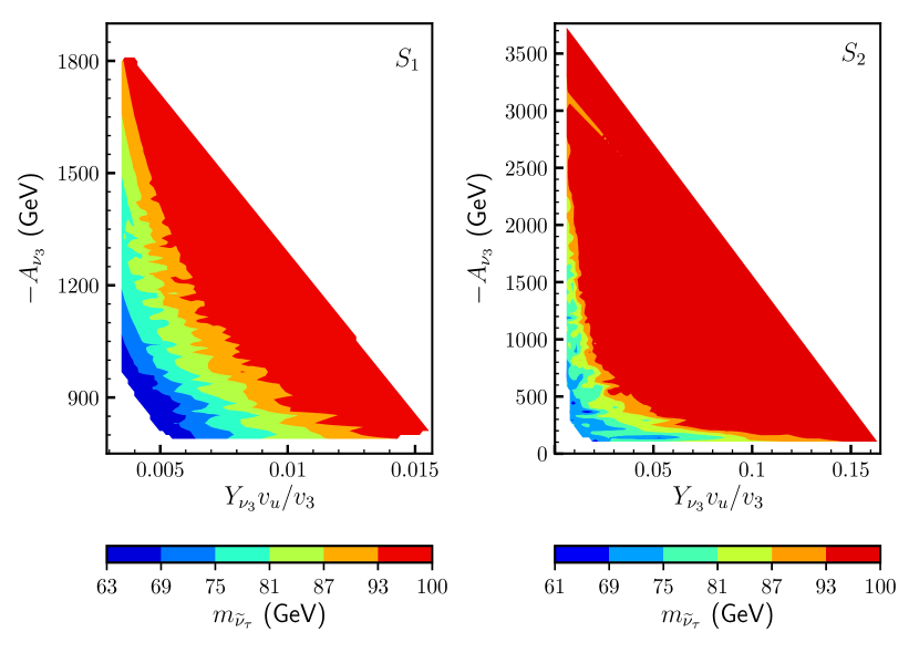
Figure 2: $-A_{\nu_{3}}$ versus $Y_{\nu_{3}}v_{u}/{v_{3}}$ for scan $S_{1}$ (left) and scan $S_{2}$ (right). The colours indicate different values of the tau left sneutrino LSP mass.

5.1 Constraints from neutrino/sneutrino physics.

As discussed in detail in Section 2, reproducing neutrino physics is an important asset of the $\mu\nu{\rm SSM}$. It is therefore important to analyze first the constraints imposed by this requirement on the relevant parameter space of the model when the $\widetilde{\nu}_{\tau}$ is the LSP.

Imposing all the cuts discussed above, with the exception of the one associated to the number of signal events, we show in Fig. 2 the values of the parameter $A_{\nu_{3}}$ versus the prefactor in Eq. (11), $Y_{\nu_{3}}v_{u}/{v_{3}}$, giving rise to a mass of the $\widetilde{\nu}_{\tau}$ in the desired range $45-100$ GeV. The colours indicate different values of this mass. Scan $S_{1}$ ($S_{2}$) is shown in the left (right)-hand side of the figure. Let us remark that these plots have been obtained using the full numerical computation including loop corrections, although the tree-level mass in Eq. (11) gives a good qualitative idea of the results. In particular, in scan $S_{1}$ we can see that the allowed range of $-A_{\nu_{3}}$ is $779-1820$ GeV, corresponding to $-T_{\nu_{3}}$ in the range $8.3\times 10^{-6}-3.5\times 10^{-5}$ GeV. We can also see, as can be deduced from Eq. (11), that for a fixed value of $-A_{\nu_{3}}$ ($Y_{\nu_{3}}v_{u}/{v_{3}}$) the greater $Y_{\nu_{3}}v_{u}/{v_{3}}$ ($-A_{\nu_{3}}$) is, the greater $m_{\widetilde{\nu}_{\tau}}$ becomes. For scan $S_{2}$, the allowed range of $-A_{\nu_{3}}$ turns out to be $67-3764$ GeV, corresponding to $-T_{\nu_{3}}$ in the range $2.1\times 10^{-6}-4.9\times 10^{-5}$ GeV. The differences in the range of allowed values for $A_{\nu_{3}}$ and $Y_{\nu_{3}}v_{u}/{v_{3}}$ of the scan $S_{1}$ with respect to $S_{2}$, are due to the negative vs. the positive contribution of the sum of the second and third terms in the bracket of Eq. (11), respectively, as well as to the different values of $v_{R}$ which appears also as a prefactor in that equation.

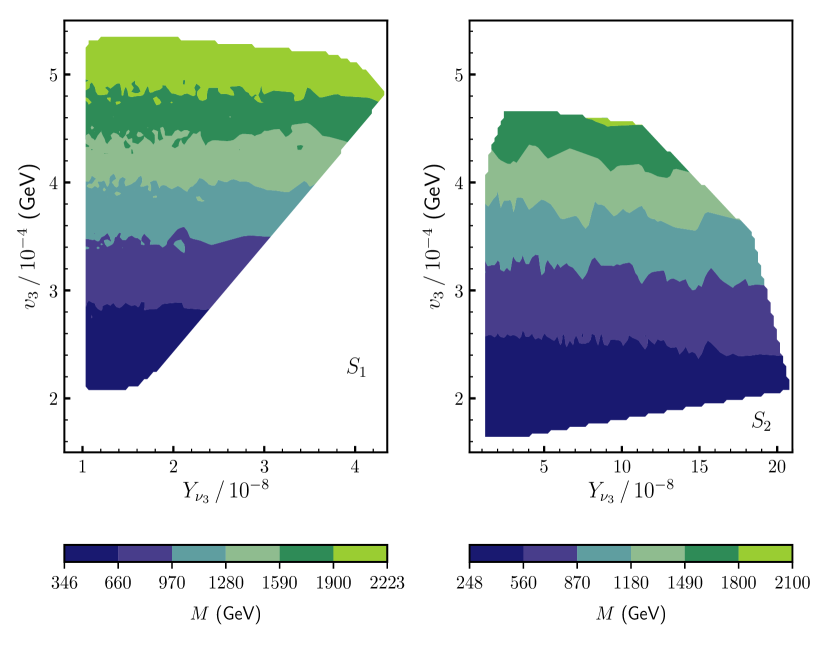
Figure 3: $v_{3}$ versus $Y_{\nu_{3}}$ for scan $S_{1}$ (left) and scan $S_{2}$ (right). The colours indicate different values of the gaugino mass parameter $M$ defined in Eq. (5).

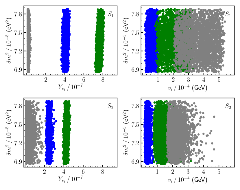
Figure 4: $\delta m^{2}$ versus neutrino Yukawas (left) and left sneutrino VEVs (right) for scan $S_{1}$ (top) and $S_{2}$ (bottom). Colors blue, green and grey correspond to $i=1,2,3$, respectively.

Let us finally note that $m_{\widetilde{\nu}_{\tau}}$ is always larger than about 61 GeV, which corresponds to half of the mass of the SM-like Higgs (remember that we allow a $\pm$3 GeV theoretical uncertainty on its mass). For smaller masses, the latter would dominantly decay into sneutrino pairs, leading to an inconsistency with Higgs data.

In Fig. 3, we show $v_{3}$ vs. $Y_{\nu_{3}}$ for scan $S_{1}$ (left) and scan $S_{2}$ (right), with the colours indicating now different values of $M$. There we can see that the greater $v_{3}$ is, the greater $M$ becomes. In addition, for a fixed value of $v_{3}$, $M$ is quite independent of the variation in $Y_{\nu_{3}}$. This confirms that, as explained in solution 2) of Subsection 2.1, the gaugino seesaw is the dominant one for the third neutrino family. From the figure, we can see that the range of $M$ reproducing the correct neutrino physics is $346-2223$ GeV for scan $S_{1}$ and $248-2100$ GeV for $S_{2}$, corresponding to $M_{2}$ in the range $236-1515$ GeV and $169-1431$ GeV, respectively. Note that for a fixed value of $v_{3}$, when $Y_{\nu_{3}}$ is sufficiently large the $\widetilde{\nu}_{\tau}$ becomes heavier than 100 GeV, and these points are not shown in the figure. As can also be seen, $Y_{\nu_{3}}$ acquires larger values in scan $S_{2}$ than in $S_{1}$, in agreement with the discussion of Fig. 2.

The values of $Y_{\nu_{3}}$ and $v_{3}$ used in order to obtain a $\widetilde{\nu}_{\tau}$ LSP in turn constrain the values of $Y_{\nu_{1,2}}$ and $v_{1,2}$ producing a correct neutrino physics. This is shown in Fig. 4, where $\delta m^{2}$ vs. $Y_{\nu_{i}}$ and $v_{i}$ is plotted. As we can see, we obtain the hierarchy qualitatively discussed in solution 2) of Subsection 2.1, i.e. $Y_{\nu_{3}}<Y_{\nu_{1}}<Y_{\nu_{2}}$, and $v_{1}<v_{2}\raise 1.29167pt\hbox{$\;<$\kern-7.5pt\raise-4.73611pt\hbox{$\sim\;$}}v_{3}$. The values of the Yukawas $Y_{\nu_{1,2}}$ in scan $S_{2}$ are smaller than the corresponding ones in $S_{1}$ because for these two families the $\nu_{R}$-Higgsino seesaw contributes significantly to the neutrino masses, and $v_{R}$ is smaller for scan $S_{2}$. Concerning the absolute value of neutrino masses, we obtain $m_{\nu_{1}}\sim$ 0.002 eV, $m_{\nu_{2}}\sim$ 0.008 eV, and $m_{\nu_{3}}\sim$ 0.05 eV, fulfilling the cosmological upper bound on the sum of neutrino masses of $0.12$ eV mentioned in Subsection 4.3. The predicted value of the sum of the neutrino masses can be tested in future CMB experiments such as CMB-S4 [58]. It is also worth noticing here that these hierarchies of neutrino Yukawas and left sneutrino VEVS, give rise to a $\widetilde{\nu}_{\mu}$ mass in the range $766-1568$ GeV for scan $S_{1}$ and $466-945$ GeV for $S_{2}$, producing the contributions $a_{\mu}^{\text{SUSY}}\sim 3\times 10^{-10}$ and $\sim 1\times 10^{-10}$, respectively, which are within the SM uncertainty of the muon anomalous magnetic moment as mentioned in Subsection 4.2.

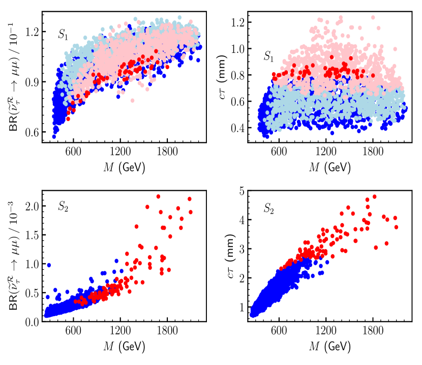
Figure 5: (Left) Branching ratio versus $M$ for the decay of a scalar $\widetilde{\nu}_{\tau}$ LSP with $m_{\widetilde{\nu}_{\tau}}\in(61-100)$ GeV into $\mu\mu$ for scan $S_{1}$ (top) and $S_{2}$ (bottom). (Right) Proper decay length $c\tau$ of the scalar $\widetilde{\nu}_{\tau}$ LSP versus $M$ for scan $S_{1}$ (top) and $S_{2}$ (bottom). In all plots, the dark-red points indicate that the number of signal events is above 3 analyzing the prospects for the 13-TeV search with an integrated luminosity of 300 fb^-1, combining the $\mu\mu$, $e\mu$ and $ee$ channels, and considering also the optimization of the trigger requirements discussed in the text. The light-red points in scan $S_{1}$ although have a number of signal events above 3, are already excluded by the LEP result, as discussed in the text. The dark-blue points indicate that the number of signal events is below 3 and therefore inaccessible. The light-blue points in scan $S_{1}$ have also a number of signal events below 3, and, in addition, are already excluded by the LEP result.

5.2 Constraints from accelerator searches

Once the neutrino (and sneutrino) physics has determined the relevant regions of the parameter space of the $\widetilde{\nu}_{\tau}$ LSP in the $\mu\nu{\rm SSM}$, we are ready to analyze the reach of the LHC search.

Given that for each scan the largest neutrino Yukawa is $Y_{\nu_{2}}$, the most important contribution to the dilepton BRs comes from the channel $\widetilde{\nu}_{\tau}\rightarrow\tau\mu$. We also expect that the BR($\widetilde{\nu}_{\tau}\to\mu\mu$) is larger for scan $S_{1}$ than for $S_{2}$, as can be checked in Fig. 5 (left plots), where BR($\widetilde{\nu}^{\mathcal{R}}_{\tau}\to\mu\mu$) is plotted vs. $M$, for the points fulfilling all constraints from neutrino/sneutrino physics (although not shown here, a similar figure is obtained in the case of the pseudoscalar $\widetilde{\nu}^{\mathcal{I}}_{\tau}$). The main reason is the smaller (larger) value of $\lambda$ ($\tan\beta$) for scan $S_{1}$ with respect to $S_{2}$, which are crucial parameters in Eq. (13) for the partial decay width. Although $\tan\beta$ does not appear explicitly in that equation, note that $Y_{\tau}=({\sqrt{2}m_{\tau}}/{v})\sqrt{\tan^{2}\beta+1}$. In addition, as shown in Fig. 4, the value of $Y_{\nu_{2}}$ is larger for scan $S_{1}$ than for $S_{2}$, contributing therefore to larger BRs. We can also observe in both plots of Fig. 5 for the BRs that they increase with larger values of $M$. This can be understood from Eq. (14) showing that larger values of $M$ decrease the decay width to neutrinos. In Fig. 5 (right plots), we show the proper decay length of the $\widetilde{\nu}^{\mathcal{R}}_{\tau}$ vs. $M$. Clearly, this is larger for scan $S_{2}$ than for $S_{1}$ because the BRs into charged leptons are smaller in the former case, as discussed before. Let us finally remember that the lower and upper bounds on $M$ in the figure, have their origin in the analysis of the previous section reproducing neutrino (sneutrino) physics.

It is apparent that in scan $S_{2}$ for $M$ larger than about 1000 GeV, the points that we find fulfilling all constraints are not uniformly distributed. This happens essentially because the value of $v_{R}$ is smaller than in scan $S_{1}$ modifying the relevant contribution of the $\nu_{R}$-Higgsino seesaw for the first two families, in such a way that is more difficult to reproduce neutrino physics unless more accurate values of the neutrino Yukawas are input in the computation. As obtained in Subsection 5.1, and can be seen in Fig. 4, the allowed values of $Y_{\nu_{3}}$ are larger for $S_{2}$. This makes more complicated to obtain the correct mixing, producing a tuning in the parameters. To obtain these more accurate values, we would have had to run Multinest a much longer time making the task very computer resources demanding. This is not really necessary since it is not going to affect the shape of the figure, and therefore neither the conclusions obtained. In addition, let us point out that we could have also modified the values of the parameters used for scan $S_{2}$ reproducing more easily neutrino physics, e.g. increasing $v_{R}$ and modifying accordingly the other parameters to keep the good Higgs physics.

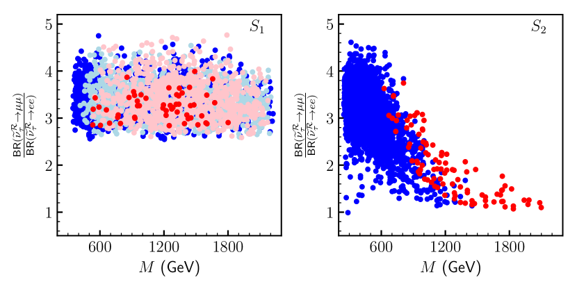
Figure 6: Ratios of the branching fractions of $\widetilde{\nu_{\tau}}\to\mu\mu$ and $\widetilde{\nu_{\tau}}\to ee$ for scan $S_{1}$ (left) and scan $S_{2}$ (right). The color code is the same as in Fig. 5.

In all plots of Fig 5, the (light- and dark-)red points correspond to regions of the parameter space where the number of signal events is above 3. Note that this only occurs for the 13-TeV analysis with an integrated luminosity of $\mathcal{L}=300$ fb^-1. For the 8-TeV analysis, even considering the optimization of the trigger requirements, no points have a number of signal events larger than 3. However, we have checked that the light-red points in scan $S_{1}$ are already excluded by the LEP bound on left sneutrino masses [20, 21, 22, 23, 24, 25]. To carry out this analysis, one can consider e.g. Fig. 6a of Ref. [23], where the cross section upper limit for tau sneutrinos decaying directly to $\ell\ell\tau\tau$ via a dominant $\hat{L}\hat{L}\hat{e}^{c}$ operator is shown. Assuming ${\rm BR}=1$, a lower bound on the sneutrino mass was obtained through the comparison with the MSSM cross section for pair production of tau sneutrinos. To recast this result we multiplied this cross section by the factor $\text{BR}(\widetilde{\nu}_{\tau}^{\mathcal{R}}\to\tau\mu)\times\text{BR}(\widetilde{\nu}_{\tau}^{\mathcal{I}}\to\tau\mu)$ for each of our points. For an average value of $\text{BR}(\widetilde{\nu}_{\tau}\to\mu\mu)=0.1$ as we can see in Fig 5, the cross section must be multiplied then by a factor of $\sim 0.33$, lowering the bound on the sneutrino mass from about 90 GeV in the case of trilinear RPV to about 74 GeV in our case (see Fig. 7 below). This result turns out to be qualitatively different from the one of Ref. [10], where no bound on the sneutrino mass was obtained from recasting the LEP result. This is due to the simplified assumption made in that work that all neutrino Yukawas have the same value and therefore democratic BRs, implying a smaller value for the above factor. On the other hand, using Table II of Ref. [10] with the BRs modified appropriately, we have checked that the lack of constraint on the sneutrino mass from the production of a pair of left staus at LEP obtained in that work, is still valid. We have arrived at the same conclusion for LEP mono-photon search and LHC mono-photon and mono-jet searches, taking also into account the most recent results [59, 60]. Let us finally remark that the (light- and dark-)blue points correspond to regions where the number of signal events is below 3, and therefore inaccessible. In addition, we have checked that the light-blue points on top of the dark-blue ones are already excluded by the LEP result.

Concerning scan $S_{2}$, we can see in Fig 5 that the BRs into charged leptons are about two orders of magnitude smaller than for $S_{1}$, and therefore following the above discussion we have checked that no points are excluded by LEP results in this case. Note that although these BRs are smaller, still a significant number of points with signal events above 3 can be obtained when $M$ increases because of the larger value of the decay length, which gives rise to a larger vertex-level efficiency.

Figure 5 also shows that the sensitivity of the dilepton displaced-vertex searches to $\widetilde{\nu}_{\tau}$ is limited by their small efficiency for $c\tau\lesssim 1$ mm, especially for the $S_{1}$ case. It is, however, worth noticing that we may even probe such a short lifetime region by optimizing the search strategy for the sub-millimeter displaced vertices, as discussed in Refs. [61, 62]. Our result highly motivates a dedicated work for such an optimization, which we defer to another occasion.

As discussed in Section 3, the value of $Y_{\nu_{1}}$ is rather large in our scenario, and therefore we expect a sizable branching fraction for the $\widetilde{\nu}_{\tau}\to ee$ channel. In fact, the ratio of the branching fractions for the $\widetilde{\nu}_{\tau}\to ee$ and $\widetilde{\nu}_{\tau}\to\mu\mu$ channels has important implications for our scenario since it reflects the information from the neutrino data via the neutrino Yukawa couplings (see Fig. 4). To see this, we plot it against the parameter $M$ in Fig. 6. It is found that for the $S_{1}$ case, the ratios $R_{\mu/e}\equiv{\rm BR}(\widetilde{\nu}^{\cal R}_{\tau}\to\mu\mu)/{\rm BR}(\widetilde{\nu}^{\cal R}_{\tau}\to ee)$ are in the range $3\lesssim R_{\mu/e}\lesssim 5$, while for the $S_{2}$ case they are more widely distributed: $1\lesssim R_{\mu/e}\lesssim 4.6$. This different behaviour can be understood if we realize that for scan $S_{1}$ the second term of $\text{BR}(\widetilde{\nu}_{\tau}\to\mu\mu)$ in Eq. (17) is negligible with respect to the first one, and the same for the corresponding terms of $\text{BR}(\widetilde{\nu}_{\tau}\to ee)$. Thus, with the approximation in Eq. (13) one gets $R_{\mu/e}\approx(Y_{\nu_{\mu}}/Y_{\nu_{e}})^{2}$, which using the results for the neutrino Yukawas in Fig. 4 gives rise to the above range around 3.5. However, for scan $S_{2}$ the term of $\text{BR}(\widetilde{\nu}_{\tau}\to ee)$ proportional to $\text{BR}(\widetilde{\nu}_{\tau}\to\tau\tau)$ is not negligible with respect to the one proportional to $\text{BR}(\widetilde{\nu}_{\tau}\to\tau e)$, which is much smaller than in scan $S_{1}$, due to the contribution of the first term in Eq. (12). This implies that the ratio $R_{\mu/e}$ in scan $S_{2}$ can be smaller than in $S_{1}$, as can be seen in the figure. Now, if we particularly focus on the parameter points that can be probed at the 13-TeV LHC, the $S_{2}$ case predicts $R_{\mu/e}\lesssim 3.6$, and thus we can in principle distinguish this case from the $S_{1}$ case by measuring this ratio in the future LHC experiments such as the high-luminosity LHC.

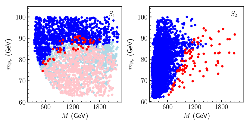
Figure 7: Tau left sneutrino LSP mass versus $M$ for scan $S_{1}$ (left) and scan $S_{2}$ (right). The color code is the same as in Fig. 5.

Finally, we show in Fig. 7 $m_{\widetilde{\nu}_{\tau}}$ vs. $M$. For scan $S_{1}$ (left plot), tau left sneutrino masses in the range $74-91$ GeV can be probed, corresponding to a gaugino mass parameter $M$ in the range $532-1801$ GeV, i.e. $M_{2}\in(363-1228)$ GeV. Clearly, red points appear in these regions because smaller sneutrino masses produce larger decay lengths. Since decay lengths are larger for scan $S_{2}$, the range of sneutrino masses that can be probed is also larger than for $S_{1}$. In particular, we can see in the right plot that the range of sneutrino masses is $63-95$ GeV. In this scenario, $M$ is in the range $625-2100$ GeV, correspoding to $M_{2}\in(427-1431)$ GeV. Let us finally mention that points with sneutrino masses slightly larger than 100 GeV, and with $c\tau>0.1$ mm, exist, but since they are not constrained by the number of signals events and therefore cannot be probed at the LHC run 3, we do not show them in the figures. In any cases, if we actually detect the $\widetilde{\nu}_{\tau}$ signal and measure its mass and lifetime in future experiments, we can considerably narrow down the allowed parameter region, which plays an important role in testing the $\mu\nu{\rm SSM}$.

6 Conclusions

In the framework of the $\mu\nu{\rm SSM}$, where there is RPV and the several decay BRs of the LSP significantly decrease the signals, there is a lack of experimental bounds on the masses of the sparticles. To fill this gap in SUSY searches, it is then crucial to analyze the recent experimental results that can lead to limits on sparticle masses in this model, and the prospects for the searches with a higher energy and luminosity.

With this purpose, we recast the result of the ATLAS 8-TeV displaced dilepton search from long-lived particles [29], to obtain the potential limits on the parameter space of the tau left sneutrino LSP in the $\mu\nu{\rm SSM}$ with a mass in the range $45-100$ GeV. A crucial point of the analysis, which differentiates the $\mu\nu{\rm SSM}$ from other SUSY models is that neutrino masses and mixing angles are predicted by the generalized electroweak scale seesaw of the $\mu\nu{\rm SSM}$ once the parameters of the model are fixed. This is obtained at tree level when three generations of right-handed neutrinos are considered. Therefore, the sneutrino couplings have to be chosen so that the neutrino oscillation data are reproduced, which has important implications for the sneutrino decay properties.

The sneutrino LSP is produced via the $Z$-boson mediated Drell-Yan process or through the $W$- and $\gamma/Z$-mediated process accompanied with the production and decay of the left stau NLSP. Due to the RPV term present in the $\mu\nu$SSM, the left sneutrino LSP becomes metastable and eventually decays into the SM leptons. Because of the large value of the tau Yukawa coupling, a significant fraction of the sneutrino LSP decays into a pair of tau leptons or a tau lepton and a light charged lepton, while the rest decays into a pair of neutrinos. A tau sneutrino LSP implies in our scenario that the tau neutrino Yukawa is the smallest coupling, driving neutrino physics to dictate that the muon neutrino Yukawa is the largest of the neutrino Yukawas. As a consequence, the most important contribution to the dilepton BRs comes from the channel $\widetilde{\nu}_{\tau}\rightarrow\tau\mu$. It is found then that the decay distance of the left sneutrino tends to be as large as $\gtrsim 1$ mm, which thus can be a good target of displaced vertex searches. The strategy that we employed to search for these points was to perform scans of the parameter space of our scenario imposing compatibility with current experimental data on neutrino and Higgs physics, as well as flavor observables.

The final result of our analysis for the 8-TeV case is that no points of the parameter space of the $\mu\nu{\rm SSM}$ can be probed. This is also true even considering the optimization of the trigger requirements proposed in Ref. [10]. Nevertheless, important regions can be probed at the LHC run 3 with the trigger optimization, as summarized in Fig. 7. We in particular emphasize that a trigger optimization for muons has more significant impact on the search ability than that for electrons because of the larger muon neutrino Yukawa coupling in our scenario. Our observation, therefore, suggests that optimizing only the muon trigger already has great benefit. In addition, searching for “sub-millimeter” dilepton displaced vertices is also promising. We thus highly motivate both the ATLAS and CMS collaborations to take account of these options seriously.

If the metastable $\widetilde{\nu}_{\tau}$ signature is actually found in the future LHC experiments, we may also measure the mass, lifetime, and decay branching fractions of $\widetilde{\nu}_{\tau}$ through the detailed analysis of this signature. We can then include these physical observables into our scan procedure as well in order to further narrow down the allowed parameter space. For instance, we can distinguish the $S_{1}$ and $S_{2}$ cases by measuring the ratio ${\rm BR}(\widetilde{\nu}^{\cal R}_{\tau}\to\mu\mu)/{\rm BR}(\widetilde{\nu}^{\cal R}_{\tau}\to ee)$ as shown in Fig. 6. We can also restrict the parameter $M$ through the measurements of the mass and decay length of $\widetilde{\nu}_{\tau}$, which allows us to infer the gaugino mass scale and thus gives important implications for future high energy colliders.

References

- [1] H. P. Nilles, “Supersymmetry, Supergravity and Particle Physics,” Phys. Rept. 110 (1984) 1–162.
- [2] H. E. Haber and G. L. Kane, “The Search for Supersymmetry: Probing Physics Beyond the Standard Model,” Phys. Rept. 117 (1985) 75–263.
- [3] S. P. Martin, “A Supersymmetry primer,” arXiv:hep-ph/9709356 [hep-ph]. [Adv. Ser. Direct. High Energy Phys.18,1(1998)].
- [4] Particle Data Group Collaboration, M. Tanabashi et al., “Review of Particle Physics,” Phys. Rev. D98 no. 3, (2018) 030001.
- [5] ATLAS Collaboration, M. Aaboud et al., “Search for squarks and gluinos in final states with jets and missing transverse momentum using 36 fb-1 of TeV pp collision data with the ATLAS detector,” Phys. Rev. D97 no. 11, (2018) 112001, arXiv:1712.02332 [hep-ex].
- [6] CMS Collaboration, A. M. Sirunyan et al., “Search for new phenomena with the variable in the all-hadronic final state produced in proton–proton collisions at TeV,” Eur. Phys. J. C77 no. 10, (2017) 710, arXiv:1705.04650 [hep-ex].
- [7] R. Barbier et al., “R-parity violating supersymmetry,” Phys. Rept. 420 (2005) 1–202, arXiv:hep-ph/0406039 [hep-ph].
- [8] D. E. López-Fogliani and C. Muñoz, “Proposal for a Supersymmetric Standard Model,” Phys. Rev. Lett. 97 (2006) 041801, arXiv:hep-ph/0508297 [hep-ph].
- [9] P. Ghosh, I. Lara, D. E. López-Fogliani, C. Muñoz, and R. Ruiz de Austri, “Searching for left sneutrino LSP at the LHC,” Int. J. Mod. Phys. A33 no. 18n19, (2018) 1850110, arXiv:1707.02471 [hep-ph].
- [10] I. Lara, D. E. López-Fogliani, C. Muñoz, N. Nagata, H. Otono, and R. Ruiz De Austri, “Looking for the left sneutrino LSP with displaced-vertex searches,” Phys. Rev. D98 no. 7, (2018) 075004, arXiv:1804.00067 [hep-ph].
- [11] I. Lara, D. E. López-Fogliani, and C. Muñoz, “Electroweak superpartners scrutinized at the LHC in events with multi-leptons,” Phys. Lett. B790 (2019) 176–183, arXiv:1810.12455 [hep-ph].
- [12] P. Ghosh and S. Roy, “Neutrino masses and mixing, lightest neutralino decays and a solution to the problem in supersymmetry,” JHEP 04 (2009) 069, arXiv:0812.0084 [hep-ph].
- [13] A. Bartl, M. Hirsch, A. Vicente, S. Liebler, and W. Porod, “LHC phenomenology of the SSM,” JHEP 05 (2009) 120, arXiv:0903.3596 [hep-ph].
- [14] P. Ghosh, D. E. López-Fogliani, V. A. Mitsou, C. Muñoz, and R. Ruiz de Austri, “Probing the -from- supersymmetric standard model with displaced multileptons from the decay of a Higgs boson at the LHC,” Phys. Rev. D88 (2013) 015009, arXiv:1211.3177 [hep-ph].
- [15] P. Ghosh, D. E. López-Fogliani, V. A. Mitsou, C. Muñoz, and R. Ruiz de Austri, “Probing the SSM with light scalars, pseudoscalars and neutralinos from the decay of a SM-like Higgs boson at the LHC,” JHEP 11 (2014) 102, arXiv:1410.2070 [hep-ph].
- [16] T. Biekötter, S. Heinemeyer, and C. Muñoz, “Precise prediction for the Higgs-boson masses in the SSM,” Eur. Phys. J. C78 no. 6, (2018) 504, arXiv:1712.07475 [hep-ph].
- [17] T. Biekötter, S. Heinemeyer, and C. Muñoz, “Precise prediction for the Higgs-Boson Masses in the SSM with three right-handed neutrino superfields,” arXiv:1906.06173 [hep-ph].
- [18] ATLAS Collaboration, M. Aaboud et al., “Search for chargino-neutralino production using recursive jigsaw reconstruction in final states with two or three charged leptons in proton-proton collisions at TeV with the ATLAS detector,” Phys. Rev. D98 no. 9, (2018) 092012, arXiv:1806.02293 [hep-ex].
- [19] ATLAS Collaboration, “Search for chargino-neutralino production with mass splittings near the electroweak scale in three-lepton final states in = 13 TeV collisions with the ATLAS detector,” Tech. Rep. ATLAS-CONF-2019-020, CERN, Geneva, May, 2019. https://cds.cern.ch/record/2676597.
- [20] DELPHI Collaboration, P. Abreu et al., “Search for supersymmetry with R-parity violating L L anti-E couplings at S**(1/2) = 183-GeV,” Eur. Phys. J. C13 (2000) 591.
- [21] DELPHI Collaboration, P. Abreu et al., “Search for SUSY with R-parity violating LL anti-E couplings at s**(1/2) = 189-GeV,” Phys. Lett. B487 (2000) 36, arXiv:hep-ex/0103006 [hep-ex].
- [22] L3 Collaboration, P. Achard et al., “Search for R parity violating decays of supersymmetric particles in collisions at LEP,” Phys. Lett. B524 (2002) 65, arXiv:hep-ex/0110057 [hep-ex].
- [23] ALEPH Collaboration, A. Heister et al., “Search for supersymmetric particles with R parity violating decays in collisions at up to 209-GeV,” Eur. Phys. J. C31 (2003) 1, arXiv:hep-ex/0210014 [hep-ex].
- [24] OPAL Collaboration, G. Abbiendi et al., “Search for R parity violating decays of scalar fermions at LEP,” Eur. Phys. J. C33 (2004) 149, arXiv:hep-ex/0310054 [hep-ex].
- [25] DELPHI Collaboration, J. Abdallah et al., “Search for supersymmetric particles assuming R-parity nonconservation in e+ e- collisions at s**(1/2) = 192-GeV to 208-GeV,” Eur. Phys. J. C36 no. 1, (2004) 1, arXiv:hep-ex/0406009 [hep-ex]. [Erratum: Eur. Phys. J.C37,no.1,129(2004)].
- [26] DELPHI Collaboration, J. Abdallah et al., “Photon events with missing energy in e+ e- collisions at to 209 GeV,” Eur. Phys. J. C38 (2005) 395, arXiv:hep-ex/0406019 [hep-ex].
- [27] ATLAS Collaboration, M. Aaboud et al., “Search for new phenomena in events with a photon and missing transverse momentum in collisions at TeV with the ATLAS detector,” JHEP 06 (2016) 059, arXiv:1604.01306 [hep-ex].
- [28] ATLAS Collaboration, M. Aaboud et al., “Search for new phenomena in final states with an energetic jet and large missing transverse momentum in collisions at =13 TeV using the ATLAS detector,” Phys. Rev. D94 no. 3, (2016) 032005, arXiv:1604.07773 [hep-ex].
- [29] ATLAS Collaboration, G. Aad et al., “Search for massive, long-lived particles using multitrack displaced vertices or displaced lepton pairs in pp collisions at = 8 TeV with the ATLAS detector,” Phys. Rev. D92 no. 7, (2015) 072004, arXiv:1504.05162 [hep-ex].
- [30] Planck Collaboration, P. A. R. Ade et al., “Planck 2015 results. XIII. Cosmological parameters,” Astron. Astrophys. 594 (2016) A13, arXiv:1502.01589 [astro-ph.CO].
- [31] Daya Bay Collaboration, F. P. An et al., “New measurement of antineutrino oscillation with the full detector configuration at Daya Bay,” Phys. Rev. Lett. 115 no. 11, (2015) 111802, arXiv:1505.03456 [hep-ex].
- [32] F. Capozzi, E. Di Valentino, E. Lisi, A. Marrone, A. Melchiorri, and A. Palazzo, “Global constraints on absolute neutrino masses and their ordering,” Phys. Rev. D95 no. 9, (2017) 096014, arXiv:1703.04471 [hep-ph].
- [33] P. F. de Salas, D. V. Forero, C. A. Ternes, M. Tortola, and J. W. F. Valle, “Status of neutrino oscillations 2018: 3 hint for normal mass ordering and improved CP sensitivity,” Phys. Lett. B782 (2018) 633–640, arXiv:1708.01186 [hep-ph].
- [34] P. F. De Salas, S. Gariazzo, O. Mena, C. A. Ternes, and M. Tórtola, “Neutrino Mass Ordering from Oscillations and Beyond: 2018 Status and Future Prospects,” Front. Astron. Space Sci. 5 (2018) 36, arXiv:1806.11051 [hep-ph].
- [35] I. Esteban, M. C. Gonzalez-Garcia, A. Hernandez-Cabezudo, M. Maltoni, and T. Schwetz, “Global analysis of three-flavour neutrino oscillations: synergies and tensions in the determination of , and the mass ordering,” JHEP 01 (2019) 106, arXiv:1811.05487 [hep-ph].
- [36] N. Escudero, D. E. López-Fogliani, C. Muñoz, and R. Ruiz de Austri, “Analysis of the parameter space and spectrum of the SSM,” JHEP 12 (2008) 099, arXiv:0810.1507 [hep-ph].
- [37] J. Fidalgo, D. E. Lopez-Fogliani, C. Munoz, and R. Ruiz de Austri, “Neutrino Physics and Spontaneous CP Violation in the SSM,” JHEP 08 (2009) 105, arXiv:0904.3112 [hep-ph].
- [38] P. Ghosh, P. Dey, B. Mukhopadhyaya, and S. Roy, “Radiative contribution to neutrino masses and mixing in SSM,” JHEP 05 (2010) 087, arXiv:1002.2705 [hep-ph].
- [39] U. Ellwanger, C. Hugonie, and A. M. Teixeira, “The Next-to-Minimal Supersymmetric Standard Model,” Phys. Rept. 496 (2010) 1–77, arXiv:0910.1785 [hep-ph].
- [40] G. A. Gómez-Vargas, D. E. López-Fogliani, C. Muñoz, A. D. Perez, and R. Ruiz de Austri, “Search for sharp and smooth spectral signatures of SSM gravitino dark matter with Fermi-LAT,” JCAP 1703 no. 03, (2017) 047, arXiv:1608.08640 [hep-ph].
- [41] CMS Collaboration, V. Khachatryan et al., “Search for long-lived particles that decay into final states containing two electrons or two muons in proton-proton collisions at 8 TeV,” Phys. Rev. D91 no. 5, (2015) 052012, arXiv:1411.6977 [hep-ex].
- [42] ATLAS Collaboration, M. Aaboud et al., “Search for long-lived, massive particles in events with displaced vertices and missing transverse momentum in = 13 TeV collisions with the ATLAS detector,” Phys. Rev. D97 no. 5, (2018) 052012, arXiv:1710.04901 [hep-ex].
- [43] ATLAS Collaboration, G. Aad et al., “Search for heavy neutral leptons in decays of bosons produced in 13 TeV collisions using prompt and displaced signatures with the ATLAS detector,” arXiv:1905.09787 [hep-ex].
- [44] ATLAS Collaboration, G. Aad et al., “Performance of the ATLAS muon trigger in pp collisions at TeV,” Eur. Phys. J. C75 (2015) 120, arXiv:1408.3179 [hep-ex].
- [45] F. Feroz, M. P. Hobson, and M. Bridges, “MultiNest: an efficient and robust Bayesian inference tool for cosmology and particle physics,” arXiv:0809.3437 [astro-ph].
- [46] F. Staub, “SARAH 4 : A tool for (not only SUSY) model builders,” Comput. Phys. Commun. 185 (2014) 1773–1790, arXiv:1309.7223 [hep-ph].
- [47] W. Porod, “SPheno, a program for calculating supersymmetric spectra, SUSY particle decays and SUSY particle production at e+ e- colliders,” Comput. Phys. Commun. 153 (2003) 275–315, arXiv:hep-ph/0301101 [hep-ph].
- [48] W. Porod and F. Staub, “SPheno 3.1: Extensions including flavour, CP-phases and models beyond the MSSM,” Comput. Phys. Commun. 183 (2012) 2458–2469, arXiv:1104.1573 [hep-ph].
- [49] Planck Collaboration, N. Aghanim et al., “Planck 2018 results. VI. Cosmological parameters,” arXiv:1807.06209 [astro-ph.CO].
- [50] P. Bechtle, O. Brein, S. Heinemeyer, G. Weiglein, and K. E. Williams, “HiggsBounds: Confronting Arbitrary Higgs Sectors with Exclusion Bounds from LEP and the Tevatron,” Comput. Phys. Commun. 181 (2010) 138–167, arXiv:0811.4169 [hep-ph].
- [51] P. Bechtle, O. Brein, S. Heinemeyer, O. Stal, T. Stefaniak, G. Weiglein, and K. E. Williams, “: Improved Tests of Extended Higgs Sectors against Exclusion Bounds from LEP, the Tevatron and the LHC,” Eur. Phys. J. C74 no. 3, (2014) 2693, arXiv:1311.0055 [hep-ph].
- [52] P. Bechtle, S. Heinemeyer, O. Stal, T. Stefaniak, and G. Weiglein, “Applying Exclusion Likelihoods from LHC Searches to Extended Higgs Sectors,” Eur. Phys. J. C75 no. 9, (2015) 421, arXiv:1507.06706 [hep-ph].
- [53] P. Bechtle, S. Heinemeyer, O. Stal, T. Stefaniak, and G. Weiglein, “: Confronting arbitrary Higgs sectors with measurements at the Tevatron and the LHC,” Eur. Phys. J. C74 no. 2, (2014) 2711, arXiv:1305.1933 [hep-ph].
- [54] Heavy Flavor Averaging Group Collaboration, Y. Amhis et al., “Averages of B-Hadron, C-Hadron, and tau-lepton properties as of early 2012,” arXiv:1207.1158 [hep-ex].
- [55] CMS, LHCb Collaboration, CMS and L. Collaborations, “Combination of results on the rare decays from the CMS and LHCb experiments,”.
- [56] CMS Collaboration, A. M. Sirunyan et al., “Combined search for electroweak production of charginos and neutralinos in proton-proton collisions at 13 TeV,” JHEP 03 (2018) 160, arXiv:1801.03957 [hep-ex].
- [57] J. E. Camargo-Molina, B. O’Leary, W. Porod, and F. Staub, “: A Tool For Finding The Global Minima Of One-Loop Effective Potentials With Many Scalars,” Eur. Phys. J. C73 no. 10, (2013) 2588, arXiv:1307.1477 [hep-ph].
- [58] CMB-S4 Collaboration, K. N. Abazajian et al., “CMB-S4 Science Book, First Edition,” arXiv:1610.02743 [astro-ph.CO].
- [59] ATLAS Collaboration, M. Aaboud et al., “Search for dark matter at TeV in final states containing an energetic photon and large missing transverse momentum with the ATLAS detector,” Eur. Phys. J. C77 no. 6, (2017) 393, arXiv:1704.03848 [hep-ex].
- [60] ATLAS Collaboration, M. Aaboud et al., “Search for dark matter and other new phenomena in events with an energetic jet and large missing transverse momentum using the ATLAS detector,” JHEP 01 (2018) 126, arXiv:1711.03301 [hep-ex].
- [61] H. Ito, O. Jinnouchi, T. Moroi, N. Nagata, and H. Otono, “Extending the LHC Reach for New Physics with Sub-Millimeter Displaced Vertices,” Phys. Lett. B771 (2017) 568–575, arXiv:1702.08613 [hep-ph].
- [62] H. Ito, O. Jinnouchi, T. Moroi, N. Nagata, and H. Otono, “Searching for Metastable Particles with Sub-Millimeter Displaced Vertices at Hadron Colliders,” JHEP 06 (2018) 112, arXiv:1803.00234 [hep-ph].