Computed tomography medical image reconstruction on affordable equipment by using out-of-core techniques

Abstract

As Computed Tomography (CT) scans are an essential medical test, many techniques have been proposed to reconstruct high-quality images using a smaller amount of radiation. One approach is to employ algebraic factorization methods to reconstruct the images, using fewer views than the traditional analytical methods. However, their main drawback is the high computational cost and hence the time needed to obtain the images, which is critical in the daily clinical practice. For this reason, faster methods for solving this problem are required. In this paper, we propose a new reconstruction method based on the QR factorization that is very efficient on affordable equipment (standard multicore processors and standard Solid-State Drives) by using out-of-core techniques. Combining both affordable hardware and the new software, we can boost the performance of the reconstructions and implement a reliable and competitive method that reconstructs high-quality CT images quickly.

I Introduction

Nowadays, Computed tomography (CT) [1] is an essential diagnostic medical imaging test in clinical practice. Although it involves the use of X-rays and hence induces ionizing radiation in patients, the information provided is critical in many cases. Therefore, it is extremely important to reduce the radiation dose as much as possible, and thus prevent patients from absorbing a higher dose than the recommended one. Otherwise, CTs could be a hazard to them, since it has been proven the X-rays can be harmful, especially to the most vulnerable patients [2, 3].

The traditional CT reconstruction employs analytical methods, which are based on the Filtered Back-Projection (FBP) [4, 5, 6]. They require a complete set of projections of an object, over 360 degrees of rotation. They are still the most common methods because of their low computational cost and therefore fast reconstruction. However, reducing the X-ray dose is difficult when a high-quality image must be obtained. Several methods [7, 8] have been developed that reduce the radiation dose by minimizing the tube’s current or voltage, and then reconstruct the sinograms with statistical methods that improve the image quality compared to traditional FBP-based methods.

A common approach to reducing the radiation dose is the use of iterative methods, which do not require a complete set of projections, nor are they restricted in terms of projection angles [9, 10, 11, 12, 13, 14]. These type of methods require fewer projections to reconstruct an image. Nevertheless, they involve a high computational cost, which implies that the reconstructions are much slower than with previous methods. Moreover, since these methods are iterative, convergence is not guaranteed, nor the number of iterations needed to converge. Several works [15, 16, 17, 18] showed the problems of working with few-view limited-angle CT. The use of few views generates streak artifacts that can mask or conceal important parts of the image to be reconstructed, which can produce information loss. This is potentially harmful since it can lead to wrong diagnosis. It also poses a problem for secondary applications of the CT images, as shown in [17], where the reduction of the number of views to a minimum number implied an inaccurate segmentation of the blood vessels. Sechopoulos [19] showed that few views led to false positives in computer-aided detection for breast mass detection. Unlike direct methods, iterative methods often generate patchy or blocky artifacts in the reconstructed images due to overregularization [16, 20].

Therefore, direct algebraic methods such as the QR factorization [21, 22] have been explored recently. Although they usually require a greater number of views than the iterative ones (as was shown in a previous work [23]), they are much more accurate when the rank of the weights matrix is complete. The main drawback of the direct algebraic methods is that the sparsity of the weights matrix cannot be taken advantage of, since the matrix fills in and becomes dense as the process advances. Therefore, space problems because of an insufficient main memory (RAM) can arise. In this case, it is important to find an efficient approach to tackle large problems without having to acquire expensive and specialized dedicated equipment, which would require a large monetary cost.

In our paper, we present a solution to the CT image reconstruction problem by using the direct solution of linear systems based on the QR factorization. By employing special high-performance software techniques, high-quality images are obtained on affordable computers. Without these techniques, the computer required would be very expensive (tens of thousands of dollars), mainly due to the price of the large main memory required to store the data. With these techniques, computers with a price about one order of magnitude smaller can be employed. A careful application of out-of-core (OOC) techniques allows to read and write blocks of data from/to the hard drive just when they are needed for the calculations, instead of loading the whole matrices into main memory. By applying this method, as well as some other techniques, we can solve large-scale problems, and therefore a fast reconstruction of CT images with high resolutions can be achieved. Our new implementation is time-efficient and also scalable, as can be seen in the results. In addition, both very high quality and a reduction in the number of views (and therefore radiation) are achieved, compared to analytical methods. In our work, we have checked that the OOC approach is still valid on much larger matrices than previous works. Moreover, we have assessed the performances on both traditional hard drives (HDD) and modern Solid-State Drives (SSD).

The document is organized as follows: Section II describes the simulation of our projection data, as well as the simulated scanner parameters. It is also explained how to perform a CT reconstruction using the QR factorization of the weights matrix. Besides, the metrics employed to measure the image quality are introduced, and the QR factorization and the reconstruction algorithm are described in detail. Section III assesses our new method in terms of numerical stability and image quality. A detailed performance study comparing the different configurations using two types of hard drives is also included. To conclude, Section IV summarizes and discusses the advantages of the studied method and proposes future lines of work.

II Methods

II-A CT image reconstruction

To reconstruct CT images with an algebraic approach, we model the problem as:

$$\normalsize{AX=B+W}\vspace{-5pt}$$ (1)

where $A=\left(a_{i,j}\right)\in\mathbb{R}^{M\times N}$ denotes the so-called system matrix, with dimensions $M\times N$. $A$ is the weights matrix that models the physical scanner, being $a_{i,j}$ the contribution of the $i$-th ray on the $j$-th pixel. The dimension $M$ is the product of the number of detectors of the CT scanner multiplied by the number of projections or views taken. $N$ denotes the resolution of the image ($256\times 256$ pixels, $512\times 512$ pixels, etc.). $B=(B^{j})$ is a matrix of $M\times S$ elements, where $S$ is the number of slices to be reconstructed, and $B^{j}$ denotes the column $j$ that will correspond to the $j$-th sinogram. $X=(X^{j})$ is a matrix of dimensions $N\times S$, where $X^{j}$ is the column where the reconstructed image corresponding with the $j$-th sinogram will be stored. $W$ is the noise contained in the sinograms, which will not be considered in this paper.

TABLE I: Simulated fan-beam scanner parameters.

Source trajectory	360º circular scan
Scan radius	75 cm
Source-to-detector distance	150 cm
X-ray source fan angle	30º
Number of detectors	1025
Pixels of the reconstructed image	$512^{2}$
Number of projections	260

The sinograms have been simulated using Joseph method [24]. We modeled a fan-beam scanner, using the parameters shown in Table I. As was mentioned before, the number of projections taken depends on the desired reconstruction resolution, and it needs to be adjusted so that matrix $A$ has full rank. The projections are selected according to Eq. 2, where the symmetry of the projection data is broken by making an angle shift for every quarter of the circumference to improve the rank.

$$\Theta_{i}=\left\{\begin{matrix}[l](360/v)$*$(i$-$1)&\textbf{if}\quad 1\leq i\leq(v$/$4)\\ \Theta_{v/4}$+$0.5$+$(360/v)$*$(i$-$1)&\textbf{if}\quad(v$/$4)<i\leq(v$/$2)\\ \Theta_{v/2}$-$0.75$+$(360/v)$*$(i$-$1)&\textbf{if}\quad(v$/$2)<i\leq(3v$/$4)\\ \Theta_{3v/4}$-$0.25$+$(360/v)$*$(i$-$1)&\textbf{if}\quad(3v$/$4)<i\leq v\end{matrix}\right.$$ (2)

To solve the problem in Eq. 1, first the QR factorization of $A$ is computed (Eq. 3), where $Q$ is orthonormal and $R$ is upper triangular. Then, to reconstruct the images, Eq. 4 is employed.

$$\normalsize{A=QR}\vspace{-4pt}$$ (3)

$$\normalsize{X=R^{-1}(Q^{T}B)}\vspace{-2pt}$$ (4)

It is important to note that the QR factorization does not need to be computed for every image being generated, since it does not depend on $B$. It can be computed just once and, by storing the results, a lot of computational work can be saved.

II-B Image Quality Metrics

To measure the quality of the reconstructed images, we use two well-established metrics for images: PSNR (Peak Signal-To-Noise Ratio) and SSIM (Structural Similarity Index) [25]. The PSNR metric measures the ratio of the image signal to the noise it contains. To calculate it, another metric is used, the so-called Mean Square Error (MSE), which is calculated according to Eq. 5, and represents the mean of the squared error between the reference image $I_{0}$ and the reconstructed image $I$ ($X$ in our equations). Once the MSE is calculated, it is used to calculate the PSNR according to Eq. 6, in which MAX represents the maximum value that a pixel can take. The higher the PSNR value we get, the better the reconstruction obtained.

SSIM measures the internal structures (shapes) of the images compared with the reference image. Therefore, it does not focus on the gray levels of the pixels, but on the shapes of the reconstructed image with respect to the reference image. Therefore, it measures what is perceptible to the human eye. It is applied through windows of fixed size, and the difference between two windows $x$ and $y$ corresponding to the two images to be compared is calculated using Eq. 7. In this equation, $\mu_{x}$ and $\mu_{y}$ denote the average value of the window $x$ and $y$, $\sigma^{2}_{x}$ and $\sigma^{2}_{y}$ the variance, $\sigma_{xy}$ the co-variance between the windows, and c₁ and c₂ are two stabilizing variables dependent on the dynamic range of the image.

$$\normalsize\mbox{MSE}=\frac{1}{MN}\sum_{i=0}^{M-1}\sum_{j=0}^{N-1}(I_{0}(i,j)-I(i,j))^{2}$$ (5)

$$\normalsize\mbox{PSNR}=10\log_{10}\frac{\mbox{MAX}(I_{0})^{2}}{\mbox{MSE}}$$ (6)

$$\normalsize\mbox{SSIM}=\frac{(2\mu_{x}\mu_{y}+c_{1})(2\sigma_{x,y}+c_{2})}{(\mu_{x}^{2}+\mu_{y}^{2}+c_{1})(\sigma_{x}^{2}+\sigma_{y}^{2}+c_{2})}$$ (7)

II-C Out-of-core computations

Some problems require the storage of data so large that there are no computers with such a main memory or, in case they exist, their prices are very high. Most operating systems provide a virtual memory system to store data (and programs) that do not fit into the computer’s main memory at one time. However, its performances are not very high when employed on structured scientific problems. Hence, in high-performance scientific computing, special techniques, called Out-Of-Core (OOC) or Out-Of-Memory (OOM), are required to efficiently process data stored in the hard drive. These techniques keep the data stored in the hard drive, read them into memory, and write them into disk whenever is needed. The aim of these techniques is to minimize the effect of the slow speed of the read and write operations from/to disks in order to render performances as high as possible.

II-C1 Traditional approach

In modern computer architectures floating-point operations are much faster than memory accesses. Therefore, the ratio of flops to memory accesses in computations is very important. An increased ratio provides much higher performances since it allows to compute several or even many flops per each memory access, and hence cache memories and other modern features can be fully exploited. For instance, matrix-matrix operations obtain significantly higher performances than matrix-vector operations.

In linear algebra, unblocked algorithms perform one stage at a time (e.g. one column in column-oriented algorithms). In contrast, a blocked algorithm performs several stages (e. g. several columns in column-oriented algorithms) of the traditional (unblocked) algorithm at the same time because this aggregation can take advantage of the more efficient matrix-matrix operations. This number of stages (e. g. columns) that are processed at the same time is usually called the block size.

However, since most usual algorithms in linear algebra proceed on triangular matrices, processing a fixed number of columns (or rows) at the same time can make the data to be processed very large at the beginning, and very small at the end, or vice versa. This can make performances not to be optimal because main memory could be underused in some stages and because of the large variation in the data being transferred. This variation of the transfer size can be a problem when the data are stored in disk since this kind of devices are more sensitive to transfer sizes.

There are usually two common types of algorithms: Right-looking algorithms update the rest of the matrix (right part) after the processing of the current (block) column or row, thus requiring $\mathcal{O}(n^{3})$ writes. In contrast, left-looking algorithms update the current (block) column or row, with the data previously processed (left part), thus requiring $\mathcal{O}(n^{2})$ writes. Since the cost of a write operation in hard drives is usually higher than the cost of a read operation, left-looking algorithms are usually preferred when working on data stored in disk. Great efforts have been made to efficiently solve problems from linear algebra whose data do not fit in RAM and must be stored in disk [26, 27, 28, 29, 30, 31].

II-C2 Algorithms-by-blocks

Like blocked algorithms, algorithms-by-blocks also perform several stages of the traditional (unblocked) algorithm at the same time in order to take advantage of the higher speeds of matrix-matrix operations. Unlike blocked algorithms, Algorithms-by-blocks achieve matrix-matrix operations by raising the granularity of the data. First, the traditional (unblocked) algorithm must be reformulated to perform operations that process only scalar elements. Then, the scalar elements are raised to being square blocks of dimension $b\times b$, and the operations processing them are accordingly raised too so that they correctly process these square blocks. Therefore, in the end the whole computation to be performed is divided into many tasks, each one processing a few square blocks (between one and four, but more usually two or three).

One of the main benefits of this approach is that all blocks are always of the same size (except maybe for the final right and bottom blocks). This brings in the benefit of making the majority of the transfers of the same size. Thus, by tuning the block size for a given machine, all the data transfers will be very efficient, regardless of the stage of the algorithm (first stages or last stages).

Quintana-Ortí et al. [32, 33] developed a runtime that can process algorithm-by-blocks very efficiently by applying two techniques: The use of a cache of blocks stored in memory to reuse information, and the overlapping of computation and communications to reduce the cost of the latter.

II-C3 QR factorization

The algorithm-by-blocks for efficiently computing the QR factorization was described in 2009 [34]. This approach employed the methods and runtime described by Quintana-Ortí et al. [32, 33]. However, these works assessed smaller matrices, they did not test modern fast Solid-State Drives (SSD), and they only assessed the QR factorization. In our current work we have checked that this approach is still valid on much larger matrices, we have compared the performances of this approach on both traditional hard drives and modern SSDs, and we have implemented and assessed the application of orthogonal transformations previously computed and the resolution of triangular linear systems (problems not included in these previous works).

Figure 1 illustrates the process performed by a left-looking algorithm-by-blocks for computing the QR factorization of a $9\times 9$ matrix with block size 3. The ‘$\bullet$’ symbol represents a non-modified element by the current task, the ‘$\ast$’ symbol represents a modified element by the current task, and the ‘$\circ$’ symbol represents a nullified element (either by the current task or by a previous task). The nullified elements are shown because they store information about the Householder transformations that will be later used to apply them. The continuous lines surround the blocks involved in the current task. To reduce the size of this graphic, it only shows the factorization of the first and second block columns. In the processing of the first column, as there are no previous columns, the work to do is just to nullify all the elements below the main diagonal. This process is performed with three tasks (tasks 1, 2, and 3). The first task nullifies elements below the diagonal in $A_{00}$. The second and third tasks nullify elements in $A_{10}$ and $A_{20}$, respectively. To nullify those two blocks, these two tasks must also update the $A_{00}$ block. In the processing of the second column, the first work to do is to apply previous transformations to the current block column (tasks 4, 5, and 6). Then, the elements below the diagonal in blocks $A_{11}$ and $A_{21}$ must be nullified (tasks 7 and 8).

TABLE II: List of tasks generated by the Algorithm-by-blocks for computing the QR factorization when $m=n=3b$, where $b$ is the block size.

Operation	Operands
	Out	In
Comp_dense_QR	$A_{00}$ $S_{00}$	$A_{00}$
Comp_TD_QR	$A_{00}$ $A_{10}$ $S_{10}$	$A_{00}$ $A_{10}$
Comp_TD_QR	$A_{00}$ $A_{20}$ $S_{20}$	$A_{00}$ $A_{20}$
Apply_left_Qt_of_dense_QR	$A_{01}$	$A_{00}$ $S_{00}$ $A_{01}$
Apply_left_Qt_of_TD_QR	$A_{01}$ $A_{11}$	$A_{10}$ $S_{10}$ $A_{01}$ $A_{11}$
Apply_left_Qt_of_TD_QR	$A_{01}$ $A_{21}$	$A_{20}$ $S_{20}$ $A_{01}$ $A_{21}$
Comp_dense_QR	$A_{11}$ $S_{11}$	$A_{11}$
Comp_TD_QR	$A_{11}$ $A_{21}$ $S_{21}$	$A_{11}$ $A_{21}$
Apply_left_Qt_of_dense_QR	$A_{02}$	$A_{00}$ $S_{00}$ $A_{02}$
Apply_left_Qt_of_TD_QR	$A_{02}$ $A_{12}$	$A_{10}$ $S_{10}$ $A_{02}$ $A_{12}$
Apply_left_Qt_of_TD_QR	$A_{02}$ $A_{22}$	$A_{20}$ $S_{20}$ $A_{02}$ $A_{22}$
Apply_left_Qt_of_dense_QR	$A_{12}$	$A_{11}$ $S_{11}$ $A_{12}$
Apply_left_Qt_of_TD_QR	$A_{12}$ $A_{22}$	$A_{21}$ $S_{21}$ $A_{12}$ $A_{22}$
Comp_dense_QR	$A_{22}$ $S_{22}$	$A_{22}$

Table II illustrates all the tasks generated and executed by the algorithm-by-blocks for computing the QR factorization for the previous case (and also for the general cases $m=n=3b$, where $b$ is the block size). As can be seen, in this case the full factorization comprises 14 tasks. The effect of the first eight tasks is shown in Figure 1. The remaining tasks (not shown in the graphic) proceed in an analogous way on the third block column: First, the transformations obtained when annihilating the elements below the diagonal in the first block column are applied to the third block column. Second, the transformations obtained when annihilating the elements below the diagonal in the second block column are applied to the third block column. Finally, the elements below the diagonal in the third block column are annihilated.

$$\begin{array}[]{|ccc|cccccc}\cline{1-3}\cr\ast&\ast&\ast&\bullet&\bullet&\bullet&\bullet&\bullet&\bullet\\ \circ&\ast&\ast&\bullet&\bullet&\bullet&\bullet&\bullet&\bullet\\ \circ&\circ&\ast&\bullet&\bullet&\bullet&\bullet&\bullet&\bullet\\ \cline{1-3}\cr\lx@intercol\hfil\bullet\hfil\lx@intercol&\bullet&\lx@intercol\hfil\bullet\hfil\lx@intercol&\bullet&\bullet&\bullet&\bullet&\bullet&\bullet\\ \lx@intercol\hfil\bullet\hfil\lx@intercol&\bullet&\lx@intercol\hfil\bullet\hfil\lx@intercol&\bullet&\bullet&\bullet&\bullet&\bullet&\bullet\\ \lx@intercol\hfil\bullet\hfil\lx@intercol&\bullet&\lx@intercol\hfil\bullet\hfil\lx@intercol&\bullet&\bullet&\bullet&\bullet&\bullet&\bullet\\ \lx@intercol\hfil\bullet\hfil\lx@intercol&\bullet&\lx@intercol\hfil\bullet\hfil\lx@intercol&\bullet&\bullet&\bullet&\bullet&\bullet&\bullet\\ \lx@intercol\hfil\bullet\hfil\lx@intercol&\bullet&\lx@intercol\hfil\bullet\hfil\lx@intercol&\bullet&\bullet&\bullet&\bullet&\bullet&\bullet\\ \lx@intercol\hfil\bullet\hfil\lx@intercol&\bullet&\lx@intercol\hfil\bullet\hfil\lx@intercol&\bullet&\bullet&\bullet&\bullet&\bullet&\bullet\\ \end{array}$$

1 After Compute_QR( $A_{00}$ )

$$\begin{array}[]{|ccc|cccccc}\cline{1-3}\cr\ast&\ast&\ast&\bullet&\bullet&\bullet&\bullet&\bullet&\bullet\\ \circ&\ast&\ast&\bullet&\bullet&\bullet&\bullet&\bullet&\bullet\\ \circ&\circ&\ast&\bullet&\bullet&\bullet&\bullet&\bullet&\bullet\\ \cline{1-3}\cr\circ&\circ&\circ&\bullet&\bullet&\lx@intercol\hfil\bullet\hfil\lx@intercol&\bullet&\bullet&\lx@intercol\hfil\bullet\hfil\lx@intercol\\ \circ&\circ&\circ&\bullet&\bullet&\lx@intercol\hfil\bullet\hfil\lx@intercol&\bullet&\bullet&\lx@intercol\hfil\bullet\hfil\lx@intercol\\ \circ&\circ&\circ&\bullet&\bullet&\lx@intercol\hfil\bullet\hfil\lx@intercol&\bullet&\bullet&\lx@intercol\hfil\bullet\hfil\lx@intercol\\ \cline{1-3}\cr\lx@intercol\hfil\bullet\hfil\lx@intercol&\bullet&\lx@intercol\hfil\bullet\hfil\lx@intercol&\bullet&\bullet&\lx@intercol\hfil\bullet\hfil\lx@intercol&\bullet&\bullet&\lx@intercol\hfil\bullet\hfil\lx@intercol\\ \lx@intercol\hfil\bullet\hfil\lx@intercol&\bullet&\lx@intercol\hfil\bullet\hfil\lx@intercol&\bullet&\bullet&\lx@intercol\hfil\bullet\hfil\lx@intercol&\bullet&\bullet&\lx@intercol\hfil\bullet\hfil\lx@intercol\\ \lx@intercol\hfil\bullet\hfil\lx@intercol&\bullet&\lx@intercol\hfil\bullet\hfil\lx@intercol&\bullet&\bullet&\lx@intercol\hfil\bullet\hfil\lx@intercol&\bullet&\bullet&\lx@intercol\hfil\bullet\hfil\lx@intercol\\ \end{array}$$

2 After Compute_TD_QR( $A_{00}$, $A_{10}$ )

$$\begin{array}[]{|ccc|cccccc}\cline{1-3}\cr\ast&\ast&\ast&\bullet&\bullet&\bullet&\bullet&\bullet&\bullet\\ \circ&\ast&\ast&\bullet&\bullet&\bullet&\bullet&\bullet&\bullet\\ \circ&\circ&\ast&\bullet&\bullet&\bullet&\bullet&\bullet&\bullet\\ \cline{1-3}\cr\lx@intercol\hfil\circ\hfil\lx@intercol&\circ&\lx@intercol\hfil\circ\hfil\lx@intercol&\bullet&\bullet&\lx@intercol\hfil\bullet\hfil\lx@intercol&\bullet&\bullet&\lx@intercol\hfil\bullet\hfil\lx@intercol\\ \lx@intercol\hfil\circ\hfil\lx@intercol&\circ&\lx@intercol\hfil\circ\hfil\lx@intercol&\bullet&\bullet&\lx@intercol\hfil\bullet\hfil\lx@intercol&\bullet&\bullet&\lx@intercol\hfil\bullet\hfil\lx@intercol\\ \lx@intercol\hfil\circ\hfil\lx@intercol&\circ&\lx@intercol\hfil\circ\hfil\lx@intercol&\bullet&\bullet&\lx@intercol\hfil\bullet\hfil\lx@intercol&\bullet&\bullet&\lx@intercol\hfil\bullet\hfil\lx@intercol\\ \cline{1-3}\cr\circ&\circ&\circ&\bullet&\bullet&\lx@intercol\hfil\bullet\hfil\lx@intercol&\bullet&\bullet&\lx@intercol\hfil\bullet\hfil\lx@intercol\\ \circ&\circ&\circ&\bullet&\bullet&\lx@intercol\hfil\bullet\hfil\lx@intercol&\bullet&\bullet&\lx@intercol\hfil\bullet\hfil\lx@intercol\\ \circ&\circ&\circ&\bullet&\bullet&\lx@intercol\hfil\bullet\hfil\lx@intercol&\bullet&\bullet&\lx@intercol\hfil\bullet\hfil\lx@intercol\\ \cline{1-3}\cr\end{array}$$

3 After Compute_TD_QR( $A_{00}$, $A_{20}$ )

$$\begin{array}[]{|ccc|ccc|ccc}\cline{1-6}\cr\bullet&\bullet&\bullet&\ast&\ast&\ast&\bullet&\bullet&\bullet\\ \circ&\bullet&\bullet&\ast&\ast&\ast&\bullet&\bullet&\bullet\\ \circ&\circ&\bullet&\ast&\ast&\ast&\bullet&\bullet&\bullet\\ \cline{1-6}\cr\lx@intercol\hfil\circ\hfil\lx@intercol&\circ&\lx@intercol\hfil\circ\hfil\lx@intercol&\bullet&\bullet&\lx@intercol\hfil\bullet\hfil\lx@intercol&\bullet&\bullet&\bullet\\ \lx@intercol\hfil\circ\hfil\lx@intercol&\circ&\lx@intercol\hfil\circ\hfil\lx@intercol&\bullet&\bullet&\lx@intercol\hfil\bullet\hfil\lx@intercol&\bullet&\bullet&\bullet\\ \lx@intercol\hfil\circ\hfil\lx@intercol&\circ&\lx@intercol\hfil\circ\hfil\lx@intercol&\bullet&\bullet&\lx@intercol\hfil\bullet\hfil\lx@intercol&\bullet&\bullet&\bullet\\ \lx@intercol\hfil\circ\hfil\lx@intercol&\circ&\lx@intercol\hfil\circ\hfil\lx@intercol&\bullet&\bullet&\lx@intercol\hfil\bullet\hfil\lx@intercol&\bullet&\bullet&\bullet\\ \lx@intercol\hfil\circ\hfil\lx@intercol&\circ&\lx@intercol\hfil\circ\hfil\lx@intercol&\bullet&\bullet&\lx@intercol\hfil\bullet\hfil\lx@intercol&\bullet&\bullet&\bullet\\ \lx@intercol\hfil\circ\hfil\lx@intercol&\circ&\lx@intercol\hfil\circ\hfil\lx@intercol&\bullet&\bullet&\lx@intercol\hfil\bullet\hfil\lx@intercol&\bullet&\bullet&\bullet\\ \end{array}$$

4 After Apply_left_Qt_of_Dense_QR( $A_{00}$, $A_{01}$ )

$$\begin{array}[]{|ccc|ccc|ccc}\cline{1-6}\cr\bullet&\bullet&\bullet&\ast&\ast&\ast&\bullet&\bullet&\bullet\\ \circ&\bullet&\bullet&\ast&\ast&\ast&\bullet&\bullet&\bullet\\ \circ&\circ&\bullet&\ast&\ast&\ast&\bullet&\bullet&\bullet\\ \cline{1-6}\cr\circ&\circ&\circ&\ast&\ast&\ast&\bullet&\bullet&\lx@intercol\hfil\bullet\hfil\lx@intercol\\ \circ&\circ&\circ&\ast&\ast&\ast&\bullet&\bullet&\lx@intercol\hfil\bullet\hfil\lx@intercol\\ \circ&\circ&\circ&\ast&\ast&\ast&\bullet&\bullet&\lx@intercol\hfil\bullet\hfil\lx@intercol\\ \cline{1-6}\cr\lx@intercol\hfil\circ\hfil\lx@intercol&\circ&\lx@intercol\hfil\circ\hfil\lx@intercol&\bullet&\bullet&\lx@intercol\hfil\bullet\hfil\lx@intercol&\bullet&\bullet&\lx@intercol\hfil\bullet\hfil\lx@intercol\\ \lx@intercol\hfil\circ\hfil\lx@intercol&\circ&\lx@intercol\hfil\circ\hfil\lx@intercol&\bullet&\bullet&\lx@intercol\hfil\bullet\hfil\lx@intercol&\bullet&\bullet&\lx@intercol\hfil\bullet\hfil\lx@intercol\\ \lx@intercol\hfil\circ\hfil\lx@intercol&\circ&\lx@intercol\hfil\circ\hfil\lx@intercol&\bullet&\bullet&\lx@intercol\hfil\bullet\hfil\lx@intercol&\bullet&\bullet&\lx@intercol\hfil\bullet\hfil\lx@intercol\\ \end{array}$$

5 After Apply_left_Qt_of_TD_QR( $A_{00}$, $A_{10}$, $A_{01}$, $A_{11}$)

$$\begin{array}[]{|ccc|ccc|ccc}\cline{1-6}\cr\bullet&\bullet&\bullet&\ast&\ast&\ast&\bullet&\bullet&\bullet\\ \circ&\bullet&\bullet&\ast&\ast&\ast&\bullet&\bullet&\bullet\\ \circ&\circ&\bullet&\ast&\ast&\ast&\bullet&\bullet&\bullet\\ \cline{1-6}\cr\lx@intercol\hfil\circ\hfil\lx@intercol&\circ&\lx@intercol\hfil\circ\hfil\lx@intercol&\bullet&\bullet&\lx@intercol\hfil\bullet\hfil\lx@intercol&\bullet&\bullet&\lx@intercol\hfil\bullet\hfil\lx@intercol\\ \lx@intercol\hfil\circ\hfil\lx@intercol&\circ&\lx@intercol\hfil\circ\hfil\lx@intercol&\bullet&\bullet&\lx@intercol\hfil\bullet\hfil\lx@intercol&\bullet&\bullet&\lx@intercol\hfil\bullet\hfil\lx@intercol\\ \lx@intercol\hfil\circ\hfil\lx@intercol&\circ&\lx@intercol\hfil\circ\hfil\lx@intercol&\bullet&\bullet&\lx@intercol\hfil\bullet\hfil\lx@intercol&\bullet&\bullet&\lx@intercol\hfil\bullet\hfil\lx@intercol\\ \cline{1-6}\cr\circ&\circ&\circ&\ast&\ast&\ast&\bullet&\bullet&\lx@intercol\hfil\bullet\hfil\lx@intercol\\ \circ&\circ&\circ&\ast&\ast&\ast&\bullet&\bullet&\lx@intercol\hfil\bullet\hfil\lx@intercol\\ \circ&\circ&\circ&\ast&\ast&\ast&\bullet&\bullet&\lx@intercol\hfil\bullet\hfil\lx@intercol\\ \cline{1-6}\cr\end{array}$$

6 After Apply_left_Qt_of_TD_QR( $A_{00}$, $A_{20}$, $A_{01}$, $A_{21}$)

$$\begin{array}[]{ccc|ccc|ccc}\lx@intercol\hfil\bullet\hfil\lx@intercol&\lx@intercol\hfil\bullet\hfil\lx@intercol&\lx@intercol\hfil\bullet\hfil\lx@intercol&\lx@intercol\hfil\bullet\hfil\lx@intercol&\lx@intercol\hfil\bullet\hfil\lx@intercol&\lx@intercol\hfil\bullet\hfil\lx@intercol&\bullet&\bullet&\bullet\\ \lx@intercol\hfil\circ\hfil\lx@intercol&\lx@intercol\hfil\bullet\hfil\lx@intercol&\lx@intercol\hfil\bullet\hfil\lx@intercol&\lx@intercol\hfil\bullet\hfil\lx@intercol&\lx@intercol\hfil\bullet\hfil\lx@intercol&\lx@intercol\hfil\bullet\hfil\lx@intercol&\bullet&\bullet&\bullet\\ \lx@intercol\hfil\circ\hfil\lx@intercol&\lx@intercol\hfil\circ\hfil\lx@intercol&\lx@intercol\hfil\bullet\hfil\lx@intercol&\lx@intercol\hfil\bullet\hfil\lx@intercol&\lx@intercol\hfil\bullet\hfil\lx@intercol&\lx@intercol\hfil\bullet\hfil\lx@intercol&\bullet&\bullet&\bullet\\ \cline{4-6}\cr\lx@intercol\hfil\circ\hfil\lx@intercol&\circ&\circ&\ast&\ast&\ast&\bullet&\bullet&\lx@intercol\hfil\bullet\hfil\lx@intercol\\ \lx@intercol\hfil\circ\hfil\lx@intercol&\circ&\circ&\circ&\ast&\ast&\bullet&\bullet&\lx@intercol\hfil\bullet\hfil\lx@intercol\\ \lx@intercol\hfil\circ\hfil\lx@intercol&\circ&\circ&\circ&\circ&\ast&\bullet&\bullet&\lx@intercol\hfil\bullet\hfil\lx@intercol\\ \cline{4-6}\cr\lx@intercol\hfil\circ\hfil\lx@intercol&\circ&\lx@intercol\hfil\circ\hfil\lx@intercol&\lx@intercol\hfil\bullet\hfil\lx@intercol&\lx@intercol\hfil\bullet\hfil\lx@intercol&\lx@intercol\hfil\bullet\hfil\lx@intercol&\bullet&\bullet&\lx@intercol\hfil\bullet\hfil\lx@intercol\\ \lx@intercol\hfil\circ\hfil\lx@intercol&\circ&\lx@intercol\hfil\circ\hfil\lx@intercol&\lx@intercol\hfil\bullet\hfil\lx@intercol&\lx@intercol\hfil\bullet\hfil\lx@intercol&\lx@intercol\hfil\bullet\hfil\lx@intercol&\bullet&\bullet&\lx@intercol\hfil\bullet\hfil\lx@intercol\\ \lx@intercol\hfil\circ\hfil\lx@intercol&\circ&\lx@intercol\hfil\circ\hfil\lx@intercol&\lx@intercol\hfil\bullet\hfil\lx@intercol&\lx@intercol\hfil\bullet\hfil\lx@intercol&\lx@intercol\hfil\bullet\hfil\lx@intercol&\bullet&\bullet&\lx@intercol\hfil\bullet\hfil\lx@intercol\\ \end{array}$$

7 After Compute_dense_QR( $A_{11}$, $S_{11}$ )

$$\begin{array}[]{ccc|ccc|ccc}\bullet&\bullet&\lx@intercol\hfil\bullet\hfil\lx@intercol&\lx@intercol\hfil\bullet\hfil\lx@intercol&\bullet&\lx@intercol\hfil\bullet\hfil\lx@intercol&\bullet&\bullet&\bullet\\ \circ&\bullet&\lx@intercol\hfil\bullet\hfil\lx@intercol&\lx@intercol\hfil\bullet\hfil\lx@intercol&\bullet&\lx@intercol\hfil\bullet\hfil\lx@intercol&\bullet&\bullet&\bullet\\ \circ&\circ&\lx@intercol\hfil\bullet\hfil\lx@intercol&\lx@intercol\hfil\bullet\hfil\lx@intercol&\bullet&\lx@intercol\hfil\bullet\hfil\lx@intercol&\bullet&\bullet&\bullet\\ \cline{4-6}\cr\circ&\circ&\circ&\ast&\ast&\ast&\bullet&\bullet&\bullet\\ \circ&\circ&\circ&\circ&\ast&\ast&\bullet&\bullet&\bullet\\ \circ&\circ&\circ&\circ&\circ&\ast&\bullet&\bullet&\bullet\\ \cline{4-6}\cr\lx@intercol\hfil\circ\hfil\lx@intercol&\circ&\circ&\circ&\circ&\circ&\bullet&\bullet&\lx@intercol\hfil\bullet\hfil\lx@intercol\\ \lx@intercol\hfil\circ\hfil\lx@intercol&\circ&\circ&\circ&\circ&\circ&\bullet&\bullet&\lx@intercol\hfil\bullet\hfil\lx@intercol\\ \lx@intercol\hfil\circ\hfil\lx@intercol&\circ&\circ&\circ&\circ&\circ&\bullet&\bullet&\lx@intercol\hfil\bullet\hfil\lx@intercol\\ \cline{4-6}\cr\end{array}$$

8 After Compute_TD_QR( $A_{11}$, $A_{21}$, $S_{21}$ )

Figure 1: An illustration of the first tasks performed by an algorithm-by-blocks for computing the QR factorization. The ‘$\bullet$’ symbol represents a non-modified element by the current task, ‘$\ast$’ represents a modified element by the current task, and ‘$\circ$’ represents a nullified element (by the current task or by a previous task). The continuous lines surround the blocks involved in the current task.

The QR factorization of a matrix of any dimension only requires the following four generic tasks:

• Compute_dense_QR( A, S ): This task nullifies all the elements below the diagonal of input/output block $A$. The output is two-fold: The first is the updated matrix $A$, and the second is the $S$ factor. The upper triangular part of $A$ contains the updated $R$ triangular factor. The strictly lower triangular part of $A$ contains the Householder reflectors generated in this QR factorization. Matrix $S$ contains the $S$ factors, also required to apply the transformations obtained in this task.

• Apply_left_Qt_of_dense_QR( Y, S, C ): The input data of this task are matrices $Y$ (the Householder reflectors) and $S$ (the $S$ factors), the output of the previous task. Given these two input matrices $Y$ and $S$, this task applies those transformations to input/output block $C$.

• Compute_TD_QR( T, D, S ): The input data of this task are matrices $T$ and $D$ (triangular and dense, respectively, and hence the acronym TD). This task nullifies all the elements in block $D$ and accordingly updates block $T$. The output is three-fold: The first output is matrix $T$ (containing the updated triangular factor), the second output is matrix $D$ (containing the Householder reflectors), and the third output is matrix $S$ (containing the $S$ factors).

• Apply_left_Qt_of_TD_QR( D, S, F, G ): The input data of this task are the input matrix $D$ (the Householder reflectors) and $S$ (the $S$ factors). Both of them are the output of the previous task, i.e. the computation of the QR factorization of a triangular-dense factor. This task correspondingly updates input/output matrices $F$ and $G$ with those transformations.

These four generic tasks will be employed when computing the QR factorization ($A=QR$) and when computing the solution of the linear system $X=R^{-1}(Q^{T}B)$.

II-C4 System solving

When a linear system of equations $AX=B$ must be solved by using the QR factorization, the first stage is obviously to compute the factorization $A=QR$. The second stage is the following computation: $X=R^{-1}(Q^{T}B)$, where $Q^{T}$ is the transpose of $Q$.

The first sub-step of the second stage ($X=R^{-1}(Q^{T}B)$) is to compute the product $Q^{T}B$. As usual in linear algebra, matrix $Q$ (or its transpose) is not explicitly built because of the large cost (in both space and time) of the building operation and the even larger computational cost of the following matrix-matrix multiply. Instead, the transpose of matrix $Q$ will be implicitly applied by using the Householder reflectors and the $S$ factors previously obtained in the QR factorization.

The second sub-step of the second stage ($X=R^{-1}(Q^{T}B)$) is to multiply the inverse of $R$ and the result of the previous sub-step ($Q^{T}B$). As usual in linear algebra, to reduce the computational cost, the inverse of $R$ is not explicitly computed, and instead a linear backward substitution is applied. A block row algorithm for the backward substitution has been employed in order to both increase the locality and minimize the number of blocks being written (if a cache of blocks is employed).

Table III illustrates all the tasks generated and executed by the algorithm-by-blocks for computing $X=R^{-1}(Q^{T}B)$ when the QR factorization has been previously computed for the case $m=n=3b$, where $b$ is the block size.

TABLE III: List of tasks generated by the Algorithm-by-blocks for solving a linear system using a previously computed QR factorization when $m=n=3b$, where $b$ is the block size

Operation	Operands
	Out	In
Apply_left_Qt_of_dense_QR	$B_{00}$	$A_{00}$ $S_{00}$ $B_{00}$
Apply_left_Qt_of_TD_QR	$B_{00}$ $B_{10}$	$A_{10}$ $S_{10}$ $B_{00}$ $B_{10}$
Apply_left_Qt_of_TD_QR	$B_{00}$ $B_{20}$	$A_{20}$ $S_{20}$ $B_{00}$ $B_{20}$
Apply_left_Qt_of_dense_QR	$B_{10}$	$A_{11}$ $S_{11}$ $B_{10}$
Apply_left_Qt_of_TD_QR	$B_{10}$ $B_{20}$	$A_{21}$ $S_{21}$ $B_{10}$ $B_{20}$
Apply_left_Qt_of_dense_QR	$B_{20}$	$A_{22}$ $S_{22}$ $B_{20}$
Trsm_lunn ($B=\textnormal{upper}(A)^{-1}B$)	$B_{20}$	$A_{22}$ $B_{20}$
Gemm_nn_mo ($C=-AB+C$)	$B_{10}$	$B_{10}$ $A_{12}$ $B_{20}$
Trsm_lunn ($B=\textnormal{upper}(A)^{-1}B$)	$B_{10}$	$A_{11}$ $B_{10}$
Gemm_nn_mo ($C=-AB+C$)	$B_{00}$	$B_{00}$ $A_{01}$ $B_{10}$
Gemm_nn_mo ($C=-AB+C$)	$B_{00}$	$B_{00}$ $A_{02}$ $B_{20}$
Trsm_lunn ($B=\textnormal{upper}(A)^{-1}B$)	$B_{00}$	$A_{00}$ $B_{00}$

III Experimental study

In this section, the precision and the speed of our new implementations are assessed. The first subsection describes the precision study, whereas the second subsection describes the performance study. In all the experiments we used double-precision arithmetic with double-precision real matrices.

III-A Precision and image quality study

In a preliminary test to check the validity of this method, the Forbild Head Phantom [35] for different resolutions (from $64^{2}$ to $512^{2}$) was projected and reconstructed. Table V shows the relative residual $r=||AX-B||_{F}/||A||_{F}$ for those resolutions. As can be seen, the data shows that the method is numerically stable and the solution obtained is very accurate even on the highest resolution. Although the residual grows with the resolution, it is still low, so higher image resolutions could be reached if needed.

Table V shows the quality metrics results, as an average of the quality of every slice of the phantom. The number of slices for every resolution in these tests is 32 for the $64^{2}$ pixels resolution, 128 for the $256^{2}$ and so on. The SSIM metric is equal to 1 for every image resolution, which indicates we are not losing any internal structure of the images. The PSNR is high for every case, with results always above 200, although it is higher for the smaller resolutions. In other works as [14] where we worked with iterative methods, we considered reconstructions with a PSNR of around 60 to be high-quality. Figures 2.21 and 2.22 show the central slice of the phantom and our reconstruction for a resolution with $512\times 512$ pixels, the higher resolution we have reconstructed. As can be observed, the images are identical.

A randomly chosen collection of real CT images from the dataset DeepLesion [36] was also tested. The selected images, which had $512\times 512$ pixels, were projected with Joseph’s method and used as reference. With these images from the dataset, the average PSNR of the reconstructions for 2048 slices corresponding to different studies is 220, and the SSIM is 1. Figures 2.23 and 2.24 show that our method achieves really high-quality reconstructions, even though these images are much more complex than the phantom.

TABLE IV: Evolution of the relative residual.

	Resolution
	$64^{2}$	$256^{2}$	$384^{2}$	$512^{2}$
Residual	$2.09\cdot 10^{-13}$	$1.50\cdot 10^{-12}$	$2.69\cdot 10^{-12}$	$6.42\cdot 10^{-12}$

TABLE V: Average Reconstruction Image Quality

	Resolution
	$64^{2}$	$256^{2}$	$384^{2}$	$512^{2}$
PSNR	258	228	220	204
SSIM	1	1	1	1

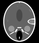
1 Phantom reference

2 QR reconstruction

3 Chest CT reference

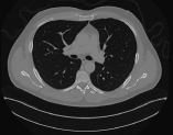
4 QR reconstruction

Figure 2: CT images

III-B Performance study

The computer used in the performance experiments featured one Intel i7-7800X® CPU (6 physical cores) and 128 GiB of RAM in total. The clock frequency of the processor was 3.50 GHz, and the so-called Max Turbo Frequency was 4.00 GHz. In addition to one small SSD for storing the operating system and programming tools, the computer had two disks that were employed in the experiments, both with a capacity of 2 TB: One Hard Disk Drive (HDD) and one Solid-State Drive (SSD) with an M.2 connector. The HDD (spinning disk) was a Toshiba DT01ACA200 (Firmware MX4OABB0). The SSD was a Samsung SSD 970 EVO 2TB (Firmware 1B2QEXE7). According to the Linux operating system hdparm tool, the read speed of the first one was about 191.43 MB/s, whereas the read speed of the second one was about was 2427.50 MB/s. This is an upper-middle desktop personal computer and its current price is only about a few thousand dollars. Its OS was GNU/Linux (kernel version 3.10.0-862.14.4.el7.x86_64). GCC compiler (version 4.8.5 20150623) was used. Intel(R) Math Kernel Library (MKL) Version 2018.0.2 Product Build 20180127 for Intel(R) 64 architecture was employed for solving some advanced linear algebra problems. Our new implementations were coded with the libflame (Release 11104) high-performance library, which employed Intel’s MKL for performing the small- and medium-sized basic linear algebra computations.

Because of the variability of the experimental running time on some computers, when solving linear systems three experiments were ran, and the average values were reported. Nevertheless, we must say that the three obtained times were similar on the assessed architecture. All the experiments reported show only the time required by the computation $X=R^{-1}(Q^{T}B)$, since the QR factorization can be computed only once and then employed for many different images.

Unless explicitly stated otherwise, all the experiments employed six threads (and therefore six cores) for computation since the computer had six cores, the only exception being the codes with overlapping of computation and I/O. In this case, five threads (and five cores) were employed for computation and one thread (one core) was employed for disk I/O tasks.

We have assessed four configurations, which are obtained as the combinations of two OOC AB methods (non-overlapping or basic OOC AB, and overlapping OOC AB) and two types of disks (HDD and SSD). The assessed four configurations were the following:

• B-OOC + HDD: The basic (or non-overlapping) Out-Of-Core Algorithm-by-Blocks for solving the linear system was employed on the HDD described above. This is also called the initial configuration.

• O-OOC + HDD: The Out-Of-Core Algorithm-by-Blocks with overlapping of computation and I/O for solving the linear system was employed on the HDD described above.

• B-OOC + SSD: The basic (or non-overlapping) Out-Of-Core Algorithm-by-Blocks for solving the linear system was employed on the SSD described above.

• O-OOC + SSD: The Out-Of-Core Algorithm-by-Blocks with overlapping of computation and I/O for solving the linear system was employed on the SSD described above.

In all our implementations we employed a block size 10240 for the OOC computations (the number of rows and columns of every square block, kept in a different file), since this size usually renders good results on all the assessed code variants [34, 32, 33]. In our codes, the block size employed inside every task to process the blocks once they are stored in RAM was 128, since this size usually renders good performances when processing matrices of size 10240. In the rest of the codes not developed by us (matrix-matrix products, etc.), the block size was determined by the library that performed that task (usually Intel’s MKL).

Figure 3: Overall times and decomposed times of the initial configuration (B-OOC + HDD) for solving a linear system with A of dimension $266,500\times 262,144$, and B of dimension $266,500\times k$, where $k$ is the number of slices.

Figure 3 shows the overall times and the decomposed times of the initial configuration (B-OOC + HDD, that is, the basic or non-overlapping OOC Algorithm-by-Blocks on the HDD) for solving a linear system with A of dimension $266,500\times 262,144$, and B of dimension $266,500\times k$, where $k$ is the number of slices. The aim of this plot was to assess if the process was feasible, and to determine the main bottleneck of the application. For the system with 2048 slices, 2.50 seconds per slice were needed; for the system with 256 slices, 14.54 seconds per slice were needed. These times showed that the process was feasible, but the times were a bit high in some cases and very high in other cases. Moreover, the decomposition of the time showed that I/O times were very high, but they did not grow too much as the number of slices increased. Therefore, the main bottleneck of this problem was the I/O time, instead of the computational time. Then, adding more cores or several GPUs to the hardware configuration was not going to help in this case, and the focus should instead be on a fast disk.

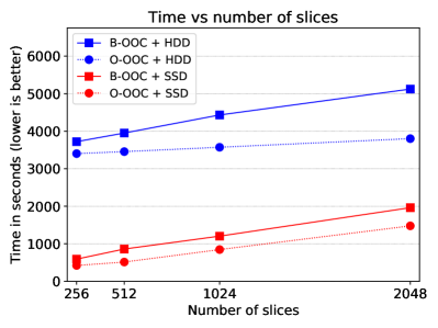
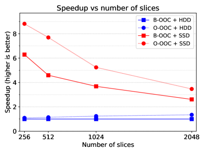
Figure 4: Time and speedups for the four configurations.

Figure 4 compares the performances of the four configurations described above: Basic OOC AB on HDD, Overlapping OOC AB on HDD, Basic OOC AB on SSD, and Overlapping OOC AB on SSD. The top subplot shows the times in seconds (lower is better), whereas the bottom subplot shows the speedup (higher is better) with respect to the initial configuration (basic OOC AB on HDD). The speedup is computed as the quotient of the time obtained by the reference configuration and the time obtained by the new configuration. Thus, this concept means how many times the new configuration is as fast as the reference configuration. Hence, the higher the speedups, the better the performances are. As the reference configuration is the initial one, in the bottom subplot the initial configuration will be shown as ones. As can be seen, the SSD greatly reduced the overall times and increased the speed by more than 6 times for the smallest case (256 slices) with respect to the initial configuration. The overlapping of computation and I/O further increased the speed up to nearly 9 times for the smallest case (256 slices). When the number of slices was high, the improvements were not so great but still very noticeable.

Figure 6 shows the overall times and the decomposed times for solving a linear system with A of dimension $266,500\times 262,144$, and B of dimension $266,500\times k$, where $k$ is the number of slices, on three configurations: B-OOC + HDD, B-OOC + SSD, and O-OOC + SSD. The left bar for each number of slices shows the overall times and the decomposed times of the initial configuration (B-OOC + HDD). As can be seen, its main drawback is the high I/O cost because of using a HDD. The center bar for each number of slices shows the overall times and the decomposed times of a configuration similar to the previous one with an SSD (B-OOC + SSD). As can be seen, the high I/O cost has been greatly reduced. The right bar for each number of slices shows the overall times of the best configuration (O-OOC + SSD). As this configuration overlaps computation and I/O, the time cannot be decomposed. As can be seen, in most cases the I/O cost (the fast SSD) of the previous configuration is completely removed.

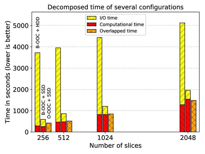
Figure 5: Overall times and decomposed times of three configurations for solving a linear system with A of dimension $266,500\times 262,144$, and B of dimension $266,500\times k$, where $k$ is the number of slices.

Figure 6: Time in seconds per slice for the four configurations.

Figure 6 shows the time in seconds required to compute one slice. As it shows, this time was not constant, and it depended somewhat on the number of slices: the more slices to compute, the lower the time per slice. Just consider that, regardless of the number of slices (even for just one slice), the whole factorized matrix $A$ must be read from disk. Thus, this large cost becomes diluted as more slices are being computed. In the initial configuration (basic OOC AB and HDD) the time per slice greatly depended on the number of slices. In the best configuration (overlapping OOC AB on SSD) the time per slice is not so dependent on the number of slices.

Table VI shows the time in seconds required to compute one slice for both the initial configuration and the most performant configuration.

As can be seen, the range of the initial configuration is very wide (from 2.50 to 14.54 seconds), whereas the range of the most performant configuration is much narrower (from 0.72 to 1.65 seconds).

The weights matrix for the highest resolution in our experimental study required a storage of about 560 GB ($265,500\times 262,144$ double precision elements). Besides the weights matrix, additional space (patient’s data, final image, temporary data, application code, operating system, disk buffers and cache, etc.) makes the total size required by this problem even larger. As was told, the computer had 128 GB of RAM. However, only 32 GB were employed as a cache to store blocks of the weights matrix, leaving the rest for other purposes (operating system disk cache and buffers, etc.). We assessed another computer with 48 GB of RAM, and results were similar when using a similar number of cores, but we did not report its results because it was a much more expensive server. Hence, to obtain good performances, a smaller main memory could be used (thus reducing the total price), but a fast SSD is a strong requirement.

TABLE VI: Time in seconds per slice versus number of slices.

	Number of slices
Method	256	512	1024	2048
B-OOC + HDD	14.54	7.72	4.33	2.50
O-OOC + SDD	1.65	1.00	0.83	0.72

IV Conclusions

In this paper, we present a direct algebraic method based on the QR factorization for reconstructing CT images efficiently on affordable computers. As we have shown, this method is numerically stable even for high resolutions provided the weights matrices have full rank. For this reason, our method employs more X-ray projections than the iterative methods, but fewer than the analytical methods. Besides, the use of few projections can affect the result of the diagnosis since some pathologies could be hidden or simulated.

With our proposed method, which uses a number of projections that guarantee the full rank of the weights matrix, high-quality images are obtained without requiring an a-priori knowledge or interaction with the patient. This method guarantees the non-creation of artifacts except those produced by problems on detectors, dispersion, movement, intensity of the source, etc., which can be corrected by filtering and segmentation techniques. In addition, our reconstructions achieve remarkable quality even for complex real CT images. It is worth to mention we have not considered or removed the possible noise on the projections, which is left as a future work.

We have shown that an efficient reconstruction of CT images can be achieved using Out-Of-Core and Algorithm-By-Blocks techniques. By using our techniques, affordable computers with a price of about one order of magnitude lower can be successfully employed, because a large main memory (which is quite expensive) is not required, just a fast hard drive. For this reason, the equipment needed to reconstruct the images is affordable and thus more accessible to the public. The type of hard drive can improve our reconstruction times drastically. When using a HDD, the performance is dominated by the I/O time, whereas when using an SSD the I/O time is greatly reduced and the performance is dominated by the computational time again. Furthermore, the method that overlaps computation and I/O can further reduce the reconstructing time, thus making our method more competitive. We could perform an standard CT study with resolution $512^{2}$ and 256 slices in about 4 minutes. We have also shown that the cost per slice is lower as the number of simultaneous slices to reconstruct is higher, which would be beneficial for full-body CT scans.

Considering all of the above, we conclude that computing high-quality reconstructions with direct algebraic methods on affordable equipment can be achieved. Since our method is stable we could increase the resolution of the images provided we had enough storage space, and still get valid results.

References

- [1] A. C. Kak and M. Slaney, Principles of Computerized Tomographic Imaging. SIAM, jan 2001, vol. 33.
- [2] A. B. De González, M. Mahesh, K.-P. Kim, M. Bhargavan, R. Lewis, F. Mettler, and C. Land, “Projected cancer risks from computed tomographic scans performed in the united states in 2007,” Archives of internal medicine, vol. 169, no. 22, pp. 2071–2077, 2009.
- [3] E. Hall and D. Brenner, “Cancer risks from diagnostic radiology,” The British journal of radiology, vol. 81, no. 965, pp. 362–378, 2008.
- [4] X. Tang, J. Hsieh, R. A. Nilsen, S. Dutta, D. Samsonov, and A. Hagiwara, “A three-dimensional-weighted cone beam filtered backprojection (CB-FBP) algorithm for image reconstruction in volumetric CT helical scanning,” Physics in Medicine & Biology, vol. 51, no. 4, p. 855, 2006.
- [5] T. Zhuang, S. Leng, B. E. Nett, and G.-H. Chen, “Fan-beam and cone-beam image reconstruction via filtering the backprojection image of differentiated projection data,” Physics in Medicine & Biology, vol. 49, no. 24, p. 5489, 2004.
- [6] S. Mori, M. Endo, S. Komatsu, S. Kandatsu, T. Yashiro, and M. Baba, “A combination-weighted Feldkamp-based reconstruction algorithm for cone-beam CT,” Physics in Medicine & Biology, vol. 51, no. 16, p. 3953, 2006.
- [7] M. J. Willemink, P. A. de Jong, T. Leiner, L. M. de Heer, R. A. Nievelstein, R. P. Budde, and A. M. Schilham, “Iterative reconstruction techniques for computed tomography part 1: technical principles,” European radiology, vol. 23, no. 6, pp. 1623–1631, 2013.
- [8] M. J. Willemink, T. Leiner, P. A. de Jong, L. M. de Heer, R. A. Nievelstein, A. M. Schilham, and R. P. Budde, “Iterative reconstruction techniques for computed tomography part 2: initial results in dose reduction and image quality,” European radiology, vol. 23, no. 6, pp. 1632–1642, 2013.
- [9] A. H. Andersen, “Algebraic reconstruction in CT from limited views,” IEEE Transactions on Medical Imaging, vol. 8, no. 1, pp. 50–55, 1989.
- [10] A. H. Andersen and A. C. Kak, “Simultaneous algebraic reconstruction technique (SART): a superior implementation of the ART algorithm,” Ultrasonic Imaging, vol. 6, no. 1, pp. 81–94, 1984.
- [11] W. Yu and L. Zeng, “A Novel Weighted Total Difference Based Image Reconstruction Algorithm for Few-View Computed Tomography,” PLoS ONE, vol. 9, no. 10, 2014.
- [12] L. Flores, V. Vidal, and G. Verdú, “Iterative reconstruction from few-view projections,” Procedia Computer Science, vol. 51, pp. 703–712, 2015.
- [13] L. A. Flores, V. Vidal, P. Mayo, F. Rodenas, and G. Verdú, “Parallel CT image reconstruction based on GPUs,” Radiation Physics and Chemistry, vol. 95, pp. 247–250, 2014.
- [14] M. Chillarón, V. Vidal, D. Segrelles, I. Blanquer, and G. Verdú, “Combining grid computing and Docker containers for the study and parametrization of CT image reconstruction methods,” Procedia Computer Science, vol. 108, pp. 1195–1204, 2017.
- [15] Yan Liu, Zhengrong Liang, Jianhua Ma, Hongbing Lu, Ke Wang, Hao Zhang, and W. Moore, “Total Variation-Stokes Strategy for Sparse-View X-ray CT Image Reconstruction,” IEEE Transactions on Medical Imaging, vol. 33, no. 3, pp. 749–763, mar 2014.
- [16] J. Tang, B. E. Nett, and G.-H. Chen, “Performance comparison between total variation (TV)-based compressed sensing and statistical iterative reconstruction algorithms,” Physics in Medicine and Biology, vol. 54, no. 19, pp. 5781–5804, oct 2009.
- [17] B. Vandeghinste, S. Vandenberghe, C. Vanhove, S. Staelens, and R. Van Holen, “Low-Dose Micro-CT Imaging for Vascular Segmentation and Analysis Using Sparse-View Acquisitions,” PLoS ONE, vol. 8, no. 7, p. e68449, jul 2013.
- [18] Z. Zhu, K. Wahid, P. Babyn, D. Cooper, I. Pratt, and Y. Carter, “Improved compressed sensing-based algorithm for sparse-view CT image reconstruction.” Computational and mathematical methods in medicine, vol. 2013, p. 185750, mar 2013.
- [19] I. Sechopoulos, “A review of breast tomosynthesis. Part II. Image reconstruction, processing and analysis, and advanced applications,” Medical physics, vol. 40, no. 1, 2013.
- [20] H. Qi, Z. Chen, and L. Zhou, “CT Image Reconstruction from Sparse Projections Using Adaptive TpV Regularization.” Computational and mathematical methods in medicine, vol. 2015, p. 354869, may 2015.
- [21] M. J. Rodríguez-Alvarez, F. Sanchez, A. Soriano, L. Moliner, S. Sanchez, and J. M. Benlloch, “QR-factorization Algorithm for Computed Tomography (CT): Comparison with FDK and Conjugate Gradient (CG) Algorithms,” IEEE Transactions on Radiation and Plasma Medical Sciences, vol. 2, no. 5, pp. 459–469, 2018.
- [22] M. Chillarón, V. Vidal, and G. Verdú, “CT image reconstruction with SuiteSparseQR factorization package,” Radiation Physics and Chemistry, 2019.
- [23] M. Chillarón, V. Vidal, G. Verdú, and J. Arnal, “CT Medical Imaging Reconstruction Using Direct Algebraic Methods with Few Projections,” in Computational Science – ICCS 2018. Cham: Springer International Publishing, 2018, pp. 334–346.
- [24] P. Joseph, “An improved algorithm for reprojecting rays through pixel images,” IEEE Transactions on Medical Imaging, vol. 1, no. 3, pp. 192–196, 1982.
- [25] A. Hore and D. Ziou, “Image Quality Metrics: PSNR vs. SSIM,” in 2010 20th International Conference on Pattern Recognition. IEEE, aug 2010, pp. 2366–2369.
- [26] S. Toledo and F. Gustavson, “The design and implementation of solar, a portable library for scalable out-of-core linear algebra computations,” Proceedings of the Annual Workshop on I/O in Parallel and Distributed Systems, IOPADS, 08 1998.
- [27] E. D’Azevedo and J. Dongarra, “Design and implementation of the parallel out-of-core ScaLAPACK LU, QR, and Cholesky factorization routines,” Concurrency - Practice and Experience, vol. 12, pp. 1481–1493, 12 2000.
- [28] W. C. Reiley and R. A. van de Geijn, “POOCLAPACK: Parallel Out-of-Core Linear Algebra Package,” Department of Computer Sciences, The University of Texas at Austin, Tech. Rep. CS-TR-99-33, 1999.
- [29] B. C. Gunter and R. A. van de Geijn, “Parallel out-of-core computation and updating the QR factorization,” ACM Transactions on Mathematical Software, vol. 31, no. 1, pp. 60–78, March 2005.
- [30] T. Joffrain, E. S. Quintana-Ortí, and R. A. van de Geijn, “Rapid development of high-performance out-of-core solvers,” in Proceedings of PARA 2004, ser. LNCS, no. 3732. Springer-Verlag Berlin Heidelberg, 2005, pp. 413–422.
- [31] B. C. Gunter, W. C. Reiley, and R. A. van de Geijn, “Parallel out-of-core Cholesky and QR factorizations with POOCLAPACK,” in Proceedings of the 15th International Parallel and Distributed Processing Symposium (IPDPS). IEEE Computer Society, 2001.
- [32] G. Quintana-Ortí, F. D. Igual, M. Marqués, E. S. Quintana-Ortí, and R. A. Van de Geijn, “A runtime system for programming out-of-core matrix algorithms-by-tiles on multithreaded architectures,” ACM Transactions on Mathematical Software (TOMS), vol. 38, no. 4, p. 25, 2012.
- [33] M. Marqués, G. Quintana-Ortí, E. S. Quintana-Ortí, and R. van de Geijn, “Using desktop computers to solve large-scale dense linear algebra problems,” The Journal of Supercomputing, vol. 58, no. 2, pp. 145–150, Nov 2011.
- [34] M. Marqués, G. Quintana-Ortí, E. S. Quintana-Ortí, and R. A. van de Geijn, “Out-of-Core Computation of the QR Factorization on Multi-core Processors,” in Lecture Notes in Computer Science 5704, Euro-Par’2009, (Eds. H. Sips, D. Epema, H. -X. Lin), 2009, pp. 809–820.
- [35] G. Lauritsch and H. Bruder, “FORBILD Head Phantom.” [Online]. Available: http://www.imp.uni-erlangen.de/phantoms/head/head.html
- [36] K. Yan, X. Wang, L. Lu, and R. M. Summers, “Deeplesion: automated mining of large-scale lesion annotations and universal lesion detection with deep learning,” Journal of Medical Imaging, vol. 5, no. 3, p. 036501, 2018.