Boundary properties of fractional objects:
flexibility of linear equations
and rigidity of minimal graphs

Abstract.

The main goal of this article is to understand the trace properties of nonlocal minimal graphs in $\mathbb{R}^{3}$, i.e. nonlocal minimal surfaces with a graphical structure.

We establish that at any boundary points at which the trace from inside happens to coincide with the exterior datum, also the tangent planes of the traces necessarily coincide with those of the exterior datum.

This very rigid geometric constraint is in sharp contrast with the case of the solutions of the linear equations driven by the fractional Laplacian, since we also show that, in this case, the fractional normal derivative can be prescribed arbitrarily, up to a small error.

We remark that, at a formal level, the linearization of the trace of a nonlocal minimal graph is given by the fractional normal derivative of a fractional Laplace problem, therefore the two problems are formally related. Nevertheless, the nonlinear equations of fractional mean curvature type present very specific properties which are strikingly different from those of other problems of fractional type which are apparently similar, but diverse in structure, and the nonlinear case given by the nonlocal minimal graphs turns out to be significantly more rigid than its linear counterpart.

1. Introduction

1.1. Boundary behavior of fractional objects

This article investigates the geometric properties at the boundary of solutions of fractional problems. Two similar, but structurally significantly different, situations are taken into account. On the one hand, we will consider the solution of the linear fractional equation

$$\begin{cases}(-\Delta)^{\sigma}u=0&{\mbox{ in }}B_{1}\cap\{x_{n}>0\},\\ u=0&{\mbox{ in }}\{x_{n}<0\},\end{cases}$$

where $\sigma\in(0,1)$, and, for $x^{\prime}=(x_{1},\dots,x_{n-1})$ with $|x^{\prime}|<1$, we consider the “fractional boundary derivative”

$$\lim_{x_{n}\searrow 0}\frac{u(x^{\prime},x_{n})}{x_{n}^{\sigma}}.$$ (1.1)

Interestingly, the function in (1.1) plays an important role in understanding fractional equations, see [MR3168912]. In particular, while classical elliptic equations are smooth up to the boundary, the solutions of fractional equations with prescribed exterior datum are in general not better than Hölder continuous with exponent $\sigma$, and therefore the function in (1.1) is the crucial ingredient to detect the growth of the solution in the vicinity of the boundary.

As a first result, we will show here that, roughly speaking, the function in (1.1) can be arbitrarily prescribed, up to an arbitrarily small error. That is, one can construct solutions of linear fractional equations whose fractional boundary derivative behaves in an essentially arbitrary way.

Then, we turn our attention to the boundary property of nonlocal minimal graphs, i.e. minimizers of the fractional perimeter functional which possess a graphical structure. In this case, we show that the boundary properties are subject to severe geometric constraints, in sharp contrast with the case of fractional equations.

First of all, the continuity properties of nonlocal minimal graphs are very different from those of the solutions of fractional equations, since we have established in [MR3516886, MR3596708] that nonlocal minimal graphs are not necessarily continuous at the boundary. In addition, the boundary discontinuity of nonlocal minimal graphs in the plane happens to be a “generic” situation, as we have recently proved in [2019arXiv190405393D].

The focus of this article is on the three-dimensional setting, i.e. the case in which the graph is embedded in $\mathbb{R}^{3}$. In this situation, the graph can be continuous at a given point, but the discontinuity may occur along the trace, at nearby points. More precisely, we will look at a function $u:\mathbb{R}^{2}\to\mathbb{R}$, which is an $s$-minimal graph in $(-2,2)\times(0,4)$ and is such that $u=0$ in $(-2,2)\times(-h,0)$, for some $h>0$. In this setting, we will consider its trace along $\{x_{2}=0\}$, namely we consider the function

$$\lim_{x_{2}\searrow 0}u(x_{1},x_{2}).$$

The main question that we address in this article is precisely whether or not the trace of a nonlocal minimal graph possesses any distinctive feature or satisfies any particular geometric constraint.

We will prove that, differently from the case of the linear equations (and also in sharp contrast to the case of classical minimal surfaces), the traces of nonlocal minimal graphs cannot have an arbitrary shape, and, in fact, matching points from the two sides must necessarily occur with horizontal tangencies.

This result relies on a classification theory for homogeneous graphs, since we will show that, in this case, the matching at the origin is sufficient to make a nonlocal minimal graph trivial.

In the rest of this introduction, we will present the precise mathematical framework in which we work and provide the formal statements of our main results.

1.2. Boundary flexibility of linear fractional equations

We discuss now the case of fractional linear equations, showing that the fractional boundary derivative of the solutions can be essentially arbitrarily prescribed, up to a small error. For this, we denote by $B^{\prime}_{r}$ the $(n-1)$-dimensional ball of radius $r$ centered at the origin, namely

$$B^{\prime}_{r}:=\{x^{\prime}\in\mathbb{R}^{n-1}{\mbox{ s.t. }}|x^{\prime}|<r\}.$$

As customary, given $\sigma\in(0,1)$, we define the fractional Laplacian as

$$(-\Delta)^{\sigma}u(x):=\int_{\mathbb{R}^{n}}\frac{2u(x)-u(x+y)-u(x-y)}{|y|^{n+\sigma}}\,dy.$$

Then, we have:

Theorem 1.1.

Let $n\geqslant 2$, $\sigma\in(0,1)$, $k\in\mathbb{N}$ and $f\in C^{k}(\overline{B_{1}^{\prime}})$. Then, for every $\varepsilon>0$ there exist $f_{\varepsilon}\in C^{k}(\mathbb{R}^{n-1})$ and $u_{\varepsilon}\in C(\mathbb{R}^{n})$ such that

$$\begin{cases}(-\Delta)^{\sigma}u_{\varepsilon}=0&{\mbox{ in }}B_{1}\cap\{x_{n}>0\},\\ u_{\varepsilon}=0&{\mbox{ in }}\{x_{n}<0\},\end{cases}$$ (1.2)

$$\lim_{x_{n}\searrow 0}\frac{u_{\varepsilon}(x^{\prime},x_{n})}{x_{n}^{\sigma}}=f_{\varepsilon}(x^{\prime})\qquad{\mbox{ for all }}x^{\prime}\in B_{1}^{\prime},$$ (1.3)

and

$$\|f_{\varepsilon}-f\|_{C^{k}(\overline{B_{1}^{\prime}})}\leqslant\varepsilon.$$ (1.4)

On the one hand, Theorem 1.1 falls in the research line opened in [MR3626547] according to which “all functions are $\sigma$-harmonic up to a small error”, namely it states an interesting flexibility offered by solutions of fractional equations which can adapt themselves in order to capture essentially any prescribed behavior. This flexible feature has been recently studied in several fractional contexts, including time-fractional derivatives, non-elliptic operators, and higher order operators, see [MR3716924, MR3935264, KRYL, CAR, CARBOO]. In addition, the flexible properties of fractional equations can be effectively exploited to construct interesting counterexamples, see [MR3783214], and they have consequences in concrete scenarios involving also mathematical biology and inverse problems, see [MR3579567, MR3774704]. Differently from the previous literature, Theorem 1.1 aims at detecting a “boundary” flexibility of fractional equations, rather than an “interior” one.

On the other hand, differently from all the other fractional flexibility results in the literature, which have no counterpart for the case of the classical Laplacian, Theorem 1.1 shares a common treat with the Laplace equation and possesses a full classical analogue (we present its classical counterpart in Appendix A).

1.3. Boundary rigidity of fractional minimal surfaces

We now discuss the boundary behavior of $s$-minimal surfaces and we will show its striking differences with respect to the linear fractional equations. To this end, we recall the setting introduced in [MR2675483]. Given $s\in(0,1)$, we consider the interaction of two disjoint (measurable) sets $F$, $G\subseteq\mathbb{R}^{N}$ defined by

$${\mathcal{I}}_{s}(F,G):=\iint_{F\times G}\frac{dx\,dy}{|x-y|^{N+s}}.$$ (1.5)

Given a bounded reference domain $\Omega$ with Lipschitz boundary, we define the $s$-perimeter of a set $E\subseteq\mathbb{R}^{N}$ in $\Omega$ by

$${\rm Per}_{s}(E;\Omega):={\mathcal{I}}_{s}(E\cap\Omega,E^{c}\cap\Omega)+{\mathcal{I}}_{s}(E\cap\Omega,E^{c}\cap\Omega^{c})+{\mathcal{I}}_{s}(E\cap\Omega^{c},E^{c}\cap\Omega).$$

As customary, we have used here the complementary set notation $E^{c}:=\mathbb{R}^{N}\setminus E$.

Definition 1.2.

Let $\Omega\subset\mathbb{R}^{N}$ be bounded and with Lipschitz boundary. Let $E\subseteq\mathbb{R}^{N}$. We say that $E$ is $s$-minimal in $\Omega$ if ${\rm Per}_{s}(E;\Omega)<+\infty$ and

$${\rm Per}_{s}(E;\Omega)\leqslant{\rm Per}_{s}(E^{\prime};\Omega)$$ (1.6)

for every $E^{\prime}\subseteq\mathbb{R}^{N}$ such that $E^{\prime}\cap\Omega^{c}=E\cap\Omega^{c}$.

Moreover, given $U\subset\mathbb{R}^{N}$, we say that $E$ is locally $s$-minimal in $U$ if it $s$-minimal in $\Omega$, for every $\Omega$ which is bounded, with Lipschitz boundary and strictly contained in $U$.

We remark that one can make sense of the minimization procedure also in unbounded domains by saying that $E$ is locally $s$-minimal in a (possibly unbounded) domain $\Omega$ if $E$ is $s$-minimal in every bounded and Lipschitz domain $\Omega^{\prime}\Subset\Omega$ (see Section 1.3 in [MR3827804] for additional details on these minimality notions).

The regularity theory of nonlocal minimal surfaces is a fascinating topic of investigation, still possessing a number of fundamental open problems. We refer to [MR3090533, MR3107529, MR3331523, BV] for interior regularity results, [MR3798717, CCC] for a precise discussion on stable nonlocal cones, and [MR3588123, MR3824212] for recent surveys containing the state of the art of this problem.

A particularly important case of locally $s$-minimal sets is given by the ones which have a graph structure. Namely, given $\Omega_{0}\subseteq\mathbb{R}^{n}$ and $u:\Omega_{0}\to\mathbb{R}$, we let

$$E_{u}:=\{X=(x,x_{n+1}){\mbox{ s.t. $x\in\Omega_{0}$ and $x_{n+1}<u(x)$}}\}.$$ (1.7)

With respect to the notation in (1.5), we are taking here $N=n+1$.

Definition 1.3.

We say that $u$ is an $s$-minimal graph in $\Omega_{0}$ if $E_{u}$ is a locally $s$-minimal set in $\Omega_{0}\times\mathbb{R}$.

Interestingly, $s$-minimal graphs enjoy suitable Bernstein-type properties, see [MR3680376, PISA, 2018arXiv180705774C], and they have a smooth interior regularity theory, as proved in [MR3934589].

See also [NOCHETTO] for several very precise simulations on nonlocal minimal graphs and a sharp numerical analysis of their properties.

With this, we are ready to state the main result of this article, which gives some precise geometric conditions on the trace of nonlocal minimal graphs. We establish that the trace graph has necessarily zero derivatives when the trace crosses zero. The precise result that we have is the following one:

Theorem 1.4.

Let $u$ be an $s$-minimal graph in $(-2,2)\times(0,4)$. Assume that there exists $h>0$ such that $u=0$ in $(-2,2)\times(-h,0)$, and let

$$f(x_{1}):=\lim_{x_{2}\searrow 0}u(x_{1},x_{2}).$$ (1.8)

Then, there exist $\delta_{0}\in\left(0,\frac{1}{100}\right)$ and $C>0$ such that if $\zeta_{0}\in\left(-\frac{3}{2},\frac{3}{2}\right)$ is such that $f(\zeta_{0})=0$, then

$$|u(x)|\leqslant C\,|x-(\zeta_{0},0)|^{\frac{3+s}{2}}$$ (1.9)

for every $x\in B_{\delta_{0}}(\zeta_{0},0)$, and, in particular,

$$f^{\prime}(\zeta_{0})=0$$. (1.10)

We remark that the existence of the limit in (1.8) is warranted by Theorem 1.1 in [MR3516886].

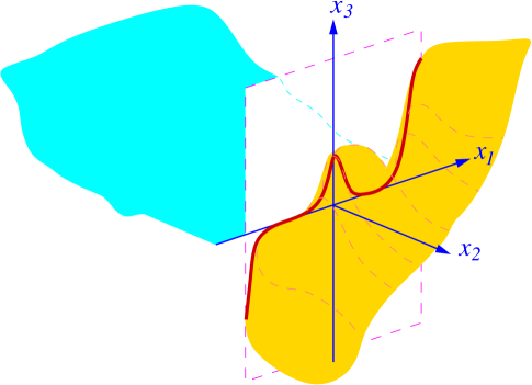
Figure 1. A nonlocal minimal graph, in the light of Theorem 1.4. The red curve represents the graph of the function $f$ defined in (1.8).

The statement of Theorem 1.4 is described in Figures 1 and 2. With respect to this, we stress the remarkable geometric property given by the vanishing of the gradient of the trace at the zero crossing points. We observe that this situation is completely different with respect to the one arising for solutions of linear equations, and one can compare the structurally “rigid” geometry imposed by Theorem 1.4 with the almost completely arbitrariness arising in Theorem 1.1.

We remark that, at a formal level, the settings in Theorems 1.1 and 1.4 are strictly related, since the linearization of the trace of a nonlocal minimal graph is given by the fractional normal derivative of a fractional Laplace problem. More specifically, when one takes into account the improvement of flatness argument for an $\varepsilon$-flat nonlocal minimal graph $u$ (see the forthcoming Lemma 5.1), one sees that $u/\varepsilon$ shadows a function $\bar{u}$, which is a solution of $(-\Delta)^{\sigma}\bar{u}=0$ in $\{x_{2}>0\}$, with $\sigma:=\frac{1+s}{2}$: in this context the first order of $\bar{u}$ near the origin takes the form $\bar{a}\,x_{2}^{\sigma}$, for some $a\in\mathbb{R}$. Comparing with (1.3), one has that $\bar{a}$ is exactly the fractional normal derivative of the solution of a linear equation, which, in view of Theorem 1.1, can be prescribed in an essentially arbitrary way.

In this spirit, if the linearization procedure produced a “good approximation” of the nonlinear geometric problem, one would expect that the original nonlocal minimal graph $u$ is well approximated near the origin by a term of the form $\varepsilon\,\bar{a}\,x_{2}^{\sigma}$, with no prescription whatsoever on $\bar{a}$. Quite surprisingly, formula (1.9) (applied here with $\zeta_{0}:=0$) tells us that this is not the case, and the correct behavior of a nonlocal minimal graph at the boundary cannot be simply understood “by linearization”.

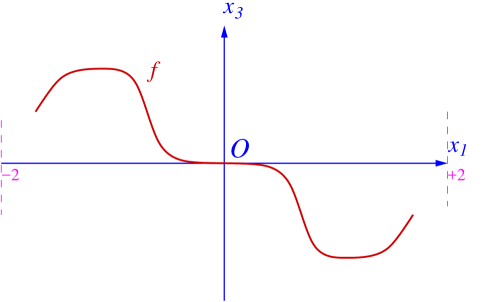
Figure 2. How we expect the graph of the function $f$ defined in (1.8) when $n=2$ and the exterior datum is $$u(x):=\chi_{(-2,0)\times(-1,-3)}(x)-\chi_{(0,2)\times(-1,-3)}$$ for all $x\in\mathbb{R}^{2}\setminus\big{(}(-2,2)\times(0,4)\big{)}$. Notice the horizontal tangency at the origin.

Theorem 1.4 also reveals a structural difference of the boundary regularity theory of fractional minimal surfaces embedded in $\mathbb{R}^{n+1}$ when $n=2$ with respect to the case in which $n=1$. Indeed, when $n=1$, an $s$-minimal graph in which the exterior datum is attained continuously at a boundary point is necessarily $C^{1,\frac{1+s}{2}}$ in a neighborhood of such a point (see Theorem 1.2 in [2019arXiv190405393D]). Instead, when $n=2$, a similar result does not hold: as a matter of fact, when $n=2$,

• Theorem 1.4 guarantees that boundary points which attain the flat exterior datum in a continuous way have necessarily horizontal tangency,

• conversely, boundary points in which the $s$-minimal graph experience a jump have necessarily a vertical tangency (see [MR3532394]).

Consequently, points with vertical tangency accumulate to zero crossing points possessing horizontal tangency, preventing a differentiable boundary regularity of the surface in a neighborhood of the latter type of points.

The proof of Theorem 1.4 will require a fine understanding of fractional minimal homogeneous graphs. Indeed, as a pivotal step towards the proof of Theorem 1.4, we establish the surprising feature that if a homogeneous fractional locally minimal graph vanishes in $\{x_{n}<0\}$ and it is continuous at the origin, then it necessarily vanishes at all points of $\{x_{n}=0\}$. The precise result that we obtain is the following:

Theorem 1.5.

Let $u$ be an $s$-minimal graph in $\mathbb{R}\times(0,+\infty)$. Assume that

$$u(x_{1},x_{2})=0 x_{2}<0$$ if . (1.11)

Assume also that $u$ is positively homogeneous of degree $1$, i.e.

$$u(tx)=tu(x)\qquad{\mbox{ for all $x\in\mathbb{R}^{2}$ and\leavevmode\nobreak\ $t>0$.}}$$ (1.12)

Suppose that

$$u(0):=\lim_{x\to 0}u(x)=0.$$ (1.13)

Then $u(x)=0$ for all $x\in\mathbb{R}^{2}$.

We take this opportunity to state and discuss some new interesting research lines opened by the results obtained in the present paper.

Open Problem 1.6 (Vertical tangencies).

In the setting of Theorem 1.4, can one construct examples in which $f^{\prime}(\zeta)=\pm\infty$ for some $\zeta\in\left(-\frac{3}{2},\frac{3}{2}\right)$?

Namely, is it possible to construct examples of nonlocal minimal graphs embedded in $\mathbb{R}^{3}$ which are flat from outside and whose trace develops vertical tangencies?

The trace of such possible pathological examples is depicted in Figure 3.

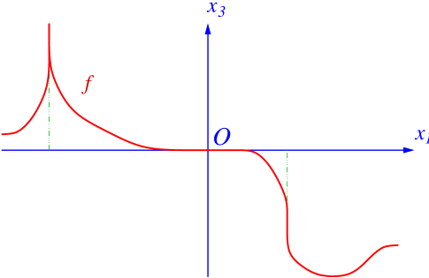
Figure 3. Open problem 1.6: is it possible to construct nonlocal minimal graphs traces with vertical tangencies?

Open Problem 1.7 (The higher dimensional case).

It would be interesting to determine whether or not a result similar to Theorem 1.4 holds true in higher dimension. Similarly, it would be interesting to determine the possible validity of Theorem 1.5 in higher dimensions.

From the technical point of view, we observe that some of the auxiliary results exploited towards the proof of Theorem 1.5 (such as Lemma 3.5 and Corollary 3.7) are expected to carry over in higher dimension, therefore one can in principle try to argue by induction, supposing that a statement such as the one of Theorem 1.5 holds true in dimension $n$ with the aim of proving it in dimension $n+1$. The catch in this argument is that one is led to study the points at which the gradient of the trace attains its maximal, and this makes an important connection between this line of research and that of Open Problem 1.6.

Open Problem 1.8 (Behavior at a corner of the domain).

It would be interesting to detect the behavior of a nonlocal minimal graph and of its trace at the corners of the domain and in their vicinity, in particular understanding (dis)continuity and tangency properties, possibly also in relation with the convexity or concavity of the corner. This is related to the analysis of nonlocal minimal cones in either convex or concave sectors with zero exterior datum.

As a first step towards it, one can try to understand how to complete Figure 2 near $x_{1}=\pm 2$.

1.4. Organization of the paper

The rest of this manuscript is organized as follows. Theorem 1.1 is proved in Section 2. The arguments used will exploit a method that we have recently introduced in [MR3626547] to show that “all functions are locally fractional harmonic”, and a careful discussion of the homogeneous solutions of fractional equations on cones, see [MR2075671, MR3810469].

Then, in Section 3 we present the proof of Theorem 1.5. The arguments used here exploit and develop a series of fine methods from the theory of nonlocal equations, comprising boundary Lipschitz bounds, blow-up classification results, continuity implies differentiability results, nonlocal geometric equations and nonlocal obstacle-type problems.

In Section 4 we construct a useful barrier, that we exploit to rule out the case of boundary Lipschitz singularities for nonlocal minimal graphs.

The proof of Theorem 1.4 is contained in Section 5. Finally, in Appendix A, we point out the classical analogue of Theorem 1.1.

2. Proof of Theorem 1.1

One important ingredient towards the proof of Theorem 1.1 consists in the construction of a homogeneous solution of a linear fractional equation with a suitable growth from the vertex of a cone. This is indeed a classical topic of research, which also bridges mathematical analysis and probability, see [MR1936081, MR2075671, MR3810469] for specific results on fractional harmonic functions on cones. In our setting, we can reduce to the two-dimensional case (though the higher dimensional case can be treated in a similar way), and, for any $\alpha>0$, we let

$${\mathcal{C}}_{\alpha}:=\left\{x=(x_{1},x_{2})\in\mathbb{R}^{2}{\mbox{ s.t. $x_{2}>0$ and $x_{1}+\displaystyle\frac{x_{2}}{\alpha}>0$}}\right\},$$ (2.1)

and the result that we need is the following one:

Lemma 2.1.

For every $\sigma\in(0,1)$ and every $\vartheta\in\mathbb{R}$ there exist $\alpha>0$, $\beta\in(0,2\sigma)\setminus\{\vartheta\}$ and $\bar{v}:S^{1}\to[0,+\infty)$ with $\|\bar{v}\|_{L^{\infty}(S^{1})}=1$ such that the function

$$\mathbb{R}^{2}\ni x\mapsto v(x):=|x|^{\beta}\,\bar{v}\left(\frac{x}{|x|}\right)$$ (2.2)

satisfies

$$\begin{cases}(-\Delta)^{\sigma}v=0&{\mbox{ in }}{\mathcal{C}}_{\alpha},\\ v=0&{\mbox{ in }}\mathbb{R}^{2}\setminus{\mathcal{C}}_{\alpha}.\end{cases}$$ (2.3)

Proof.

Let $\vartheta\in\mathbb{R}$. By Theorem 3.2 in [MR2075671], for every $\alpha>0$ there exist $\beta(\alpha)\in(0,2\sigma)$ and $\bar{v}_{\alpha}:S^{1}\to[0,+\infty)$ with $\|\bar{v}_{\alpha}\|_{L^{\infty}(S^{1})}=1$ such that the function

$$\mathbb{R}^{n}\ni x\mapsto v_{\alpha}(x):=|x|^{\beta}\,\bar{v}_{\alpha}\left(\frac{x}{|x|}\right)$$

satisfies

$$\begin{cases}(-\Delta)^{\sigma}v_{\alpha}=0&{\mbox{ in }}{\mathcal{C}}_{\alpha},\\ v_{\alpha}=0&{\mbox{ in }}\mathbb{R}^{2}\setminus{\mathcal{C}}_{\alpha}.\end{cases}$$

Let us focus on the case $\alpha=1$. If $\beta(1)\neq\vartheta$, then the claims of Lemma 2.1 are satisfied by choosing $\alpha:=1$, $\beta:=\beta(1)$ and $\bar{v}:=\bar{v}_{1}$.

If instead $\beta(1)=\vartheta$, we exploit Lemma 3.3 in [MR2075671]. Namely, since ${\mathcal{C}}_{1/2}\supset{\mathcal{C}}_{1}$, we deduce from Lemma 3.3 in [MR2075671] that $\beta(1/2)<\beta(1)=\vartheta$, and thus the claims of Lemma 2.1 are satisfied in this case by choosing $\alpha:=1/2$, $\beta:=\beta(1/2)$ and $\bar{v}:=\bar{v}_{1/2}$. ∎

Exploiting Lemma 2.1, we will obtain that the boundary derivatives of $\sigma$-harmonic functions have maximal span. For this, given $k\in\mathbb{N}$, we define by ${\mathcal{H}}_{k}$ the set of all functions $u\in C(\mathbb{R}^{n})$ for which there exists $r>0$ such that

$$\begin{cases}(-\Delta)^{\sigma}u=0&{\mbox{ in }}B_{r}\cap\{x_{n}>0\},\\ u=0&{\mbox{ in }}\{x_{n}<0\},\end{cases}$$ (2.4)

and for which there exists $\phi\in C^{k}(\overline{B^{\prime}_{r}})$ such that

$${\mathcal{T}}u(x^{\prime}):=\lim_{x_{n}\searrow 0}\frac{u(x^{\prime},x_{n})}{x_{n}^{\sigma}}=\phi(x^{\prime})\qquad{\mbox{ for all }}x^{\prime}\in B_{r}^{\prime}.$$

Also, given $r>0$ and $\phi\in C^{k}(\overline{B^{\prime}_{r}})$, we consider the array

$${\mathcal{D}}^{k}\phi(0):=\big{(}D^{\gamma}\phi(0)\big{)}_{{\gamma\in\mathbb{N}^{n-1}}\atop{|\gamma|\leqslant k}}\;.$$ (2.5)

Namely, the array ${\mathcal{D}}^{k}\phi(0)$ contains all the derivatives of $\phi$ at the origin, up to order $k$. Fixing some order in the components of the multiindex, we can consider ${\mathcal{D}}^{k}\phi(0)$ as a vector in $\mathbb{R}^{N_{k}}$, with

$$N_{k}:=\sum_{j=0}^{k}(n-1)^{j}.$$ (2.6)

The following result states that the linear space produced in this way is “as large as possible”:

Lemma 2.2.

We have that

$$\Big{\{}{\mathcal{D}}^{k}\phi(0),{\mbox{ with }}\phi={\mathcal{T}}u{\mbox{ and }}u\in{\mathcal{H}}_{k}\Big{\}}=\mathbb{R}^{N_{k}}.$$ (2.7)

Proof.

Suppose, by contradiction, that the linear space in the left hand side of (2.7) does not exhaust the whole of $\mathbb{R}^{N_{k}}$. Then, there would exist

$$\omega\in\mathbb{R}^{N_{k}}\setminus\{0\}$$ (2.8)

such that the linear space in the left hand side of (2.7) lies in the orthogonal space of $\omega$. Namely, for every $u\in{\mathcal{H}}_{k}$ with $\phi={\mathcal{T}}u$,

$${\mathcal{D}}^{k}\phi(0)\cdot\omega=0.$$ (2.9)

Recalling the notation in (2.5), we can write $\omega=(\omega_{\gamma})_{{\gamma\in\mathbb{N}^{n-1}}\atop{|\gamma|\leqslant k}}$, and then (2.9) takes the form

$$\sum_{{\gamma\in\mathbb{N}^{n-1}}\atop{|\gamma|\leqslant k}}\omega_{\gamma}\,D^{\gamma}\phi(0)=0,\qquad{\mbox{ for all\leavevmode\nobreak\ $u\in{\mathcal{H}}_{k}$ with\leavevmode\nobreak\ $\phi={\mathcal{T}}u$. }}$$ (2.10)

Now, we exploit Lemma 2.1 with $\vartheta:=\sigma$. In the notation of Lemma 2.1, we take $P=(P_{1},P_{2})\in{\mathcal{C}}_{\alpha}\subset\mathbb{R}^{2}$ such that $v(P)>0$ and define

$$\tilde{v}(x_{1},x_{2}):=\frac{v(P)\;x_{2}^{\sigma}}{P_{2}^{\sigma}}.$$

We observe that $\tilde{v}(P)=v(P)$. Accordingly, by the Boundary Harnack Inequality (see Theorem 1 on page 44 of [MR1438304]), we have that, for all $\varepsilon>0$,

$$\left[\frac{1}{C},C\right]\ni\Lambda:=\lim_{x_{n}\searrow 0}\frac{v(\varepsilon,x_{n})}{\tilde{v}(\varepsilon,x_{n})}=\lim_{\tau\searrow 0}\frac{P_{2}^{\sigma}\;v(\varepsilon,\tau)}{v(P)\;\tau^{\sigma}},$$ (2.11)

for some $C\geqslant 1$.

Now, for all $\varepsilon>0$ and $\zeta\in S^{n-2}$ we define

$$w(x):=v(x^{\prime}\cdot\zeta+\varepsilon,x_{n}).$$ (2.12)

Also, if $r:=\frac{\varepsilon}{2}$ and $x\in B_{r}\cap\{x_{n}>0\}$, it follows that $x^{\prime}\cdot\zeta+\varepsilon+\frac{x_{n}}{\alpha}\geqslant-r+\varepsilon>0$, and thus $(x^{\prime}\cdot\zeta+\varepsilon,x_{n})\in{\mathcal{C}}_{\alpha}$. Consequently, by (2.3), we have that

$$(-\Delta)^{\sigma}w=0 B_{r}\cap\{x_{n}>0\}$$ in . (2.13)

Moreover, using (2.3) and (2.12), we see that

if $$x_{n}<0 w(x)=0$$ then . (2.14)

From (2.13) and (2.14) (see e.g. Section 1.1 in [MR3694738], or [MR3293447, MR3276603]), it also follows that the function ${\rm dist}_{\{x_{n}<0\}}^{-\sigma}w$ belongs to $C^{\infty}(B_{r}\cap\overline{\{x_{n}>0\}})$, hence we can define

$$\psi(x^{\prime}):=\lim_{x_{n}\searrow 0}\frac{w(x^{\prime},x_{n})}{{\rm dist}_{\{x_{n}<0\}}^{\sigma}(x^{\prime},x_{n})}=\lim_{x_{n}\searrow 0}\frac{w(x^{\prime},x_{n})}{x_{n}^{\sigma}}={\mathcal{T}}w(x^{\prime}).$$ (2.15)

This, (2.13) and (2.14) give that $w\in{\mathcal{H}}_{k}$. As a consequence, recalling (2.10), we have that

$$\sum_{{\gamma\in\mathbb{N}^{n-1}}\atop{|\gamma|\leqslant k}}\omega_{\gamma}\,D^{\gamma}\psi(0)=0.$$ (2.16)

In view of (2.12) and (2.15), we also observe that

$$\psi(x^{\prime})=\lim_{x_{n}\searrow 0}\frac{v(x^{\prime}\cdot\zeta+\varepsilon,x_{n})}{x_{n}^{\sigma}}.$$ (2.17)

Accordingly, recalling (2.11),

$$\psi(0)=\lim_{x_{n}\searrow 0}\frac{v(\varepsilon,x_{n})}{x_{n}^{\sigma}}=\frac{\Lambda\,v(P)}{P_{2}^{\sigma}}=:\tilde{\Lambda}\neq 0.$$ (2.18)

Also, by (2.17), we can write that

$$\psi(x^{\prime})=\psi_{0}(x^{\prime}\cdot\zeta),$$ (2.19)

for some $\psi_{0}:\mathbb{R}\to[0,+\infty)$. Hence, recalling the homogeneity in (2.2), for all $t>0$,

$$\psi_{0}\big{(}t(x^{\prime}\cdot\zeta+\varepsilon)-\varepsilon\big{)}=\psi\big{(}t(x^{\prime}+\varepsilon\zeta)-\varepsilon\zeta\big{)}=\lim_{x_{n}\searrow 0}\frac{v\big{(}(t(x^{\prime}+\varepsilon\zeta)-\varepsilon\zeta)\cdot\zeta+\varepsilon,x_{n}\big{)}}{x_{n}^{\sigma}}$$

$$\qquad=\lim_{x_{n}\searrow 0}\frac{v(tx^{\prime}\cdot\zeta+t\varepsilon,x_{n})}{x_{n}^{\sigma}}=\lim_{y_{n}\searrow 0}\frac{v\big{(}t(x^{\prime}\cdot\zeta+\varepsilon),ty_{n}\big{)}}{t^{\sigma}y_{n}^{\sigma}}=\lim_{y_{n}\searrow 0}\frac{t^{\beta}v(x^{\prime}\cdot\zeta+\varepsilon,y_{n})}{t^{\sigma}y_{n}^{\sigma}}$$

$$\qquad=t^{\beta-\sigma}\psi(x^{\prime})=t^{\beta-\sigma}\psi_{0}(x^{\prime}\cdot\zeta)$$

Taking $m$ derivatives in $t$ of this identity, we conclude that

$$\psi_{0}^{(m)}\big{(}t(x^{\prime}\cdot\zeta+\varepsilon)-\varepsilon\big{)}\,(x^{\prime}\cdot\zeta+\varepsilon)^{m}=\prod_{i=0}^{m-1}(\beta-\sigma-i)\;t^{\beta-\sigma-m}\,\psi_{0}(x^{\prime}\cdot\zeta).$$ (2.20)

In addition, by (2.19), we have that $D^{\gamma}\psi(x^{\prime})=\zeta^{\gamma}\psi_{0}^{(|\gamma|)}(x^{\prime}\cdot\zeta)$. Hence, evaluating (2.20) at $t:=1$ and $x^{\prime}:=0$, if $m=|\gamma|$ we have that

$$\begin{split}&\varepsilon^{m}D^{\gamma}\psi(0)=\zeta^{\gamma}\psi_{0}^{(m)}(0)\,\varepsilon^{m}=\zeta^{\gamma}\kappa_{m}\,\psi_{0}(0)=\zeta^{\gamma}\kappa_{m}\,\psi(0),\\ {\mbox{where }}\qquad&\kappa_{m}:=\prod_{i=0}^{m-1}(\beta-\sigma-i).\end{split}$$ (2.21)

Plugging this information into (2.16), and recalling (2.18), we find that

$$\begin{split}&0=\frac{1}{\tilde{\Lambda}}\sum_{m=1}^{k}\sum_{{\gamma\in\mathbb{N}^{n-1}}\atop{|\gamma|=m}}\omega_{\gamma}\,D^{\gamma}\psi(0)=\frac{1}{\tilde{\Lambda}}\sum_{m=1}^{k}\sum_{{\gamma\in\mathbb{N}^{n-1}}\atop{|\gamma|=m}}\kappa_{m}\,\varepsilon^{-m}\omega_{\gamma}\zeta^{\gamma}\psi(0)\\ &\qquad\qquad=\frac{1}{\tilde{\Lambda}}\sum_{{\gamma\in\mathbb{N}^{n-1}}\atop{|\gamma|\leqslant k}}\kappa_{|\gamma|}\,\omega_{\gamma}\left(\frac{\zeta}{\varepsilon}\right)^{\gamma}\psi(0)=\sum_{{\gamma\in\mathbb{N}^{n-1}}\atop{|\gamma|\leqslant k}}\kappa_{|\gamma|}\,\omega_{\gamma}\left(\frac{\zeta}{\varepsilon}\right)^{\gamma}.\end{split}$$ (2.22)

Since $\frac{\zeta}{\varepsilon}$ ranges in an open set of $\mathbb{R}^{n-1}$, we deduce from (2.22) and the Identity Principle for polynomials that $\kappa_{|\gamma|}\,\omega_{\gamma}=0$ for all $\gamma\in\mathbb{N}^{n-1}$ with $|\gamma|\leqslant k$. As a consequence, by (2.21), we find that $\omega_{\gamma}=0$ for all $\gamma\in\mathbb{N}^{n-1}$ with $|\gamma|\leqslant k$, hence $\omega=0$. This is in contradiction with (2.8) and thus we have proved the desired result. ∎

With this, we are in the position of completing the proof of Theorem 1.1 by arguing as follows:

Proof of Theorem 1.1.

Since the claims in Theorem 1.1 have a linear structure in $f$, $f_{\varepsilon}$ and $u_{\varepsilon}$, by the Stone-Weierstraß Theorem, it is enough to prove Theorem 1.1 if $f$ is a monomial. Hence, we fix $\varepsilon\in(0,1)$, possibly to be taken conveniently small, and we suppose that

$$f(x^{\prime})=\frac{(x^{\prime})^{\mu}}{\mu!}\qquad{\mbox{for some }}\mu\in\mathbb{N}^{n-1}.$$ (2.23)

Then, we apply Lemma 2.2, finding a suitable function $u_{\star}\in{\mathcal{H}}_{k}$ with $\phi_{\star}:={\mathcal{T}}u_{\star}$ that satisfies

$$D^{\gamma}\phi_{\star}(0)=\begin{cases}1&{\mbox{ if }}\gamma=\mu,\\ 0&{\mbox{ if $|\gamma|\leqslant|\mu|+k$ and\leavevmode\nobreak\ $\gamma\neq\mu$.}}\end{cases}$$ (2.24)

We define

$$u_{\varepsilon}(x):=\varepsilon^{-\sigma-|\mu|}\,u_{\star}(\varepsilon x)$$

and $$f_{\varepsilon}(x^{\prime}):=\varepsilon^{-|\mu|}\,\phi_{\star}(\varepsilon x^{\prime}).$$

Then, if $x\in B_{1}\cap\{x_{n}>0\}$, we have that $(-\Delta)^{\sigma}u_{\varepsilon}(x)=\varepsilon^{\sigma-|\mu|}\,(-\Delta)^{\sigma}u_{\star}(\varepsilon x)=0$ as long as $\varepsilon$ is sufficiently small. In addition, we see that $u_{\varepsilon}<0$ in $\{x_{n}<0\}$, and that

$$\lim_{x_{n}\searrow 0}\frac{u_{\varepsilon}(x^{\prime},x_{n})}{x_{n}^{\sigma}}=\lim_{x_{n}\searrow 0}\frac{\varepsilon^{-\sigma-|\mu|}\,u_{\star}(\varepsilon x^{\prime},\varepsilon x_{n})}{x_{n}^{\sigma}}=\lim_{\tau\searrow 0}\frac{\varepsilon^{-|\mu|}\,u_{\star}(\varepsilon x^{\prime},\tau)}{\tau^{\sigma}}=\varepsilon^{-|\mu|}\,\phi_{\star}(\varepsilon x^{\prime})=f_{\varepsilon}(x^{\prime}).$$

These observations prove (1.2) and (1.3).

Furthermore,

$$D^{\gamma}f_{\varepsilon}(x^{\prime})=\varepsilon^{|\gamma|-|\mu|}\,D^{\gamma}\phi_{\star}(\varepsilon x^{\prime}).$$

Consequently, if we set $g_{\varepsilon}(x^{\prime}):=f_{\varepsilon}(x^{\prime})-f(x^{\prime})$, we deduce from (2.23) and (2.24) that

$$D^{\gamma}g_{\varepsilon}(0)=0,$$

for all $\gamma\in\mathbb{N}^{n-1}$ such that $|\gamma|\leqslant|\mu|+k$.

This observation and a Taylor expansion give that, for all $x^{\prime}\in B_{1}^{\prime}$ and all $\zeta\in\mathbb{N}^{n-1}$ such that $|\zeta|\leqslant k$,

$$|D^{\zeta}f_{\varepsilon}(x^{\prime})-D^{\zeta}f(x^{\prime})|=|D^{\zeta}g_{\varepsilon}(x^{\prime})|\leqslant C_{k}\,\sup_{y^{\prime}\in B_{1}^{\prime}}\sum_{{\alpha\in\mathbb{N}^{n}}\atop{|\alpha|=|\mu|+k+1}}|D^{\alpha}g_{\varepsilon}(y^{\prime})|$$

$$\qquad=C_{k}\,\sup_{y^{\prime}\in B_{1}^{\prime}}\sum_{{\alpha\in\mathbb{N}^{n}}\atop{|\alpha|=|\mu|+k+1}}|D^{\alpha}f_{\varepsilon}(y^{\prime})|=C_{k}\,\sup_{y^{\prime}\in B_{1}^{\prime}}\sum_{{\alpha\in\mathbb{N}^{n}}\atop{|\alpha|=|\mu|+k+1}}\varepsilon^{|\alpha|-|\mu|}\,|D^{\alpha}\phi_{\star}(\varepsilon x^{\prime})|$$

$$\qquad=C_{k}\,\varepsilon^{k+1}\,\sup_{y^{\prime}\in B_{1}^{\prime}}\sum_{{\alpha\in\mathbb{N}^{n}}\atop{|\alpha|=|\mu|+k+1}}|D^{\alpha}\phi_{\star}(\varepsilon x^{\prime})|\leqslant C_{k}^{\prime}\,\varepsilon,$$

for some $C_{k}$, $C_{k}^{\prime}>0$. This establishes (1.4), up to renaming $\varepsilon$. ∎

3. Proof of Theorem 1.5

In this section, for the sake of generality, some results are proved in arbitrary dimension $n\geqslant 2$, whenever the proof would not experience significant simplifications in the case $n=2$ (then, for the proof of Theorem 1.5, we restrict ourselves to the case $n=2$, see also Open Problem 1.7). As customary, given $E\subset\mathbb{R}^{n+1}$, it is convenient to consider the nonlocal mean curvature at a point $x\in\partial E$, defined by

$${\mathcal{H}}_{E}^{s}(x):=\int_{\mathbb{R}^{n+1}}\frac{\chi_{\mathbb{R}^{n+1}\setminus E}(y)-\chi_{E}(y)}{|x-y|^{n+1+s}}\,dy.$$ (3.1)

The first step to prove Theorem 1.5 is to establish the existence of a small vertical cone not intersecting the boundary of a homogeneous nonlocal minimal surface on a hyperplane with null exterior datum. Letting $e_{n+1}:=(0,\dots,0,1)\in\mathbb{R}^{n+1}$, the precise result that we have is the following one:

Lemma 3.1.

Let $E\subset\mathbb{R}^{n+1}$ be a locally $s$-minimal set in $\mathbb{R}^{n}\times(0,+\infty)$. Assume that

$$E\cap\{x_{n}<0\}=\{x_{n+1}<0\}\cap\{x_{n}<0\}$$ (3.2)

and that

$$tE=E t>0$$ for every . (3.3)

Then,

$$\min\Big{\{}{\rm dist}\big{(}e_{n+1},(\partial E)\cap\{x_{n}>0\}\big{)},\;{\rm dist}\big{(}-e_{n+1},(\partial E)\cap\{x_{n}>0\}\big{)}\Big{\}}>0.$$ (3.4)

Proof.

We claim that

$$e_{n+1}\not\in\overline{(\partial E)\cap\{x_{n}>0\}}.$$ (3.5)

Indeed, suppose by contradiction that $e_{n+1}\in\overline{(\partial E)\cap\{x_{n}>0\}}$, and thus, by (3.3), also $te_{n+1}\in\overline{(\partial E)\cap\{x_{n}>0\}}$, for all $t>0$. By (3.2), we have that $B_{1/2}(e_{n+1})\cap\{x_{n}<0\}\subset\mathbb{R}^{n+1}\setminus E$. Hence (see e.g. Theorem B.9 in [MR3926519]), we have that ${\mathcal{H}}_{E}^{s}(te_{n+1})=0$ for all $t\in\left[\frac{9}{10},\frac{11}{10}\right]$. In particular, if $F:=E-\frac{e_{n+1}}{100}$, we see that $F\subset E$, and thus

$$0={\mathcal{H}}_{E}^{s}(e_{n+1})-{\mathcal{H}}_{F}^{s}(e_{n+1})=-2\int_{\mathbb{R}^{n+1}}\frac{\chi_{E\setminus F}(y)}{|e_{n+1}-y|^{n+1+s}}\,dy$$

$$\qquad\leqslant-2\int_{\mathbb{R}^{n-1}\times(-\infty,0)\times\left(-\frac{1}{100},0\right)}\frac{dy}{|e_{n+1}-y|^{n+1+s}}<0.$$

This contradiction proves (3.5).

Similarly, one proves that $-e_{n+1}\not\in\overline{(\partial E)\cap\{x_{n}>0\}}$. Consequently, since $\partial E$ is a closed set, we obtain (3.4), as desired. ∎

As a byproduct of Lemma 3.1, we obtain that the second blow-up of an $s$-minimal graph which is flat from one side is necessarily a graph as well (see e.g. Lemmata 2.2 and 2.3 in [2019arXiv190405393D] for the basic properties of the second blow-up). The precise result goes as follows:

Lemma 3.2.

Let $u$ be an $s$-minimal graph in $(-2,2)^{n-1}\times(0,4)$. Assume that there exists $h>0$ such that

$$u=0 (-2,2)^{n-1}\times(-h,0)$$ in . (3.6)

Let $E_{00}$ be the second blow-up of $E_{u}$, being $E_{u}$ defined in (1.7). Then:

either $$E_{00}\cap\{x_{n}>0\}=\varnothing$$, (3.7)

or $$E_{00}\cap\{x_{n}>0\}=\{x_{n}>0\}$$, (3.8)

or $$E_{00}$$ has a graphical structure, namely

$${\mbox{there exists\leavevmode\nobreak\ $u_{00}:\mathbb{R}^{n}\to\mathbb{R}$ such that\leavevmode\nobreak\ $E_{00}=E_{u_{00}}$}.}$$ (3.9)

Furthermore, if (3.9) holds true, then

$$\lim_{x\to 0}u_{00}(x)=0.$$ (3.10)

Proof.

We suppose that

(3.7) and (3.8) do not hold, (3.11)

and we aim at showing that (3.9) and (3.10) are satisfied. We start by proving (3.9). For this, we first observe that $E_{00}$ has a generalized “hypographical” structure, that is

if $$(y,y_{n+1})\in(\mathbb{R}^{n}\times\mathbb{R})\cap E_{00} (y,\tau)\in E_{00} \tau\leqslant y_{n+1}$$, then  for every . (3.12)

Indeed, each rescaling of $E_{u}$ has such property, and since these rescalings approach $E_{00}$ in the Hausdorff distance (see [2019arXiv190405393D]), the claim in (3.12) follows.

Moreover, by (3.6),

$$E_{00}\cap\{x_{n}<0\}=\{x_{n+1}<0\}\cap\{x_{n}<0\},$$ (3.13)

and, by Lemma 2.2 in [2019arXiv190405393D], we have that

$$tE_{00}=E_{00} t>0$$ for every . (3.14)

From this and (3.13), we are in the position of using Lemma 3.1, and thus deduce from (3.4) that

$$\min\Big{\{}{\rm dist}\big{(}e_{n+1},(\partial E_{00})\cap\{x_{n}>0\}\big{)},\;{\rm dist}\big{(}-e_{n+1},(\partial E_{00})\cap\{x_{n}>0\}\big{)}\Big{\}}>0.$$ (3.15)

Then, for all $x\in\mathbb{R}^{n-1}\times(0,+\infty)$, we set

$$u_{00}(x):=\sup\big{\{}y{\mbox{ s.t. }}(x,y)\in E_{00}\big{\}}.$$

By extending $u_{00}$ to vanish in $\mathbb{R}^{n-1}\times(-\infty,0)$, we find that $E_{00}$ is the subgraph of $u_{00}$, as desired. To this aim, it remains to prove that the image of $u_{00}$ is $\mathbb{R}$, namely that for every $x\in\mathbb{R}^{n-1}\times(0,+\infty)$,

$$u_{00}(x)\not\in\{-\infty,+\infty\}.$$ (3.16)

As a matter of fact, in light of (3.14), it is sufficient to prove (3.16) for every $x\in S^{n-1}_{+}:=\{x=(x_{1},\dots,x_{n})\in\mathbb{R}^{n}{\mbox{ s.t. $|x|=1$ and\leavevmode\nobreak\ $x_{n}>0$}}\}$. Hence, we set

$$\omega:=\big{\{}x\in S^{n-1}_{+}{\mbox{ s.t. }}u_{00}(x)\not\in\{-\infty,+\infty\}\big{\}},$$

$$\omega_{+}:=\big{\{}x\in S^{n-1}_{+}{\mbox{ s.t. }}u_{00}(x)=+\infty\big{\}}$$

and $$\omega_{-}:=\big{\{}x\in S^{n-1}_{+}{\mbox{ s.t. }}u_{00}(x)=-\infty\big{\}},$$

and, to prove (3.9), we want to show that $\omega_{+}=\varnothing=\omega_{-}$.

For a contradiction, assume that $\omega_{-}\neq\varnothing$. By (3.11), we also know that $\omega_{-}\neq S^{n-1}_{+}$. Hence, we can take $x_{-}\in\omega_{-}$ and $x_{+}\in\omega\cup\omega_{+}$. By construction, we have that $u_{00}(x_{-})=-\infty$ and $u_{00}(x_{+})\in\mathbb{R}\cup\{+\infty\}$, and therefore $(x_{-},y)\in\mathbb{R}^{n+1}\setminus E_{00}$ for all $y\in\mathbb{R}$, while $(x_{+},y_{+})\in E_{00}$ for some $y_{+}\in\mathbb{R}$.

This and (3.12) give that $(x_{+},y)\in E_{00}$ for all $y\leqslant y_{+}$. In particular, for all $k\in\mathbb{N}$ sufficiently large, we have that $(x_{+},-k)\in E_{00}$, with $(x_{-},-k)\in\mathbb{R}^{n+1}\setminus E_{00}$. Consequently, by (3.14), we see that $\left(\frac{x_{+}}{k},-1\right)\in E_{00}$ and $\left(\frac{x_{-}}{k},-1\right)\in\mathbb{R}^{n+1}\setminus E_{00}$. As a result, by taking the limit as $k\to+\infty$, we conclude that $-e_{n+1}\in\overline{(\partial E_{00})\cap\{x_{n}>0\}}$. But this is in contradiction with (3.15), and therefore necessarily $\omega_{-}=\varnothing$.

Similarly, one proves that $\omega_{+}=\varnothing$, and this completes the proof of (3.16).

The proof of (3.9) is thus completed, and we now focus on the proof of (3.10). For this, assume the converse: then, there exists a sequence $x^{(k)}=(x^{(k)}_{1},\dots,x^{(k)}_{n})$ such that $x^{(k)}_{n}>0$, $x^{(k)}\to 0$ as $k\to+\infty$ and $|u(x^{(k)})|\geqslant a_{0}$, for some $a_{0}>0$. Up to a sign change, we can suppose that $u(x^{(k)})\geqslant a_{0}$. Hence, we have that $(x^{(k)},u(x^{(k)}))\in(\partial E_{00})\cap\{x_{n}>0\}$ and then, recalling (3.14), we deduce that $\left(\frac{x^{(k)}}{u(x^{(k)})},1\right)\in(\partial E_{00})\cap\{x_{n}>0\}$.

Accordingly, taking the limit as $k\to+\infty$, we find that $e_{n+1}\in\overline{(\partial E_{00})\cap\{x_{n}>0\}}$. This is in contradiction with (3.15) and, as a result, the proof of (3.10) is complete. ∎

From Lemma 3.1 we also deduce a regularity result of the following type:

Lemma 3.3.

Let $u$ be an $s$-minimal graph in $\mathbb{R}^{n-1}\times(0,+\infty)$. Assume that

$$u(x_{1},\dots,x_{n})=0 x_{n}<0$$ if . (3.17)

Assume also that $u$ is positively homogeneous of degree $1$, i.e.

$$u(tx)=tu(x)\qquad{\mbox{ for all $x\in\mathbb{R}^{n}$ and\leavevmode\nobreak\ $t>0$.}}$$ (3.18)

Then, we have that

$$u\in L^{\infty}_{\rm loc}(\mathbb{R}^{n})\cap C([-1,1]^{n-1}\times[0,1])\cap C^{\infty}(\mathbb{R}^{n-1}\times(0,+\infty)).$$ (3.19)

Proof.

We claim that

$$u\in L^{\infty}_{\rm loc}(\mathbb{R}^{n}).$$ (3.20)

Suppose not. Then there exist $R>0$ and $x^{(k)}=(x^{(k)}_{1},\dots,x^{(k)}_{n})\in B_{R}$ such that $|u(x^{(k)})|\geqslant k$. Without loss of generality, we can suppose that $u(x^{(k)})\geqslant k$. Then, by (3.17), we see that $x^{(k)}_{n}>0$, and, recalling (3.18), we have that $\big{(}tx^{(k)},tu(x^{(k)})\big{)}\in\partial E_{u}$ for every $t>0$ (being $E_{u}$ defined in (1.7)), and then, in particular,

$$\left(\frac{x^{(k)}}{u(x^{(k)})},1\right)\in\partial E_{u}.$$

Accordingly, taking the limit as $k\to+\infty$, we find that $e_{n+1}\in\overline{\partial E_{u}\cap\{x_{n}>0\}}$. This is in contradiction with (3.4), whence the proof of (3.20) is complete.

As a result, by Theorem 1.1 in [MR3934589] we obtain that $u$ is smooth in $\{x_{n}>0\}$, and the continuity up to $\{x_{n}=0\}$ follows from Theorem 1.1 of [MR3516886]. This proves the claim in (3.19). ∎

Now, we show that if the second blow-up is either empty or full in a halfspace, then the original $s$-minimal graph is necessarily boundary discontinuous:

Lemma 3.4.

Let $u$ be an $s$-minimal graph in $(-2,2)\times(0,4)$. Assume that there exists $h>0$ such that

$$u=0 (-2,2)\times(-h,0)$$ in . (3.21)

Let $E_{00}$ be the second blow-up of $E_{u}$. Then,

$${\mbox{if\leavevmode\nobreak\ $E_{00}=\mathbb{R}\times(-\infty,0)\times(-\infty,0)$, then }}\lim_{x_{2}\searrow 0}u(0,x_{2})<0;$$ (3.22)

if $$E_{00}=\big{(}\mathbb{R}\times(-\infty,0)\times(-\infty,0)\big{)}\cup\big{(}\mathbb{R}\times(0,+\infty)\times\mathbb{R}\big{)}$$,

$${\mbox{then }}\lim_{x_{2}\searrow 0}u(0,x_{2})>0.$$ (3.23)

Proof.

We focus on the proof of (3.22), since the proof of (3.4) is similar. We recall (see [2019arXiv190405393D]) that, as $k\to+\infty$,

$$\begin{split}&{\mbox{up to a subsequence, $\chi_{kE_{u}}$ converges to\leavevmode\nobreak\ $\chi_{{E_{00}}}$ in\leavevmode\nobreak\ $L^{1}_{\rm loc}(\mathbb{R}^{3})$,}}\\ &{\mbox{and $kE_{u}$ converges to\leavevmode\nobreak\ $E_{00}$ locally in the Hausdorff distance.}}\end{split}$$ (3.24)

We claim that for every $M>0$ there exists $k_{M}\in\mathbb{N}$ such that if $k\geqslant k_{M}$ then

$$(kE_{u})\cap B_{M}\subseteq\left\{x_{2}<\frac{1}{M}\right\}.$$ (3.25)

To check this, we argue for a contradiction and suppose that, for some $M>1$, there are infinitely many $k$’s for which there exists $p^{(k)}=(p^{(k)}_{1},p^{(k)}_{2},p^{(k)}_{3})\in(kE_{u})\cap B_{M}$ with $p^{(k)}_{2}\geqslant\frac{1}{M}$. We observe that $B_{1/(2M)}(p^{(k)})$ cannot be contained in $kE_{u}$, otherwise, recalling the structure of $E_{00}$ in (3.22),

$$\int_{B_{1/(2M)}(p^{(k)})}|\chi_{kE_{u}}(x)-\chi_{{{E_{00}}}}(x)|\,dx=\int_{B_{1/(2M)}(p^{(k)})}|\chi_{kE_{u}}(x)|\,dx$$

$$\qquad\qquad=|B_{1/(2M)}(p^{(k)})|=|B_{1/(2M)}|,$$

which is in contradiction with (3.24).

As a result, there exists $q^{(k)}\in B_{1/(2M)}(p^{(k)})$ with $q^{(k)}\in\partial(kE_{u})$. In particular, we have that $q^{(k)}_{2}\geqslant p^{(k)}_{2}-\frac{1}{2M}\geqslant\frac{1}{2M}$, whence, using the clean ball condition in [MR2675483], there exist $c\in(0,1)$, $r_{0}\in\left(0,\frac{1}{4M}\right)$ and $\tilde{q}^{(k)}\in B_{r_{0}}(q^{(k)})$ such that $B_{cr_{0}}(\tilde{q}^{(k)})\subseteq(kE_{u})\cap B_{r_{0}}(q^{(k)})$.

We remark that if $x\in B_{cr_{0}}(\tilde{q}^{(k)})$ then

$$x_{2}\geqslant\tilde{q}^{(k)}_{2}-cr_{0}\geqslant q^{(k)}_{2}-|q^{(k)}-\tilde{q}^{(k)}|-r_{0}\geqslant\frac{1}{2M}-2r_{0}>0.$$

Consequently, recalling the structure of $E_{00}$ in (3.22),

$$\int_{B_{cr_{0}}(\tilde{q}^{(k)})}|\chi_{kE_{v}}(x)-\chi_{{{F}}}(x)|\,dx=\big{|}B_{cr_{0}}(\tilde{q}^{(k)})\big{|}=|B_{cr_{0}}|.$$

This is in contradiction with (3.24) and so it proves (3.25).

Now, for all $\lambda$, $\tau\in(-2,2)$ and $t>1$ consider the ball $B_{1}(\lambda,t,\tau)$. By (3.25), there exists $k_{0}\in\mathbb{N}$ such that if $t\geqslant 2$ we have that

$$B_{1}(\lambda,t,\tau)\subseteq\mathbb{R}^{3}\setminus(kE_{u}),$$ (3.26)

for all $\lambda$, $\tau\in(-2,2)$ and $k\geqslant k_{0}$.

Now we claim that the claim in (3.26) holds true for all $t>1$ (and not just $t\geqslant 2$) with respect to the same $k_{0}$: namely, we show that for all $\lambda$, $\tau\in(-2,2)$, $k\geqslant k_{0}$ and $t>1$, we have that

$$B_{1}(\lambda,t,\tau)\cap\big{(}\partial(kE_{u})\big{)}=\varnothing.$$ (3.27)

Indeed, if not, there would exist $\lambda$, $\tau\in(-2,2)$ and $k\geqslant k_{0}$, and a suitable $t_{\star}>1$, for which $B_{1}(\lambda,t_{\star},\tau)\cap\big{(}\partial(kE_{u})\big{)}\not=\varnothing$. More precisely, if (3.27) were false, by (3.26), we can slide $B_{1}(\lambda,\cdot,\tau)$ with respect to the parameter $t$ from the right till it touches $\partial(kE_{u})$, say at a point $Z=(Z_{1},Z_{2},Z_{3})$. In this way, find that $t_{\star}\in(1,2)$ and $B_{1}(\lambda,t,\tau)\subseteq\mathbb{R}^{3}\setminus(kE_{u})$ for all $t>t_{\star}$, with $Z\in(\partial(kE_{u}))\cap B_{1}(\lambda,t_{\star},\tau)$.

Now, we show that, for any fixed $M>1$,

$$(kE_{u})\cap\{x_{2}-Z_{2}>2\}\subseteq\mathbb{R}^{3}\setminus B_{M/4}(Z),$$ (3.28)

as long as $k$ is sufficiently large. Indeed, if not, take $P=(P_{1},P_{2},P_{3})\in(kE_{u})\cap B_{M/4}(Z)$ with $P_{2}>Z_{2}+2$. By construction,

$$|P_{1}|\leqslant|P_{1}-Z_{1}|+|Z_{1}-\lambda|+|\lambda|\leqslant\frac{M}{4}+1+2<\frac{M}{3},$$

as long as $M$ is sufficiently large, and similarly $|P_{2}|<\frac{M}{3}$ and $|P_{3}|<\frac{M}{3}$. As a consequence, we have that $P\in B_{M}$. This and (3.25) give that $P_{2}<\frac{1}{M}$, and then

$$\frac{1}{M}>P_{2}>Z_{2}+2\geqslant t_{\star}-|t_{\star}-Z_{2}|+2\geqslant t_{\star}-1+2\geqslant 2.$$

This is a contradiction and therefore the proof of (3.28) is complete.

Furthermore, when $k>2/h$, we observe that

$$\begin{split}&(kE_{u})\cap\{x_{2}-Z_{2}\in(-hk,-2)\}\subseteq\left\{x_{3}<ku\left(\frac{x_{1}}{k},\frac{x_{2}}{k}\right)\right\}\cap\{x_{2}\in(-hk,0)\}\\ &\qquad\qquad\subseteq\{x_{3}<0\},\end{split}$$ (3.29)

thanks to (3.21).

Then, as a consequence of (3.28) and (3.29),

$$\int_{B_{M/4}(Z)\cap\{2<|x_{2}-Z_{2}|<hk\}}\frac{\chi_{\mathbb{R}^{3}\setminus(kE_{u})}(y)-\chi_{kE_{u}}(y)}{|Z-y|^{3+s}}\,dy\geqslant c,$$

for some universal constant $c>0$ depending only on $s$.

On this account, if $M$ and $k$ are sufficiently large, we find that

$$\int_{\{|x_{2}-Z_{2}|>2\}}\frac{\chi_{\mathbb{R}^{3}\setminus(kE_{u})}(y)-\chi_{kE_{u}}(y)}{|Z-y|^{3+s}}\,dy\geqslant\frac{c}{2}.$$ (3.30)

Moreover, for a sufficiently small $\rho>0$, using the fact that $B_{1}(\lambda,t_{\star},\tau)\subseteq\mathbb{R}^{3}\setminus(kE_{u})$, we see that

$$\int_{B_{\rho}(Z)}\frac{\chi_{\mathbb{R}^{3}\setminus(kE_{u})}(y)-\chi_{kE_{u}}(y)}{|Z-y|^{3+s}}\,dy\geqslant-C\rho^{1-s}\geqslant-\frac{c}{4},$$ (3.31)

see e.g. Lemma 3.1 in [MR3516886] for computational details.

Fixing such a $\rho$ from now on, we deduce from (3.30) and (3.31) that

$$\int_{B_{\rho}(Z)\cup\{|x_{2}-Z_{2}|>2\}}\frac{\chi_{\mathbb{R}^{3}\setminus(kE_{u})}(y)-\chi_{kE_{u}}(y)}{|Z-y|^{3+s}}\,dy\geqslant\frac{c}{4}.$$ (3.32)

Also, by (3.21) and (3.25),

$$\int_{\{|x_{2}-Z_{2}|\leqslant 2\}\setminus B_{\rho}(Z)}\frac{\chi_{\mathbb{R}^{3}\setminus(kE_{u})}(y)-\chi_{kE_{u}}(y)}{|Z-y|^{3+s}}\,dy\geqslant-\frac{c}{8},$$

as long as $M$ is sufficiently large. This and (3.32) yield that

$$\int_{\mathbb{R}^{3}}\frac{\chi_{\mathbb{R}^{3}\setminus(kE_{u})}(y)-\chi_{kE_{u}}(y)}{|Z-y|^{3+s}}\,dy\geqslant\frac{c}{8}>0,$$

which is a contradiction with the minimality of $kE_{u}$. This completes the proof of (3.27).

Consequently, by (3.27),

$$(-2,2)\times(0,2)\times(-2,2)\subseteq\mathbb{R}^{3}\setminus(k_{0}E_{u}).$$

Therefore

$$\left(-\frac{2}{k_{0}},\frac{2}{k_{0}}\right)\times\left(0,\frac{2}{k_{0}}\right)\times\left(-\frac{2}{k_{0}},\frac{2}{k_{0}}\right)\subseteq\mathbb{R}^{3}\setminus E_{u},$$

and thus, for all $y=(y_{1},y_{2},y_{3})\in\left(-\frac{2}{k_{0}},\frac{2}{k_{0}}\right)\times\left(0,\frac{2}{k_{0}}\right)\times\left(-\frac{2}{k_{0}},\frac{2}{k_{0}}\right)$, we have that $y_{3}\geqslant u(y_{1},y_{2})$. In particular, choosing $y_{1}:=0$ and $y_{3}:=-\frac{1}{k_{0}}$, we find that, for all $y_{2}\in\left(0,\frac{2}{k_{0}}\right)$,

$$u(0,y_{2})\leqslant-\frac{1}{k_{0}}.$$

Then, we can send $y_{2}\searrow 0$ and obtain

$$\limsup_{y_{2}\searrow 0}u(0,y_{2})<0.$$

This limit in fact exists, thanks to Theorem 1.1 of [MR3516886], whence (3.22) follows, as desired. ∎

Next result discusses how the boundary continuity of a nonlocal minimal graph at some boundary points implies the differentiability up to the boundary:

Lemma 3.5.

Let the assumptions of Theorem 1.5 hold. Assume also that

$$\lim_{x\to(1,0)}u(x)=0.$$ (3.33)

Then $u\in C^{1}(\mathbb{R}^{2}\setminus\ell_{-})$, where $\ell_{-}:=(-\infty,0]\times\{0\}$.

Similarly, if

$$\lim_{x\to(-1,0)}u(x)=0.$$ (3.34)

Then $u\in C^{1}(\mathbb{R}^{2}\setminus\ell_{+})$, where $\ell_{+}:=[0,+\infty)\times\{0\}$.

If both (3.33) and (3.34) are satisfied, then $u\in C^{1}(\mathbb{R}^{2})$.

Proof.

We suppose that (3.33) is satisfied, since the case in which (3.34) holds true is similar (and so is the casein which both (3.33) and (3.34) are fulfilled). Using (1.12) and (3.33), for any $\tau>0$,

$$u(\tau,0):=\lim_{x\to(\tau,0)}u(x)=0.$$ (3.35)

We define

$$v(x_{1},x_{2}):=u(x_{1}+1,x_{2}).$$ (3.36)

We consider the homogeneous second blow up ${F}$ of $E_{v}$ (see Lemmata 2.2 and 2.3 in [2019arXiv190405393D]), and we have that, as $k\to+\infty$,

$$\begin{split}&{\mbox{up to a subsequence, $\chi_{kE_{v}}$ converges to\leavevmode\nobreak\ $\chi_{{F}}$ in\leavevmode\nobreak\ $L^{1}_{\rm loc}(\mathbb{R}^{3})$,}}\\ &{\mbox{and $kE_{v}$ converges to\leavevmode\nobreak\ $F$ locally in the Hausdorff distance.}}\end{split}$$ (3.37)

By (1.11),

$${{F}}\cap\{x_{2}<0\}=\mathbb{R}\times(-\infty,0)\times(-\infty,0).$$ (3.38)

In addition, we claim that

$${{F}}+(r,0,0)={{F}},$$ (3.39)

for all $r\in\mathbb{R}$. Indeed, we set $v_{k}(x):=kv\left(\frac{x}{k}\right)$, and, by (1.12), we see that, for every $x\in\mathbb{R}^{2}$,

$$v_{k}\left(\frac{k+1}{k}x_{1}+1,\frac{k+1}{k}x_{2}\right)=kv\left(\frac{k+1}{k^{2}}x_{1}+\frac{1}{k},\frac{k+1}{k^{2}}x_{2}\right)$$

$$\quad=ku\left(\frac{k+1}{k^{2}}x_{1}+\frac{1}{k}+1,\frac{k+1}{k^{2}}x_{2}\right)=ku\left(\frac{k+1}{k^{2}}x_{1}+\frac{k+1}{k},\frac{k+1}{k^{2}}x_{2}\right)$$

$$\quad=(k+1)\,u\left(\frac{x_{1}}{k}+1,\frac{x_{2}}{k}\right)=(k+1)\,v\left(\frac{x_{1}}{k},\frac{x_{2}}{k}\right)=\frac{k+1}{k}\,v_{k}(x).$$

For this reason, taking the limit as $k\to+\infty$ and recalling (3.37), we see that ${{F}}+(1,0,0)={{F}}$. Since $F$ is a cone (see Lemma 2.2 in [2019arXiv190405393D]), this completes the proof of (3.39).

Accordingly, by (3.39) and the dimensional reduction (see [MR2675483]), we can write that ${{F}}=\mathbb{R}\times G$, for some cone $G\subseteq\mathbb{R}^{2}$ which is locally $s$-minimal in $(0,+\infty)\times\mathbb{R}$. In view of (3.38) we have that $G\cap((-\infty,0)\times\mathbb{R})=(-\infty,0)\times(-\infty,0)$. Therefore, by minimality,

$$\begin{split}&{\mbox{either\leavevmode\nobreak\ $G=\mathbb{R}\times(-\infty,0)$, or\leavevmode\nobreak\ $G=(-\infty,0)\times(-\infty,0)$,}}\\ &{\mbox{or\leavevmode\nobreak\ $G=\big{(}(-\infty,0)\times(-\infty,0)\big{)}\cup\big{(}(0,+\infty)\times\mathbb{R}\big{)}$.}}\end{split}$$ (3.40)

We claim that

$$G=\mathbb{R}\times(-\infty,0).$$ (3.41)

The proof of (3.41) is by contradiction. Suppose not, then, by (3.40), we can suppose that $G=(-\infty,0)\times(-\infty,0)$ (the case $G=\big{(}(-\infty,0)\times(-\infty,0)\big{)}\cup\big{(}(0,+\infty)\times\mathbb{R}\big{)}$ being similar), and therefore

$${{F}}=\mathbb{R}\times(-\infty,0)\times(-\infty,0).$$

This says that we can exploit Lemma 3.4 here (with $u$ replaced by $v$), and then deduce from (3.22) that

$$\lim_{x_{2}\searrow 0}u(1,x_{2})=\lim_{x_{2}\searrow 0}v(0,x_{2})<0.$$

This is in contradiction with (3.35), whence the proof of (3.41) is complete.

From (3.41), it follows that

$${{F}}=\{x_{3}<0\}.$$

From this and the density estimates in [MR2675483], we have that, up to a subsequence, for every $\delta>0$ there exists $k(\delta)\in\mathbb{N}$ such that, if $k\geqslant k(\delta)$,

$$\partial(kE_{v})\cap\left([-1,1]\times\left[\frac{1}{4},2\right]\times\mathbb{R}\right)\subseteq\{|x_{3}|\leqslant\delta\}.$$ (3.42)

Now, to complete the proof of the desired result, we need to show that $u\in C^{1}(\mathbb{R}^{2}\setminus\ell_{-})$. By (1.11) we know that $u\in C^{1}(\mathbb{R}\times(-\infty,0))$, with $\nabla u=0$ in $\mathbb{R}\times(-\infty,0)$. Moreover, by [MR3934589], we know that $u\in C^{1}(\mathbb{R}\times(0,+\infty))$. Hence, to complete the proof of the desired result, it is enough to show that, for all $q>0$,

$$\lim_{{x\to(q,0)}\atop{x_{2}>0}}|\nabla u(x)|=0.$$ (3.43)

We observe that (3.43) is proved once we demonstrate that

$$\lim_{{t\searrow 0}}|\nabla u(1,t)|=0.$$ (3.44)

Indeed, if (3.44) holds true, using (1.12) we have that

$$\lim_{{x\to(q,0)}\atop{x_{2}>0}}|\nabla u(x)|=\lim_{{x\to(q,0)}\atop{x_{2}>0}}\left|\nabla u\left(1,\frac{x_{2}}{x_{1}}\right)\right|=\lim_{{t\searrow 0}}|\nabla u(1,t)|=0,$$

which gives (3.43) in this case.

In view of these considerations, we focus on the proof of (3.44). For this, we exploit the notation in (3.36), and we aim at showing that

$$\lim_{t\searrow 0}|\nabla v(0,t)|=0,$$

or, equivalently, that for all $\varepsilon>0$ there exists $k_{\varepsilon}\in\mathbb{N}$ such that if $k\geqslant k_{\varepsilon}$ and $t\in\left(0,\frac{1}{k}\right)$, we have that $|\nabla v(0,t)|\leqslant\varepsilon$.

For this, it is sufficient to show that if $k\geqslant k_{\varepsilon}$ and $t\in\left[\frac{1}{k+1},\frac{1}{k}\right)$ then

$$|\nabla v(0,t)|\leqslant\varepsilon.$$ (3.45)

To this end, we suppose, by contradiction, that there exists $a>0$ such that for every $K\in\mathbb{N}$ with $K\geqslant 1$ there exist $k\in\mathbb{N}$ with $k\geqslant K$ and $t^{(k)}\in\left[\frac{1}{k+1},\frac{1}{k}\right)$ such that

$$|\nabla v(0,t^{(k)})|\geqslant a.$$ (3.46)

We let

$$T^{(k)}:=kt^{(k)}\in\left[\frac{k}{k+1},1\right)\subseteq\left[\frac{1}{2},1\right].$$ (3.47)

By (3.42) and the improvement of flatness result in [MR2675483], choosing $\delta$ conveniently small, we know that, for sufficiently large $k$, the set $(kE_{v})\cap\left(\left[-\frac{1}{2},\frac{1}{2}\right]\times\left[\frac{1}{2},1\right]\times\mathbb{R}\right)$ is the subgraph of a function $w$, with $|\nabla w|\leqslant\frac{a}{2}$. By construction,

$$w(x)=kv\left(\frac{x}{k}\right),$$

and hence, using (3.47),

$$\frac{a}{2}\geqslant|\nabla w(0,T^{(k)})|=\left|\nabla v\left(0,\frac{T^{(k)}}{k}\right)\right|=|\nabla v(0,t^{(k)})|.$$

This is in contradiction with (3.46), and the proof of (3.45) is thereby complete. ∎

It is now convenient to take into account the “Jacobi field” associated to the fractional perimeter (see e.g. formula (1.5) in [MR3798717], or formula (4.30) in [SAEZ], or Lemma C.1 in [MR3824212], or Section 1.3 in [MR3934589]), namely we define $\sigma:=\frac{1+s}{2}$,

$${\mathcal{L}}^{\sigma}_{E}\,\eta(x):=\int_{\partial E}\frac{\eta(y)-\eta(x)}{|y-x|^{n+2\sigma}}\,d{\mathcal{H}}^{n}(y),$$

$$A^{\sigma}_{E}(x):=\sqrt{\int_{\partial E}\frac{1-\nu(y)\cdot\nu(x)}{|y-x|^{n+2\sigma}}\,d{\mathcal{H}}^{n}(y)}$$

and $${\mathcal{J}}^{\sigma}_{E}\,\eta(x):={\mathcal{L}}^{\sigma}_{E}\,\eta(x)+\big{(}A^{\sigma}_{E}(x)\big{)}^{2}\,\eta(x),$$

where $\nu=(\nu_{1},\dots,\nu_{n+1})$ is the exterior normal of $E$ (we will often write $\nu(x)$ to denote this normal at the point $(x,u(x))$ if $E=E_{u}$). It is known (see Theorem 1.3(i) in [MR3934589]) that if $E$ is $s$-minimal in $B_{r}(x)$, with $x\in\partial E$, and $(\partial E)\cap B_{r}(x)$ is of class $C^{3}$, then

$${\mathcal{J}}^{\sigma}_{E}\,\nu_{i}(x)=0,\qquad{\mbox{ for every }}i\in\{1,\dots,n+1\}.$$ (3.48)

With this notation, we have the following classification result:

Lemma 3.6.

Let $u\in C^{1}(\mathbb{R}^{n})$ be an $s$-minimal graph in a domain $\Omega\subseteq\mathbb{R}^{n}$ and assume that there exist $i\in\{1,\dots,n+1\}$ and $x^{\star}\in\Omega$ such that

$$0\leqslant\nu_{i}(x^{\star})\leqslant\nu_{i}(x)\qquad{\mbox{ for every\leavevmode\nobreak\ $x\in\mathbb{R}^{n}$.}}$$ (3.49)

Then $\nu_{i}$ is constant in $\mathbb{R}^{n}$.

Proof.

We observe that $u\in C^{\infty}(\Omega)$, due to [MR3934589], and therefore we can exploit (3.48) and obtain that

$$0={\mathcal{J}}^{\sigma}_{E}\,\nu_{i}(x^{\star})=\int_{\partial E}\frac{\nu_{i}(y)-\nu_{i}(x^{\star})}{|y-x^{\star}|^{n+2\sigma}}\,d{\mathcal{H}}^{n}(y)+\big{(}A^{\sigma}_{E}(x^{\star})\big{)}^{2}\,\nu_{i}(x^{\star})$$

$$\qquad\qquad\geqslant\int_{\partial E}\frac{\nu_{i}(y)-\nu_{i}(x^{\star})}{|y-x^{\star}|^{n+2\sigma}}\,d{\mathcal{H}}^{n}(y).$$

This and (3.49) give that $\nu_{i}(y)=\nu_{i}(x^{\star})$ for every $y\in\mathbb{R}^{n}$. ∎

From this and Lemma 3.5 we deduce that the boundary continuity of homogeneous nonlocal minimal graphs give full rigidity and symmetry results:

Corollary 3.7.

Let the assumptions of Theorem 1.5 hold. Assume also that

$$\lim_{x\to(1,0)}u(x)=0=\lim_{x\to(-1,0)}u(x).$$

Then $u(x)=0$ for all $x\in\mathbb{R}^{2}$.

Proof.

By Lemma 3.5, we know that $u\in C^{1}(\mathbb{R}^{2})$. Also, recalling (1.11), we have that $\nabla u(x)=0$ if $x_{2}<0$. As a consequence, we see that $\nabla u(x)=0$ for all $x$ with $x_{2}\leqslant 0$ and therefore

$$\nu_{3}(x)=1\qquad{\mbox{ for all\leavevmode\nobreak\ $x$ with\leavevmode\nobreak\ $x_{2}\leqslant 0$.}}$$ (3.50)

Now we take $x^{\star}=(x^{\star}_{1},x^{\star}_{2})$ such that

$$\nu_{3}(x^{\star})=\min_{S^{1}}\nu_{3}.$$

By (1.12), we know that, for any $x\in\mathbb{R}^{2}$,

$$\nu_{3}(x)=\nu_{3}\left(\frac{x}{|x|}\right)\geqslant\nu_{3}(x^{\star}).$$ (3.51)

We claim that

$$\nu_{3}(x)=1\qquad{\mbox{ for all\leavevmode\nobreak\ $x\in\mathbb{R}^{2}$.}}$$ (3.52)

To prove this, we distinguish two cases. If $x^{\star}_{2}>0$, recalling (3.51), we are in the position of using Lemma 3.6. In this way we obtain that, for every $x\in\mathbb{R}^{2}$,

$$\nu_{3}(x)=\nu_{3}(0)=1,$$

which proves (3.52) in this case.

If instead $x_{2}^{\star}\leqslant 0$, we deduce from (3.50) and (3.51) that, for any $x\in\mathbb{R}^{2}$,

$$1=\nu_{3}(x^{\star})\leqslant\nu_{3}(x)\leqslant|\nu(x)|=1,$$

thus completing the proof of (3.52).

From (3.52) we deduce that $\nu(x)=(0,0,1)$ and hence $\nabla u(x)=0$ for every $x\in\mathbb{R}^{2}$, from which we obtain the desired result. ∎

Another useful ingredient towards the proof of Theorem 1.5 consists in the following rigidity result:

Lemma 3.8.

Let $u\in L^{\infty}_{\rm loc}(\mathbb{R}^{n})$. Let $\Omega\subseteq\mathbb{R}^{n}$ be a smooth and convex domain. Assume that $u\in C^{1}(\mathbb{R}^{n}\setminus\overline{\Omega})$ and that there exists $x^{\star}\in\Omega$ such that

$$\partial_{1}u(x^{\star})\geqslant\partial_{1}u(x)\qquad{\mbox{ for all }}x\in\mathbb{R}^{n}\setminus(\partial\Omega).$$ (3.53)

Suppose also that there exists a ball ${\mathcal{B}}\Subset\mathbb{R}^{n}\setminus(\partial\Omega)$ such that

$$\partial_{1}u(x^{\star})>\partial_{1}u(x)\qquad{\mbox{ for all }}x\in{\mathcal{B}}.$$ (3.54)

Then, $u$ cannot be an $s$-minimal graph in $\Omega$.

Proof.

Up to a translation, we suppose that $x^{\star}=0$. To prove the desired result, we argue for a contradiction, supposing that $u$ is an $s$-minimal graph in $\Omega$. Then, by [MR3934589], we have that $u$ is smooth inside $\Omega$ and thus, by formula (49) in [MR3331523], we know that, for every $x\in\Omega$,

$$\int_{\mathbb{R}^{n}}F\left(\frac{u(x+y)-u(x)}{|y|}\right)\,\frac{dy}{|y|^{n+s}}=0,$$ (3.55)

with

$$F(t):=\int_{0}^{t}\frac{d\tau}{(1+\tau^{2})^{\frac{n+1+s}{2}}}.$$

Now, the idea that we want to implement is the following: if one formally takes a derivative with respect to $x_{1}$ of (3.55) and computes it at the origin, the positivity of $F^{\prime}$ and (3.53) leads to the fact that $\partial_{1}u$ must be constant, in contradiction with (3.54). Unfortunately, this approach cannot be implemented directly, since $u$ is not smooth across $\partial\Omega$ and therefore one cannot justify the derivative of (3.55) under the integral sign.

To circumvent this difficulty, we argue as follows. We let $\varepsilon\in(0,1)$ to be taken as small as we wish in what follows. We also take $\delta>0$ such that $B_{3\delta}\subset\Omega$, and we set

$$G_{\varepsilon}(y):=F\left(\frac{u(\varepsilon e_{1}+y)-u(\varepsilon e_{1})}{|y|}\right),$$

where $e_{1}=(1,0,\dots,0)\in\mathbb{R}^{n}$. We also denote by $G_{0}$ the function $G_{\varepsilon}$ when $\varepsilon=0$.

We observe that

$$\begin{split}G_{\varepsilon}(y)-G_{0}(y)\;=\;&F\left(\frac{u(\varepsilon e_{1}+y)-u(\varepsilon e_{1})}{|y|}\right)-F\left(\frac{u(y)-u(0)}{|y|}\right)\\ =\;&a_{\varepsilon}(y)\;\,\frac{u(\varepsilon e_{1}+y)-u(\varepsilon e_{1})-u(y)+u(0)}{|y|},\end{split}$$ (3.56)

where

$$a_{\varepsilon}(y):=\int_{0}^{1}F^{\prime}\left(\frac{t[u(\varepsilon e_{1}+y)-u(\varepsilon e_{1})]+(1-t)[u(y)-u(0)]}{|y|}\right)\,dt\in(0,1].$$

We remark that

$$\lim_{\varepsilon\searrow 0}a_{\varepsilon}(y)=a_{0}(y):=F^{\prime}\left(\frac{u(y)-u(0)}{|y|}\right).$$ (3.57)

Furthermore, we observe that, if $\varepsilon\in(0,\delta)$,

$$\Big{|}u(\varepsilon e_{1})-u(0)-\varepsilon\partial_{1}u(0)\Big{|}\leqslant\varepsilon^{2}\|u\|_{C^{2}(B_{\delta})}.$$ (3.58)

Now, we let ${\mathcal{R}}:=\mathbb{R}^{n}\setminus(\partial\Omega)$ and we distinguish two regions of space, namely if $y\in{\mathcal{R}}\setminus B_{\delta}$ and if $y\in B_{\delta}$. Firstly, if $y\in{\mathcal{R}}\setminus B_{\delta}$, we consider the segment joining $y$ to $\varepsilon e_{1}+y$, and we observe that it meets $\partial\Omega$ in at most one point, in light of the convexity of the domain. That is, we have that $y+\tau e_{1}\in{\mathcal{R}}$ for every $\tau\in[0,\tau_{\varepsilon})\cup(\tau_{\varepsilon},\varepsilon)$ for a suitable $\tau_{\varepsilon}\in(0,\varepsilon]$ (with the notation that when $\tau_{\varepsilon}=\varepsilon$ the set $(\tau_{\varepsilon},\varepsilon)$ is empty). Then, we have that

$$u(\varepsilon e_{1}+y)-u(y) = u(y+\varepsilon e_{1})-u(y+\tau_{\varepsilon}e_{1})+u(y+\tau_{\varepsilon}e_{1})-u(y)$$

$$= \int_{\tau_{\varepsilon}}^{\varepsilon}\partial_{1}u(y+\tau e_{1})\,d\tau+\int^{\tau_{\varepsilon}}_{0}\partial_{1}u(y+\tau e_{1})\,d\tau$$

$$\leqslant \int_{\tau_{\varepsilon}}^{\varepsilon}\partial_{1}u(0)\,d\tau+\int^{\tau_{\varepsilon}}_{0}\partial_{1}u(0)\,d\tau$$

$$= \varepsilon\partial_{1}u(0),$$

thanks to (3.53). Therefore, for every $y\in{\mathcal{R}}\setminus B_{\delta}$, recalling (3.56) and (3.58) we have that

$$G_{\varepsilon}(y)-G_{0}(y) \leqslant a_{\varepsilon}(y)\;\,\frac{\varepsilon\partial_{1}u(0)-u(\varepsilon e_{1})+u(0)}{|y|}$$

$$\leqslant \frac{\varepsilon^{2}\|u\|_{C^{2}(B_{\delta})}}{|y|}.$$

Consequently,

$$\int_{{\mathcal{R}}\setminus(B_{\delta}\cup{\mathcal{B}})}\frac{G_{\varepsilon}(y)-G_{0}(y)}{\varepsilon}\,\frac{dy}{|y|^{n+s}}\leqslant\varepsilon\,\|u\|_{C^{2}(B_{\delta})}\,\int_{{\mathcal{R}}\setminus B_{\delta}}\frac{dy}{|y|^{n+s+1}}\leqslant\frac{C\,\varepsilon\,\|u\|_{C^{2}(B_{\delta})}}{\delta^{s+1}},$$ (3.59)

for some $C>0$.

Furthermore, if $y\in{\mathcal{B}}\setminus B_{\delta}$, we recall (3.58) and we write that

$$u(\varepsilon e_{1}+y)-u(y)-u(\varepsilon e_{1})+u(0) \leqslant \varepsilon\int_{0}^{1}\partial_{1}u(\tau\varepsilon e_{1}+y)\,d\tau-\varepsilon\partial_{1}u(0)+\varepsilon^{2}\|u\|_{C^{2}(B_{\delta})}$$

$$= \varepsilon\int_{0}^{1}\big{(}\partial_{1}u(\tau\varepsilon e_{1}+y)-\partial_{1}u(0)\big{)}\,d\tau+\varepsilon^{2}\|u\|_{C^{2}(B_{\delta})}.$$

This gives that

$$\begin{split}&\int_{{\mathcal{B}}\setminus B_{\delta}}\frac{G_{\varepsilon}(y)-G_{0}(y)}{\varepsilon}\,\frac{dy}{|y|^{n+s}}\\ \leqslant\;&\int_{{\mathcal{B}}\setminus B_{\delta}}\left[\int_{0}^{1}\big{(}\partial_{1}u(\tau\varepsilon e_{1}+y)-\partial_{1}u(0)\big{)}\,d\tau\right]\,\frac{a_{\varepsilon}(y)\,dy}{|y|^{n+s+1}}+\frac{C\,\varepsilon\|u\|_{C^{2}(B_{\delta})}}{\delta^{s+1}},\end{split}$$ (3.60)

up to renaming $C>0$.

Now we focus on the case $y\in B_{\delta}$. In this case, using that $F^{\prime}$ is even, we see that

$$G_{\varepsilon}(y)+G_{\varepsilon}(-y)-G_{0}(y)-G_{0}(-y)$$

$$= F\left(\frac{u(\varepsilon e_{1}+y)-u(\varepsilon e_{1})}{|y|}\right)+F\left(\frac{u(\varepsilon e_{1}-y)-u(\varepsilon e_{1})}{|y|}\right)$$

$$\qquad-F\left(\frac{u(y)-u(0)}{|y|}\right)-F\left(\frac{u(-y)-u(0)}{|y|}\right)$$

$$= \int_{0}^{\varepsilon}\Bigg{[}F^{\prime}\left(\frac{u(te_{1}+y)-u(te_{1})}{|y|}\right)\frac{\partial_{1}u(te_{1}+y)-\partial_{1}u(te_{1})}{|y|}$$

$$\qquad+F^{\prime}\left(\frac{u(te_{1}-y)-u(te_{1})}{|y|}\right)\frac{\partial_{1}u(te_{1}-y)-\partial_{1}u(te_{1})}{|y|}\Bigg{]}\,dt$$

$$\leqslant \int_{0}^{\varepsilon}\Bigg{[}\Bigg{|}F^{\prime}\left(\frac{u(te_{1}+y)-u(te_{1})}{|y|}\right)\Bigg{|}\;\frac{|\partial_{1}u(te_{1}+y)+\partial_{1}u(te_{1}-y)-2\partial_{1}u(te_{1})|}{|y|}$$

$$\qquad+\Bigg{|}F^{\prime}\left(\frac{u(te_{1}+y)-u(te_{1})}{|y|}\right)-F^{\prime}\left(\frac{u(te_{1}-y)-u(te_{1})}{|y|}\right)\Bigg{|}\;\frac{|\partial_{1}u(te_{1}-y)-\partial_{1}u(te_{1})|}{|y|}\Bigg{]}\,dt$$

$$\leqslant C\,\int_{0}^{\varepsilon}\Bigg{[}\frac{|\partial_{1}u(te_{1}+y)+\partial_{1}u(te_{1}-y)-2\partial_{1}u(te_{1})|}{|y|}$$

$$\qquad+\Bigg{|}F^{\prime}\left(\frac{u(te_{1}+y)-u(te_{1})}{|y|}\right)-F^{\prime}\left(\frac{u(te_{1})-u(te_{1}-y)}{|y|}\right)\Bigg{|}\;\frac{|\partial_{1}u(te_{1}-y)-\partial_{1}u(te_{1})|}{|y|}\Bigg{]}\,dt$$

$$\leqslant C\,\int_{0}^{\varepsilon}\Bigg{[}\frac{\|u\|_{C^{3}(B_{2\delta})}\,|y|^{2}}{|y|}+\frac{|u(te_{1}+y)+u(te_{1}-y)-2u(te_{1})|}{|y|}\;\frac{|\partial_{1}u(te_{1}-y)-\partial_{1}u(te_{1})|}{|y|}\Bigg{]}\,dt$$

$$\leqslant C\,\int_{0}^{\varepsilon}\Bigg{[}\|u\|_{C^{3}(B_{2\delta})}\,|y|+\frac{\|u\|_{C^{2}(B_{2\delta})}^{2}\,|y|^{2}}{|y|}\Bigg{]}\,dt$$

$$\leqslant C\,\big{(}1+\|u\|_{C^{3}(B_{2\delta})}^{2}\big{)}\,\varepsilon\,|y|,$$

up to renaming $C$.

As a consequence,

$$\begin{split}&\int_{B_{\delta}}\frac{G_{\varepsilon}(y)-G_{0}(y)}{\varepsilon}\,\frac{dy}{|y|^{n+s}}=\frac{1}{2}\int_{B_{\delta}}\frac{\big{(}G_{\varepsilon}(y)-G_{0}(y)\big{)}+\big{(}G_{\varepsilon}(-y)-G_{0}(-y)\big{)}}{\varepsilon}\,\frac{dy}{|y|^{n+s}}\\ &\qquad\leqslant C\,\big{(}1+\|u\|_{C^{3}(B_{2\delta})}^{2}\big{)}\,\int_{B_{\delta}}\frac{dy}{|y|^{n+s-1}}=C\,\big{(}1+\|u\|_{C^{3}(B_{2\delta})}^{2}\big{)}\,\delta^{1-s},\end{split}$$ (3.61)

for some $C>0$ independent of $\varepsilon$ and $\delta$.

Now we combine (3.59), (3.60) and (3.61) with (3.55). In this way, we find that

$$0 = \frac{1}{\varepsilon}\left[\int_{\mathbb{R}^{n}}F\left(\frac{u(\varepsilon e_{1}+y)-u(\varepsilon e_{1})}{|y|}\right)\,\frac{dy}{|y|^{n+s}}-\int_{\mathbb{R}^{n}}F\left(\frac{u(y)-u(0)}{|y|}\right)\,\frac{dy}{|y|^{n+s}}\right]$$

$$= \int_{\mathbb{R}^{n}}\frac{G_{\varepsilon}(y)-G_{0}(y)}{\varepsilon}\,\frac{dy}{|y|^{n+s}}$$

$$= \int_{{\mathcal{R}}\setminus(B_{\delta}\cup{\mathcal{B}})}\frac{G_{\varepsilon}(y)-G_{0}(y)}{\varepsilon}\,\frac{dy}{|y|^{n+s}}+\int_{B_{\delta}}\frac{G_{\varepsilon}(y)-G_{0}(y)}{\varepsilon}\,\frac{dy}{|y|^{n+s}}$$

$$\qquad+\int_{{\mathcal{B}}\setminus B_{\delta}}\frac{G_{\varepsilon}(y)-G_{0}(y)}{\varepsilon}\,\frac{dy}{|y|^{n+s}}$$

$$\leqslant \int_{{\mathcal{B}}\setminus B_{\delta}}\left[\int_{0}^{1}\big{(}\partial_{1}u(\tau\varepsilon e_{1}+y)-\partial_{1}u(0)\big{)}\,d\tau\right]\,\frac{a_{\varepsilon}(y)\,dy}{|y|^{n+s+1}}$$

$$\qquad+\frac{2C\,\varepsilon\|u\|_{C^{2}(B_{\delta})}}{\delta^{s+1}}+C\,\big{(}1+\|u\|_{C^{3}(B_{2\delta})}^{2}\big{)}\,\delta^{1-s}.$$

For this reason, and recalling (3.57), when we take the limit as $\varepsilon\searrow 0$ we see that

$$0\leqslant\int_{{\mathcal{B}}\setminus B_{\delta}}\big{(}\partial_{1}u(y)-\partial_{1}u(0)\big{)}\,\frac{a_{0}(y)\,dy}{|y|^{n+s+1}}+C\,\big{(}1+\|u\|_{C^{3}(B_{2\delta})}^{2}\big{)}\,\delta^{1-s}.$$

Now we can take the limit as $\delta\searrow 0$ and conclude that

$$0\leqslant\int_{{\mathcal{B}}}\big{(}\partial_{1}u(y)-\partial_{1}u(0)\big{)}\,\frac{a_{0}(y)\,dy}{|y|^{n+s+1}}.$$

From this and (3.54) a contradiction plainly follows. ∎

The proof of Theorem 1.5 will also rely on the following simple, but interesting, calculus observation:

Lemma 3.9.

Let $\delta>0$ and $g\in C([0,\delta])\cap C^{1}((0,\delta])$. Assume that

$$\lim_{t\searrow 0}g^{\prime}(t)=+\infty$$ (3.62)

and let

$$V(t):=g(t)-tg^{\prime}(t).$$ (3.63)

Suppose also that the following limit exists

$$\mathbb{R}\cup\{-\infty\}\ni V(0):=\limsup_{t\searrow 0}V(t)\leqslant g(0).$$ (3.64)

Then there exists $t_{0}\in(0,\delta)$ such that

$$V(t_{0})>V(0).$$ (3.65)

In particular, there exists $t_{\star}\in(0,\delta]$ such that

$$\max_{t\in[0,\delta]}V(t)=V(t_{\star}).$$ (3.66)

Proof.

For every $r\geqslant 0$ we consider the straight line

$$R_{r}(t):=\frac{\big{(}g(\delta)-g(0)\big{)}\,t}{\delta}+g(0)+r.$$

We observe that, if $r\geqslant 4\|g\|_{L^{\infty}([0,\delta])}+1$, for all $t\in[0,\delta]$,

$$R_{r}(t)-g(t)\geqslant-\frac{2\|g\|_{L^{\infty}([0,\delta])}\,t}{\delta}-\|g\|_{L^{\infty}([0,\delta])}+r-\|g\|_{L^{\infty}([0,\delta])}\geqslant r-4\|g\|_{L^{\infty}([0,\delta])}\geqslant 1.$$

Hence, we take $r_{\star}\geqslant 0$ to be the smallest $r$ for which $R_{r}(t)-g(t)\geqslant 0$ for all $t\in[0,\delta]$.

We claim that

$$r_{\star}>0.$$ (3.67)

Indeed, if not, we have that, for all $r\geqslant 0$ and all $t\in(0,\delta]$,

$$0\leqslant\frac{R_{r}(t)-g(t)}{t}=\frac{g(\delta)-g(0)}{\delta}+\frac{g(0)+r-g(t)}{t},$$

and thus

$$0\leqslant\frac{g(\delta)-g(0)}{\delta}+\frac{g(0)-g(t)}{t}=\frac{g(\delta)-g(0)}{\delta}-\frac{1}{t}\int_{0}^{t}g^{\prime}(\tau)\,d\tau.$$

Recalling (3.62), we have that for any $M>0$ there exists $t_{M}>0$ such that, for every $t\in(0,t_{M})$, $g^{\prime}(t)\geqslant M$ and consequently

$$M\leqslant\frac{1}{t_{M}}\int_{0}^{t_{M}}g^{\prime}(\tau)\,d\tau\leqslant\frac{g(\delta)-g(0)}{\delta}.$$

This is a contradiction if $M$ is taken sufficiently large, and hence the proof of (3.67) is complete.

Then, there exists $t_{0}\in[0,\delta]$ such that $R_{r_{\star}}(t_{0})=g(t_{0})$. In addition, since, by (3.67),

$$R_{r_{\star}}(0)=g(0)+r_{\star}>g(0)$$

and $$R_{r_{\star}}(\delta)=\frac{\big{(}g(\delta)-g(0)\big{)}\,\delta}{\delta}+g(0)+r_{\star}=g(\delta)+r_{\star}>g(\delta),$$

we have that $t_{0}\not\in\{0,\delta\}$.

We show now that $t_{0}$ satisfies (3.65). For this, using that $R_{r_{\star}}(t_{0})-g(t_{0})=0\leqslant R_{r_{\star}}(t)-g(t)$ for every $t\in[0,\delta]$, it follows that

$$0=R_{r_{\star}}^{\prime}(t_{0})-g^{\prime}(t_{0})=\frac{g(\delta)-g(0)}{\delta}-g^{\prime}(t_{0}).$$

This and (3.63) say that

$$V(t_{0})=g(t_{0})-t_{0}\,g^{\prime}(t_{0})=g(t_{0})-\frac{\big{(}g(\delta)-g(0)\big{)}\,t_{0}}{\delta}$$

$$\qquad=g(t_{0})-R_{r_{\star}}(t_{0})+g(0)+r_{\star}=g(0)+r_{\star}>g(0).$$

This, together with (3.64), proves (3.65), which in turn implies (3.66). ∎

Now, we can complete the proof of Theorem 1.5 in dimension $n:=2$ (the case $n:=1$ being already covered by Theorem 4.1 in [2019arXiv190405393D]), by arguing as follows.

Proof of Theorem 1.5 when $n:=2$.

By (3.19) in Lemma 3.3, we can define, for all $x_{1}\in[-1,1]$,

$$u(x_{1},0):=\lim_{{(y_{1},y_{2})\to(x_{1},0)}\atop{y_{2}>0}}u(y_{1},y_{2}).$$ (3.68)

Notice that if $u(-1,0)=u(1,0)=0$, then the desired result follows from Corollary 3.7. Hence, without loss of generality, we can assume that

$$(0,+\infty)\ni u(1,0)\geqslant|u(-1,0)|.$$ (3.69)

We claim that such case cannot hold, by reaching a contradiction. To this end, in view of (3.69) and [MR3532394], we have that, in a small neighborhood of $P=(P_{1},P_{2},P_{3}):=(1,0,u(1,0))$, one can write

$$(\partial E_{u})\cap\{x_{2}>0\} C^{1,\frac{1+s}{2}} e_{2}$$ as the graph of a -function in the -direction, (3.70)

that is, in the vicinity of the point $P$, the set $\{x_{3}=u(x)\}$ in $\{x_{2}>0\}$ coincides with the set $\{x_{2}=v(x_{1},x_{3})\}$, for a suitable $v\in C^{1,\frac{1+s}{2}}(\mathbb{R}^{2})$, with

$$v(P_{1},x_{3})=0 x_{3}\leqslant P_{3} v(P_{1},x_{3})\geqslant 0 x_{3}\geqslant P_{3}$$ if , and if . (3.71)

Hence, for $x$ close to $P$ with $x_{2}>0$, we can write that

$$x_{2}=v\big{(}x_{1},u(x_{1},x_{2})\big{)}.$$ (3.72)

Now, we let $\delta_{0}\in(0,1]$ to be taken conveniently small in what follows, we define

$${\mathcal{Q}}:=\Big{\{}x=(x_{1},x_{2})\in\mathbb{R}^{2}{\mbox{ s.t. either $|x_{1}|=1$ and\leavevmode\nobreak\ $0<|x_{2}|\leqslant\delta_{0}$, or $|x_{1}|\leqslant 1$ and\leavevmode\nobreak\ $|x_{2}|=\delta_{0}$}}\Big{\}},$$

and we claim that there exists $x^{\star}=(x^{\star}_{1},x^{\star}_{2})$ such that $x^{\star}_{2}>0$ and

$$\partial_{1}u(x^{\star})=\max_{{\mathcal{Q}}}\partial_{1}u\in(0,+\infty).$$ (3.73)

For this, we define

$$g(t):=u(1,t)\qquad{\mbox{and}}\qquad V(t):=\partial_{1}u(1,t).$$ (3.74)

We use (3.72) and the smoothness of $u$ in $\{x_{2}>0\}$ (see [MR3934589]), to see that, if $x_{2}>0$ is sufficiently small,

$$0=\partial_{2}\Big{(}x_{2}-v\big{(}1,u(1,x_{2})\big{)}\Big{)}=1-\partial_{3}v\big{(}1,u(1,x_{2})\big{)}\,\partial_{2}u(1,x_{2}).$$

In particular, we have that

$$\partial_{3}v\big{(}1,u(1,x_{2})\big{)}\neq 0,$$ (3.76)

$$\partial_{2}u(1,x_{2})\neq 0$$

and $$\partial_{2}u(1,x_{2})=\frac{1}{\partial_{3}v\big{(}1,u(1,x_{2})\big{)}}$$ (3.77)

if $x_{2}>0$ is sufficiently small.

By (3.71) and (3.76), we conclude that, if $x_{2}>0$ is sufficiently small,

$$\partial_{3}v\big{(}1,u(1,x_{2})\big{)}>0.$$

This, (3.71) and (3.77) give that

$$\lim_{x_{2}\searrow 0}\partial_{2}u(1,x_{2})=\lim_{x_{3}\searrow P_{3}}\frac{1}{\partial_{3}v\big{(}1,x_{3}\big{)}}=+\infty,$$ (3.78)

that is, in the notation of (3.74),

$$\lim_{t\searrow 0}g^{\prime}(t)=+\infty.$$ (3.79)

Also, by (1.12), we have that $u(x)=\nabla u(x)\cdot x$, and consequently

$$u(1,x_{2})=\partial_{1}u(1,x_{2})+x_{2}\partial_{2}u(1,x_{2}).$$ (3.80)

Thus, recalling the notation in (3.74), if $t>0$ is sufficiently small,

$$V(t)-g(t)+tg^{\prime}(t)=\partial_{1}u(1,t)-u(1,t)+t\partial_{2}u(1,t)=0.$$ (3.81)

Using (3.78), (3.80) and the notation of (3.74), we see that

$$V(t)=\partial_{1}u(1,t)=u(1,t)-t\partial_{2}u(1,t)\leqslant u(1,t)=g(t),$$

and consequently

$$\mathbb{R}\cup\{-\infty\}\ni\limsup_{t\searrow 0}V(t)\leqslant g(0).$$ (3.82)

Now, in light of (3.79), (3.81) and (3.82), we see that conditions (3.62), (3.63) and (3.64) are satisfied in this setting. Consequently, we can exploit Lemma 3.9 and deduce from (3.66) that there exists $t_{\star}\in(0,\delta_{0}]$ such that, for all $t\in[0,\delta_{0}]$,

$$\partial_{1}u(1,t)=V(t)\leqslant V(t_{\star})=\partial_{1}u(1,t_{\star})=\max_{{\mathcal{Q}}\cap\{x_{2}>0\}}\partial_{1}u.$$ (3.83)

Now we claim that

$$\max_{{\mathcal{Q}}\cap\{x_{2}>0\}}\partial_{1}u>0.$$ (3.84)

Indeed, if not, we have that $\partial_{1}u(1,t)\leqslant 0$, as long as $t\in(0,\delta_{0})$. In particular, if $\tau\in(0,\delta_{0}^{2})$ and $\sigma\in(\sqrt{\tau},1)$, we have that $\frac{\tau}{\sigma}\leqslant\sqrt{\tau}<\delta_{0}$ and, as a result, exploiting (1.12),

$$u(1,\tau)-u(\sqrt{\tau},\tau)=\int_{\sqrt{\tau}}^{1}\partial_{1}u(\sigma,\tau)\,d\sigma=\int_{\sqrt{\tau}}^{1}\partial_{1}u\left(1,\frac{\tau}{\sigma}\right)\,d\sigma\leqslant 0.$$

Consequently, taking the limit as $\tau\searrow 0$ and recalling (1.13) and (3.68), we conclude that $u(1,0)\leqslant 0$. This is in contradiction with (3.69) and thus this completes the proof of (3.84).

Since $\partial_{1}u=0$ in $\{x_{2}<0\}$, from (3.83) and (3.84), we have that

$$(0,+\infty)\ni\partial_{1}u(1,t_{\star})=\max_{{\mathcal{Q}}}\partial_{1}u,$$

and hence (3.73) follows directly .

This, together with (1.11), allows us to exploit Lemma 3.8, used here with $\Omega:=\{x\in(0,2)\times(0,+\infty){\mbox{ s.t. }}\frac{x_{2}}{x_{1}}<\delta_{0}\}$, ${\mathcal{B}}:=B_{1}(-2,-2)$ and $x^{\star}:=(1,t_{\star})$, and this yields that $u$ cannot be $s$-minimal in $\Omega\subset\{x_{2}>0\}$. This is a contradiction with our assumptions, and hence the setting in (3.69) cannot occur.

As a result, we have that $u(x_{1},0)=0$ for all $x_{1}\in\mathbb{R}$. Then, in view of Corollary 3.7, we conclude that $u$ vanishes identically, and this completes the proof of Theorem 1.5. ∎

It is interesting to point out that, as a byproduct of Theorem 1.5, one also obtains the following alternatives on the second blow-up:

Corollary 3.10.

Let $u$ be an $s$-minimal graph in $(-2,2)\times(0,4)$. Assume that there exists $h>0$ such that $u=0$ in $(-2,2)\times(-h,0)$.

Let $E_{00}$ be the second blow-up of $E_{u}$. Then:

either $$E_{00}\cap\{x_{2}>0\}=\varnothing$$, (3.85)

or $$E_{00}\cap\{x_{2}>0\}=\{x_{2}>0\}$$, (3.86)

or $$E_{00}=\{x_{3}<0\}$$. (3.87)

Proof.

We assume that neither (3.85) nor (3.86) hold true, and we prove that (3.87) is satisfied. For this, we first exploit Lemma 3.2, deducing from (3.9) and (3.10) that $E_{00}$ has a graphical structure, with respect to some function $u_{00}$, satisfying

$$\lim_{x\to 0}u_{00}(x)=0.$$ (3.88)

Moreover, we know that $E_{00}$ is a homogeneous set (see e.g. Lemma 2.2 in [2019arXiv190405393D]), and thus

$$u_{00}(tx)=tu_{00}(x)\qquad{\mbox{ for all $x\in\mathbb{R}^{2}$ and\leavevmode\nobreak\ $t>0$.}}$$ (3.89)

In view of (3.88) and (3.89), we are in the position of applying Theorem 1.5 to the function $u_{00}$, and thus we conclude that $u_{00}$ vanishes identically, and this establishes (3.87). ∎

We also observe that Corollary 3.10 can be further refined in light of Lemma 3.4.

Corollary 3.11.

Let $u$ be an $s$-minimal graph in $(-2,2)\times(0,4)$. Assume that there exists $h>0$ such that $u=0$ in $(-2,2)\times(-h,0)$.

Let $E_{00}$ be the second blow-up of $E_{u}$. Then:

$${\mbox{either $E_{00}\cap\{x_{2}>0\}=\varnothing$ and }}\lim_{x_{2}\searrow 0}u(0,x_{2})<0,$$ (3.90)

$${\mbox{or $E_{00}\cap\{x_{2}>0\}=\{x_{2}>0\}$ and }}\lim_{x_{2}\searrow 0}u(0,x_{2})>0,$$ (3.91)

or $$E_{00}=\{x_{3}<0\}$$. (3.92)

Proof.

In the setting of Corollary 3.10, if (3.85) holds true, then we exploit (3.22) and (3.90) readily follows.

Similarly, combining (3.86) with (3.4), we obtain (3.91).

Finally, the situation in (3.87) coincides with that in (3.92), thus exhausting all the available possibilities. ∎

4. Useful barriers

In this section we construct an auxiliary barrier, that we will exploit in the proof of Theorem 1.4 to rule out the case of boundary Lipschitz singularities. For this, we will rely on a special function introduced in Lemma 7.1 of [2019arXiv190405393D] and on a codimension-one auxiliary construction (given the possible use of such barriers in other context, we give our construction in a general dimension $n$, but we will then restrict to the case $n=2$ when dealing with the proof of our main theorems, see Open Problem 1.7).

These barriers rely on a purely nonlocal feature, since they present a corner at the origin, which maintains a significant influence on the nonlocal mean curvature in a full neighborhood (differently from the classical case, in which the mean curvature is a local operator).

To perform our construction, we recall the definition of the nonlocal mean curvature in (3.1) and we first show that flat higher dimensional extensions preserve the nonlocal mean curvature, up to a multiplicative constant:

Lemma 4.1.

Let $G\subset\mathbb{R}^{2}$ and $(a,b)\in\partial G$. Let

$$G^{\star}:=\{(x_{1},\dots,x_{n},x_{n+1})\in\mathbb{R}^{n+1}{\mbox{ s.t. }}(x_{n},x_{n+1})\in G\}.$$

Then, for every $p=(p_{1},\dots,p_{n},p_{n+1})\in\mathbb{R}^{n+1}$ with $(p_{n},p_{n+1})=(a,b)$,

$${\mathcal{H}}^{s}_{G^{\star}}(p)=C(n,s)\,{\mathcal{H}}^{s}_{G}(a,b),$$

for a suitable constant $C(n,s)>0$.

Proof.

Using the notation $y^{\prime}=(y_{1},\dots,y_{n-1})$ and the change of variable

$$\zeta^{\prime}:=\frac{y^{\prime}-p^{\prime}}{\sqrt{|y_{n}-p_{n}|^{2}+|y_{n+1}-p_{n+1}|^{2}}},$$

we have that

$${\mathcal{H}}^{s}_{G^{\star}}(p) = \int_{\mathbb{R}^{n+1}}\frac{\chi_{\mathbb{R}^{n+1}\setminus G^{\star}}(y)-\chi_{G^{\star}}(y)}{|y-p|^{n+1+s}}\,dy$$

$$= \int_{\mathbb{R}^{n+1}}\frac{\chi_{\mathbb{R}^{2}\setminus G}(y_{n},y_{n+1})-\chi_{G}(y_{n},y_{n+1})}{\big{(}|y^{\prime}-p^{\prime}|^{2}+|y_{n}-p_{n}|^{2}+|y_{n+1}-p_{n+1}|^{2}\big{)}^{\frac{n+1+s}{2}}}\,dy$$

$$= \int_{\mathbb{R}^{2}}\left[\int_{\mathbb{R}^{n-1}}\frac{\chi_{\mathbb{R}^{2}\setminus G}(y_{n},y_{n+1})-\chi_{G}(y_{n},y_{n+1})}{\big{(}1+|\zeta^{\prime}|^{2}\big{)}^{\frac{n+1+s}{2}}\,\big{(}|y_{n}-a|^{2}+|y_{n+1}-b|^{2}\big{)}^{\frac{2+s}{2}}}\,d\zeta^{\prime}\right]\,d(y_{n},y_{n+1})$$

$$= \int_{\mathbb{R}^{n-1}}\frac{d\zeta^{\prime}}{\big{(}1+|\zeta^{\prime}|^{2}\big{)}^{\frac{n+1+s}{2}}}\;{\mathcal{H}}^{s}_{G}(a,b),$$

which gives the desired result. ∎

While Lemma 4.1 deals with a flat higher dimensional extension of a set, we now turn our attention to the case in which a higher dimensional extension is obtained by a given function $\Phi\in C^{1,\vartheta}(\mathbb{R}^{n-1})$, with $\vartheta\in(s,1]$. In this setting, using the notation $x^{\prime}=(x_{1},\dots,x_{n-1})$, given $L>0$ and a function $\beta:(-L,L)\to\mathbb{R}$, for every $\varpi\geqslant 0$ we define

$$E^{(\beta,\varpi)}:=\big{\{}x=(x_{1},\dots,x_{n},x_{n+1})\in\mathbb{R}^{n+1}{\mbox{ s.t. }}x_{n+1}<\beta(x_{n})-\varpi\,\Phi(x^{\prime})\big{\}}.$$

We also extend $\beta$ to take value equal to $-\infty$ outside $(-L,L)$. Then, recalling the framework in (1.7), we can estimate the nonlocal mean curvature of $E^{(\beta,\varpi)}$ with that of $E_{\beta}$ as follows:

Lemma 4.2.

Let $\gamma>0$. If $p=(p_{1},\dots,p_{n},p_{n+1})\in\partial E^{(\beta,\varpi)}$ with $p_{n}\in(-L,L)$, $\beta\in C^{1,1}\big{(}[p_{n}-\gamma,p_{n}+\gamma]\big{)}$, and $C(n,s)>0$ is as in Lemma 4.1, we have that

$$\big{|}{\mathcal{H}}^{s}_{E^{(\beta,\varpi)}}(p)-C(n,s)\,{\mathcal{H}}^{s}_{E_{\beta}}(p_{n},p_{n+1})\big{|}\leqslant C\,\varpi\,(1+\varpi),$$

for a suitable constant $C>0$ depending only on $n$, $s$, $L$, $\gamma$, $\Phi$ and $\beta$.

Proof.

We use the notation $x=(x_{1},\dots,x_{n})$ and $\beta_{\varpi}(x):=\beta(x_{n})-\varpi\,\Phi(x^{\prime})$. We recall (3.55) to write that

$$\begin{split}2{\mathcal{H}}^{s}_{E^{(\beta,\varpi)}}(p)\,=\,&2{\mathcal{H}}^{s}_{E_{\beta_{\varpi}}}(p)\\ =\,&\int_{\mathbb{R}^{n}}\left[F\left(\frac{\beta_{\varpi}(p+y)-\beta_{\varpi}(p)}{|y|}\right)+F\left(\frac{\beta_{\varpi}(p-y)-\beta_{\varpi}(p)}{|y|}\right)\right]\,\frac{dy}{|y|^{n+s}}\\ =\,&\int_{\mathbb{R}^{n}}\left[F\left(\frac{\beta(p_{n}+y_{n})-\beta(p_{n})}{|y|}-\frac{\varpi\big{(}\Phi(p^{\prime}+y^{\prime})-\Phi(p^{\prime})\big{)}}{|y|}\right)\right.\\ &\qquad+\left.F\left(\frac{\beta(p_{n}-y_{n})-\beta(p_{n})}{|y|}-\frac{\varpi\big{(}\Phi(p^{\prime}-y^{\prime})-\Phi(p^{\prime})\big{)}}{|y|}\right)\right]\,\frac{dy}{|y|^{n+s}}\,.\end{split}$$ (4.1)

Now we define

$$\Psi(\varpi) := F\left(\frac{\beta(p_{n}+y_{n})-\beta(p_{n})}{|y|}-\frac{\varpi\big{(}\Phi(p^{\prime}+y^{\prime})-\Phi(p^{\prime})\big{)}}{|y|}\right)$$

$$\qquad+F\left(\frac{\beta(p_{n}-y_{n})-\beta(p_{n})}{|y|}-\frac{\varpi\big{(}\Phi(p^{\prime}-y^{\prime})-\Phi(p^{\prime})\big{)}}{|y|}\right).$$

We remark that

$$|\Psi^{\prime}(\varpi)| = \Bigg{|}F^{\prime}\left(\frac{\beta(p_{n}+y_{n})-\beta(p_{n})}{|y|}-\frac{\varpi\big{(}\Phi(p^{\prime}+y^{\prime})-\Phi(p^{\prime})\big{)}}{|y|}\right)\frac{\Phi(p^{\prime}+y^{\prime})-\Phi(p^{\prime})}{|y|}$$

$$\qquad+F^{\prime}\left(\frac{\beta(p_{n}-y_{n})-\beta(p_{n})}{|y|}-\frac{\varpi\big{(}\Phi(p^{\prime}-y^{\prime})-\Phi(p^{\prime})\big{)}}{|y|}\right)\frac{\Phi(p^{\prime}-y^{\prime})-\Phi(p^{\prime})}{|y|}\Bigg{|}$$

$$\leqslant \left|F^{\prime}\left(\frac{\beta(p_{n}+y_{n})-\beta(p_{n})}{|y|}-\frac{\varpi\big{(}\Phi(p^{\prime}+y^{\prime})-\Phi(p^{\prime})\big{)}}{|y|}\right)\right|$$

$$\quad\times\left|\frac{\Phi(p^{\prime}+y^{\prime})-\Phi(p^{\prime})}{|y|}+\frac{\Phi(p^{\prime}-y^{\prime})-\Phi(p^{\prime})}{|y|}\right|$$

$$+\left|F^{\prime}\left(\frac{\beta(p_{n}+y_{n})-\beta(p_{n})}{|y|}-\frac{\varpi\big{(}\Phi(p^{\prime}+y^{\prime})-\Phi(p^{\prime})\big{)}}{|y|}\right)\right.$$

$$\quad\left.-F^{\prime}\left(\frac{\beta(p_{n}+y_{n})-\beta(p_{n})}{|y|}-\frac{\varpi\big{(}\Phi(p^{\prime}-y^{\prime})-\Phi(p^{\prime})\big{)}}{|y|}\right)\right|\;\left|\frac{\Phi(p^{\prime}-y^{\prime})-\Phi(p^{\prime})}{|y|}\right|.$$

We also use that $F^{\prime}$ is even to observe that

$$\Bigg{|}F^{\prime}\left(\frac{\beta(p_{n}+y_{n})-\beta(p_{n})}{|y|}-\frac{\varpi\big{(}\Phi(p^{\prime}+y^{\prime})-\Phi(p^{\prime})\big{)}}{|y|}\right)$$

$$\qquad-F^{\prime}\left(\frac{\beta(p_{n}-y_{n})-\beta(p_{n})}{|y|}-\frac{\varpi\big{(}\Phi(p^{\prime}-y^{\prime})-\Phi(p^{\prime})\big{)}}{|y|}\right)\Bigg{|}$$

$$= \Bigg{|}F^{\prime}\left(\frac{\beta(p_{n}+y_{n})-\beta(p_{n})}{|y|}-\frac{\varpi\big{(}\Phi(p^{\prime}+y^{\prime})-\Phi(p^{\prime})\big{)}}{|y|}\right)$$

$$\qquad-F^{\prime}\left(\frac{\beta(p_{n})-\beta(p_{n}-y_{n})}{|y|}+\frac{\varpi\big{(}\Phi(p^{\prime}-y^{\prime})-\Phi(p^{\prime})\big{)}}{|y|}\right)\Bigg{|}$$

$$\leqslant \min\Bigg{\{}2\,\|F^{\prime}\|_{L^{\infty}(\mathbb{R})},$$

$$\quad\|F^{\prime\prime}\|_{L^{\infty}(\mathbb{R})}\left(\frac{|\beta(p_{n}+y_{n})+\beta(p_{n}-y_{n})-2\beta(p_{n})|}{|y|}+\varpi\,\frac{\big{|}\Phi(p^{\prime}+y^{\prime})+\Phi(p^{\prime}-y^{\prime})-2\Phi(p^{\prime})\big{|}}{|y|}\right)\Bigg{\}}$$

$$\leqslant C\,(1+\varpi)\,\min\{1,|y|^{\vartheta}\},$$

for some $C>0$.

Moreover, since $F^{\prime}(-\infty)=0$,

$$\Bigg{|}F^{\prime}\left(\frac{\beta(p_{n}+y_{n})-\beta(p_{n})}{|y|}-\frac{\varpi\big{(}\Phi(p^{\prime}+y^{\prime})-\Phi(p^{\prime})\big{)}}{|y|}\right)\Bigg{|}$$

$$= \Bigg{|}F^{\prime}\left(\frac{\beta(p_{n}+y_{n})-\beta(p_{n})}{|y|}-\frac{\varpi\big{(}\Phi(p^{\prime}+y^{\prime})-\Phi(p^{\prime})\big{)}}{|y|}\right)\Bigg{|}\;\chi_{(-p_{n}-L,-p_{n}+L)}(y_{n})$$

$$\leqslant C\,\chi_{(-2L,2L)}(y_{n}),$$

up to renaming $C>0$.

From these observations, we deduce that

$$|\Psi^{\prime}(\varpi)|\leqslant C\,(1+\varpi)\,\left(\min\{1,|y|^{\vartheta}\}+\frac{|y^{\prime}|^{1+\vartheta}\chi_{(-2L,2L)}(y_{n})}{|y|}\right),$$

up to renaming $C>0$.

Consequently, recalling (4.1), and writing $E^{(\beta,0)}$ to denote $E^{(\beta,\varpi)}$ with $\varpi:=0$, we find that

$$\big{|}{\mathcal{H}}^{s}_{E^{(\beta,\varpi)}}(p)-{\mathcal{H}}^{s}_{E^{(\beta,0)}}(p)\big{|}$$

$$= \frac{1}{2}\,\left|\int_{\mathbb{R}^{n}}\Big{(}\Psi(\varpi)-\Psi(0)\Big{)}\,\frac{dy}{|y|^{n+s}}\right|$$

$$\leqslant C\,\varpi\,(1+\varpi)\,\int_{\mathbb{R}^{n}}\left(\min\{1,|y|^{\vartheta}\}+\frac{|y^{\prime}|^{1+\vartheta}\chi_{(-2L,2L)}(y_{n})}{|y|}\right)\frac{dy}{|y|^{n+s}}$$

$$\leqslant C\,\varpi\,(1+\varpi)\,\left(1+\int_{\mathbb{R}^{n}}|y^{\prime}|^{1+\vartheta}\chi_{(-2L,2L)}(y_{n})\,\frac{dy}{|y|^{n+1+s}}\right)$$

$$\leqslant C\,\varpi\,(1+\varpi)\,\left(1+\int_{{\mathbb{R}^{n}}\atop{\{|y^{\prime}|>4L\}}}|y^{\prime}|^{1+\vartheta}\chi_{(-2L,2L)}(y_{n})\,\frac{dy}{|y|^{n+1+s}}\right)$$

$$\leqslant C\,\varpi\,(1+\varpi)\,\left(1+\int_{{\mathbb{R}^{n-1}}\atop{\{|y^{\prime}|>4L\}}}\frac{dy^{\prime}}{|y^{\prime}|^{n-\vartheta+s}}\right)$$

$$\leqslant C\,\varpi\,(1+\varpi),$$

up to renaming $C$ line after line.

The desired result now plainly follows from the latter inequality and the fact that, in view of Lemma 4.1, we know that ${\mathcal{H}}^{s}_{E^{(\beta,0)}}(p)=C(n,s)\,{\mathcal{H}}^{s}_{E_{\beta}}(p_{n},p_{n+1})$. ∎

In the light of Lemma 4.2, we can now construct the following useful barrier:

Lemma 4.3.

Let $\tilde{\ell}>0$ and $\bar{\ell}\in[-\tilde{\ell},\tilde{\ell}]$. Let $\lambda>0$ and $L\in(\lambda,+\infty)$. Let $a$, $b$, $c>0$, $\alpha\in(0,s)$.

Let $\varepsilon\in(0,1)$ and assume that

$$L\geqslant\frac{c}{\varepsilon^{1/s}}.$$ (4.2)

Let

$$\beta(x_{n}):=\begin{cases}\bar{\ell}x_{n}&{\mbox{ if }}x_{n}\in(-L,0),\\ \bar{\ell}x_{n}+\varepsilon ax_{n}&{\mbox{ if }}x_{n}\in[0,\lambda],\\ \bar{\ell}x_{n}-\varepsilon bx_{n}^{1+\alpha}&{\mbox{ if }}x_{n}\in(\lambda,L).\end{cases}$$

Then there exist

$$\mu\in\left(0,\frac{\lambda}{8}\right)$$ (4.3)

depending only on $n$, $s$, $\tilde{\ell}$, $\lambda$, $a$, $b$, $c$ and $\alpha$ (but independent of $\varepsilon$ and $L$), and $C_{\star}>0$, depending only on $n$, $s$, $\tilde{\ell}$, $\lambda$, $a$, $b$, $c$ and $\alpha$, such that, if

$$\varpi\in\left[0,\min\left\{1,\,\frac{C_{\star}\,\varepsilon}{\mu^{s}}\right\}\right],$$ (4.4)

then

$${\mathcal{H}}^{s}_{E^{(\beta,\varpi)}}(p)\leqslant-\frac{C^{\star}\,\varepsilon}{\mu^{s}}<0$$ (4.5)

for every $p=(p_{1},\dots,p_{n},p_{n+1})\in\partial E^{(\beta,\varpi)}$ with $p_{n}\in(0,\mu)$, where $C^{\star}>0$ depends only on $n$, $s$, $\bar{\ell}$, $\lambda$, $a$, $b$, $c$ and $\alpha$.

Moreover, if $E^{(\beta,\varpi,R)}:=E^{(\beta,\varpi)}\cap\{|x^{\prime}|<R\}$ and

$$R\geqslant\frac{C_{\sharp}\,\mu}{\varepsilon^{\frac{1}{s}}},$$ (4.6)

for a suitable $C_{\sharp}>0$ depending only on $n$, $s$, $\tilde{\ell}$, $\lambda$, $a$, $b$, $c$ and $\alpha$, then

$${\mathcal{H}}^{s}_{E^{(\beta,\varpi,R)}}(p)<0$$ (4.7)

for every $p=(p_{1},\dots,p_{n},p_{n+1})\in\partial E^{(\beta,\varpi,R)}$ with $p_{n}\in(0,\mu)$ and $|p^{\prime}|<R/2$.

Proof.

Firstly, we prove (4.5). By Lemma 7.1 in [2019arXiv190405393D], we know that, under assumptions (4.2) and (4.3), if $\mu$ is sufficiently small we have that

$${\mathcal{H}}^{s}_{E_{\beta}}(p_{n},p_{n+1})\leqslant-\frac{C^{\prime}(\tilde{\ell},a)\,\varepsilon}{\mu^{s}},$$

for some $C^{\prime}(\tilde{\ell},a)>0$.

From this and Lemma 4.2, we deduce that

$${\mathcal{H}}^{s}_{E^{(\beta,\varpi)}}(p) \leqslant C(n,s)\,{\mathcal{H}}^{s}_{E_{\beta}}(p_{n},p_{n+1})+C\,\varpi\,(1+\varpi)$$

$$\leqslant -\frac{C(n,s)\,C^{\prime}(\tilde{\ell},a)\,\varepsilon}{\mu^{s}}+C\,\varpi\,(1+\varpi).$$

From this and (4.4) we obtain the desired result in (4.5).

Furthermore, the sets $E^{(\beta,\varpi,R)}$ and $E^{(\beta,\varpi)}$ coincide in $\{|x^{\prime}|<R\}$ and therefore, if additionally $|p^{\prime}|\leqslant R/2$,

$${\mathcal{H}}^{s}_{E^{(\beta,\varpi,R)}}(p)\leqslant{\mathcal{H}}^{s}_{E^{(\beta,\varpi)}}(p)+\int_{\mathbb{R}^{n+1}\cap\{|y^{\prime}|>R\}}\frac{dy}{|y-p|^{n+1+s}}$$

$$\qquad\leqslant{\mathcal{H}}^{s}_{E^{(\beta,\varpi)}}(p)+\int_{\mathbb{R}^{n+1}\setminus B_{R/2}}\frac{dz}{|z|^{n+1+s}}\leqslant-\frac{C^{\star}\,\varepsilon}{\mu^{s}}+\frac{C}{R^{s}}\leqslant-\frac{C^{\star}\,\varepsilon}{2\mu^{s}},$$

thanks to (4.5) and (4.6), and this proves (4.7). ∎

5. Proof of Theorem 1.4

The proof of Theorem 1.4 consists in combining Theorem 1.5 (or, more specifically, Corollary 3.11) with the boundary Harnack Inequality and the boundary improvement of flatness methods introduced in [2019arXiv190405393D]. More specifically, in view of the boundary Harnack Inequality in [2019arXiv190405393D], one can rephrase Lemma 6.2 of [2019arXiv190405393D] in our setting and obtain the following convergence result of the vertical rescalings to a linearized equation:

Lemma 5.1.

Let $\varepsilon\in(0,1)$, $\alpha\in(0,s)$ and $u:\mathbb{R}^{2}\to\mathbb{R}$. Set

$$u_{\varepsilon}(x):=\frac{u(x)}{\varepsilon}.$$

There exists $c_{0}\in(0,1)$, depending only on $\alpha$ and $s$, such that the following statement holds true. Assume that $u$ is an $s$-minimal graph in $(-2^{\tilde{k}_{0}},2^{\tilde{k}_{0}})\times(0,2^{\tilde{k}_{0}})$, with

$$\tilde{k}_{0}:=\left\lceil\frac{|\log\varepsilon|}{c_{0}}\right\rceil.$$

Suppose also that

$$|u(x)|\leqslant\varepsilon^{\frac{1}{c_{0}}}\,|x|^{1+\alpha}\qquad{\mbox{for all $x=(x_{1},x_{2})\in B_{2^{\tilde{k}_{0}}}$ with\leavevmode\nobreak\ $x_{2}<0$}}$$

and

$$|u(x)|\leqslant\varepsilon\,(2^{k})^{1+\alpha}\qquad{\mbox{for all $x=(x_{1},x_{2})\in B_{2^{k}}$ with\leavevmode\nobreak\ $x_{2}>0$, for all $k\in\{0,\dots,\tilde{k}_{0}\}$.}}$$

Then, as $\varepsilon\searrow 0$, up to a subsequence, $u_{\varepsilon}$ converges locally uniformly in $\mathbb{R}^{2}$ to a function $\bar{u}$ satisfying

$$\sup_{x\in\mathbb{R}^{2}}\frac{|\bar{u}(x)|}{1+|x|^{1+\alpha}}<+\infty$$

and $$(-\Delta)^{\frac{1+s}{2}}\bar{u}=0\;\,{\mbox{ in }}\;\,\mathbb{R}\times(0,+\infty).$$

Furthermore, if $|x|\to 0$ with $x_{2}>0$, we can write that

$$\bar{u}(x)=\bar{a}\,x_{2}^{\frac{1+s}{2}}+O(|x|^{\frac{3+s}{2}}),$$

for some $\bar{a}\in\mathbb{R}$.

With this, one can obtain a suitable improvement of flatness result as follows:

Theorem 5.2.

Let $\varepsilon$, $h\in(0,1)$, $\alpha\in(0,s)$, $u:\mathbb{R}^{2}\to\mathbb{R}$ be such that

$$u(x)=0 x\in(-2^{\tilde{k}_{0}},2^{\tilde{k}_{0}})\times(-h,0)$$ for all , (5.1)

and assume that $u$ is an $s$-minimal graph in $(-2^{\tilde{k}_{0}},2^{\tilde{k}_{0}})\times(0,2^{\tilde{k}_{0}})$, with

$$\tilde{k}_{0}:=\left\lceil\frac{|\log\varepsilon|}{c_{0}}\right\rceil,$$ (5.2)

and with $c_{0}\in(0,1)$ suitably small.

Suppose that

$$\lim_{{x\to 0}\atop{x_{2}>0}}u(x)=0.$$ (5.3)

Then, there exists $\tilde{\varepsilon}_{0}\in(0,1)$ such that if $\varepsilon\in(0,\tilde{\varepsilon}_{0}]$ the following statement holds true.

If

$$|u(x)|\leqslant\varepsilon^{\frac{1}{c_{0}}}\,|x|^{1+\alpha}\quad{\mbox{for all $x\in B_{2^{\tilde{k}_{0}}}$ with\leavevmode\nobreak\ $x_{2}<0$}}$$ (5.4)

and

$$|u(x)|\leqslant\varepsilon\,(2^{k})^{1+\alpha}\quad{\mbox{for all $x\in B_{2^{k}}$ with\leavevmode\nobreak\ $x_{2}>0$, for all $k\in\{0,\dots,\tilde{k}_{0}\}$,}}$$ (5.5)

then, for all $j\in\mathbb{N}$,

$$|u(x)|\leqslant\frac{\varepsilon}{2^{j(1+\alpha)}}\qquad{\mbox{ for all $x\in B_{1/2^{j}}$ with\leavevmode\nobreak\ $x_{2}>0$}}.$$

Moreover,

$$|u(x)|\leqslant 4\varepsilon|x|^{1+\alpha}\qquad{\mbox{ for all $x\in B_{1/2}$ with\leavevmode\nobreak\ $x_{2}>0$}}.$$

Proof.

The proof of Theorem 8.1 of [2019arXiv190405393D] carries over to this case, with the exception of the proof of (8.9) in [2019arXiv190405393D] (which in turn uses the one-dimensional barrier built in Lemma 7.1 of [2019arXiv190405393D], that is not available in the higher dimensional case that we deal with here). More precisely, using Lemma 5.1, we obtain that, given $\delta\in(0,1)$, if $\varepsilon$ is sufficiently small, for all $x\in B_{3}$ with $x_{2}>0$, we have that

$$|u(x)-\varepsilon\,\bar{a}\,x_{2}^{\frac{1+s}{2}}|\leqslant\overline{C}\varepsilon\,\big{(}|x|^{\frac{3+s}{2}}+\delta\big{)},$$ (5.6)

for some $\overline{C}>0$.

With this, which replaces formula (8.8) of [2019arXiv190405393D] in this setting, the proof of Theorem 8.1 of [2019arXiv190405393D] can be applied to our framework, once we show that

$$\bar{a}=0.$$ (5.7)

To check that (5.7) is satisfied, and thus complete the proof of Theorem 5.2, we argue for a contradiction and assume, for instance, that $\bar{a}>0$ (the case $\bar{a}<0$ being similar). We take $E^{(\beta,\varpi,R)}$ as in Lemma 4.3, with $n:=2$,

$$\Phi(x_{1}):=|x_{1}|^{\frac{3+s}{2}},\qquad\bar{\ell}:=\varepsilon\delta,\qquad\lambda:=\min\left\{\frac{1}{10^{\frac{2}{1-s}}},\frac{\bar{a}}{4\,\overline{C}}\right\},$$

$$c_{0}:=\min\left\{s\log 2,\frac{1-\log 2}{2},\frac{s}{2(s+1+\alpha)}\right\},\qquad\varpi:=\frac{C_{\star}\,\varepsilon}{\mu^{s}},\qquad L:=\frac{1}{4\,\varepsilon^{\frac{\log 2}{c_{0}}}},$$

$$a:=\frac{\bar{a}}{8},\qquad b:=2^{2(2+\alpha)}+\frac{1}{\lambda^{\alpha}}+\frac{2^{4(2+\alpha)}}{\lambda^{1+\alpha}},\qquad c:=\frac{1}{4}\qquad{\mbox{ and }}\qquad R:=\frac{C_{\sharp}\,\mu}{\varepsilon^{\frac{1}{s}}},$$

and we slide it from below till it touches the graph of $u$ (by choosing conveniently the free parameters such that $\varepsilon\ll\delta\ll\mu\ll 1$). As a matter of fact, we have that (4.2), (4.4) and (4.6) are satisfied. Consequently, we are in the position of using Lemma 4.3 and deduce from (4.7) that

$$\begin{split}{\mbox{if\leavevmode\nobreak\ $E^{(\beta,\varpi,R)}\setminus{\mathcal{D}}$ is below the graph of\leavevmode\nobreak\ $u$,}}\\ {\mbox{then\leavevmode\nobreak\ $E^{(\beta,\varpi,R)}$ is below the graph of\leavevmode\nobreak\ $u$.}}\end{split}$$ (5.8)

where ${\mathcal{D}}:=\{|x_{1}|<R/2\}\cap\{x_{2}\in(0,\mu)\}$.

Now we claim that

$$E^{(\beta,\varpi,R)}\setminus{\mathcal{D}} u$$ lies below the graph of . (5.9)

Indeed, if $x_{2}\leqslant-L$, or $x_{2}\geqslant L$, or $|x_{1}|\geqslant R$, then the result is obvious. Hence, to prove (5.9), we can focus on the region $\{|x_{1}|<R\}\times\{|x_{2}|<L\}$.

If $x_{2}\in(-L,0)$, we notice that

$$2^{\tilde{k}_{0}}\geqslant 2^{\frac{|\log\varepsilon|}{c_{0}}-1}=2L,$$ (5.10)

thanks to (5.2). As a consequence, $|x|\leqslant|x_{1}|+|x_{2}|<R+L<2L\leqslant 2^{\tilde{k}_{0}}$, and thus we can exploit (5.4) and find that

$$|u(x)|\leqslant\varepsilon^{\frac{1}{c_{0}}}|x|^{1+\alpha}.$$

Combining this with (5.1), and noticing that $|x_{1}|<R=\frac{C_{\sharp}\,\mu}{\varepsilon^{\frac{1}{s}}}<2^{\tilde{k}_{0}}$, we see that

$$|u(x)|\leqslant\varepsilon^{\frac{1}{c_{0}}}|x|^{1+\alpha}\chi_{(-\infty,h)}(x_{2}),$$

and, as a result,

$$\begin{split}&\beta(x_{2})-\varpi\,\Phi(x_{1})-u(x)\leqslant\varepsilon\delta x_{2}-\varpi\,\Phi(x_{1})+\varepsilon^{\frac{1}{c_{0}}}|x|^{1+\alpha}\chi_{(-\infty,h)}(x_{2})\\ &\qquad\leqslant-\varepsilon\delta|x_{2}|-\varpi\,\Phi(x_{1})+2^{\frac{1+\alpha}{2}}\varepsilon^{\frac{1}{c_{0}}}\big{(}|x_{1}|^{1+\alpha}\chi_{(-\infty,h)}(x_{2})+|x_{2}|^{1+\alpha}\big{)}\\ &\qquad\leqslant\varepsilon|x_{2}|\big{(}2^{\frac{1+\alpha}{2}}L^{\alpha}\varepsilon^{\frac{1-c_{0}}{c_{0}}}-\delta\big{)}-\varpi\,\Phi(x_{1})+2^{\frac{1+\alpha}{2}}\varepsilon^{\frac{1}{c_{0}}}|x_{1}|^{1+\alpha}\chi_{(-\infty,h)}(x_{2})\\ &\qquad=\varepsilon|x_{2}|\left(2^{\frac{1+\alpha}{2}}\left(\frac{1}{4\varepsilon^{\frac{\log 2}{c_{0}}}}\right)^{\alpha}\varepsilon^{\frac{1-c_{0}}{c_{0}}}-\delta\right)-\varpi\,\Phi(x_{1})+2^{\frac{1+\alpha}{2}}\varepsilon^{\frac{1}{c_{0}}}|x_{1}|^{1+\alpha}\chi_{(-\infty,h)}(x_{2})\\ &\qquad\leqslant-\frac{\delta\varepsilon}{2}|x_{2}|-\varpi\,\Phi(x_{1})+2^{\frac{1+\alpha}{2}}\varepsilon^{\frac{1}{c_{0}}}|x_{1}|^{1+\alpha}\chi_{(-\infty,h)}(x_{2}).\end{split}$$ (5.11)

Now we consider two regimes: when $|x_{2}|\leqslant h$, we deduce from (5.11) that

$$\begin{split}&\beta(x_{2})-\varpi\,\Phi(x_{1})-u(x)\leqslant-\frac{\delta\varepsilon}{2}|x_{2}|<0.\end{split}$$ (5.12)

If instead $|x_{2}|>h$, using (5.11) we infer that

$$\begin{split}&\beta(x_{2})-\varpi\,\Phi(x_{1})-u(x)\leqslant-\frac{\delta\varepsilon}{2}h+2^{\frac{1+\alpha}{2}}\varepsilon^{\frac{1}{c_{0}}}|x_{1}|^{1+\alpha}\\ &\qquad\leqslant-\varepsilon\left(\frac{\delta}{2}h-2^{\frac{1+\alpha}{2}}\varepsilon^{\frac{1-c_{0}}{c_{0}}}R^{1+\alpha}\right)=-\varepsilon\left(\frac{\delta}{2}h-2^{\frac{1+\alpha}{2}}C_{\sharp}^{1+\alpha}\,\mu^{1+\alpha}\varepsilon^{\frac{1-c_{0}}{c_{0}}-\frac{1+\alpha}{s}}\right)\\ &\qquad\leqslant-\frac{\delta\varepsilon h}{4}<0.\end{split}$$ (5.13)

In view of (5.12) and (5.13), we conclude that (5.9) is satisfied when $x_{2}\in(-L,0)$ and $|x_{1}|<R$.

From these considerations, we see that it is enough now to check (5.9) with $x_{2}\in(0,\mu)$ and $|x_{1}|\in(R/2,R)$, and with $x_{2}\in(\mu,L)$ and $|x_{1}|<R$.

If $x_{2}\in(0,\mu)$ and $|x_{1}|\in(R/2,R)$, in light of (5.6) we have that

$$\beta(x_{2})-\varpi\,\Phi(x_{1})-u(x)\leqslant\varepsilon\delta x_{2}+\varepsilon ax_{2}-\varpi\,\Phi(x_{1})-\varepsilon\,\bar{a}\,x_{2}^{\frac{1+s}{2}}+\overline{C}\varepsilon\,\big{(}|x|^{\frac{3+s}{2}}+\delta\big{)}$$

$$\qquad\leqslant\varepsilon\delta x_{2}+\varepsilon ax_{2}-\varpi\,\Phi(x_{1})-\varepsilon\,\bar{a}\,x_{2}^{\frac{1+s}{2}}+\overline{C}\varepsilon\delta+2^{\frac{3+s}{4}}\,\overline{C}\varepsilon\,\big{(}x_{2}^{\frac{3+s}{2}}+|x_{1}|^{\frac{3+s}{2}}\big{)}$$

$$\qquad\leqslant\varepsilon\,x_{2}^{\frac{1+s}{2}}\big{(}(\delta+a)\mu^{\frac{1-s}{2}}+2^{\frac{3+s}{4}}\,\overline{C}\mu-\bar{a}\big{)}+\overline{C}\varepsilon\delta-\big{(}\varpi\,\Phi(x_{1})-2^{\frac{3+s}{4}}\,\overline{C}\varepsilon\,|x_{1}|^{\frac{3+s}{2}}\big{)}$$

$$\qquad\leqslant\varepsilon\left(\overline{C}\delta-\left(\frac{C_{\star}}{\mu^{s}}\,\Phi(x_{1})-2^{\frac{3+s}{4}}\,\overline{C}\,|x_{1}|^{\frac{3+s}{2}}\right)\right)$$

$$\qquad\leqslant\varepsilon\left(\overline{C}\delta-\left(\frac{C_{\star}}{\mu^{s}}-2^{\frac{3+s}{4}}\,\overline{C}\right)|x_{1}|^{\frac{3+s}{2}}\right)$$

$$\qquad\leqslant\varepsilon\left(\overline{C}\delta-\frac{C_{\star}}{2\mu^{s}}\,\left(\frac{R}{2}\right)^{\frac{3+s}{2}}\right)<0.$$

This checks (5.9) when $x_{2}\in(0,\mu)$ and $|x_{1}|\in(R/2,R)$, and therefore we are only left with the case in which $x_{2}\in(\mu,L)$ and $|x_{1}|<R$.

In this setting, we distinguish when $x_{2}\in(\mu,\lambda)$ and $|x_{1}|<R$ and when $x_{2}\in(\lambda,L)$ and $|x_{1}|<R$.

Then, when $x_{2}\in(\mu,\lambda)$ and $|x_{1}|<R$, we make use of (5.6) and we see that

$$\beta(x_{2})-\varpi\,\Phi(x_{1})-u(x)\leqslant\varepsilon\delta x_{2}+\varepsilon ax_{2}-\varpi\,\Phi(x_{1})-\varepsilon\,\bar{a}\,x_{2}^{\frac{1+s}{2}}+\overline{C}\varepsilon\,\big{(}|x|^{\frac{3+s}{2}}+\delta\big{)}$$

$$\qquad\leqslant\varepsilon(\delta+a)x_{2}-\varpi\,\Phi(x_{1})-\varepsilon\,\bar{a}\,x_{2}^{\frac{1+s}{2}}+2^{\frac{3+s}{4}}\overline{C}\varepsilon\,\big{(}|x_{1}|^{\frac{3+s}{2}}+x_{2}^{\frac{3+s}{2}}\big{)}+\overline{C}\varepsilon\delta$$

$$\qquad=\varepsilon x_{2}^{\frac{1+s}{2}}\left((\delta+a)x_{2}^{\frac{1-s}{2}}+2^{\frac{3+s}{4}}\overline{C}x_{2}+\frac{\overline{C}\delta}{x_{2}^{\frac{1+s}{2}}}-\bar{a}\right)+2^{\frac{3+s}{4}}\overline{C}\varepsilon\,|x_{1}|^{\frac{3+s}{2}}-\varpi\,\Phi(x_{1})$$

$$\qquad\leqslant\varepsilon x_{2}^{\frac{1+s}{2}}\left((\delta+a)\lambda^{\frac{1-s}{2}}+2^{\frac{3+s}{4}}\overline{C}\lambda+\frac{\overline{C}\delta}{\mu^{\frac{1+s}{2}}}-\bar{a}\right)+\varepsilon|x_{1}|^{\frac{3+s}{2}}\left(2^{\frac{3+s}{4}}\overline{C}\,-\frac{C_{\star}}{\mu^{s}}\right)$$

$$\qquad\leqslant-\frac{\varepsilon\bar{a}}{16}x_{2}^{\frac{1+s}{2}}<0,$$

that gives (5.9) in this case.

If instead $x_{2}\in(\lambda,L)$ and $|x_{1}|<R$, we exploit (5.5). In this case, we claim that

$$|u(x)|\leqslant 2^{1+\alpha}\varepsilon\max\{1,|x|^{1+\alpha}\}.$$ (5.14)

Indeed, if $|x|<1$, we use (5.5) with $k:=0$ and we obtain (5.14). If instead $|x|\geqslant 1$, we remark that $|x|\leqslant|x_{1}|+|x_{2}|<R+L<2^{\tilde{k}_{0}}$, and therefore we are in the position of applying (5.5) with $k$ such that $2^{k-1}\leqslant|x|\leqslant 2^{k}$, and conclude that

$$|u(x)|\leqslant\varepsilon\,(2^{k})^{1+\alpha}\leqslant 2^{1+\alpha}\varepsilon\,|x|^{1+\alpha}.$$

This completes the proof of (5.14).

Consequently, using (5.14), we find that

$$\begin{split}&\beta(x_{2})-\varpi\,\Phi(x_{1})-u(x)\leqslant\varepsilon\delta x_{2}-\varepsilon bx_{2}^{1+\alpha}-\varpi\,\Phi(x_{1})+2^{1+\alpha}\varepsilon\max\{1,|x|^{1+\alpha}\}\\ &\qquad\leqslant\varepsilon\delta x_{2}-\varepsilon bx_{2}^{1+\alpha}-\varpi\,\Phi(x_{1})+2^{2(1+\alpha)}\varepsilon\,\big{(}1+|x_{1}|^{1+\alpha}+x_{2}^{{1+\alpha}}\big{)}\\ &\qquad\leqslant\varepsilon x_{2}^{1+\alpha}\left(\frac{\delta}{x_{2}^{\alpha}}+2^{2(1+\alpha)}-b\right)+2^{2(1+\alpha)}\varepsilon+\varepsilon\left(2^{2(1+\alpha)}|x_{1}|^{1+\alpha}-\frac{C_{\star}}{\mu^{s}}\Phi(x_{1})\right).\end{split}$$ (5.15)

Now we consider the function

$$[0,+\infty)\ni t\mapsto g(t):=t^{1+\alpha}-Kt^{\frac{3+s}{2}},$$

for a given $K>0$, and we claim that

$$g(t)\leqslant\frac{1}{K^{\frac{2(1+\alpha)}{1+s-2\alpha}}}.$$ (5.16)

Indeed, if $t\geqslant\frac{1}{K^{\frac{2}{1+s-2\alpha}}}$, we see that

$$g(t)=t^{1+\alpha}\left(1-Kt^{\frac{1+s-2\alpha}{2}}\right)\leqslant 0,$$

and so (5.16) is satisfied. If instead $t\in\left[0,\frac{1}{K^{\frac{2}{1+s-2\alpha}}}\right)$ we have that

$$g(t)\leqslant t^{1+\alpha}\leqslant\frac{1}{K^{\frac{2(1+\alpha)}{1+s-2\alpha}}},$$

proving (5.16) also in this case.

Now, from (5.16),

$$2^{2(1+\alpha)}|x_{1}|^{1+\alpha}-\frac{C_{\star}}{\mu^{s}}\Phi(x_{1})=2^{2(1+\alpha)}\left(|x_{1}|^{1+\alpha}-\frac{C_{\star}}{2^{2(1+\alpha)}\mu^{s}}|x_{1}|^{\frac{3+s}{2}}\right)$$

$$\qquad\leqslant 2^{2(1+\alpha)}\left(\frac{2^{2(1+\alpha)}\mu^{s}}{C_{\star}}\right)^{\frac{2(1+\alpha)}{1+s-2\alpha}}=\tilde{C}\,\mu^{\frac{2s(1+\alpha)}{1+s-2\alpha}},$$

for a suitable $\tilde{C}>0$.

Plugging this information into (5.15), we conclude that

$$\beta(x_{2})-\varpi\,\Phi(x_{1})-u(x)\leqslant\varepsilon x_{2}^{1+\alpha}\left(\frac{\delta}{x_{2}^{\alpha}}+2^{2(1+\alpha)}-b\right)+2^{2(1+\alpha)}\varepsilon+\tilde{C}\,\varepsilon\mu^{\frac{2s(1+\alpha)}{1+s-2\alpha}}$$

$$\qquad\leqslant\varepsilon x_{2}^{1+\alpha}\left(\frac{\delta}{\lambda^{\alpha}}+2^{2(1+\alpha)}-b\right)+2^{2(2+\alpha)}\varepsilon\leqslant-\frac{2^{4(2+\alpha)}\varepsilon x_{2}^{1+\alpha}}{\lambda^{1+\alpha}}+2^{2(2+\alpha)}\varepsilon$$

$$\qquad\leqslant-2^{4(2+\alpha)}\varepsilon+2^{2(2+\alpha)}\varepsilon<0,$$

and this completes the proof of (5.9).

Then, (5.8) and (5.9) give that $E^{(\beta,\varpi,R)}$ is below the graph of $u$.

As a result, if $x_{2}\in(0,\lambda)$ and $|x_{1}|<R/2$,

$$\varepsilon\delta x_{2}+\frac{\varepsilon\bar{a}}{8}x_{2}-\varpi\Phi(x_{1})=\bar{\ell}x_{2}+\varepsilon ax_{2}-\varpi\Phi(x_{1})=\beta(x)-\varpi\Phi(x_{1})\leqslant u(x).$$

Consequently, if we consider the second blow-up of the graph of $u$, as in Lemma 3.2, we conclude that

$$\left\{x_{3}<\left(\varepsilon\delta+\frac{\varepsilon\bar{a}}{8}\right)x_{2}\right\}\cap\{x_{2}>0\}\subseteq E_{00}.$$

From this and Corollary 3.11, we conclude that (3.90) and (3.92) cannot hold true, and therefore necessarily (3.91) must be satisfied, namely $E_{00}\cap\{x_{2}>0\}=\{x_{2}>0\}$ and

$$\lim_{x_{2}\searrow 0}u(0,x_{2})>0.$$

The latter inequality is in contradiction with (5.3) and therefore this completes the proof of the desired claim in (5.7). ∎

Now, we can complete the proof of Theorem 1.4 :

Proof of Theorem 1.4 .

The core of the proof is to establish (1.9), since (1.10) would then easily follow.

To this end, from Theorem 5.2, arguing as in Theorem 8.2 of [2019arXiv190405393D], and exploiting Corollary 3.11 here (instead of Theorem 4.1 in [2019arXiv190405393D]) to obtain (8.19) in [2019arXiv190405393D], one establishes (1.9) with $\frac{3+s}{2}$ replaced by $1+\alpha$, for a given $\alpha\in(0,s)$.

Then, to improve this regularity exponent and complete the proof of (1.9), one can proceed as in the proof of Theorem 1.2 of [2019arXiv190405393D]. ∎

Appendix A A classical counterpart of Theorem 1.1

In this appendix, we show that Theorem 1.1 possesses a classical counterpart for the Laplace equation, namely:

Theorem A.1.

Let $n\geqslant 2$, $k\in\mathbb{N}$ and $f\in C^{k}(\overline{B_{1}^{\prime}})$. Then, for every $\varepsilon>0$ there exist $f_{\varepsilon}\in C^{k}(\mathbb{R}^{n-1})$ and $u_{\varepsilon}\in C(\mathbb{R}^{n})$ such that

$$\begin{cases}\Delta u_{\varepsilon}=0&{\mbox{ in }}B_{1}\cap\{x_{n}>0\},\\ u_{\varepsilon}=0&{\mbox{ in }}B_{1}\cap\{x_{n}=0\},\end{cases}$$

$$\lim_{x_{n}\searrow 0}\frac{u_{\varepsilon}(x^{\prime},x_{n})}{x_{n}}=f_{\varepsilon}(x^{\prime})\qquad{\mbox{ for all }}x^{\prime}\in B_{1}^{\prime},$$

and

$$\|f_{\varepsilon}-f\|_{C^{k}(\overline{B_{1}^{\prime}})}\leqslant\varepsilon.$$

We observe that formally Theorem A.1 corresponds to Theorem 1.1 with $\sigma:=1$. The arguments that we proposed for $\sigma\in(0,1)$ can be carried out also when $\sigma=1$, and thus prove Theorem A.1. Indeed, for the classical Laplace equation, one can obtain Lemma 2.1 by taking, for instance, the real part of the holomorphic function $\mathbb{C}\ni z\mapsto z^{k}$, with $k\in\mathbb{N}$, and then use this homogeneous solution in the proof of Lemma 2.2. Then, once Lemma 2.2 is proved with $\sigma:=1$, one can exploit the proof of Theorem 1.1 presented on page 2 with $\sigma:=1$ and obtain Theorem A.1.

However, in the classical case there is also an explicit polynomial expansion which recovers Lemma 2.2 with $\sigma:=1$, that is when (2.4) is replaced by

$$\begin{cases}\Delta u=0&{\mbox{ in }}B_{r}\cap\{x_{n}>0\},\\ u=0&{\mbox{ in }}B_{r}\cap\{x_{n}=0\}.\end{cases}$$

Hence, to establish Theorem A.1, we focus on the following argument of classical flavor (which is not reproducible for $\sigma\in(0,1)$ and thus requires new strategies in the case of Theorem 1.1).

Proof of Lemma 2.2 with $\sigma:=1$.

Given $\kappa=\big{(}\kappa_{\gamma}\big{)}_{{\gamma\in\mathbb{N}^{n-1}}\atop{|\gamma|\leqslant k}}$ in $\mathbb{R}^{N_{k}}$, where $N_{k}$ is defined in (2.6), we aim at finding a function $u\in C(\overline{B_{1}})$ such that

$$\begin{cases}\Delta u=0&{\mbox{ in }}B_{1}\cap\{x_{n}>0\},\\ u=0&{\mbox{ in }}B_{1}\cap\{x_{n}=0\},\end{cases}$$ (A.1)

and for which there exists $\phi\in C^{k}(\overline{B^{\prime}_{1}})$ such that

$$\lim_{x_{n}\searrow 0}\frac{u(x^{\prime},x_{n})}{x_{n}}=\phi(x^{\prime})\qquad{\mbox{ for all }}x^{\prime}\in B_{1}^{\prime},$$ (A.2)

with, in the notation of (2.5),

$${\mathcal{D}}^{k}\phi(0)=\kappa.$$ (A.3)

To this end, we define $\phi$ to be the polynomial

$$\phi(x^{\prime}):=\sum_{{\gamma\in\mathbb{N}^{n-1}}\atop{|\gamma|\leqslant k}}\frac{\kappa_{\gamma}}{\gamma!}(x^{\prime})^{\gamma}.$$

In this way, (A.3) is automatically satisfied. Furthermore, we observe that $\Delta_{x^{\prime}}^{j}\phi$ vanishes identically when $2j>k$, and therefore we can set

$$u(x^{\prime},x_{n}):=\sum_{{j\in\mathbb{N}}\atop{j\leqslant k/2}}\frac{(-1)^{j}\,\Delta_{x^{\prime}}^{j}\phi(x^{\prime})}{(2j+1)!}\,x_{n}^{2j+1}=\sum_{j=0}^{+\infty}\frac{(-1)^{j}\,\Delta_{x^{\prime}}^{j}\phi(x^{\prime})}{(2j+1)!}\,x_{n}^{2j+1}.$$

We observe that

$$\lim_{x_{n}\searrow 0}\frac{u(x^{\prime},x_{n})}{x_{n}}=\lim_{x_{n}\searrow 0}\sum_{{j\in\mathbb{N}}\atop{j\leqslant k/2}}\frac{(-1)^{j}\,\Delta_{x^{\prime}}^{j}\phi(x^{\prime})}{(2j+1)!}\,x_{n}^{2j}=\phi(x^{\prime}),$$

which establishes (A.2).

Also, we see that $u(x^{\prime},0)=0$, and moreover, using the notation $J:=j-1$,

$$\Delta u(x) = \Delta_{x^{\prime}}u(x)+\partial^{2}_{x_{n}}u(x)$$

$$= \sum_{j=0}^{+\infty}\frac{(-1)^{j}\,\Delta_{x^{\prime}}^{j+1}\phi(x^{\prime})}{(2j+1)!}\,x_{n}^{2j+1}+\sum_{j=1}^{+\infty}\frac{(-1)^{j}\,\Delta_{x^{\prime}}^{j}\phi(x^{\prime})}{(2j-1)!}\,x_{n}^{2j-1}$$

$$= \sum_{j=0}^{+\infty}\frac{(-1)^{j}\,\Delta_{x^{\prime}}^{j+1}\phi(x^{\prime})}{(2j+1)!}\,x_{n}^{2j+1}+\sum_{J=0}^{+\infty}\frac{(-1)^{J+1}\,\Delta_{x^{\prime}}^{J+1}\phi(x^{\prime})}{(2J+1)!}\,x_{n}^{2J+1}$$

$$= 0,$$

which gives (A.1). ∎

References

BañuelosRodrigoBogdanKrzysztofSymmetric stable processes in conesPotential Anal.2120043263–288ISSN 0926-2601Review MathReviewsDocument@article{MR2075671, author = {Ba\~{n}uelos, Rodrigo}, author = {Bogdan, Krzysztof}, title = {Symmetric stable processes in cones}, journal = {Potential Anal.}, volume = {21}, date = {2004}, number = {3}, pages = {263–288}, issn = {0926-2601}, review = {\MR{2075671}}, doi = {10.1023/B:POTA.0000033333.72236.dc}} BarriosBegoñaFigalliAlessioRos-OtonXavierGlobal regularity for the free boundary in the obstacle problem for the fractional laplacianAmer. J. Math.14020182415–447ISSN 0002-9327Review MathReviewsDocument@article{MR3783214, author = {Barrios, Bego\~{n}a}, author = {Figalli, Alessio}, author = {Ros-Oton, Xavier}, title = {Global regularity for the free boundary in the obstacle problem for the fractional Laplacian}, journal = {Amer. J. Math.}, volume = {140}, date = {2018}, number = {2}, pages = {415–447}, issn = {0002-9327}, review = {\MR{3783214}}, doi = {10.1353/ajm.2018.0010}} BarriosBegoñaFigalliAlessioValdinociEnricoBootstrap regularity for integro-differential operators and its application to nonlocal minimal surfacesAnn. Sc. Norm. Super. Pisa Cl. Sci. (5)1320143609–639ISSN 0391-173XReview MathReviews@article{MR3331523, author = {Barrios, Bego\~{n}a}, author = {Figalli, Alessio}, author = {Valdinoci, Enrico}, title = {Bootstrap regularity for integro-differential operators and its application to nonlocal minimal surfaces}, journal = {Ann. Sc. Norm. Super. Pisa Cl. Sci. (5)}, volume = {13}, date = {2014}, number = {3}, pages = {609–639}, issn = {0391-173X}, review = {\MR{3331523}}} BogdanKrzysztofThe boundary harnack principle for the fractional laplacianStudia Math.1231997143–80ISSN 0039-3223Review MathReviewsDocument@article{MR1438304, author = {Bogdan, Krzysztof}, title = {The boundary Harnack principle for the fractional Laplacian}, journal = {Studia Math.}, volume = {123}, date = {1997}, number = {1}, pages = {43–80}, issn = {0039-3223}, review = {\MR{1438304}}, doi = {10.4064/sm-123-1-43-80}} BorthagarayJuan PabloLiWenboNochettoRicardo H.Finite element discretizations of nonlocal minimal graphs: convergencearXiv e-prints20191905.06395https://ui.adsabs.harvard.edu/abs/2019arXiv190506395B@article{NOCHETTO, author = {Borthagaray, Juan Pablo}, author = {Li, Wenbo}, author = {Nochetto, Ricardo H.}, title = {Finite element discretizations of nonlocal minimal graphs: convergence}, journal = {arXiv e-prints}, date = {2019}, eprint = {1905.06395}, adsurl = {https://ui.adsabs.harvard.edu/abs/2019arXiv190506395B}} BucurClaudiaLocal density of caputo-stationary functions in the space of smooth functionsESAIM Control Optim. Calc. Var.23201741361–1380ISSN 1292-8119Review MathReviewsDocument@article{MR3716924, author = {Bucur, Claudia}, title = {Local density of Caputo-stationary functions in the space of smooth functions}, journal = {ESAIM Control Optim. Calc. Var.}, volume = {23}, date = {2017}, number = {4}, pages = {1361–1380}, issn = {1292-8119}, review = {\MR{3716924}}, doi = {10.1051/cocv/2016056}} BucurClaudiaLombardiniLucaValdinociEnricoComplete stickiness of nonlocal minimal surfaces for small values of the fractional parameterAnn. Inst. H. Poincaré Anal. Non Linéaire3620193655–703ISSN 0294-1449Review MathReviewsDocument@article{MR3926519, author = {Bucur, Claudia}, author = {Lombardini, Luca}, author = {Valdinoci, Enrico}, title = {Complete stickiness of nonlocal minimal surfaces for small values of the fractional parameter}, journal = {Ann. Inst. H. Poincar\'{e} Anal. Non Lin\'{e}aire}, volume = {36}, date = {2019}, number = {3}, pages = {655–703}, issn = {0294-1449}, review = {\MR{3926519}}, doi = {10.1016/j.anihpc.2018.08.003}} CabréXavierCintiEleonoraSerraJoaquimStable $s$-minimal cones in $\mathbb{R}^{3}$ are flat for $s\sim 1$J. Reine Angew. Math.@article{CCC, author = {Cabr\'e, Xavier}, author = {Cinti, Eleonora}, author = {Serra, Joaquim}, title = {Stable $s$-minimal cones in $\R^3$ are flat for $s\sim 1$}, journal = {J. Reine Angew. Math.}} CabréXavierCozziMatteoA gradient estimate for nonlocal minimal graphsDuke Math. J.16820195775–848ISSN 0012-7094Review MathReviewsDocument@article{MR3934589, author = {Cabr\'{e}, Xavier}, author = {Cozzi, Matteo}, title = {A gradient estimate for nonlocal minimal graphs}, journal = {Duke Math. J.}, volume = {168}, date = {2019}, number = {5}, pages = {775–848}, issn = {0012-7094}, review = {\MR{3934589}}, doi = {10.1215/00127094-2018-0052}} CaffarelliL.De SilvaD.SavinO.Obstacle-type problems for minimal surfacesComm. Partial Differential Equations41201681303–1323ISSN 0360-5302Review MathReviewsDocument@article{MR3532394, author = {Caffarelli, L.}, author = {De Silva, D.}, author = {Savin, O.}, title = {Obstacle-type problems for minimal surfaces}, journal = {Comm. Partial Differential Equations}, volume = {41}, date = {2016}, number = {8}, pages = {1303–1323}, issn = {0360-5302}, review = {\MR{3532394}}, doi = {10.1080/03605302.2016.1192646}} CaffarelliLuisDipierroSerenaValdinociEnricoA logistic equation with nonlocal interactionsKinet. Relat. Models1020171141–170ISSN 1937-5093Review MathReviewsDocument@article{MR3579567, author = {Caffarelli, Luis}, author = {Dipierro, Serena}, author = {Valdinoci, Enrico}, title = {A logistic equation with nonlocal interactions}, journal = {Kinet. Relat. Models}, volume = {10}, date = {2017}, number = {1}, pages = {141–170}, issn = {1937-5093}, review = {\MR{3579567}}, doi = {10.3934/krm.2017006}} CaffarelliL.RoquejoffreJ.-M.SavinO.Nonlocal minimal surfacesComm. Pure Appl. Math.63201091111–1144ISSN 0010-3640Review MathReviewsDocument@article{MR2675483, author = {Caffarelli, L.}, author = {Roquejoffre, J.-M.}, author = {Savin, O.}, title = {Nonlocal minimal surfaces}, journal = {Comm. Pure Appl. Math.}, volume = {63}, date = {2010}, number = {9}, pages = {1111–1144}, issn = {0010-3640}, review = {\MR{2675483}}, doi = {10.1002/cpa.20331}} CaffarelliLuisValdinociEnricoRegularity properties of nonlocal minimal surfaces via limiting argumentsAdv. Math.2482013843–871ISSN 0001-8708Review MathReviewsDocument@article{MR3107529, author = {Caffarelli, Luis}, author = {Valdinoci, Enrico}, title = {Regularity properties of nonlocal minimal surfaces via limiting arguments}, journal = {Adv. Math.}, volume = {248}, date = {2013}, pages = {843–871}, issn = {0001-8708}, review = {\MR{3107529}}, doi = {10.1016/j.aim.2013.08.007}} CarbottiAlessandroDipierroSerenaValdinociEnricoLocal density of caputo-stationary functions of any orderComplex Var. Elliptic Equ.DocumentLink@article{CAR, author = {Carbotti, Alessandro}, author = {Dipierro, Serena}, author = {Valdinoci, Enrico}, title = {Local density of Caputo-stationary functions of any order}, journal = {Complex Var. Elliptic Equ.}, doi = {10.1080/17476933.2018.1544631}, url = {https://doi.org/10.1080/17476933.2018.1544631}} CarbottiAlessandroDipierroSerenaValdinociEnricoLocal density of solutions to fractional equationsDe Gruyter Studies in MathematicsDe Gruyter, Berlin2019@book{CARBOO, author = {Carbotti, Alessandro}, author = {Dipierro, Serena}, author = {Valdinoci, Enrico}, title = {Local density of solutions to fractional equations}, series = {De Gruyter Studies in Mathematics}, publisher = {De Gruyter, Berlin}, date = {2019}} CintiEleonoraSerraJoaquimValdinociEnricoQuantitative flatness results and $BV$-estimates for stable nonlocal minimal surfacesJ. Differential Geom.@article{BV, author = {Cinti, Eleonora}, author = {Serra, Joaquim}, author = {Valdinoci, Enrico}, title = {Quantitative flatness results and $BV$-estimates for stable nonlocal minimal surfaces}, journal = {J. Differential Geom.}} CozziMatteoFarinaAlbertoLombardiniLucaBernstein-moser-type results for nonlocal minimal graphsComm. Anal. Geom.@article{2018arXiv180705774C, author = {Cozzi, Matteo}, author = {Farina, Alberto}, author = {Lombardini, Luca}, title = {Bernstein-Moser-type results for nonlocal minimal graphs}, journal = {Comm. Anal. Geom.}} CozziMatteoFigalliAlessioRegularity theory for local and nonlocal minimal surfaces: an overviewtitle={Nonlocal and nonlinear diffusions and interactions: new methods and directions}, series={Lecture Notes in Math.}, volume={2186}, publisher={Springer, Cham}, 2017117–158Review MathReviews@article{MR3588123, author = {Cozzi, Matteo}, author = {Figalli, Alessio}, title = {Regularity theory for local and nonlocal minimal surfaces: an overview}, conference = {title={Nonlocal and nonlinear diffusions and interactions: new methods and directions}, }, book = {series={Lecture Notes in Math.}, volume={2186}, publisher={Springer, Cham}, }, date = {2017}, pages = {117–158}, review = {\MR{3588123}}} DávilaJuandel PinoManuelWeiJunchengNonlocal $s$-minimal surfaces and lawson conesJ. Differential Geom.10920181111–175ISSN 0022-040XReview MathReviewsDocument@article{MR3798717, author = {D\'{a}vila, Juan}, author = {del Pino, Manuel}, author = {Wei, Juncheng}, title = {Nonlocal $s$-minimal surfaces and Lawson cones}, journal = {J. Differential Geom.}, volume = {109}, date = {2018}, number = {1}, pages = {111–175}, issn = {0022-040X}, review = {\MR{3798717}}, doi = {10.4310/jdg/1525399218}} DipierroSerenaSavinOvidiuValdinociEnricoGraph properties for nonlocal minimal surfacesCalc. Var. Partial Differential Equations5520164Art. 86, 25ISSN 0944-2669Review MathReviewsDocument@article{MR3516886, author = {Dipierro, Serena}, author = {Savin, Ovidiu}, author = {Valdinoci, Enrico}, title = {Graph properties for nonlocal minimal surfaces}, journal = {Calc. Var. Partial Differential Equations}, volume = {55}, date = {2016}, number = {4}, pages = {Art. 86, 25}, issn = {0944-2669}, review = {\MR{3516886}}, doi = {10.1007/s00526-016-1020-9}} DipierroSerenaSavinOvidiuValdinociEnricoBoundary behavior of nonlocal minimal surfacesJ. Funct. Anal.272201751791–1851ISSN 0022-1236Review MathReviewsDocument@article{MR3596708, author = {Dipierro, Serena}, author = {Savin, Ovidiu}, author = {Valdinoci, Enrico}, title = {Boundary behavior of nonlocal minimal surfaces}, journal = {J. Funct. Anal.}, volume = {272}, date = {2017}, number = {5}, pages = {1791–1851}, issn = {0022-1236}, review = {\MR{3596708}}, doi = {10.1016/j.jfa.2016.11.016}} DipierroSerenaSavinOvidiuValdinociEnricoAll functions are locally $s$-harmonic up to a small errorJ. Eur. Math. Soc. (JEMS)1920174957–966ISSN 1435-9855Review MathReviewsDocument@article{MR3626547, author = {Dipierro, Serena}, author = {Savin, Ovidiu}, author = {Valdinoci, Enrico}, title = {All functions are locally $s$-harmonic up to a small error}, journal = {J. Eur. Math. Soc. (JEMS)}, volume = {19}, date = {2017}, number = {4}, pages = {957–966}, issn = {1435-9855}, review = {\MR{3626547}}, doi = {10.4171/JEMS/684}} DipierroSerenaSavinOvidiuValdinociEnricoLocal approximation of arbitrary functions by solutions of nonlocal equationsJ. Geom. Anal.29201921428–1455ISSN 1050-6926Review MathReviewsDocument@article{MR3935264, author = {Dipierro, Serena}, author = {Savin, Ovidiu}, author = {Valdinoci, Enrico}, title = {Local Approximation of Arbitrary Functions by Solutions of Nonlocal Equations}, journal = {J. Geom. Anal.}, volume = {29}, date = {2019}, number = {2}, pages = {1428–1455}, issn = {1050-6926}, review = {\MR{3935264}}, doi = {10.1007/s12220-018-0045-z}} DipierroSerenaSavinOvidiuValdinociEnricoNonlocal minimal graphs in the plane are generically stickyarXiv e-prints2019arXiv1904.05393https://ui.adsabs.harvard.edu/abs/2019arXiv190405393D@article{2019arXiv190405393D, author = {Dipierro, Serena}, author = {Savin, Ovidiu}, author = {Valdinoci, Enrico}, title = {Nonlocal minimal graphs in the plane are generically sticky}, journal = {arXiv e-prints}, date = {2019}, archiveprefix = {arXiv}, eprint = {1904.05393}, adsurl = {https://ui.adsabs.harvard.edu/abs/2019arXiv190405393D}} DipierroSerenaValdinociEnricoNonlocal minimal surfaces: interior regularity, quantitative estimates and boundary stickinesstitle={Recent developments in nonlocal theory}, publisher={De Gruyter, Berlin}, 2018165–209Review MathReviews@article{MR3824212, author = {Dipierro, Serena}, author = {Valdinoci, Enrico}, title = {Nonlocal minimal surfaces: interior regularity, quantitative estimates and boundary stickiness}, conference = {title={Recent developments in nonlocal theory}, }, book = {publisher={De Gruyter, Berlin}, }, date = {2018}, pages = {165–209}, review = {\MR{3824212}}} FarinaAlbertoValdinociEnricoFlatness results for nonlocal minimal cones and subgraphsAnn. Sc. Norm. Super. Pisa Cl. Sci. (5)192019@article{PISA, author = {Farina, Alberto}, author = {Valdinoci, Enrico}, title = {Flatness results for nonlocal minimal cones and subgraphs}, journal = {Ann. Sc. Norm. Super. Pisa Cl. Sci. (5)}, volume = {19}, date = {2019}} FigalliAlessioValdinociEnricoRegularity and bernstein-type results for nonlocal minimal surfacesJ. Reine Angew. Math.7292017263–273ISSN 0075-4102Review MathReviewsDocument@article{MR3680376, author = {Figalli, Alessio}, author = {Valdinoci, Enrico}, title = {Regularity and Bernstein-type results for nonlocal minimal surfaces}, journal = {J. Reine Angew. Math.}, volume = {729}, date = {2017}, pages = {263–273}, issn = {0075-4102}, review = {\MR{3680376}}, doi = {10.1515/crelle-2015-0006}} GrubbGerdLocal and nonlocal boundary conditions for $\mu$-transmission and fractional elliptic pseudodifferential operatorsAnal. PDE7201471649–1682ISSN 2157-5045Review MathReviewsDocument@article{MR3293447, author = {Grubb, Gerd}, title = {Local and nonlocal boundary conditions for $\mu$-transmission and fractional elliptic pseudodifferential operators}, journal = {Anal. PDE}, volume = {7}, date = {2014}, number = {7}, pages = {1649–1682}, issn = {2157-5045}, review = {\MR{3293447}}, doi = {10.2140/apde.2014.7.1649}} GrubbGerdFractional laplacians on domains, a development of hörmander’s theory of $\mu$-transmission pseudodifferential operatorsAdv. Math.2682015478–528ISSN 0001-8708Review MathReviewsDocument@article{MR3276603, author = {Grubb, Gerd}, title = {Fractional Laplacians on domains, a development of H\"{o}rmander's theory of $\mu$-transmission pseudodifferential operators}, journal = {Adv. Math.}, volume = {268}, date = {2015}, pages = {478–528}, issn = {0001-8708}, review = {\MR{3276603}}, doi = {10.1016/j.aim.2014.09.018}} KrylovN. V.On the paper “all functions are locally $s$-harmonic up to a small error” by dipierro, savin, and valdinociarXiv e-prints2018arXiv1810.07648https://ui.adsabs.harvard.edu/abs/2018arXiv181007648K@article{KRYL, author = {Krylov, N.~V.}, title = {On the paper ``All functions are locally $s$-harmonic up to a small error'' by Dipierro, Savin, and Valdinoci}, journal = {arXiv e-prints}, date = {2018}, archiveprefix = {arXiv}, eprint = {1810.07648}, adsurl = {https://ui.adsabs.harvard.edu/abs/2018arXiv181007648K}} LombardiniLucaApproximation of sets of finite fractional perimeter by smooth sets and comparison of local and global $s$-minimal surfacesInterfaces Free Bound.2020182261–296ISSN 1463-9963Review MathReviewsDocument@article{MR3827804, author = {Lombardini, Luca}, title = {Approximation of sets of finite fractional perimeter by smooth sets and comparison of local and global $s$-minimal surfaces}, journal = {Interfaces Free Bound.}, volume = {20}, date = {2018}, number = {2}, pages = {261–296}, issn = {1463-9963}, review = {\MR{3827804}}, doi = {10.4171/IFB/402}} Méndez-HernándezPedro J.Exit times from cones in $\mathbb{R}^{n}$ of symmetric stable processesIllinois J. Math.4620021155–163ISSN 0019-2082Review MathReviews@article{MR1936081, author = {M\'{e}ndez-Hern\'{a}ndez, Pedro J.}, title = {Exit times from cones in $\bold R^n$ of symmetric stable processes}, journal = {Illinois J. Math.}, volume = {46}, date = {2002}, number = {1}, pages = {155–163}, issn = {0019-2082}, review = {\MR{1936081}}} Ros-OtonXavierSerraJoaquimThe dirichlet problem for the fractional laplacian: regularity up to the boundaryEnglish, with English and French summariesJ. Math. Pures Appl. (9)10120143275–302ISSN 0021-7824Review MathReviewsDocument@article{MR3168912, author = {Ros-Oton, Xavier}, author = {Serra, Joaquim}, title = {The Dirichlet problem for the fractional Laplacian: regularity up to the boundary}, language = {English, with English and French summaries}, journal = {J. Math. Pures Appl. (9)}, volume = {101}, date = {2014}, number = {3}, pages = {275–302}, issn = {0021-7824}, review = {\MR{3168912}}, doi = {10.1016/j.matpur.2013.06.003}} Ros-OtonXavierSerraJoaquimBoundary regularity estimates for nonlocal elliptic equations in $C^{1}$ and $C^{1,\alpha}$ domainsAnn. Mat. Pura Appl. (4)196201751637–1668ISSN 0373-3114Review MathReviewsDocument@article{MR3694738, author = {Ros-Oton, Xavier}, author = {Serra, Joaquim}, title = {Boundary regularity estimates for nonlocal elliptic equations in $C^1$ and $C^{1,\alpha}$ domains}, journal = {Ann. Mat. Pura Appl. (4)}, volume = {196}, date = {2017}, number = {5}, pages = {1637–1668}, issn = {0373-3114}, review = {\MR{3694738}}, doi = {10.1007/s10231-016-0632-1}} RülandAngkanaSaloMikkoExponential instability in the fractional calderón problemInverse Problems3420184045003, 21ISSN 0266-5611Review MathReviewsDocument@article{MR3774704, author = {R\"{u}land, Angkana}, author = {Salo, Mikko}, title = {Exponential instability in the fractional Calder\'{o}n problem}, journal = {Inverse Problems}, volume = {34}, date = {2018}, number = {4}, pages = {045003, 21}, issn = {0266-5611}, review = {\MR{3774704}}, doi = {10.1088/1361-6420/aaac5a}} SáezMarielValdinociEnricoOn the evolution by fractional mean curvatureComm. Anal. Geom.2720191211–249@article{SAEZ, author = {S\'aez, Mariel}, author = {Valdinoci, Enrico}, title = {On the evolution by fractional mean curvature}, journal = {Comm. Anal. Geom.}, volume = {27}, date = {2019}, number = {1}, pages = {211-249}} SavinOvidiuValdinociEnricoRegularity of nonlocal minimal cones in dimension 2Calc. Var. Partial Differential Equations4820131-233–39ISSN 0944-2669Review MathReviewsDocument@article{MR3090533, author = {Savin, Ovidiu}, author = {Valdinoci, Enrico}, title = {Regularity of nonlocal minimal cones in dimension 2}, journal = {Calc. Var. Partial Differential Equations}, volume = {48}, date = {2013}, number = {1-2}, pages = {33–39}, issn = {0944-2669}, review = {\MR{3090533}}, doi = {10.1007/s00526-012-0539-7}} TerraciniSusannaTortoneGiorgioVitaStefanoOn $s$-harmonic functions on conesAnal. PDE11201871653–1691ISSN 2157-5045Review MathReviewsDocument@article{MR3810469, author = {Terracini, Susanna}, author = {Tortone, Giorgio}, author = {Vita, Stefano}, title = {On $s$-harmonic functions on cones}, journal = {Anal. PDE}, volume = {11}, date = {2018}, number = {7}, pages = {1653–1691}, issn = {2157-5045}, review = {\MR{3810469}}, doi = {10.2140/apde.2018.11.1653}}