Seismic data denoising and deblending using deep learning

Abstract

An important step of seismic data processing is removing noise, including interference due to simultaneous and blended sources, from the recorded data. Traditional methods are time-consuming to apply as they often require manual choosing of parameters to obtain good results. We use deep learning, with a U-net model incorporating a ResNet architecture pretrained on ImageNet and further trained on synthetic seismic data, to perform this task. The method is applied to common offset gathers, with adjacent offset gathers of the gather being denoised provided as additional input channels. Here we show that this approach leads to a method that removes noise from several datasets recorded in different parts of the world with moderate success. We find that providing three adjacent offset gathers on either side of the gather being denoised is most effective. As this method does not require parameters to be chosen, it is more automated than traditional methods.

1 Introduction

Seismic data contain noise that must be removed to avoid reducing final image quality. In marine data, this includes cable and swell noise. Traditional methods of noise attenuation include FX deconvolution (Gulunay, 1986) and median filtering (Liu et al., 2008). These methods rely on the signal component of the data being coherent and the noise component being incoherent, so a gather domain in which this is true must be chosen. Although generally effective, these methods require human intervention to choose parameters, such as window sizes, and may require multiple iterations in different gather domains. This causes them to have high labor and computational cost.

In order to reduce the duration of seismic data acquisition, simultaneous source or blended acquisition may be used. This occurs when another shot is initiated while arrivals from the previous shot are still being recorded, leading to interference. Removing the interference from shot records separates the data for each shot, allowing processing to continue using regular processing methods. This process is called deblending, and the interference is referred to as blending noise. Deblending methods typically rely on the blending noise being incoherent in domains other than common shot gathers, due to randomness in shot initiation times, while the desired signal remains coherent. Denoising methods may thus be used to remove the blending noise (Huo et al., 2012). Alternatively, an inversion approach may be used to explicitly separate the data into different shot records that are coherent (Moore et al., 2008). The inversion approach is usually even more computationally expensive than the denoising methods, and, furthermore, requires knowledge of the initiation time of each shot. The latter issue poses a difficulty in applying the method on old datasets or to remove interference from other nearby surveys being performed simultaneously, where these times may not be available.

Machine learning, in the form of deep neural networks, has recently been used to achieve state of the art results in image denoising tasks (Zhang et al., 2017). It is capable of achieving better denoising performance at a lower computational cost than traditional denoising methods, while also requiring less human interaction. The network is trained to identify noise by presenting it with examples of noisy data and the corresponding noise or noise-free data.

Several recent applications of deep learning in seismic data denoising (e.g., Jin et al., 2018; Liu et al., 2018; Yu et al., 2018; Zhang et al., 2019), and deblending (Baardman et al., 2019; Slang et al., 2019), demonstrate that the benefits of this approach observed in image denoising transfer to seismic data.

Previous seismic applications of deep learning tend to begin training from randomly initialized weights, leading to long training times despite using relatively shallow, custom-designed networks. One could alternatively use deeper networks such as a U-net (Ronneberger et al., 2015) that is commonly used in computer vision tasks, and was recently found to be successful for seismic interpolation and denoising by Mandelli et al. (2019). This not only enables the network to learn more complex operations, potentially leading to better results (Simonyan and Zisserman, 2014), but also creates the opportunity to start training from pretrained weights. For popular network architectures that can be used to construct the U-net, such as ResNet34 (He et al., 2016), these pretrained weights, trained on tasks such as classifying images in the ImageNet dataset (Russakovsky et al., 2015), are widely available for download. As the initial layers in the network perform basic operations such as identifying edges, the weights often transfer well to other tasks (Yosinski et al., 2014).

Another potential shortcoming of some previous proposals that use deep learning in seismic applications is the failure to exploit the high dimensionality of seismic datasets. Many of these proposals only operate on two dimensional gathers of data, ignoring the information contained in adjacent gathers. Figure 1 demonstrates the similarity of adjacent common offset gathers, providing information that could be used to more accurately estimate the signal. This is similar to applications of deep learning for video denoising, where the similarity of adjacent frames is exploited by providing several adjacent frames as input when the model is denoising the central frame (Claus and van Gemert, 2019).

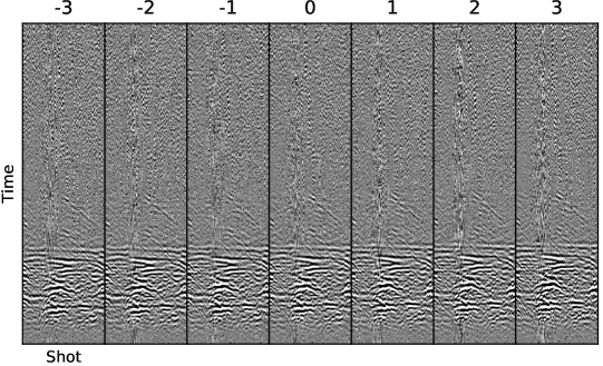
Figure 1: Three adjacent common offset gathers on either side of a central gather exhibit the redundant information contained in higher dimensions of seismic data.

Finally, several previous proposals were only trained using one dataset. As a result, the network will not have been exposed to all of the variations it may encounter in seismic data, and so its behavior on other datasets is unpredictable. Training using a diverse range of datasets allows the network to experience a wide range of situations and so reduce the risk of overfitting.

Our hypothesis is that a U-net, based on a pretrained ResNet, and provided with information from multiple adjacent gathers, will produce an effective tool for denoising seismic data. Applied to blended data in a gather dimension in which the blending noise is incoherent, it may also be used for deblending. By training it on a diverse training dataset, we believe it will exhibit the ability to generalize well to other datasets not used during training.

2 Materials and Methods

2.1 Network Architecture

We use a U-net model (Ronneberger et al., 2015), with a ResNet34 architecture as the encoder (He et al., 2016), using the implementation in Fast.ai version 1.0.53. The channel dimension is used to provide adjacent common offset gathers as input. ResNet34 expects three input channels. Thus, when the number of adjacent common offset gathers provided on either side of the gather being denoised is not one, we modify the first convolutional layer to have the appropriate kernel shape.

2.2 Training

We train the network using synthetic data, which we generate with an acoustic propagator and twenty randomly generated wave speed models. A slice through one of these models is shown in Figure 2. To ensure that the network behaves robustly on unseen data, these wave speed models exhibit more extreme variability than is generally found in reality. We use a Ricker wavelet source with a peak frequency of 35 Hz and a source and receiver spacing of 5 m. Each model is used to create one dataset with 300 towed receivers and 250 shots, with a shot record length of 1.2 s and a time sample interval of 0.001 s. The data are synthetically blended. This is achieved by creating a continuous recording for each dataset, where the shot records from the dataset are added with a time delay between shots. The average time delay and the jitter in the time delay are randomly chosen for each dataset between 0.5 and 1.5 s, and between 0.1 and 0.6 s, respectively. As this time delay is sometimes shorter than the shot record length, the shots may overlap. We then extract overlapping sections of this record corresponding to each shot record, including the blending noise. To increase the ability of the model to recognize other forms of noise, we also add data from real datasets to the synthetic data. This not only adds realistic noise, such as cable and swell noise, but, since the real datasets also contain signal, simulates interference from other nearby surveys. The datasets used are field data from cruises Rolling Deck To Repository (2015b), Rolling Deck To Repository (2015c), and Rolling Deck To Repository (2015d). White Gaussian noise is also added. Example common offset gathers of the input and target synthetic data are shown in Figure 3. Data from two of the wave speed models are reserved for use as a validation dataset.

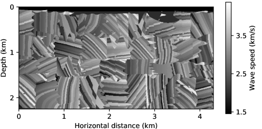
Figure 2: A vertical slice through one of the synthetic models used to generate training data.

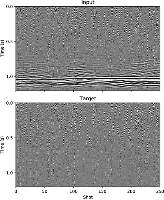
Figure 3: An example noisy common offset gather and the corresponding noise that are used as the input and target during training.

We initialize the ResNet portion of the model using pretrained weights. These are the weights obtained by training on the ImageNet dataset. We use the default version of these weights distributed with PyTorch (Paszke et al., 2017). As these weights are designed for three input channels (the red, green, and blue channels of ImageNet images), we replace the weights in the first convolution with the sum of the pretrained weights in the channel dimension, divided by the new number of input channels, repeated for each new input channel:

$$W_{c,x,y}=\frac{\sum_{i=1}^{3}W^{p}_{i,x,y}}{N},$$ (1)

where $W$ are the weights used in the first convolutional layer of the network, $W^{p}$ are the corresponding pretrained weights, $c$, $x$, and $y$ are the channel, vertical, and horizontal indices, respectively, and $N$ is the new number of input channels. The remaining weights in the network (i.e., those not in the ResNet portion) are randomly initialized.

During training, the noisy data are the inputs, and the corresponding noise (the input minus the signal) is the target. We divide each input and target gather by the standard deviation of the input gather. As the pretrained ResNet weights expect the input to have 224 pixels in both height and width, we randomly extract squares of this size from the data. One such square is extracted from each common offset gather in the dataset per epoch. To further increase the range of inputs that the model is exposed to during training, we apply transformations to the data. These convolve the data in time with a random kernel (simulating the use of different source wavelets), randomly set the stride in the time dimension between one and five (altering the apparent frequency of the data), and randomly choose the stride used to select the adjacent common offset gathers between one and four (exposing the model to different receiver spacings).

We use the 1cycle training method (Smith, 2018) and the AdamW optimizer (Loshchilov and Hutter, 2017), with the mean squared error loss function. We initially only train the weights in the model that were randomly initialized, leaving the pretrained weights fixed. We use a learning rate of 0.01 for five epochs. We then train all of the weights for 350 epochs, using Fast.ai’s discriminative learning rate that increases from $1\times 10^{-6}$ to $1\times 10^{-3}$ with increasing depth in the model. A batch size of 32 is used throughout training.

2.3 Test Datasets

To test the trained model on a variety of inputs, we select four 2D marine streamer datasets from different regions of the world. These are the North Sea, Venezuela, Norway, and New Zealand (Mobil AVO Viking Graben Line 12, and cruises EW0404 (Rolling Deck To Repository, 2015f), EW0307 (Rolling Deck To Repository, 2015e), and EW0001 (Rolling Deck To Repository, 2015a), respectively).

As none of these datasets use blended acquisition, we synthetically blend the data from the North Sea, using the blending procedure described above, with a time delay between shots of $1.8\pm 0.2$ s.

To create a common mid-point (CMP) stack image using the North Sea data, we sort the data into CMP gathers, apply normal moveout (NMO) correction, and stack. We use an NMO velocity profile that is constant at 1500 m/s up to 0.5 s, rises to 2000 m/s at 2 s and then remains constant.

The model operates on patches of data with 224 pixels on each side. To apply it to a whole gather, we divide the gather into overlapping patches, apply the model to each, and use the mean value in the overlapping regions. We use a stride of 56 pixels in both time and shot dimensions.

3 Results

3.1 Number of adjacent common offset gathers in input

We train the network using, as additional channels in the input, varying numbers of adjacent common offset gathers on both sides of the gather that corresponds to the target. Each configuration is trained using the training procedure described above, but with only 10 epochs in the second training stage. The training is repeated 45 times for each configuration, with different random initializations, and the minimum mean squared error loss achieved on the validation dataset is recorded.

The results, displayed in Figure 4, show that the loss decreases rapidly from 0 to 1 adjacent gathers, indicating that the model uses the information contained in these additional channels effectively. The loss continues to decrease up to 3 adjacent gathers, before increasing slightly and then remaining almost constant up to 8 adjacent gathers.

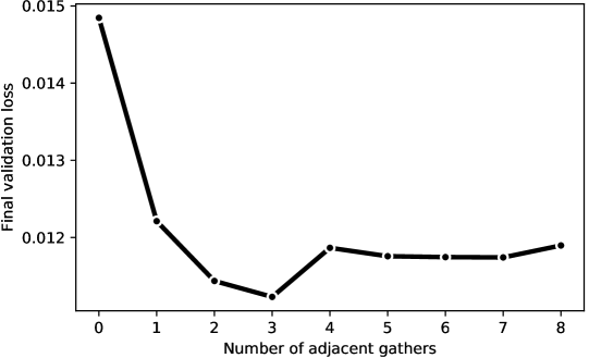
Figure 4: The best results are obtained when three adjacent common offset gathers on both sides of the gather being denoised are provided in the input.

Subsequent results use 3 adjacent gathers.

3.2 Deblending

We apply the trained network to the blended North Sea data. Figure 5 shows the result on one common offset gather. We calculate the mean signal-to-noise ratio using

$$\text{SNR}(data)=\frac{1}{n_{s}}\sum_{s=1}^{n_{s}}10\log_{10}\left(\frac{||\mathit{signal}_{s}||^{2}_{2}}{||\mathit{signal}_{s}-\mathit{data}_{s}||^{2}_{2}}\right),$$ (2)

where $\mathit{signal}$ is the unblended dataset, $s$ is the shot index, and $n_{s}$ is the number of shots in the dataset. Using this metric, the SNR of the input data is -3.6 dB, while that of the output deblended data is 16.5 dB. This is comparable with improvements in SNR reported using other techniques on different datasets, such as Chen et al. (2018) reporting an increase in SNR from 1.62 dB to 16.55 dB, and Zu et al. (2018) reporting an increase from 0 dB to 19.18 dB.

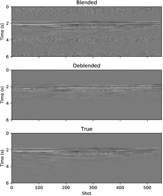
Figure 5: Common offset gathers before (input) and after deblending, and the unblended data.

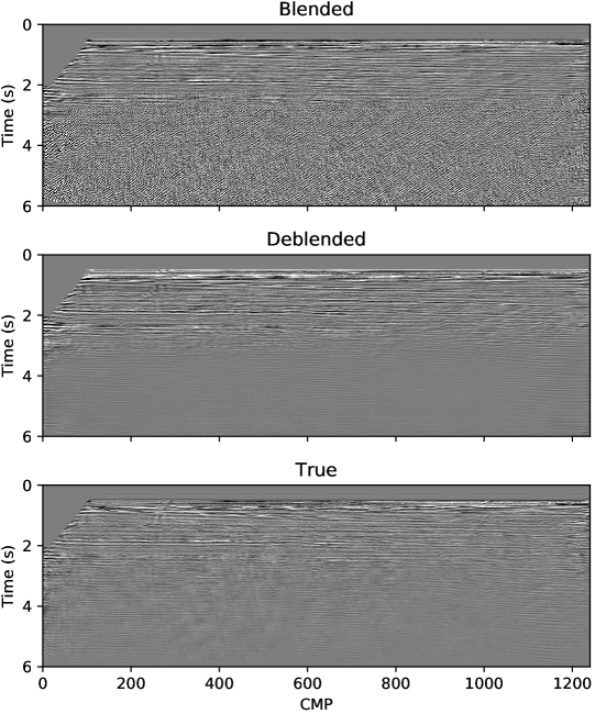
Figure 6: CMP stack images produced using the North Sea data, before (input) and after deblending, and using the unblended data. Deblending removes the blending noise artifacts. The underlying signal is reduced, but still visible.

We create CMP stack images to produce the result shown in Figure 6. The blending artifacts are less severe in the output.

3.3 Noise removal

When we apply the model, without any modification, to three noisy datasets from different parts of the world, we obtain the results shown in Figure 7. The model effectively removes the noise. Some signal is also visible in the estimated noise.

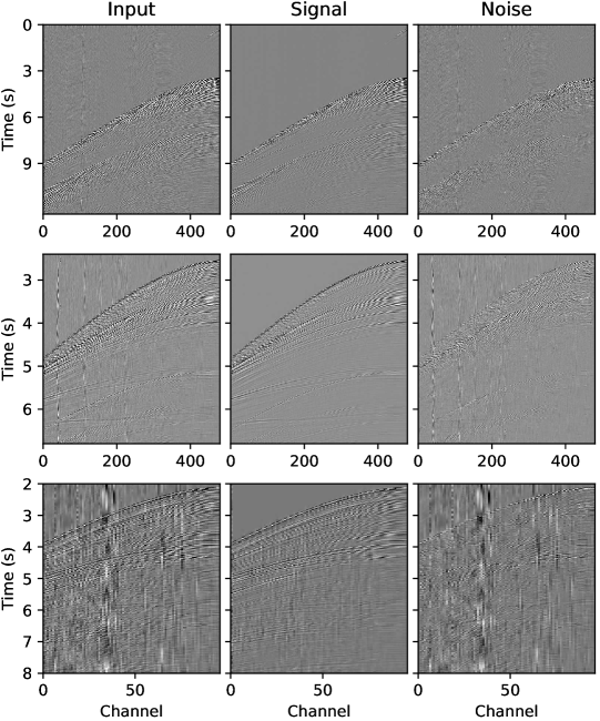
Figure 7: Noise removal from marine data acquired in Venezuela, Norway, and New Zealand. The output of the network, the estimated noise, is shown on the right, while the estimated signal, shown in the center, is obtained by subtracting the estimated noise from the input. The majority of the noise is removed, but some signal is also lost.

4 Discussion

Increasing loss with number of adjacent gathers

In theory, the loss should not increase as the number of adjacent gathers provided as input to the model increases, as the model may disregard the additional gathers if they do not provide useful information. It is possible that the loss increases in our experiment when more than three adjacent gathers are provided as beyond this point the useful information provided by additional gathers is not sufficient to compensate for the larger number of training epochs that will be required due to the increasing number of weights that need to be trained.

Alternative adjacent gathers

We use adjacent common offset gathers as the additional input channels provided to the network. Alternatives include constructing the additional input channels so that slices of the input in the channel dimension correspond to NMO corrected CMP gathers. In this setup, the blending noise is incoherent in two dimensions of the input, while the signal should be coherent and relatively flat. This may aid the network to remove the blending noise, but results in higher computational cost, and also requires a velocity model to perform the NMO correction.

Signal loss

The apparent signal leakage into the estimated noise, visible when the model is applied to real datasets, is undesirable. Inspection of the results suggests that small variations in amplitude are being identified by the model as noise. This is likely to be due to the model being trained using synthetic data, where such variations are not present. Incorporation of some real data into the training dataset may help to reduce this effect.

Application to land data

Denoising methods that rely on identifying signal by its coherency are less reliable for seismic data acquired on land. This is because static shifts, caused by near-surface variations, and irregular acquisition spacing due to obstacles, may cause the signal to also be incoherent across traces. Applying static corrections and interpolation to regularize the acquisition geometry may thus be necessary before attempting to attenuate the noise.

Black box method

Deep learning-based methods may be regarded as a black box, where it is not possible to explain why particular results were produced or to predict how the methods will respond to new inputs. The compensation for this sacrifice is that the methods are capable of more sophisticated operations than we are able to express in mathematically derived approaches. A median filter is easily understood, but will struggle when the underlying signal is not well approximated by a line and when there are crossing events. In contrast, a neural network can, in theory, learn to recognize these situations and handle them appropriately.

5 Conclusion

After being trained once, the method denoised and deblended datasets from different parts of the world that it had not seen previously, with moderate accuracy. The method removed noise effectively, but also removed some signal. The hypothesis is therefore validated for situations where the speed of the method is more important than preserving all of the signal, such as during fast-track processing and quality control.

References

- Baardman et al. (2019) Rolf Baardman, Constantine Tsingas, et al. Classification and suppression of blending noise using convolutional neural networks. In SPE Middle East Oil and Gas Show and Conference. Society of Petroleum Engineers, 2019.
- Chen et al. (2018) Yangkang Chen, Shaohuan Zu, Yufeng Wang, and Xiaohong Chen. Deblending of simultaneous source data using a structure-oriented space-varying median filter. Geophysical Journal International, 216(2):1214–1232, 2018.
- Claus and van Gemert (2019) Michele Claus and Jan van Gemert. Videnn: Deep blind video denoising. In Proceedings of the IEEE Conference on Computer Vision and Pattern Recognition Workshops, pages 0–0, 2019.
- Gulunay (1986) Necati Gulunay. FXDECON and complex Wiener prediction filter. In SEG Technical Program Expanded Abstracts 1986, pages 279–281. Society of Exploration Geophysicists, 1986.
- He et al. (2016) Kaiming He, Xiangyu Zhang, Shaoqing Ren, and Jian Sun. Deep residual learning for image recognition. In Proceedings of the IEEE conference on computer vision and pattern recognition, pages 770–778, 2016.
- Huo et al. (2012) Shoudong Huo, Yi Luo, and Panos G Kelamis. Simultaneous sources separation via multidirectional vector-median filtering. Geophysics, 77(4):V123–V131, 2012.
- Jin et al. (2018) Yuchen Jin, Xuqing Wu, Jiefu Chen, Zhu Han, and Wenyi Hu. Seismic data denoising by deep-residual networks. In SEG Technical Program Expanded Abstracts 2018, pages 4593–4597. Society of Exploration Geophysicists, 2018.
- Liu et al. (2018) Dawei Liu, Wei Wang, Wenchao Chen, Xiaokai Wang, Yanhui Zhou, and Zhensheng Shi. Random noise suppression in seismic data: What can deep learning do? In SEG Technical Program Expanded Abstracts 2018, pages 2016–2020. Society of Exploration Geophysicists, 2018.
- Liu et al. (2008) Yang Liu, Cai Liu, and Dian Wang. A 1d time-varying median filter for seismic random, spike-like noise elimination. Geophysics, 74(1):V17–V24, 2008.
- Loshchilov and Hutter (2017) Ilya Loshchilov and Frank Hutter. Fixing weight decay regularization in adam. arXiv preprint arXiv:1711.05101, 2017.
- Mandelli et al. (2019) Sara Mandelli, Vincenzo Lipari, Paolo Bestagini, and Stefano Tubaro. Interpolation and denoising of seismic data using convolutional neural networks. arXiv preprint arXiv:1901.07927, 2019.
- Moore et al. (2008) Ian Moore, Bill Dragoset, Tor Ommundsen, David Wilson, Camille Ward, and Daniel Eke. Simultaneous source separation using dithered sources. In SEG Technical Program Expanded Abstracts 2008, pages 2806–2810. Society of Exploration Geophysicists, 2008.
- Paszke et al. (2017) Adam Paszke, Sam Gross, Soumith Chintala, Gregory Chanan, Edward Yang, Zachary DeVito, Zeming Lin, Alban Desmaison, Luca Antiga, and Adam Lerer. Automatic differentiation in PyTorch. In NIPS Autodiff Workshop, 2017.
- Rolling Deck To Repository (2015a) Rolling Deck To Repository. Cruise EW0001 on RV Maurice Ewing, 2015a. URL http://www.rvdata.us/catalog/EW0001.
- Rolling Deck To Repository (2015b) Rolling Deck To Repository. Cruise EW0007 on RV Maurice Ewing, 2015b. URL http://www.rvdata.us/catalog/EW0007.
- Rolling Deck To Repository (2015c) Rolling Deck To Repository. Cruise EW0207 on RV Maurice Ewing, 2015c. URL http://www.rvdata.us/catalog/EW0207.
- Rolling Deck To Repository (2015d) Rolling Deck To Repository. Cruise EW0210 on RV Maurice Ewing, 2015d. URL http://www.rvdata.us/catalog/EW0210.
- Rolling Deck To Repository (2015e) Rolling Deck To Repository. Cruise EW0307 on RV Maurice Ewing, 2015e. URL http://www.rvdata.us/catalog/EW0307.
- Rolling Deck To Repository (2015f) Rolling Deck To Repository. Cruise EW0404 on RV Maurice Ewing, 2015f. URL http://www.rvdata.us/catalog/EW0404.
- Ronneberger et al. (2015) Olaf Ronneberger, Philipp Fischer, and Thomas Brox. U-net: Convolutional networks for biomedical image segmentation. In International Conference on Medical image computing and computer-assisted intervention, pages 234–241. Springer, 2015.
- Russakovsky et al. (2015) Olga Russakovsky, Jia Deng, Hao Su, Jonathan Krause, Sanjeev Satheesh, Sean Ma, Zhiheng Huang, Andrej Karpathy, Aditya Khosla, Michael Bernstein, et al. Imagenet large scale visual recognition challenge. International journal of computer vision, 115(3):211–252, 2015.
- Simonyan and Zisserman (2014) Karen Simonyan and Andrew Zisserman. Very deep convolutional networks for large-scale image recognition. arXiv preprint arXiv:1409.1556, 2014.
- Slang et al. (2019) Sigmund Slang, Jing Sun, Thomas Elboth, Steven McDonald, and Leiv-J. Gelius. Using convolutional neural networks for denoising and deblending of marine seismic data. In 81st EAGE Conference and Exhibition 2019, 2019.
- Smith (2018) Leslie N Smith. A disciplined approach to neural network hyper-parameters: Part 1–learning rate, batch size, momentum, and weight decay. arXiv preprint arXiv:1803.09820, 2018.
- Yosinski et al. (2014) Jason Yosinski, Jeff Clune, Yoshua Bengio, and Hod Lipson. How transferable are features in deep neural networks? In Advances in neural information processing systems, pages 3320–3328, 2014.
- Yu et al. (2018) Siwei Yu, Jianwei Ma, and Wenlong Wang. Deep learning tutorial for denoising. arXiv preprint arXiv:1810.11614, 2018.
- Zhang et al. (2017) Kai Zhang, Wangmeng Zuo, Yunjin Chen, Deyu Meng, and Lei Zhang. Beyond a gaussian denoiser: Residual learning of deep cnn for image denoising. IEEE Transactions on Image Processing, 26(7):3142–3155, 2017.
- Zhang et al. (2019) Mi Zhang, Yang Liu, Min Bai, Yangkang Chen, and Yuxi Zhang. Random noise attenuation using deep convolutional autoencoder. In 81st EAGE Conference and Exhibition 2019, 2019.
- Zu et al. (2018) Shaohuan Zu, Hui Zhou, Rushan Wu, Weijian Mao, and Yangkang Chen. Hybrid-sparsity constrained dictionary learning for iterative deblending of extremely noisy simultaneous-source data. IEEE Transactions on Geoscience and Remote Sensing, 2018.