Integrated Nested Laplace Approximations (INLA)

Abstract

This is a short description and basic introduction to the Integrated nested Laplace approximations (INLA) approach. INLA is a deterministic paradigm for Bayesian inference in latent Gaussian models (LGMs) introduced in Rue et al., ²⁷. INLA relies on a combination of analytical approximations and efficient numerical integration schemes to achieve highly accurate deterministic approximations to posterior quantities of interest. The main benefit of using INLA instead of Markov chain Monte Carlo (MCMC) techniques for LGMs is computational; INLA is fast even for large, complex models. Moreover, being a deterministic algorithm, INLA does not suffer from slow convergence and poor mixing. INLA is implemented in the R package R-INLA, which represents a user-friendly and versatile tool for doing Bayesian inference. R-INLA returns posterior marginals for all model parameters and the corresponding posterior summary information. Model choice criteria as well as predictive diagnostics are directly available. Here, we outline the theory behind INLA, present the R-INLA package and describe new developments of combining INLA with MCMC for models that are not possible to fit with R-INLA.

Keywords: Approximate Bayesian inference, INLA, Laplace approximation, Latent Gaussian model.

1 Where can INLA be applied

Latent Gaussian Models (LGM) are the class of Bayesian models amenable to INLA-based inference. An LGM consists of three elements: a likelihood model, a latent Gaussian field and a vector of hyperparameters. The data $\bm{y}$ are assumed to be conditionally independent given the latent Gaussian field $\bm{x}$ so that the univariate likelihood model describes the marginal distribution of the observation. As in the generalized linear model framework, the mean, or another measure of central tendency, of the observation $y_{i}$ is linked to a Gaussian linear predictor $\eta_{i}$ through a known link function. The linear predictor is then additive with respect to other effects:

$$\eta_{i}=\mu+\sum_{j}\beta_{j}z_{ij}+\sum_{k}w_{k}\ f^{k}(u_{ik})$$ (1)

Here $\mu$ is an overall intercept, $\bm{z}$ are known covariates with linear effect $\bm{\beta}$ and $\bm{w}$ a vector of known weights. The terms $\bm{f}^{k}$ are used to model random effects of the covariate $\bm{u}$. In the INLA framework we assign $\mu$, $\bm{\beta}$ and $\bm{f}^{k}$, $k=1,\dots,K$ a Gaussian prior. The latent Gaussian field is then $\bm{x}=\{\bm{\eta},\mu,\bm{\beta},\bm{f}^{1},\bm{f}^{2},\dots\}$. Note that we include the linear predictor in the latent field. This is mainly due to the fact having each data point $y_{i}$ dependent on the latent Gaussian field only through one single element of $\bm{x}$, namely $\eta_{i}$ greatly simplifies the computations needed in the INLA algorithm, see for example Rue et al., ²⁷ and Rue et al., ²⁸ for details. For this reason, a small random noise term where the precision parameter is fixed to a high value is always automatically added to the model.

The hyperparameters $\bm{\theta}$ can appear in the likelihood model (for example the variance in the Gaussian likelihood or the shape parameter in the Gamma one) or/and in the latent field, typically as dispersion parameters, spatial correlation parameters or autoregression coefficients in the $\bm{f}^{k}$ terms. Formally the model can be written as:

$$\bm{y}|\bm{x},\bm{\theta} \sim\prod\pi(y_{i}|\eta_{i},\bm{\theta})$$

$$\bm{x}|\bm{\theta} \sim\mathcal{N}(\bm{0},\bm{Q}^{-1}(\bm{\theta}))$$

$$\bm{\theta} \sim\pi(\bm{\theta})$$

where $\bm{Q}(\bm{\theta})$ is the precision (inverse of the covariance) matrix of the latent Gaussian field. A limitation of the INLA approach is the size of the hyperparameter vector $\bm{\theta}$. While $\bm{y}$ and $\bm{x}$ can be large, $\bm{\theta}$ should be small, say $<15$. This is due to the numerical integration that has to be carried over the $\bm{\theta}$ space. The dependence structure of the data is mainly captured by the precision matrix $\bm{Q}(\bm{\theta})$ through a clever choice of the terms $\bm{f}^{k}$ in (1). In order for INLA to perform efficiently, we require the precision matrix $\bm{Q}(\bm{\theta})$ to be sparse.

Many of the models that are commonly used as prior for the $\bm{f}^{k}$ terms belong to the class of so called Gaussian Markov Random field (GMRF). GMRFs can be used to model smooth effects of a covariate, random effects, measurement errors, temporal dependencies, and so on (see Rue and Held, ²⁶). When it comes to spatial dependence, there exist GMRF models for areal data, such as the CAR or BYM model proposed by Besag et al., ³. Continuous spatial dependence can be specified using the so-called SPDE approach ²⁰, ² which creates an approximated GMRF representation of the Matérn covariance field based on stochastic partial differentiation equations. GMRFs are Gaussian models endowed with Markov properties. These, in turn, are linked to the non-zero structure of the precision matrix in the sense that, if two elements of the field are conditionally independent given all the others, then the corresponding entry of the precision matrix is equal to zero, see Rue and Held, ²⁶. In practice, choosing GMRF priors for $\bm{f}^{k}$, induces sparsity in the precision matrix $\bm{Q}(\bm{\theta})$.

The resulting posterior density of $\bm{x}$ and $\bm{\theta}$ given $\bm{y}$ is:

$$\pi(\bm{x},\bm{\theta}|\bm{y})\propto\exp\left(-\frac{1}{2}\bm{x}^{T}\bm{Q}(\bm{\theta})\bm{x}+\sum_{i}\log(\pi(y_{i}|\eta_{i},\bm{\theta}))+\log\pi(\bm{\theta})\right)$$ (2)

This is a high dimensional density that is difficult to interpret. Often the main interest lies in the marginal posterior of the latent field $\pi(x_{i}|\bm{y})$ or of the hyperparameters $\pi(\theta_{j}|\bm{y})$. INLA provides an approximation to such marginal posterior densities, which can then be used to compute approximated summary statistics of interest such as posterior means, variances or quantiles.

To sum up, INLA can be applied to LGMs which fulfill the following assumptions:

1. Each data point depends on only one of the elements in the latent Gaussian field $\bm{x}$, the linear predictor, so that the likelihood can be written as:

   $$\bm{y}|\bm{x},\bm{\theta}\sim\prod_{i}\pi(y_{i}|\eta_{i},\bm{\theta}).$$

2. The size of the hyperparameter vector $\bm{\theta}$ is small (say $<15$)

3. The latent field $\bm{x}$, can be large but it is endowed with some conditional independence (Markov) properties so that the precision matrix $Q(\bm{\theta})$ is sparse.

4. The linear predictor depends linearly on the unknown smooth function of covariates.

5. The inferential interest lies in the univariate posterior marginals $\pi(x_{i}|\bm{y})$ and $\pi(\theta_{j}|\bm{y})$ rather than in the joint posterior $\pi(\bm{x},\bm{\theta}|\bm{y})$.

There are some, rather extreme, cases of LGM where the use of INLA has been seen as problematic ⁹, ³⁰. If the likelihood is binomial or Poisson, inaccuracies can occur with low counts and low degree of smoothing. Variances of both random and fixed effects tend to be underestimated by INLA while means are usually well estimated. Ferkingstad and Rue, ⁹ introduce a correction, implemented in the R-INLA package, that, at a negligible computational cost, alleviates the problem.

2 The INLA computing scheme

The INLA framework provides deterministic approximations to the univariate posterior marginals for the hyperparameters $\pi(\theta_{j}|\bm{y})$ and the latent field $\pi(x_{i}|\bm{y})$. Thus, interest lies in:

$$\pi(\theta_{j}|\bm{y}) =\int\int\pi(\bm{x},\bm{\theta}|\bm{x})d\bm{x}\ d\bm{\theta}_{-j}=\int\pi(\bm{\theta}|\bm{y})\ d\bm{\theta}_{j}$$ (3)

$$\pi(x_{i}|\bm{y}) =\int\int\pi(\bm{x},\bm{\theta}|\bm{x})d\bm{x}_{-i}\ d\bm{\theta}=\int\pi(x_{i}|\bm{\theta},\bm{y})\pi(\bm{\theta}|\bm{y})\ d\bm{\theta}$$ (4)

Notice that, because of the model requirements explained in Section 1 the integral with respect to $\bm{x}$ in (3) and (4) can be (and usually is) highly multidimensional, while the integral with respect to $\bm{\theta}$ is only moderate in size and can be solved via some numerical integration scheme. The core of the INLA methodology lies therefore in building clever approximations to the posterior for the hyperparameters $\pi(\bm{\theta}|\bm{y})$ and the full-conditional density $\pi(x_{i}|\bm{\theta},\bm{y})$ that allow to avoid the cumbersome integration with

An approximation to $\pi(\bm{\theta}|\bm{y})$ is built starting from the identity:

$$\pi(\bm{\theta}|\bm{y})=\frac{\pi(\bm{x},\bm{\theta}|\bm{y})}{\pi(\bm{x}|\bm{\theta},\bm{y})}\propto\frac{\pi(\bm{y}|\bm{x},\bm{\theta})\pi(\bm{x}|\bm{\theta})\pi(\bm{\theta})}{\pi(\bm{x}|\bm{\theta},\bm{y})}$$ (5)

Notice that, while the numerator in (5) is easy to compute, the denominator is, in general, not available in closed form and hard to compute. INLA approximates (5) at a specific value $\bm{\theta}^{k}$ of the hyperparameters vector as:

$$\widetilde{\pi}(\bm{\theta}^{k}|\bm{y})\propto\frac{\pi(\bm{y}|\bm{x},\bm{\theta}^{k})\pi(\bm{x}|\bm{\theta}^{k})\pi(\bm{\theta}^{k})}{\widetilde{\pi}_{G}(\bm{x}|\bm{\theta}^{k},\bm{y})}$$ (6)

where $\widetilde{\pi}_{G}(\bm{x}|\bm{\theta}^{k},\bm{y})$ is a Gaussian approximation to the full conditional $\bm{x}|\bm{\theta}^{k},\bm{y}$ build by matching the mode and the curvature at the mode. This expression is equivalent to Tierney and Kadane, ³³’s Laplace approximation of a marginal posterior distribution. The computationally expensive part of evaluating (6) is the Cholesky decomposition of the $Q(\bm{\theta}^{k})$ matrix necessary to evaluate the denominator and that needs to be performed for each value $\bm{\theta}^{k}$. Here, the sparseness of the precision matrix is essential, see Rue et al., ²⁷ for more details.

Next, we need to find an approximation $\widetilde{\pi}(x_{i}|\bm{\theta}^{k},\bm{y})$ of $x_{i}|\bm{\theta}^{k},\bm{y}$. This step is more involved as it has to be repeated for each element of the, virtually very large dimensional, vector $\bm{x}$. One could use the marginal from the Gaussian approximation $\widetilde{\pi}_{G}(\bm{x}|\bm{\theta}^{k},\bm{y})$ from 6. While this is very fast, it is usually not very accurate. As an alternative, we can start by writing $\pi(x_{i}|\bm{\theta}^{k},\bm{y})$ as

$$\pi(x_{i}|\bm{\theta}^{k},\bm{y})=\frac{\pi(\bm{x}|\bm{\theta},\bm{y})}{\pi(\bm{x}_{-i}|x_{i},\bm{\theta},\bm{y})}\propto\frac{\pi(\bm{y}|\bm{x},\bm{\theta})\pi(\bm{x}|\bm{\theta})\pi(\bm{\theta})}{\pi(\bm{x}_{-i}|x_{i},\bm{\theta},\bm{y})}$$ (7)

where $\bm{x}_{-i}$ indicates the vector $\bm{x}$ without the $i^{\text{th}}$ element. This expression is similar to 5. An approximation to $\pi(x_{i}|\bm{\theta}^{k},\bm{y})$ can then be constructed by approximating the denominator in (7) by matching the mode and the curvature at the mode. This is again equivalent to Tierney and Kadane, ³³’s Laplace approximation. The problem with (5) is that it is very computationally demanding as it requires factorizing many times a large precision matrix. Rue et al., ²⁷ propose therefore a third approximation, denoted the Simplified Laplace approximation, which corrects the Gaussian approximation for location and skewness by a Taylor’s series expansion around the mode of the Laplace approximation. All three approximations are available in the R-INLA package. The Simplified Laplace is the default choice.

The last step is the numerical integration scheme to solve the integral with respect to $\bm{\theta}$ in (3) and 4. The R-INLA package offers three possible alternatives. The first is to build a grid on the $\bm{\theta}$ space around the mode of $\widetilde{\pi}(\bm{\theta}|\bm{y})$ (int.strategy=’grid’). This strategy gives the most accurate approximations but the number of points in the grid grows exponentially with the size of the $\bm{\theta}$ vector. It is the default choice in the R-INLA package if the dimension of $\bm{\theta}$ is one or two. The second strategy is to use a so called central composite design to cleverly locate fewer points around the mode of $\widetilde{\pi}(\bm{\theta}|\bm{y})$ (int.strategy=’ccd’). This is the default strategy for dimensions of $\bm{\theta}$ larger than two. Finally one can ignore the variability of the hyperparameter and just use the mode of $\widetilde{\pi}(\bm{\theta}|\bm{y})$ (int.strategy=’eb’).

Putting all together, the INLA computing scheme is as follows:

1. Explore the $\bm{\theta}$ space through the approximation $\widetilde{\pi}(\bm{\theta}|\bm{y})$. Find the mode of $\widetilde{\pi}(\bm{\theta}|\bm{y})$ and locate a series of points $\{\bm{\theta}^{1},\dots,\bm{\theta}^{K}\}$ in the area of high density of $\widetilde{\pi}(\bm{\theta}|\bm{y})$.

2. For the $K$ selected support points compute $\widetilde{\pi}(\bm{\theta}^{1}|\bm{y}),\ldots,\widetilde{\pi}(\bm{\theta}^{K}|\bm{y})$ using (6).

3. For each selected $\bm{\theta}^{k}$ point, approximate the density of $x_{i}|\bm{\theta},\bm{y}$ as $\widetilde{\pi}(x_{i}|\bm{\theta}^{k},\bm{y})$ for $k=1,\dots,K$ using one of the three possible approximations: Laplace, Simplified Laplace or Gaussian.

4. Solve (4) via numerical integration as:

   $$\widetilde{\pi}(x_{i}|\bm{y})=\sum_{k=1}^{K}\widetilde{\pi}(x_{i}|\bm{\theta}^{k},\bm{y})\widetilde{\pi}(\bm{\theta}^{k}|\bm{y})\Delta_{k}$$ (8)

   Where $\Delta_{k}$ are appropriate weights, which would be equal to 1 for example if all support points would be equi-distantly chosen. The integral (3) can be solved similarly.

The scheme above sheds light on the name INLA: the nested Laplace approximations are those performed in steps 2 and 3 while the integrated bit comes from the numerical integration in step 4.

Note that the error committed in (8) comes from two different sources: one is the approximation error due to approximating $\pi(x_{i}|\bm{\theta}^{k},\bm{y})$ with $\widetilde{\pi}(x_{i}|\bm{\theta}^{k},\bm{y})$, the other is due to the numerical integration scheme and the choice of the support points $\bm{\theta}^{k}$. Using a Gaussian likelihood, the full conditional $\pi(\bm{x}|\bm{\theta},\bm{y})$ and (of course) its marginals $\pi(x_{i}|\bm{\theta},\bm{y})$ are also Gaussian. This implies that, for each value of $\bm{\theta}$, (5) can be computed exactly. The only source of error in (8) is then the numerical integration scheme. We will look in details at this special case in the Section 3.

An interesting feature of INLA is that it can approximate, as a bi-product of the main computations, leave-one-out cross-validatory model checks without re-running the model with individually removed observations. These include the conditional predictive ordinate (CPO) and probability integral transform (PIT) values that can be used to asses the quality of the model. See Held et al., ¹⁷ for details about how these measures are computed and a comparison with MCMC results. The R-INLA package returns an additional flag vector indicating when an observation-specific CPO values is not accurately approximated, and offers the user the helper function inla.cpo to replace this value with the correct value obtained by removing the corresponding observation from the data frame and refitting the model. INLA can also provide estimates for deviance information criterion (DIC) ³², Watanabe-Akaike information criterion (WAIC) ³⁵ and marginal likelihood. The marginal likelihood is a well established model selection criterion in Bayesian statistics and can be used for Bayesian model averaging. Recently Hubin and Storvik, ¹⁹ have studied the accuracy of the marginal likelihood estimate provided by INLA finding it very accurate.

3 The Gaussian Likelihood case

Assume we observe the time series shown as dots in Figure 1(a) and our goal is to recover the underlying smooth trend. Assume that, given the vector $\bm{\eta}=(\eta_{1},\dots,\eta_{T})$, the observations $y_{t}$ are independent and Gaussian distributed with mean $\eta_{t}$ and known unit variance:

$$y_{t}|\eta_{t}=\mathcal{N}(\eta_{t},1);\ t=1,\dots,T$$

The linear predictor $\eta_{t}$ is linked to a smooth effect of time $t$ as:

$$\eta_{t}=f(t)$$

Random walk models are a popular choice for modeling smooth effects of covariates or, as in this case, temporal effects (see for example chapter 3 in Rue and Held, ²⁶). Here, we choose a second order random walk model as prior distribution for the vector ${\bm{f}}=(f(1),\dots,f(T))$, so that:

$$\pi({\bm{f}}|\theta)\propto\theta^{(T-2)/2}\exp\left\{-\frac{\theta}{2}\sum_{t=3}^{T}[f(t)-2f(t-1)+f(t-2)]^{2}\right\}=\mathcal{N}(\bm{0},\mathbf{Q}({\theta})^{-1}).$$

Thus, ${\bm{f}}|\theta$ is Gaussian distributed with mean $\bm{0}$ and precision (inverse covariance) matrix $\mathbf{Q}({\theta})$. The precision parameter $\theta$ controls the smoothness of the vector $\bm{f}$. Note that the precision matrix $\mathbf{Q}(\theta)$ is a band matrix with bandwidth $2$ and therefore it is sparse. We complete the model by assigning $\theta$ a prior distribution. Here, we choose the newly proposed penalised complexity (PC) prior ³¹ with parameters $u=1$ and $\alpha=0.01$. This is equivalent to using an exponential prior with mean $-u/\log(\alpha)$ for the standard deviation parameter $1/\sqrt{\theta}$. The resulting model is an LGM that fulfills the requirements listed earlier, namely: each data point depends on only one element of the latent field, the precision matrix of the latent Gaussian field is sparse and we have only one hyperparameter. Our main inferential interest lies in the posterior marginal for the smooth effect $\pi(f(t)|\bm{y})$, $t=1,\dots,T$. We follow the scheme outlined in Section 2: After finding the mode of $\theta|\bm{y}$ via an optimization algorithm, we select support points $\{\theta^{1},\dots,\theta^{K}\}$ on a grid around the mode so that they represent the density mass. Then, we approximate $\pi(\bm{\theta}|\bm{y})$ for each value $\{\theta^{1},\dots,\theta^{K}\}$. In this special case the full conditional $\pi(\bm{x}|\bm{y},\bm{\theta})$ is Gaussian and therefore (5) can be computed, for any value of $\theta$, without the need to approximate the denominator. If we are interested in the posterior marginal for $\theta$ we can interpolate the points $\{\pi(\theta^{1}|\bm{y}),\dots,\pi(\theta^{K}|\bm{y})\}$ using, for example, a spline and normalize the density. Figure 1(b) shows the normalized density $\pi(\theta|\bm{y})$. On the x-axis ten selected support points $\theta^{1},\ldots,\theta^{10}$ are indicated. The density line is obtained by fitting a spline to $\{\theta^{k},\log(\pi(\theta^{k}|y)\}$ and then normalizing so that the density integrates to 1.

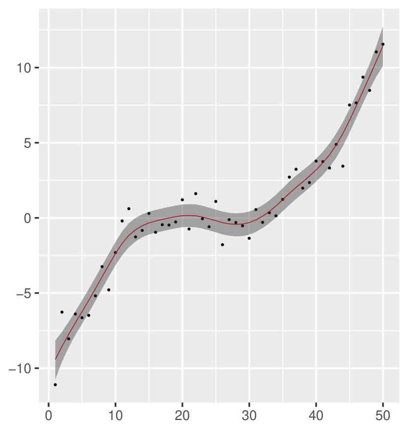
(a)

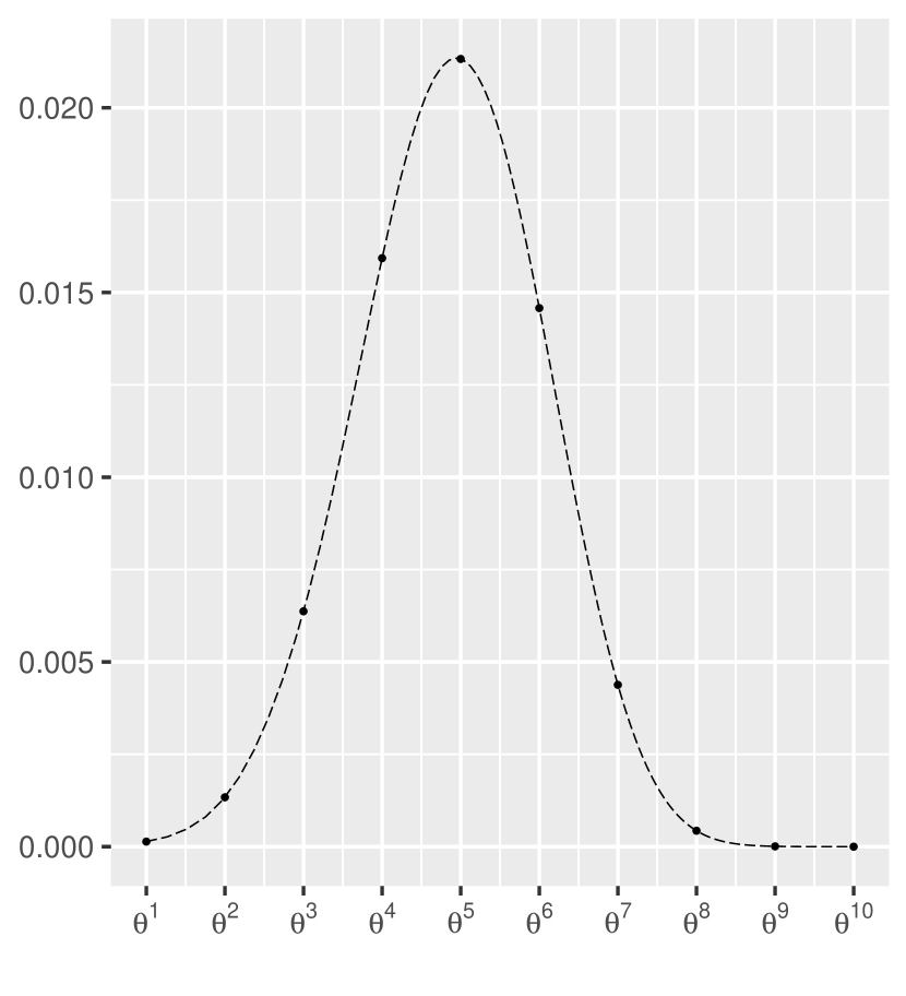
(b)

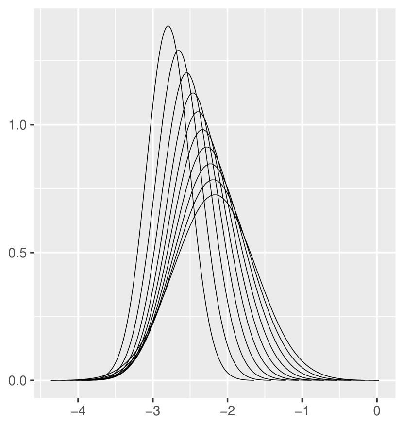
(c)

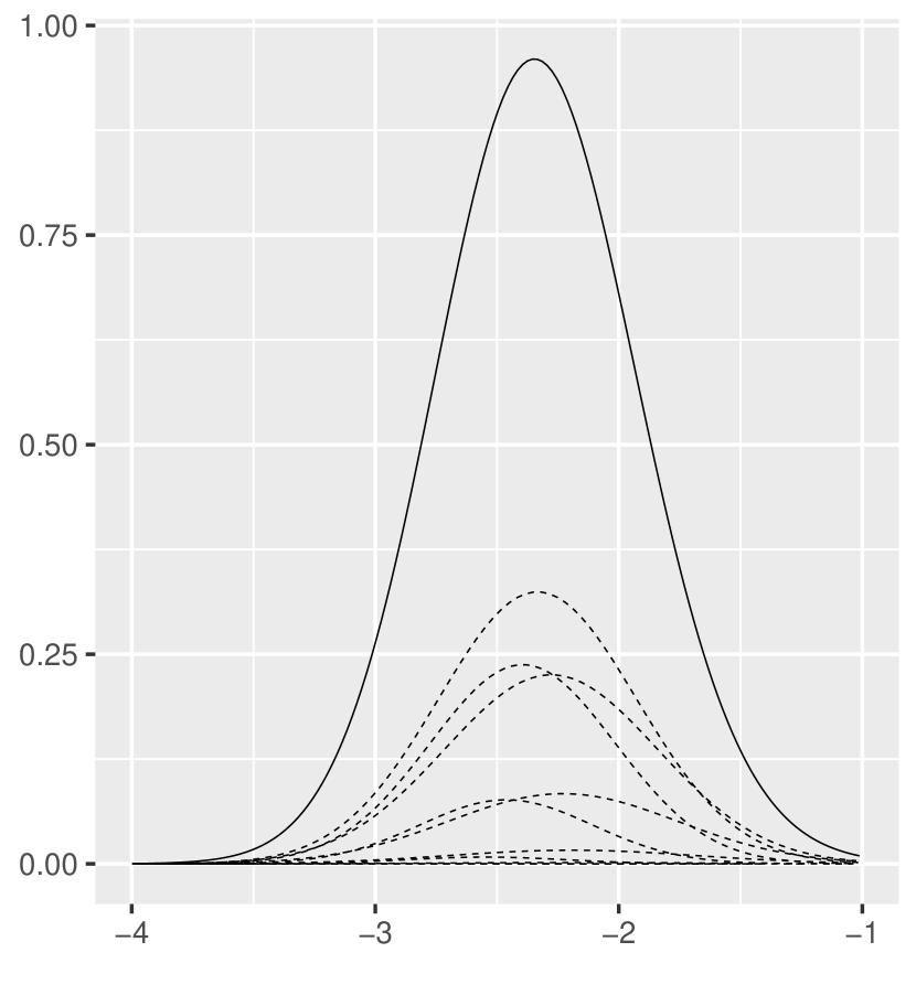
(d)

Figure 1: a) Observed time series (dots) together with the posterior estimated mean (black line). The grey band indicates a 95% pointwise credible interval around the estimated smooth curve. b) Posterior distribution for the hyperparameter $\pi(\theta|\bm{y})$. The black dotes indicate the density at the chosen points $\theta^{1},\dots,\theta^{K}$. c) unweighted full conditional densities $\pi(x_{10}|\bm{y},\theta^{k})$, $k=1,\dots,K$. d) Broken lines: full conditional densities $\pi(x_{10}|\bm{y},\theta^{k})$, weighed by $\pi(\theta^{k}|\bm{y})\Delta_{k}$, $k=1,\dots,K$. The solid line indicates the approximation $\tilde{\pi}(x_{10}|\bm{y})$ obtained by summing the weighted full conditional densities.

If we are interested in $\pi(x_{i}|\bm{y})$, the next task is to approximate $\pi(x_{i}|\theta^{k},\bm{y})$. Again, since the full conditional of $\pi(\bm{x}|\theta^{k},\bm{y})$ is Gaussian, its marginal distributions can be easily found. Finally we need to compute $\widetilde{\pi}(x_{i}|\bm{y})$ via (4). Note that in this special case, the integrand can be computed exactly for each value of $\theta$, the only approximation error comes from the numerical integration scheme in (8). In the Gaussian likelihood case the approximation $\widetilde{\pi}(x_{i}|\bm{y})$ is a mixture of Gaussian densities $\pi(x_{i}|\bm{y},\theta^{k})$ weighted by $\tilde{\pi}(\theta^{k}|\bm{y})\Delta_{k}$, $k=1,\dots,K$. Figure 1(c) shows the 10 elements of the mixture to approximate $\pi(x_{10}|\bm{y})$ unweighted, while Figure 1(d) shows the same elements but weighed. The sum of the densities in Figure 1(d) gives the approximated posterior marginal $\tilde{\pi}(x_{10}|\bm{y})$ also shown in Figure 1(d). The procedure is repeated for each element of the vector $\bm{x}$. These approximated densities can then be used to compute posterior summary measures of interest. As an example, Figure 1(a) shows the posterior mean and 95% credible intervals for the underlying smooth function.

4 Using the INLA framework in practice: The R-INLA package

The R-INLA package provides a user friendly implementation of the INLA methodology. It can be downloaded from www.r-inla.org together with the free-standing external INLA program.

The model definition in R-INLA is similar to several other R packages, for example the mgcv package to fit generalized additive models ³⁷. There are two essential steps: 1) Define the linear predictor through a formula object; 2) Complete the model definition and fit the model using the function inla(). The fitted model is returned as an inla object. The formula can include fixed effects and random effects. Non-linear terms and random effects are included in the formula using the f() function. The specification of different latent Gaussian models, hyperpriors and model fitting options is straightforward. Results include the posterior marginal distributions of the latent effects and hyperparameters, as well as summary statistics. Furthermore, posterior estimates of linear combinations or transformations of the latent field can be obtained ²¹. Model choice criteria such as the marginal likelihood, DIC ³², WAIC ³⁵, conditional predictive ordinates and the probability integral transform are also available. In R-INLA there is no function “predict” as for glm or lm. Predictions must be done as a part of the model fitting itself. As prediction can be regarded as fitting a model with missing data, we can simply set y[i] = NA for those “locations” we want to predict. Predictive distributions, which are often of interest, are however not returned directly. Instead the posterior marginals for random effects and the linear predictor at the missing locations are returned. Adding the observational noise to the fitted values leads to the predictive distributions.

In the following we use a simple example of Poisson regression to illustrate the R-INLA library. In Section 4.3 we illustrate how to obtain the predictive distribution for a missing observation.

4.1 Data preparation and model specification

The Salm ⁷ dataset will be used throughout this tutorial, the same dataset is presented in both the OpenBugs tutorial and on R-INLA example page on www.r-inla.org. The data concern the number of revertant colonies of TA98 Salmonella observed on each of three replicate plates tested at each of six dose levels of quinoline. A certain dose-response curve is suggested by theory and no effect of plate is assumed.

Let $y_{ij}$, $j=1,\dots,3$, $i=1,\dots,6$ denote the number of colonies found on plate $j$ for dose $i$ and let $x_{i}$ indicate the $i^{\text{th}}$ dose. We assume a Poisson likelihood and use a random effect to allow for over-dispersion:

$$y_{ij}\mid\lambda_{ij} \sim\text{Poisson}(\lambda_{ij}) i=1,\dots,6\ j=1,\dots,3$$

$$\log(\lambda_{ij}) =\beta_{0}+\beta_{1}\log(x_{i}+10)+\beta_{2}x_{i}+u_{ij}$$

Here, $\lambda_{ij}$ is the expected number of colonies at dose $i$ for plate $j$. Further, $\beta_{0}$ denotes the intercept, $\beta_{1}$ and $\beta_{2}$ fixed effects, and $u_{ij}\mid\sigma^{2}\sim\mathcal{N}(0,\sigma^{2})$ is a random effect accounting for unobserved heterogeneity. Putting this model in the LGMs framework described in Section 1, the latent Gaussian field is $\{\lambda_{11},\dots,\lambda_{36},\beta_{0},\beta_{1},\beta_{2},u_{11},\dots,u_{36}\}$. The model has one hyperparameter, namely the variance $\sigma^{2}$ of the random effect $\bm{u}$. To complete the model we need to define a prior distribution for $\sigma^{2}$. In the INLA world priors are usually not defined on variances but on its inverse, the precision parameters: here we use a PC-prior ³¹ with parameters $u=1$ and $\alpha=0.01$ as prior for the log precision $\log(\tau)=-2\log(\sigma)$.

The model is specified as follows as a formula object:

# load the data set
data(Salm)
# rename the columns to fit the notation
names(Salm) = c("y", "x", "u")
head(Salm)

##    y  x u
## 1 15  0 1
## 2 21  0 2
## 3 29  0 3
## 4 16 10 4
## 5 18 10 5
## 6 21 10 6

# specify the prior for the log precision parameter
my.hyper <- list(theta = list(prior="pc.prec", param=c(1,0.01)))
# specify the linear predictor
formula <- y ~ log(x + 10) + x + f(u, model = "iid", hyper = my.hyper)

Of note, an intercept is automatically included and can be removed by adding “-1” or “0” to the formula. The function inla.list.models() provides a list of available distributions for the different parts of the model. Possible parameters for the inla.list.models() function are "prior" (available priors for the hyperparameters), "likelihood" (all implemented likelihoods) and "latent" (available models for the latent field).

The f() function is used to specify the latent Gaussian model for the random effect, here an independent noise model, and the hyperprior for its corresponding hyperparameters. Information about the different latent Gaussian models can be obtained through the function inla.doc(), for example:

inla.doc("iid")

will provide information about the iid model.

The formula object is further fed to the main function inla():

result <- inla(formula=formula, data=Salm, family="Poisson")

It requires as first argument the formula object. Furthermore, the likelihood must be specified in form of a string and the data object must be specified which needs to be a data.frame or list. The variable names used in the data object must of course fit the notation used in the formula object. Within the inla function different control.* statements can be included. Examples are control.compute = list(dic=TRUE, waic=TRUE) to obtain DIC and WAIC measures, control.inla=list(int.strategy=’eb’) to change to the empirical Bayes strategy when doing the integration over the hyperparameter space, or control.fixed=list(…) to change the default prior specification for the fixed effects. Within R documentation is provided by typing ?control.fixed for example.

4.2 Getting Results

The R-INLA object result contains all results. First, we can look at some posterior summary information using

summary(result)

##
## Call:
## "inla(formula = formula, family = \"Poisson\", data = Salm)"
##
## Time used:
##  Pre-processing    Running inla Post-processing           Total
##           1.150           0.092           0.065           1.307
##
## Fixed effects:
##               mean     sd 0.025quant 0.5quant 0.97quant   mode kld
## (Intercept)  2.168 0.3588     1.4507    2.170    2.8432  2.174   0
## log(x + 10)  0.313 0.0976     0.1188    0.313    0.4980  0.313   0
## x           -0.001 0.0004    -0.0018   -0.001   -0.0002 -0.001   0
##
## Random effects:
## NameΨ  Model
##  u   IID model
##
## Model hyperparameters:
##                  mean    sd 0.025quant 0.5quant 0.97quant  mode
## Precision for u 20.84 18.25      5.718    16.46     57.56 11.92
##
## Expected number of effective parameters(std dev): 12.05(2.081)
## Number of equivalent replicates : 1.494
##
## Marginal log-Likelihood:  -83.68

This provides information about the processing time and some statistics about the posterior distributions of the fixed effects and the hyperparameter. The random effects are only listed by name together with their prior model. Posterior marginals for the fixed effects, random effects, hyperparameters, and so on, can be found in result$marginals.fixed, result$marginals.random, result$marginals.hyperpar, respectively, while posterior summary information is provided in result$summary.fixed, result$summary.random, result$summary.hyperpar, respectively. Note, by default INLA provides posterior summary information for precision parameters, i.e. inverse variance parameters. However, using functions such as inla.emarginal() and inla.tmarginal() posterior information on standard deviation or variance scale can be easily obtained. The posterior marginal for $\tau=1/\sigma^{2}$ is saved in result$marginals.hyperpar, which is a list of length equal to the number of model hyperparameters. The following chunk of code illustrates how to get the posterior mean and standard deviation for the standard deviation $\sigma$:

# Select the right hyperparameter marginal
tau <- result$marginals.hyperpar[[1]]
# Compute the expected value for 1/\sqrt{\tau} and 1/\sqrt{tau}^2
E = inla.emarginal(function(x) c(1/sqrt(x),(1/sqrt(x))^2), tau)
# From this we computed the posterior standard deviation as
mysd = sqrt(E[2] - E[1]^2)
# so that we obtain the posterior mean and standard deviation
print(c(mean=E[1], sd=mysd))

##  mean    sd
## 0.253 0.074

If we were interested not only in some summary statistics but in the whole posterior density of the standard deviation, we can use the inla.tmarginal() function as follows:

my.sigma <- inla.tmarginal(function(x){1/sqrt(x)}, tau)

Figure 2 shows the posterior marginals $\pi(\tau|\bm{y})$ and $\pi(\sigma|\bm{y})$ as computed above.

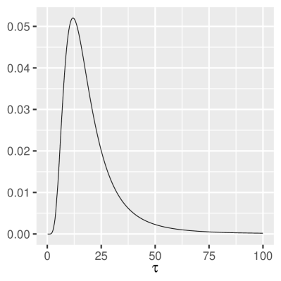
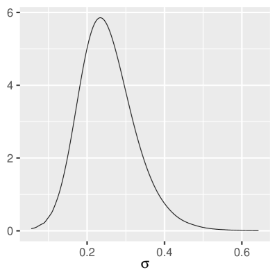
Figure 2: Posterior marginal for the hyperparameter: on the precision scale (left) and on the standard deviation scale (right).

From the transformed posterior marginal the function inla.zmarginal() allows to extract posterior ’z’ummary information:

inla.zmarginal(my.sigma)

## Mean            0.253194
## Stdev           0.0735528
## Quantile  0.025 0.127062
## Quantile  0.25  0.202214
## Quantile  0.5   0.246286
## Quantile  0.75  0.296463
## Quantile  0.975 0.417444

The inla.emarginal() and inla.tmarginal() functions we used above are part of a family of inla.$\star$marginal functions in the R-INLA library that can be used to manipulate univariate posterior marginals in different ways. Table 1 provides a list of such functions with the relative usage.

Function Name	Usage
inla.dmarginal(x, marginal, $\dots$)	Density at a vector of evaluation points $x$
inla.pmarginal(q, marginal, $\dots$)	Distribution function at a vector of quantiles $q$
inla.qmarginal(p, marginal, $\dots$)	Quantile function at a vector of probabilities $p$.
inla.rmarginal(n, marginal)	Generate $n$ random deviates
inla.hpdmarginal(p, marginal, $\dots$)	Compute the highest posterior density interval at level $p$
inla.emarginal(fun, marginal, $\dots$)	Compute the expected value of the marginal assuming the transformation given by fun
inla.mmarginal(marginal)	Computes the mode
inla.smarginal(marginal, $\dots$)	Smoothed density in form of a list of length two. The first entry contains the x-values, the second entry includes the interpolated y-values
inla.tmarginal(fun, marginal, $\dots$)	Transform the marginal using the function fun.
inla.zmarginal(marginal)	Summary statistics for the marginal

Table 1: Functions which use a posterior marginal density to derive some information of interest. The marginal is thereby given in form of a matrix with two columns where the first column represents the location points and the second column the density values at those location points.

Posterior marginals for the fixed effects are stored in result$marginals.fixed. This is a list of length equal to the number of fixed effects in the model plus the intercept (3 in this case). We can obtain the posterior mean of the intercept as follows:

inla.emarginal(function(x) x, result$marginals.fixed$‘(Intercept)‘)

## [1] 2.2

However, note that summary information for all the fixed effects is directly available in the slot result$summary.fixed.

result$summary.fixed

##                 mean      sd 0.025quant 0.5quant 0.97quant     mode
## (Intercept)  2.16813 0.35883     1.4507  2.17009   2.84317  2.17401
## log(x + 10)  0.31294 0.09764     0.1188  0.31300   0.49800  0.31313
## x           -0.00098 0.00043    -0.0018 -0.00098  -0.00016 -0.00098
##                 kld
## (Intercept) 7.6e-07
## log(x + 10) 2.1e-06
## x           2.1e-06

Finally, the marginal densities for the random effects are stored in result$marginals.random$plate (a list with length $18$ elements in this case) while summary statistics for the random effects are stored in result$summary.random$rand. Figure 3 shows the posterior mean of $\bm{u}$ within $2.5\%$ and $97.5\%$ quantiles and is created from information stored in the result$summary.random$u object.

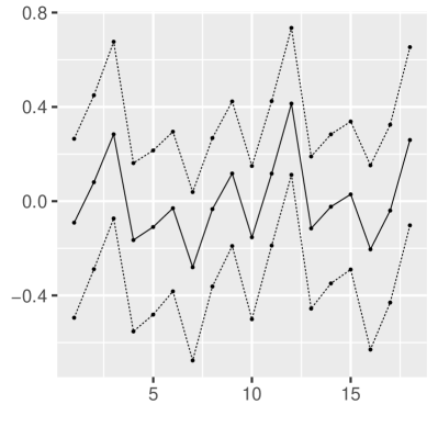
Figure 3: Posterior mean (solid line) together with $2.5\%$ and $97.5\%$ posterior quantiles (broken lines) for the random effect $\bf{u}$

4.3 Getting prediction densities

Posterior predictive distributions are of interest in many applied problems. The inla() function does not return predictive densities. In this Section we show how to post-process the result from inla() in order to obtain the posterior predictive density for a point of interest.

Assume we would like to predict a new datapoint. For ease of illustration we remove datapoint $k=7$ in the Salm dataset and predict it. That is, we are interested in $\pi(y_{7}|\bm{y}_{-7})$ where $\bm{y}_{-7}$ is the vector of all observations except for the $7^{\text{th}}$.

The inla() function allows for missing values in the response variable, and computes the posterior marginal for the corresponding linear predictor. We create a new dataset Salm.predict where observation 7 is set to NA and rerun the inla() function:

## set observation 7 to NA
Salm.predict = Salm
Salm.predict[7, "y"] <- NA
# re-run the model
res.predict = inla(formula=formula, data=Salm,
  family="Poisson",
  control.predictor = list(compute = TRUE),
  control.family = list(control.link=list(model="log"))
  )

Note that, compared to the previous run of inla(), here we have specified some extra parameters. As default, the posterior marginals for the linear predictor are not provided. By specifying control.predictor = list(compute = TRUE) the posterior marginals will be included in the results object. We also need to explicitly specify the link function using the control.family object in order for inla() to compute the linear predictor not only at the linear scale ($\eta$) but also at the observations scale ($\lambda=\exp(\eta)$).

We can inspect the linear predictor $\eta_{7}=\log(\lambda_{7})$ using

# marginal posterior for the linear predictor
eta7 = res.predict$marginals.linear.predictor[[7]]
# some summary statistics
round(res.predict$summary.linear.predictor[7,], 3)

##              mean   sd 0.025quant 0.5quant 0.97quant mode kld
## Predictor.07    3 0.18        2.6        3       3.4  3.1   0

We can then compute the linear predictor at the observation scale $\lambda_{7}=\exp(\eta_{7})$ using the inla.tmarginal() function as before. An alternative, having specified the link function in the control.family() parameter, is to extract $\lambda_{7}$ directly from the result object:

# extract from the res.predict object
lambda7 = res.predict$marginals.fitted.values[[7]]
# compute using inla.tmarginal()
lambda7_bis = inla.tmarginal(function(x){exp(x)},
  res.predict$marginals.linear.predictor[[7]])

Figure 4 shows the posterior marginal $\widetilde{\pi}(\eta_{7}|\bm{y})$ and $\widetilde{\pi}(\lambda_{7}|\bm{y})$.

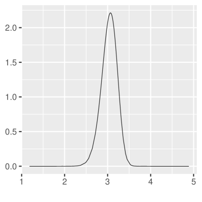
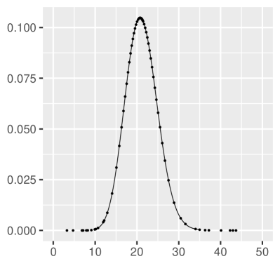
Figure 4: Posterior marginal for the linear predictor (left) and for the linear predictor at the observation scale, i.e. the fitted value scale (right). The last quantity can be directly extracted from the result object (dots) or computed using the inla.tmarginal() function (black line).

The predictive distribution is given by:

$$\widetilde{\pi}(y_{7}|\bm{y}_{-7})=\int\widetilde{\pi}(y_{7}|\lambda_{7})\widetilde{\pi}(\lambda_{7}|\bm{y}_{-7})d\lambda_{7}$$ (9)

We can solve (9) in two ways, by sampling or numerical integration. If we want to sample we need to proceed in two steps: first sample values for $\lambda_{7}$ from its posterior density, then sample possible observations from a Poisson likelihood with mean equal to the sampled values of $\lambda_{7}$:

n.samples = 3000
samples_lambda = inla.rmarginal(n.samples, lambda7)
# sample from the likelihood model
predDist = rpois(n.samples, lambda = samples_lambda)

Figure 5 shows an histogram of the predicted values sampled as above. Note that, in this case, we could sample directly from the posterior marginal of the linear predictor at the observation scale. When the likelihood depends not only in the latent field but also on some hyperparameters (as in the Gaussian case, say) we need to sample both $\eta$ and $\bm{\theta}$ jointly. This can be done using the function inla.posterior.sample() which takes as input the number of samples and the res.predict object and return samples from the joint posterior marginal. In order for this function to work one has to provide the extra parameter control.compute = list(config = TRUE) when calling the inla() function.

A second possibility is to solve (9) numerically as:

 # library supporting trapezoid rule integration.
 library(caTools)

 # specify the support at which we want to compute the density
 ii = 0:100
 predDist2 = rep(0,101)
 # go over the posterior marginal of the fitted value
for(j in 1:(length(lambda7[ ,1])-1)){
  predDist2 <- predDist2 + dpois(ii,
           lambda = ((lambda7[j,1]+ lambda7[j+1,1])/2)) *
             trapz(lambda7[j:(j+1), 1], lambda7[j:(j+1), 2])
 }

A drawback with this method is that one has to locate the area of high density of the predictive distribution in order to perform the integration. Figure 5 shows the prediction distribution as computed above.

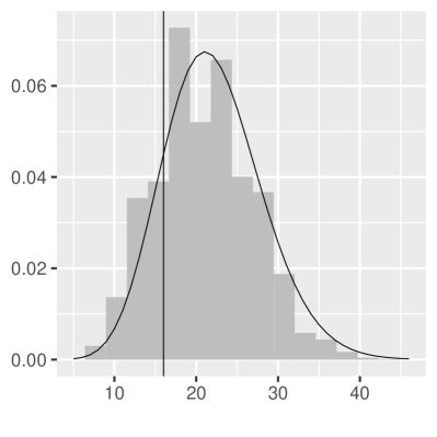
Figure 5: Estimate of the posterior predictive density $\widetilde{\pi}(y_{7}|\bm{y}_{-7})$ via sampling (histogram) and numerical integration (black line). The vertical line indicate the observation $y_{7}$ that we have removed from the dataset.

5 Expanding the scope: INLA within MCMC

Implementing INLA from scratch is a complex task so that, in practice, the applications of INLA are limited to the (large class of) models implemented in the R-INLA library. The library allows the user to manually specify latent Gaussian models, see vignette("rgeneric", package="INLA"), that are not directly available within the library. Also user-defined hyperpriors are possible. However, certain models do not fit into the scope of R-INLA. Consider for example the case in which one observation does not only depend on exactly one element of the linear predictor.

Recently Gómez-Rubio and Rue, ¹² proposed a novel approach that enlarges the class of models that can benefit from the fast computations of INLA. Let $\bm{z}=(\bm{x},\bm{\theta})$ denote all model parameters. Bivand et al., ⁵, noticed that some models can be fit with R-INLA after conditioning on one or several parameters. That is, we split the parameter vector into two, $\bm{z}=(\bm{z}_{c},\bm{z}_{-c})$, and assume that the model

$$\pi(\bm{z}_{-c}|\bm{y},\bm{z}_{c})\propto\pi(\bm{y}|\bm{z}_{-c},\bm{z}_{c})\pi(\bm{z}_{-c}|\bm{z}_{c})$$

can be fit with R-INLA. If the conditioning parameters are few and bounded, one way to solve the full model is to define a grid $\bm{z}^{k}_{c}$, $k=1,\dots,K$ on the bounded domain of the conditioning parameters and run inla() on all $K$ conditional models. At each run we get approximations to the marginal likelihood $\tilde{\pi}(\bm{y}|\bm{z}_{c}^{k})$ and to the (conditional) posterior marginals $\tilde{\pi}(z_{-c,j}|\bm{y},\bm{z}_{c}^{k})$ for each element $j$ of vector $\bm{z}_{-c}$. The posterior for the conditioning parameters $\bm{z}_{c}$ can be obtained combining the marginal likelihood with the prior:

$$\tilde{\pi}(\bm{z}_{c}^{k}|\bm{y})\propto\tilde{\pi}(\bm{y}|\bm{z}_{c}^{k})\pi(\bm{z}_{c}^{k})$$

This can be easily normalized since we assume a bounded domain. For the remainder of the parameters $\bm{z}_{-c}$, their posterior marginal distribution can be obtained by Bayesian model averaging the family of models fitted with R-INLA:

$$\pi(z_{-c,j}|\bm{y})=\int\pi(z_{-c,j}|\bm{y},\bm{z}_{c})\pi(\bm{z}_{c}|\bm{y})d\bm{z}_{c}\approx\sum_{k}\tilde{\pi}(z_{-c,j}|\bm{y},\bm{z}_{c}^{k})\tilde{\pi}(\bm{z}_{c}^{k}|\bm{y}).$$ (10)

This solution, becomes infeasible if $\bm{z}_{c}$ is larger and unbounded.

Gómez-Rubio and Rue, ¹² propose instead to embed INLA in a larger Metropolis–Hastings (MH) algorithm ²³, ¹⁶. In this way, the posterior marginals of an ensemble of parameters (namely those we condition on) can be obtained via MCMC sampling, whereas the posterior marginals of all the other parameters are obtained by averaging over several conditional marginal distributions.

To estimate the posterior distribution of all parameters in the model, the MH algorithm can be used to draw values for $\bm{z}_{c}$. At step $i$, new values $\bm{z}_{c}^{(i)}$ are proposed and accepted with probability

$$\alpha=\min\left\{1,\frac{\pi(\bm{y}|\bm{z}_{c}^{(i)})\pi(\bm{z}_{c}^{(i)})}{\pi(\bm{y}|\bm{z}_{c}^{(i-1)})\pi(\bm{z}_{c}^{(i-1)})}\frac{q(\bm{z}_{c}^{(i-1)}|\bm{z}_{c}^{(i)})}{q(\bm{z}_{c}^{(i)}|\bm{z}_{c}^{(i-1)})}\right\}$$ (11)

If the proposal is not accepted, then $\bm{z}_{c}^{(i)}$ is set to $\bm{z}_{c}^{(i-1)}$.

For each proposed value of the conditioning parameters $\bm{z}_{c}^{(i)}$ we run inla() on the conditional model and obtain the approximated posterior (conditional) marginals for all parameters in $\bm{z}_{-c}$, $\tilde{\pi}(z_{-c,j}|\bm{y},\bm{z}_{c}^{(i)})$. Note that, in this context we are free to choose any prior for $\bm{z}_{c}$.

After a suitable number of iterations, the MH algorithm will produce $N$ samples from $\pi(\bm{z}_{c}|\bm{y})$ which can be used to derive posterior marginals or any other summary statistics of interest. The posterior marginals for the parameters in $\bm{z}_{-c}$ can be approximated as

$$\tilde{\pi}(z_{-c,j}|\bm{y})=\frac{1}{N}\sum_{i}\tilde{\pi}(z_{-c,j}|\bm{y},\bm{z}_{c}^{(i)}).$$

Note that using INLA within MCMC allows to perform multivariate posterior inference on the parameter subset $\bm{z}_{c}$.

Gómez-Rubio and Rue, ¹² illustrate the use of INLA within MCMC with different examples including some spatial econometrics models, Bayesian lasso and imputation of missing covariates. They show that the new algorithm provides accurate approximations to the posterior distribution. Wilson and Wakefield, ³⁶ use INLA within MCMC to correct for jittering in the locations of complex survey studies. INLA within MCMC can be used to fit models where non-Gaussian or multivariate priors are used on some elements of the latent field and hyperparameters. It can also be used in cases where the user wants to model both parameters in the likelihood (for example the mean and the standard deviation in the Gaussian likelihood) with respect to some covariates. This method largely increases the class of models that can benefit of the powerful computational machinery of INLA. Moreover, it allows to perform multivariate inference on a small set of model parameters.

In the INLA within MCMC context, the inla() function can be seen as a device to reduce the dimensionality of the model so that one has to focus only on a smaller subset of parameters $\bm{z}_{c}$. Implementation is also simpler compared to the one of a full MCMC algorithm. INLA within MCMC is a computationally intensive and sequential algorithm and might take time to converge. Moreover, the present implementation of the inla() program is not optimal in this context as it creates a large amount of temporary files every time the model is run. Gómez-Rubio and Palmí-Perales, ¹⁵ explore simpler alternatives to the full INLA within MCMC approach useful when fitting complex spatial models. These simple alternatives are based on exploring the posterior of the conditioning parameters $\bm{z}_{c}$ by using a central composite design or simply fixing their value at posterior mode.

6 Discussion

Since its introduction, INLA has established itself as a powerful tool to perform Bayesian analysis on LGMs. The associated R-INLA package has made INLA a practical and relatively straight forward tool that has reached practitioners in a wide range of applied field, see Rue et al., ²⁸ for a review of applications. The R-INLA package aims at being as general as possible within the class of LGM. It provides a large selection of likelihoods, latent models and priors to choose from, and the possibility to add some user defined latent models and priors. It is possible to simultaneously model data from different likelihoods, replicate and copy parts of the latent fields and several other features, see Rue et al., ²⁸, Martins et al., ²¹ and www.r-inla.org. Recent developments aim to extend the scope of INLA by combining it with MCMC techniques.

For some of the end-users, interested only in a sub-class of the possible LGMs, the generality of R-INLA comes at the cost of increased complexity and lack of more specific tools. In the years, a series of add-on packages have been created to improve accessibility for a specific target audience and to provide specialized tools that are mainly relevant for the specific class of models under considerations. Table 6 collects a list of such add-on packages the authors are aware of. For each package a short description of its purpose is reported together with a reference and a url address for download.

Package name	Purpose	Reference	Download
AnimalINLA	Analysis of “animal models”/additive genetic models/pedigree based models	Holand et al., 18	https://folk.ntnu.no/annamaho/AnimalINLA/AnimalINLA_1.4
ShrinkBayes	Shrinkage priors with applications to RNA sequencing	Van De Wiel et al., 34	https://github.com/markvdwiel/ShrinkBayes
meta4diag	Bayesian inference for bivariate meta-analysis of diagnostic test studies	Guo and Riebler, 14	https://cran.r-project.org/web/packages/meta4diag
BAPC	Bayesian age-period-cohort models with focus on projections	Riebler and Held, 25	https://rdrr.io/rforge/BAPC/man/BAPC.html
diseasemapping	Formatting of population and case data, calculation of Standardized Incidence Ratios, and fitting the BYM model using INLA.	Brown, 8	https://rdrr.io/rforge/diseasemapping/
geostatp	Geostatistical modelling facilities using Raster and SpatialPoints objects. Non-Gaussian models are fit using INLA.	Brown, 8	https://cran.r-project.org/web/packages/geostatsp
excursions	Excursion sets, contour credible regions, and simultaneous confidence bands	Bolin and Lindgren, 6	https://cran.r-project.org/web/packages/excursions
INLABRU	Model spatial distribution and change from ecological survey data	www.inlabru.org	https://cran.r-project.org/web/packages/inlabru
INLABMA	Spatial Econometrics models using Bayesian model averaging and MCMC inla	Bivand et al., 4	https://cran.r-project.org/web/packages/INLABMA
nmaINLA	Performs network meta-analysis using INLA. Includes methods to assess the heterogeneity and inconsistency in the network.	Guenhan et al., 13	https://cran.r-project.org/web/packages/nmaINLA
INLAutils	Utility Functions for INLA: Additional Plots and Support for ggplot2.		https://rdrr.io/github/timcdlucas/INLAutils
abn	Modelling Multivariate Data with Additive Bayesian Networks		https://CRAN.R-project.org/package=abn
BCEA	Bayesian Cost Effectiveness Analysis	Baio and Dawid, 1	https://CRAN.R-project.org/package=BCEA
DClusterm	Model-based methods for the detection of disease clusters using GLMs, GLMMs and zero-inflated models.	Gómez-Rubio et al., 11	https://CRAN.R-project.org/package=DClusterm
PrevMap	Geostatistical Modelling of Spatially Referenced Prevalence Data	Giorgi and Diggle, 10	https://CRAN.R-project.org/package=PrevMap
SUMMER	Provides methods for estimating, projecting, and plotting spatio-temporal under-five mortality rates.	Mercer et al., 22	https://CRAN.R-project.org/package=SUMMER
surveillance	Temporal and Spatio-Temporal Modeling and Monitoring of Epidemic Phenomena	Salmon et al., 29, Meyer et al., 24	https://CRAN.R-project.org/package=surveillance
survHE	Survival Analysis in Health Economic Evaluation		https://CRAN.R-project.org/package=survHE
List of add-on packages build around R-INLA for specialized sub-classes of LGMs.

References

- Baio and Dawid, 2011 Baio, G. and Dawid, A. P. (2011). Probabilistic sensitivity analysis in health economics. Statistical Methods in Medical Research.
- Bakka et al., 2018 Bakka, H., Rue, H., Fuglstad, G.-A., Riebler, A., Bolin, D., Illian, J., Krainski, E., Simpson, D., and Lindgren, F. (2018). Spatial modeling with R-INLA: A review. Wiley Interdisciplinary Reviews: Computational Statistics, 10(6):e1443.
- Besag et al., 1991 Besag, J., York, J., and Mollié, A. (1991). Bayesian image restoration, with two applications in spatial statistics. Annals of the Institute of Statistical Mathematics, 43(1):1–20.
- Bivand et al., 2015 Bivand, R. S., Gómez-Rubio, V., and Rue, H. (2015). Spatial data analysis with R-INLA with some extensions. Journal of Statistical Software, 63(20):1–31.
- Bivand et al., 2014 Bivand, R. S., Gómez-Rubio, V., and Rue, H. (2014). Approximate Bayesian inference for spatial econometrics models. Spatial Statistics, 9:146 – 165.
- Bolin and Lindgren, 2015 Bolin, D. and Lindgren, F. (2015). Excursion and contour uncertainty regions for latent Gaussian models. Journal of the Royal Statistical Society: Series B (Statistical Methodology), 77(1):85–106.
- Breslow, 1984 Breslow, N. E. (1984). Extra-poisson variation in log-linear models. Journal of the Royal Statistical Society. Series C (Applied Statistics), 33(1):38–44.
- Brown, 2015 Brown, P. (2015). Model-based geostatistics the easy way. Journal of Statistical Software, Articles, 63(12):1–24.
- Ferkingstad and Rue, 2015 Ferkingstad, E. and Rue, H. (2015). Improving the INLA approach for approximate Bayesian inference for latent Gaussian models. Electron. J. Statist., 9(2):2706–2731.
- Giorgi and Diggle, 2017 Giorgi, E. and Diggle, P. (2017). Prevmap: An r package for prevalence mapping. Journal of Statistical Software, Articles, 78(8):1–29.
- Gómez-Rubio et al., 2018 Gómez-Rubio, V., Molitor, J., and Moraga, P. (2018). Fast bayesian classification for disease mapping and the detection of disease clusters. In Cameletti, M. and Finazzi, F., editors, Quantitative Methods in Environmental and Climate Research, pages 1–27, Cham. Springer International Publishing.
- Gómez-Rubio and Rue, 2018 Gómez-Rubio, V. and Rue, H. (2018). Markov chain Monte Carlo with the integrated nested Laplace approximation. Statistics and Computing, 28(5):1033–1051.
- Guenhan et al., 2018 Guenhan, B. K., Friede, T., and Held, L. (2018). A design-by-treatment interaction model for network meta-analysis and meta-regression with integrated nested Laplace approximations. Research Synthesis Methods, pages 179–194.
- Guo and Riebler, 2018 Guo, J. and Riebler, A. (2018). meta4diag: Bayesian bivariate meta-analysis of diagnostic test studies for routine practice. Journal of Statistical Software, Articles, 83(1):1–31.
- Gómez-Rubio and Palmí-Perales, 2019 Gómez-Rubio, V. and Palmí-Perales, F. (2019). Multivariate posterior inference for spatial models with the integrated nested Laplace approximation. Journal of the Royal Statistical Society: Series C (Applied Statistics), 68(1):199–215.
- Hastings, 1970 Hastings, W. K. (1970). Monte Carlo sampling methods using Markov chains and their applications. Biometrika, 57(1):97–109.
- Held et al., 2010 Held, L., Schrödle, B., and Rue, H. (2010). Posterior and cross-validatory predictive checks: A comparison of MCMC and INLA. In Statistical Modelling and Regression Structures. Physica-Verlag HD.
- Holand et al., 2013 Holand, A., Steinsland, I., Martino, S., and Jensen, H. (2013). Animal models and integrated nested Laplace approximations. G3 (Bethesda), 8(3):1241–1251.
- Hubin and Storvik, 2016 Hubin, A. and Storvik, G. (2016). Estimating the marginal likelihood with integrated nested Laplace approximation (INLA). arXiv e-prints, page arXiv:1611.01450.
- Lindgren et al., 2011 Lindgren, F., Rue, H., and Lindström, J. (2011). An explicit link between Gaussian fields and Gaussian Markov random fields: the stochastic partial differential equation approach. Journal of the Royal Statistical Society, Series B (Statistical Methodology), 73(4):423–498.
- Martins et al., 2013 Martins, T. G., Simpson, D., Lindgren, F., and Rue, H. (2013). Bayesian computing with INLA: new features. Computational Statistics & Data Analysis, 67:68–83.
- Mercer et al., 2015 Mercer, L. D., Wakefield, J., Pantazis, A., Lutambi, A. M., Masanja, H., and Clark, S. (2015). Space–time smoothing of complex survey data: Small area estimation for child mortality. Ann. Appl. Stat., 9(4):1889–1905.
- Metropolis et al., 1953 Metropolis, N., Rosenbluth, A. W., Rosenbluth, M. N., Teller, A. H., and Teller, E. (1953). Equation of state calculations by fast computing machines. The Journal of Chemical Physics, 21(6):1087–1092.
- Meyer et al., 2017 Meyer, S., Held, L., and Höhle, M. (2017). Spatio-temporal analysis of epidemic phenomena using the R package surveillance. Journal of Statistical Software, 77(11):1–55.
- Riebler and Held, 2017 Riebler, A. and Held, L. (2017). Projecting the future burden of cancer: Bayesian age–period–cohort analysis with integrated nested Laplace approximations. Biometrical Journal, 59(3):531–549.
- Rue and Held, 2005 Rue, H. and Held, L. (2005). Gaussian Markov Random Fields: Theory And Applications (Monographs on Statistics and Applied Probability). Chapman & Hall/CRC.
- Rue et al., 2009 Rue, H., Martino, S., and Chopin, N. (2009). Approximate Bayesian inference for latent Gaussian models by using integrated nested Laplace approximations. Journal of the Royal Statistical Society: Series B (Statistical Methodology), 71(2):319–392.
- Rue et al., 2017 Rue, H., Riebler, A., Sørbye, S. H., Illian, J. B., Simpson, D. P., and Lindgren, F. K. (2017). Bayesian computing with INLA: A review. Annual Review of Statistics and Its Application, 4(1):395–421.
- Salmon et al., 2016 Salmon, M., Schumacher, D., and Höhle, M. (2016). Monitoring count time series in R: Aberration detection in public health surveillance. Journal of Statistical Software, 70(10):1–35.
- Sauter and Held, 2016 Sauter, R. and Held, L. (2016). Quasi-complete separation in random effects of binary response mixed models. Journal of Statistical Computation and Simulation, 86(14):2781–2796.
- Simpson et al., 2017 Simpson, D., Rue, H., Riebler, A., Martins, T. G., and Sørbye, S. H. (2017). Penalising model component complexity: A principled, practical approach to constructing priors. Statist. Sci., 32(1):1–28.
- Spiegelhalter et al., 2002 Spiegelhalter, D. J., Best, N. G., Carlin, B. P., and Van Der Linde, A. (2002). Bayesian measures of model complexity and fit. Journal of the Royal Statistical Society: Series B (Statistical Methodology), 64(4):583–639.
- Tierney and Kadane, 1986 Tierney, L. and Kadane, J. B. (1986). Accurate approximations for posterior moments and marginal densities. Journal of the American Statistical Association, 81(393):82–86.
- Van De Wiel et al., 2012 Van De Wiel, M. A., Leday, G. G., Pardo, L., Rue, H., Van Der Vaart, A. W., and Van Wieringen, W. N. (2012). Bayesian analysis of RNA sequencing data by estimating multiple shrinkage priors. Biostatistics, 14(1):113–128.
- Watanabe, 2010 Watanabe, S. (2010). Asymptotic equivalence of Bayes cross validation and widely applicable information criterion in singular learning theory. J. Mach. Learn. Res., 11:3571–3594.
- Wilson and Wakefield, 2019 Wilson, K. and Wakefield, J. (2019). Spatial modeling with incomplete data location information. Technical report, University of Washington. in preparation.
- Wood, 2017 Wood, S. (2017). Generalized Additive Models: An Introduction with R. Chapman and Hall/CRC, 2 edition.