Yanxia Qian,  Shuonan Wu,  Fei Wang

Abstract. The Brinkman equations can be regarded as a combination of the Stokes and Darcy equations which model transitions between the fast flow in channels (governed by Stokes equations) and the slow flow in porous media (governed by Darcy’s law). The numerical challenge for this model is the designing of a numerical scheme which is stable for both the Stokes-dominated (high permeability) and the Darcy-dominated (low permeability) equations. In this paper, we solve the Brinkman model in $n$ dimensions ($n=2,3$) by using the mixed discontinuous Galerkin (MDG) method, which meets this challenge. This MDG method is based on the pseudostress-velocity formulation and uses a discontinuous piecewise polynomial pair $\underline{\bm{\mathcal{P}}}_{k+1}^{\mathbb{S}}$-$\bm{\mathcal{P}}_{k}$ $(k\geq 0)$, where the stress field is symmetric. The main unknowns are the pseudostress and the velocity, whereas the pressure is easily recovered through a simple postprocessing. A key step in the analysis is to establish the parameter-robust inf-sup stability through specific parameter-dependent norms at both continuous and discrete levels. Therefore, the stability results presented here are uniform with respect to the permeability. Thanks to the parameter-robust stability analysis, we obtain optimal error estimates for the stress in broken $\underline{\bm{H}}(\bm{{\rm div}})$-norm and velocity in $\bm{L}^{2}$-norm. Furthermore, the optimal $\underline{\bm{L}}^{2}$ error estimate for pseudostress is derived under certain conditions. Finally, numerical experiments are provided to support the theoretical results and to show the robustness, accuracy, and flexibility of the MDG method.

Keywords. Brinkman model, mixed discontinuous Galerkin method, pseudostress, parameter-robust stability

1 Introduction

The Brinkman equations (cf. [18]),

$$\nu\bm{\underline{\bm{\kappa}}}^{-1}\bm{u}-2\nu\mathbf{div}(\underline{\bm{\varepsilon}}(\bm{u}))+\nabla p =\bm{f} \text{in }\Omega,$$ (1.1a)

$${\rm div}\bm{u} =0 \text{in }\Omega,$$ (1.1b)

which model the flow of a fluid through a complex porous medium occupying domain $\Omega$ with a high-contrast permeability tensor $\underline{\bm{\kappa}}$, can be seen as a mixture of Darcy and Stokes equations. Here, $\nu>0$ is the fluid viscosity, $\bm{u}$ denotes the velocity field, $\underline{\bm{\varepsilon}}(\bm{u})=(\underline{\bm{\nabla}}\bm{u}+(\underline{\bm{\nabla}}\bm{u})^{t})/2$ is the strain rate, $p$ is the pressure field, and $\bm{f}$ is the volume force. This model arises from applications in many fields, such as groundwater hydrology, biomedical engineering, petroleum industry, and environmental science (cf. [51, 41, 47]). From (1.1), we can see that the Brinkman problem becomes Stokes-dominated when the permeability tensor $\underline{\bm{\kappa}}$ is getting large, and it becomes Darcy-dominated when $\underline{\bm{\kappa}}$ is quite small.

It is well known that the usual Darcy stable element pairs may diverge for Stokes flow and vice versa. Therefore, the numerical challenge for solving the Brinkman model is to construct a stable discretization method for both the Stokes and the Darcy equations. As shown in [42], the Darcy stable finite element pairs, for example, the Raviart-Thomas element (cf. [44]) leads to non-convergent results as the Brinkman model becomes Stokes-dominated; on the other hand, the usual Stokes stable finite element pairs, such as Mini-element (cf. [3]), $\bm{\mathcal{P}_{2}}$-$\mathcal{P}_{0}$ element, nonconforming Crouzeix-Raviart (CR) finite element (cf. [24]), will diverge when the Brinkman equations turn into Darcy-dominated. Therefore, many researchers pay attention to developing stable and accurate numerical methods for solving Brinkman equations. One way to circumvent this difficulty is to modify the existing Stokes or Darcy elements to make them work well for the Brinkman model. In [19], inspired by discontinuous Galerkin (DG) method, a stabilized CR finite element method is constructed by adding a penalty term. In addition, a generalization of classical Mini-element is studied in [37]; stabilized equal-order finite elements are proposed and analyzed in [11]; (hybridized) interior penalty DG scheme with $\bm{H}(\rm div)$-conforming finite elements is investigated in [39]. Another approach is to develop new numerical schemes for solving Brinkman equations, for examples, pseudostress-based mixed finite element methods (cf. [5, 26]), weak Galerkin methods (cf. [43, 53]), virtual element method (cf. [20]), hybrid high-order method (cf. [10]) and hybridizable discontinuous Galerkin method (cf. [29]).

To study hydrodynamics, different formulations, like velocity-pressure, stress-velocity-pressure, pseudostress-velocity formulations, have been introduced and analyzed. The velocity-pressure formulation has been extensively studied in the computation of incompressible Newtonian flows (cf. [15, 9]). However, the study of numerical methods for the stress-based and pseudostress-based formulations (cf. [25, 7, 21, 27]) has become a very active research area because of the arising interest in non-Newtonian flows. The main advantage of the stress-based and pseudostress-based formulation is that it provides a unified framework for both the Newtonian and the non-Newtonian flows. In addition, physical quantity like the stress can be computed directly instead of by taking derivatives of the velocity, which avoids degrading of accuracy in the process of numerical differentiation. Precise computation of the stress is of paramount importance for the hydraulic fracturing problem as the crack propagation is determined by the stress field. While a formulation comprising the stress as a fundamental unknown is unavoidable for non-Newtonian flows in which the constitutive law is nonlinear, the drawback of the stress-velocity-pressure formulation is the increase in the number of unknowns. To avoid this disadvantage, we focus on the pseudostress-velocity formulation. Last but not least, we need to mention that the pressure field can be easily obtained by a simple postprocessing without affecting the accuracy of the approximation.

Due to the flexibility in constructing the local shape function spaces and the ability to capture non-smooth or oscillatory solutions effectively, DG methods have been applied to solve many problems in scientific computing and engineering, such as conservation laws (cf. [8, 22]), Darcy flow (cf. [16, 1]), Navier-Stokes (or Stokes) equations (cf. [6, 38]), variational inequalities (cf. [49, 12, 48]) and much more. Besides, DG methods also enjoy the following advantages: (i) locally (and globally) conservative; (ii) easy to implement $hp$ adaptivity; (iii) suitable for parallel computing. We refer to [23, 17, 2, 32] for more discussion about DG methods.

In this paper, we construct a mixed discontinuous Galerkin (MDG) method with $\underline{\bm{\mathcal{P}}}_{k+1}^{\mathbb{S}}$-$\bm{\mathcal{P}}_{k}$ element pair for solving the Brinkman equations based on the pseudostress-velocity formulation. The main results of this article include that: (i) The MDG scheme with symmetric stress field is uniformly stable and efficient for both Darcy-dominated and Stokes-dominated flows; (ii) Under specific parameter-dependent norms, the parameter-robust stability results of both continuous and discrete schemes are obtained; (iii) For $k\geq 0$, we get the optimal convergence order for the stress in broken $\underline{\bm{H}}(\bm{{\rm div}})$-norm and velocity in $\bm{L}^{2}$-norm; (iv) When $k\geq n$ and the Stokes pair $\bm{\mathcal{P}}_{k+2}$-$\mathcal{P}_{k+1}$ is stable, we obtain the optimal $\underline{\bm{L}}^{2}$ error estimate for the pseudostress.

The rest of the paper is organized as follows. In Section 2, we introduce the pseudostress-velocity formulation for the Brinkman model and present some preliminary results. In Section 3, the MDG scheme is introduced and the well-posedness is obtained. We show the stability of the discrete scheme and prove optimal error estimates for both velocity and pressure in Section 4. In Section 5, numerical examples are provided to confirm the theoretical findings and to illustrate the performance of the mixed DG scheme. Finally, we give a short summary in Section 6.

2 Brinkman model in pseudostress-velocity formulation

In this section, we introduce the Brinkman model in the pseudostress-velocity formulation and provide the parameter-robust stability analysis of the continuous problem. First, we give the notation.

2.1 Notation

Given $n$ ($n=2$ or $3$), we denote the space of real matrices of order $n\times n$ by $\mathbb{M}$, and define $\mathbb{S}\subset\mathbb{M}$ as the space of real symmetric matrices. For matrices $\underline{\bm{\tau}}=(\tau_{ij})\in\mathbb{M}$ and $\underline{\bm{\zeta}}=(\zeta_{ij})\in\mathbb{M}$, we write as usual

$$\underline{\bm{\tau}}^{t}=(\tau_{ji}),\quad{\rm tr}(\underline{\bm{\tau}})=\sum_{i=1}^{n}\tau_{ii},\quad\underline{\bm{\tau}}^{d}=\underline{\bm{\tau}}-\frac{1}{n}{\rm tr}(\underline{\bm{\tau}})\underline{\bm{I}},\quad\underline{\bm{\tau}}:\underline{\bm{\zeta}}=\sum_{i,j=1}^{n}\tau_{ij}\zeta_{ij},$$ (2.1)

where $\underline{\bm{I}}$ is the identity matrix.

For a subdomain $D\subset\mathbb{R}^{n}$ and integer $m\geq 0$, we denote the scalar-valued Sobolev spaces by $H^{m}(D)=W^{m,2}(D)$ with the norm $\|\cdot\|_{m,D}$ and seminorm $|\cdot|_{m,D}$. When $m=0$, $H^{0}(D)$ coincides with the Lebesgue spaces $L^{2}(D)$, which is equipped with the usual $L^{2}$-inner product $(\cdot,\cdot)_{D}$ and $L^{2}$-norm $||\cdot||_{0,D}$. The $L^{2}$-inner product (or duality pairing) on $\partial D$ is denoted by $\langle\cdot,\cdot\rangle_{\partial D}$. We denote the vector-valued spaces, tensor-valued function spaces and symmetric-tensor-valued spaces whose entries are in $H^{m}(D)$ by $\bm{H}^{m}(D)$, $\underline{\bm{H}}^{m}(D)$ and $\underline{\bm{H}}^{m}(D;\mathbb{S})$, respectively. In particular, $\bm{H}^{0}(D)=\bm{L}^{2}(D)$, $\underline{\bm{H}}^{0}(D)=\underline{\bm{L}}^{2}(D)$ and $\underline{\bm{H}}^{0}(D;\mathbb{S})=\underline{\bm{L}}^{2}(D;\mathbb{S})$. Then, we introduce the following space

$$\underline{\bm{H}}(\bm{{\rm div}},D;\mathbb{M})=\{\underline{\bm{\tau}}\in\underline{\bm{L}}^{2}(D;\mathbb{M}):\mathbf{div}\underline{\bm{\tau}}\in\bm{L}^{2}(D)\},$$

equipped with the norm $\|\underline{\bm{\tau}}\|_{\bm{{\rm div}},D}=(\|\underline{\bm{\tau}}\|^{2}_{0,D}+\|\mathbf{div}\underline{\bm{\tau}}\|^{2}_{0,D})^{1/2}$ for all $\underline{\bm{\tau}}\in\,\underline{\bm{H}}(\bm{{\rm div}};\mathbb{M})$. Here, differential operators are applied row by row, i.e., the $i$-th row of $\bm{{\rm div}}\underline{\bm{\sigma}}$ is the divergence of the $i$-th row vector of the matrix $\underline{\bm{\sigma}}$. Similarly, the $i$-th row of the matrix $\underline{\bm{\nabla}}\bm{u}$ in the definition of $\underline{\bm{\varepsilon}}(\bm{u})$ is the gradient (written as a row) of the $i$-th component of the vector $\bm{u}$. We also define $\underline{\bm{H}}(\bm{{\rm div}},D;\mathbb{S})=\{\underline{\bm{\tau}}\in\underline{\bm{L}}^{2}(D;\mathbb{S}):\mathbf{div}\underline{\bm{\tau}}\in\bm{L}^{2}(D)\}$.

In the present context, Green’s formula takes the form

$$(\underline{\bm{\varepsilon}}(\bm{v}),\underline{\bm{\tau}})_{D}=-(\mathbf{div}\underline{\bm{\tau}},\bm{v})_{D}+\langle\underline{\bm{\tau}}\bm{n}_{D},\bm{v}\rangle_{\partial D},$$ (2.2)

where $\bm{n}_{D}$ is the exterior unit normal to $\partial D$. If $D$ is chosen as $\Omega$, we abbreviate it by using $(\cdot,\cdot)$ and $\langle\cdot,\cdot\rangle$, and similar rule follows for the spaces and norms mentioned above.

2.2 Brinkman model

Let $\Omega\subset\mathbb{R}^{n}$ be a bounded and simply connected polygonal domain with Lipschitz boundary $\Gamma$. In this paper, we consider the permeability of the form $\underline{\bm{\kappa}}=\kappa\underline{\bm{I}}$, with the purpose of facilitating parameter-robust stability analysis. We could also take $\nu=1$ by a non-dimensionalization procedure (see Remark 2.1 below). With these simplifications, we find that for the unique solution ($\bm{u}$, $p$) of the Brinkman model (1.1), ($\underline{\bm{\sigma}}$, $\bm{u}$, $p$) solves the equations

$$\underline{\bm{\sigma}}=2\underline{\bm{\varepsilon}}(\bm{u})-p\underline{\bm{I}}\qquad \text{in }\Omega,$$ (2.3a)

$$\kappa^{-1}\bm{u}-\mathbf{div}\underline{\bm{\sigma}}=\bm{f} \text{in }\Omega,$$ (2.3b)

$${\rm div}\bm{u}=0 \text{in }\Omega,$$ (2.3c)

$$\bm{u}=\bm{g} \text{on }\Gamma,$$ (2.3d)

$$\int_{\Omega}pd\bm{x}=0.$$ (2.3e)

Additionally, due to the incompressibility condition, we assume that $\bm{g}$ satisfies the compatibility condition $\int_{\Gamma}\bm{g}\cdot\bm{n}ds=0$, where $\bm{n}$ stands for the unit outward normal on $\Gamma$.

Remark 2.1.

If $\nu\neq 1$, by taking $\underline{\widetilde{\bm{\sigma}}}=\underline{\bm{\sigma}}/\nu$, $\widetilde{\bm{f}}=\bm{u}/{\nu}$ and $\widetilde{p}=p/{\nu}$, we could eliminate the parameter $\nu$, i.e.

$$\underline{\widetilde{\bm{\sigma}}}=2\underline{\bm{\varepsilon}}(\bm{u})-\widetilde{p}\underline{\bm{I}}\qquad \text{in }\Omega,$$

$$\kappa^{-1}\bm{u}-\mathbf{div}\underline{\widetilde{\bm{\sigma}}}=\widetilde{\bm{f}} \text{in }\Omega,$$

$${\rm div}\bm{u}=0 \text{in }\Omega,$$

$$\bm{u}=\bm{g} \text{on }\Gamma,$$

$$\int_{\Omega}\widetilde{p}d\bm{x}=0.$$

As a result, we can get the same conclusions with the problem (2.3).

As described in Section 1, in order to keep the strengths and improve the weaknesses of the stress-velocity-pressure formulation, by the incompressible condition, the problem (2.3) can be rewritten equivalently as the pseudostress-velocity formulation (cf. [29]):

$$\underline{\bm{\sigma}}^{d}=2\underline{\bm{\varepsilon}}(\bm{u}) \text{in }\Omega,$$ (2.4a)

$$\kappa^{-1}\bm{u}-\mathbf{div}\underline{\bm{\sigma}}=\bm{f} \text{in }\Omega,$$ (2.4b)

$$\bm{u}=\bm{g} \text{on }\Gamma,$$ (2.4c)

$$\int_{\Omega}{\rm tr}(\underline{\bm{\sigma}})d\bm{x}=0,$$ (2.4d)

where the pressure $p$ can be obtained by the postprocessing formula

$$p=-\frac{1}{n}{\rm tr}(\underline{\bm{\sigma}})\qquad\qquad\qquad\text{in }\Omega.$$ (2.5)

There are two reasons for eliminating the pressure. An obvious one is to reduce one variable and, hence, many degrees of freedom in the discrete system. A more important reason is that we can use economic and accurate stable elements and develop fast solvers for the resulting discrete system so that computational cost will be greatly reduced.

Set $\underline{\bm{\Sigma}}=\{\underline{\bm{\tau}}\in\underline{\bm{H}}(\bm{{\rm div}};\mathbb{S}):\int_{\Omega}{\rm tr}(\underline{\bm{\tau}})d\bm{x}=0\}$ and $\bm{V}=\bm{L}^{2}(\Omega)$. Then, the variational formulation of (2.4) reads as follows: given $\bm{f}\in\bm{L}^{2}(\Omega)$ and $\bm{g}\in\bm{H}^{1/2}(\Gamma)$, find $(\underline{\bm{\sigma}},\bm{u})\in\underline{\bm{\Sigma}}\times\bm{V}$ such that

$$a(\underline{\bm{\sigma}},\underline{\bm{\tau}})+b(\underline{\bm{\tau}},\bm{u}) =\langle\underline{\bm{\tau}}\bm{n},\bm{g}\rangle_{\Gamma} \forall\underline{\bm{\tau}}\in\underline{\bm{\Sigma}},$$ (2.6a)

$$b(\underline{\bm{\sigma}},\bm{v})-s(\bm{u},\bm{v}) =-(\bm{f},\bm{v}) \forall\bm{v}\in\bm{V}.$$ (2.6b)

Here, the bilinear forms are defined by

$$a(\underline{\bm{\sigma}},\underline{\bm{\tau}})=\frac{1}{2}(\underline{\bm{\sigma}}^{d},\underline{\bm{\tau}}^{d}),\quad b(\underline{\bm{\tau}},\bm{v})=(\mathbf{div}\underline{\bm{\tau}},\bm{v})\quad{\rm and}\quad s(\bm{u},\bm{v})=(\kappa^{-1}\bm{u},\bm{v}).$$

Notice that, by Green’s formula, the equation (2.6a) contains both the equation $2\underline{\bm{\varepsilon}}(\bm{u})=\underline{\bm{\sigma}}^{d}$ in $\Omega$ and the boundary condition $\bm{u}=\bm{g}$, with in particular the incompressibility condition ${\rm div}\,\bm{u}=\frac{1}{2}{\rm tr}(\underline{\bm{\sigma}}^{d})=0$.

Furthermore, by the definition of $\underline{\bm{\tau}}^{d}$, it is easy to check that

$$\|\underline{\bm{\tau}}\|_{0}^{2}=\|\underline{\bm{\tau}}^{d}\|_{0}^{2}+\frac{1}{n}\|{\rm tr}(\underline{\bm{\tau}})\|_{0}^{2},$$ (2.7)

$$\|{\rm tr}(\underline{\bm{\tau}})\|_{0}\leq\sqrt{n}\|\bm{\tau}\|_{0}.$$ (2.8)

Throughout the paper, we use the abbreviation $x\lesssim y$ ($x\gtrsim y$) for the inequality $x\leq Cy$ ($x\geq Cy$), where the letter $C$ denotes a positive constant independent of the parameters $\kappa$, $\nu$, and the mesh size $h$, and may stand for different values at its different occurrences.

2.3 Well-posedness of the continuous problem

Due to the large variation of the permeability tensor, in order to show that our analysis is independent of the parameters $\kappa$, $\underline{\bm{\Sigma}}$ and $\bm{V}$ are endowed with the norm

$$\|\underline{\bm{\tau}}\|_{\underline{\bm{\Sigma}}}^{2} =(\underline{\bm{\tau}}^{d},\underline{\bm{\tau}}^{d})+\widetilde{\kappa}(\mathbf{div}\underline{\bm{\tau}},\mathbf{div}\underline{\bm{\tau}}) \forall\underline{\bm{\tau}}\in\underline{\bm{\Sigma}},$$ (2.9a)

$$\|\bm{v}\|_{\bm{V}}^{2} =\widetilde{\kappa}^{-1}(\bm{v},\bm{v}) \forall\bm{v}\in\bm{V},$$ (2.9b)

where $\widetilde{\kappa}=\min\{\kappa,1\}$. We note that $\|\cdot\|_{\underline{\bm{\Sigma}}}$ is indeed a norm due to the fact that $\|\underline{\bm{\tau}}\|_{0}^{2}\lesssim\|\underline{\bm{\tau}}^{d}\|_{0}^{2}+\|\mathbf{div}\underline{\bm{\tau}}\|_{0}^{2}$ for all $\underline{\bm{\tau}}\in\underline{\bm{\Sigma}}$ (cf. [15, 9]).

We introduce a new bilinear form $A((\underline{\bm{\sigma}},\bm{u}),(\underline{\bm{\tau}},\bm{v}))$ on $(\underline{\bm{\Sigma}}\times\bm{V},\underline{\bm{\Sigma}}\times\bm{V})$, i.e.

$$A((\underline{\bm{\sigma}},\bm{u}),(\underline{\bm{\tau}},\bm{v}))=a(\underline{\bm{\sigma}},\underline{\bm{\tau}})+b(\underline{\bm{\tau}},\bm{u})-b(\underline{\bm{\sigma}},\bm{v})+s(\bm{u},\bm{v}).$$ (2.10)

Then, the problem (2.6) can be transformed into the following problem: Find $(\underline{\bm{\sigma}},\bm{u})\in\underline{\bm{\Sigma}}\times\bm{V}$, such that

$$A((\underline{\bm{\sigma}},\bm{u}),(\underline{\bm{\tau}},\bm{v}))=F((\underline{\bm{\tau}},\bm{v})),$$ (2.11)

where $F((\underline{\bm{\tau}},\bm{v}))=(\bm{f},\bm{v})+\langle\underline{\bm{\tau}}\bm{n},\bm{g}\rangle_{\Gamma}$. By Cauchy-Schwarz inequality, we have the boundedness of $A(\cdot,\cdot)$.

Lemma 2.2.

The bilinear form $A(\cdot,\cdot)$ satisfies

$$A((\underline{\bm{\sigma}},\bm{u}),(\underline{\bm{\tau}},\bm{v}))\lesssim(\|\underline{\bm{\sigma}}\|_{\underline{\bm{\Sigma}}}+\|\bm{u}\|_{\bm{V}})(\|\underline{\bm{\tau}}\|_{\underline{\bm{\Sigma}}}+\|\bm{v}\|_{\bm{V}})\quad\ \forall(\underline{\bm{\sigma}},\bm{u}),(\underline{\bm{\tau}},\bm{v})\in\underline{\bm{\Sigma}}\times\bm{V}.$$ (2.12)

Next, we show the inf-sup condition of $A(\cdot,\cdot)$ at continuous level.

Lemma 2.3.

For any $(\underline{\bm{\sigma}},\bm{u}),(\underline{\bm{\tau}},\bm{v})\in\underline{\bm{\Sigma}}\times\bm{V}$, we have

$$\inf_{(\underline{\bm{\sigma}},\bm{u})\in\underline{\bm{\Sigma}}\times\bm{V}}\sup_{(\underline{\bm{\tau}},\bm{v})\in\underline{\bm{\Sigma}}\times\bm{V}}\frac{A((\underline{\bm{\sigma}},\bm{u}),(\underline{\bm{\tau}},\bm{v}))}{(\|\underline{\bm{\sigma}}\|_{\underline{\bm{\Sigma}}}+\|\bm{u}\|_{\bm{V}})(\|\underline{\bm{\tau}}\|_{\underline{\bm{\Sigma}}}+\|\bm{v}\|_{\bm{V}})}\gtrsim 1.$$ (2.13)

Proof..

For any $\bm{u}\in\bm{V}$, there exists ${\underline{\bm{\sigma}}}^{*}\in\underline{\bm{H}}(\bm{{\rm div}};\mathbb{S})$ and a positive constant $C_{0}>0$ such that (cf. [4, 15])

$$\mathbf{div}{\underline{\bm{\sigma}}}^{*}=\bm{u}~{}~{}{\rm in}\ \Omega,\quad{\rm and}\quad\|{\underline{\bm{\sigma}}}^{*}\|_{\mathbf{div}}\leq C_{0}\|\bm{u}\|_{0}.$$

Set $\gamma=\frac{1}{|\Omega|}\int_{\Omega}\mathrm{tr}({\underline{\bm{\sigma}}}^{*})d\bm{x}$ and $\widetilde{\underline{\bm{\sigma}}}={\underline{\bm{\sigma}}}^{*}-\frac{\gamma}{n}\underline{\bm{I}}$. Then, it is straightforward to show that

$$\widetilde{\underline{\bm{\sigma}}}\in\underline{\bm{\Sigma}},\quad\mathbf{div}\widetilde{\underline{\bm{\sigma}}}=\bm{u}~{}~{}{\rm in}\ \Omega,\quad{\rm and}\quad\|\widetilde{\underline{\bm{\sigma}}}\|_{\mathbf{div}}\leq C_{0}\|\bm{u}\|_{0}.$$ (2.14)

We take $\underline{\bm{\tau}}=\underline{\bm{\sigma}}+\alpha\widetilde{\underline{\bm{\sigma}}}$ and $\bm{v}=\delta_{1}\bm{u}-\delta_{2}\mathbf{div}\underline{\bm{\sigma}}$, where the non-negative coefficients $\alpha$, $\delta_{1}$ and $\delta_{2}$ will be specified later. Then, according to Cauchy-Schwarz inequality and (2.14), one gets

$$A((\underline{\bm{\sigma}},\bm{u}),(\underline{\bm{\tau}},\bm{v})) =\frac{1}{2}(\underline{\bm{\sigma}}^{d},\underline{\bm{\sigma}}^{d}+\alpha\widetilde{\underline{\bm{\sigma}}}^{d})+(\mathbf{div}(\underline{\bm{\sigma}}+\alpha\widetilde{\underline{\bm{\sigma}}}),\bm{u})-(\mathbf{div}\underline{\bm{\sigma}},\delta_{1}\bm{u}-\delta_{2}\mathbf{div}\underline{\bm{\sigma}})+(\kappa^{-1}\bm{u},\delta_{1}\bm{u}-\delta_{2}\mathbf{div}\underline{\bm{\sigma}})$$

$$=\frac{1}{2}\|\underline{\bm{\sigma}}^{d}\|^{2}+\frac{\alpha}{2}(\underline{\bm{\sigma}}^{d},\widetilde{\underline{\bm{\sigma}}})+(1-\delta_{1}-\kappa^{-1}\delta_{2})(\mathbf{div}\underline{\bm{\sigma}},\bm{u})+(\alpha+\kappa^{-1}\delta_{1})\|\bm{u}\|_{0}^{2}+\delta_{2}\|\mathbf{div}\underline{\bm{\sigma}}\|_{0}^{2}$$

$$\geq(\frac{1}{2}-\frac{\alpha\varepsilon}{4})\|\underline{\bm{\sigma}}^{d}\|^{2}+(1-\delta_{1}-\kappa^{-1}\delta_{2})(\mathbf{div}\underline{\bm{\sigma}},\bm{u})+(\alpha+\kappa^{-1}\delta_{1}-\frac{\alpha C_{0}^{2}}{4\varepsilon})\|\bm{u}\|_{0}^{2}+\delta_{2}\|\mathbf{div}\underline{\bm{\sigma}}\|_{0}^{2}.$$

From above inequality, let $\delta_{1}=1-\frac{\widetilde{\kappa}}{2\kappa}$, $\delta_{2}=\frac{\widetilde{\kappa}}{2}$, $\varepsilon=\frac{C_{0}^{2}}{2}$ and $\alpha=\frac{2}{C_{0}^{2}}$. Then, it holds that

$$\frac{1}{2}-\frac{\alpha\varepsilon}{4}=\frac{1}{4},\quad 1-\delta_{1}-\kappa^{-1}\delta_{2}=0,$$

$$\delta_{2}=\frac{\widetilde{\kappa}}{2}\gtrsim\widetilde{\kappa},\quad\alpha+\kappa^{-1}\delta_{1}-\frac{\alpha C_{0}^{2}}{4\varepsilon}=\frac{1}{C_{0}^{2}}+\kappa^{-1}(1-\frac{\widetilde{\kappa}}{2\kappa})\gtrsim\widetilde{\kappa}^{-1}.$$

Here, we use the fact that $\frac{1}{2}\leq\delta_{1}=1-\frac{\widetilde{\kappa}}{2\kappa}<1$ due to the definition of $\widetilde{\kappa}$. Then, we obtain

$$A((\underline{\bm{\sigma}},\bm{u}),(\underline{\bm{\tau}},\bm{v}))\gtrsim(\|\underline{\bm{\sigma}}\|_{\underline{\bm{\Sigma}}}+\|\bm{u}\|_{\bm{V}})^{2}.$$

Next, taking $\alpha$, $\delta_{1}$ and $\delta_{2}$ in $\underline{\bm{\tau}}$ and $\bm{v}$, by (2.14) and the fact that $\widetilde{\kappa}\leq 1\leq\widetilde{\kappa}^{-1}$, one finds

$$\|\underline{\bm{\tau}}\|_{\underline{\bm{\Sigma}}}^{2} =\|\underline{\bm{\sigma}}^{d}+\alpha\widetilde{\underline{\bm{\sigma}}}^{d}\|_{0}^{2}+\widetilde{\kappa}(\mathbf{div}\underline{\bm{\sigma}}+\alpha\mathbf{div}\widetilde{\underline{\bm{\sigma}}},\mathbf{div}\underline{\bm{\sigma}}+\alpha\mathbf{div}\widetilde{\underline{\bm{\sigma}}})$$

$$\lesssim\|\underline{\bm{\sigma}}\|_{\underline{\bm{\Sigma}}}^{2}+\|\widetilde{\underline{\bm{\sigma}}}^{d}\|_{0}^{2}+\widetilde{\kappa}(\bm{u},\bm{u})$$

$$\lesssim(\|\underline{\bm{\sigma}}\|_{\underline{\bm{\Sigma}}}+\|\bm{u}\|_{\bm{V}})^{2},$$

$$\|\bm{v}\|_{\bm{V}}^{2} =\widetilde{\kappa}^{-1}\|\delta_{1}\bm{u}-\delta_{2}\mathbf{div}\underline{\bm{\sigma}}\|_{0}^{2}$$

$$\lesssim\widetilde{\kappa}^{-1}(\bm{u},\bm{u})+\widetilde{\kappa}^{-1}(\widetilde{\kappa}\mathbf{div}\underline{\bm{\sigma}},\widetilde{\kappa}\mathbf{div}\underline{\bm{\sigma}})$$

$$\lesssim(\|\bm{u}\|_{\bm{V}}+\|\underline{\bm{\sigma}}\|_{\underline{\bm{\Sigma}}})^{2}.$$

Then, we finish this proof. ∎

From Lemma 2.2 and Lemma 2.3, we get the well-posedness of the problem (2.11).

Theorem 2.4.

Given $\bm{f}\in\bm{L}^{2}(\Omega)$ and $\bm{g}\in\bm{H}^{1/2}(\Gamma)$, the problem (2.11) has a unique solution $(\underline{\bm{\sigma}},\bm{u})\in\underline{\bm{\Sigma}}\times\bm{V}$.

3 MDG method

In this section, we formulate the MDG method for the Brinkman problem in the pseudostress-velocity formulation and show that it has a unique solution.

3.1 Derivation of the MDG scheme

Let $\{\mathcal{T}_{h}\}_{h}$ be a family of quasi-regular decomposition of the domain $\overline{\Omega}$ into triangles (tetrahedrons), $h_{K}$ be the diameter of the element $K\in\mathcal{T}_{h}$ and $h=\max\{h_{K}:K\in\mathcal{T}_{h}\}$. We denote the union of the boundaries of all the $K\in\mathcal{T}_{h}$ by $\mathcal{E}_{h}$, $\mathcal{E}^{i}_{h}$ is the set of all the interior edges and $\mathcal{E}_{h}^{\partial}=\mathcal{E}_{h}/\mathcal{E}^{i}_{h}$ is the set of boundary edges. Let $\underline{\bm{\nabla}}_{h}$ and $\mathbf{div}_{h}$ be the broken gradient and divergence operators whose restrictions on each element $K\in\mathcal{T}_{h}$ are equal to $\underline{\bm{\nabla}}$ and $\mathbf{div}$, respectively. In addition, given an integer $k\geq 0$, we denote by $\mathcal{P}_{k}(D)$ the space of polynomials defined in $D$ of total degree at most $k$. Recall the notation for vector-valued, tensor-valued and symmetric-tensor-valued function spaces, we have $\bm{\mathcal{P}}_{k}(D)=[\mathcal{P}_{k}(D)]^{n}$, $\underline{\bm{\mathcal{P}}}^{\mathbb{M}}_{k}(D)=[\mathcal{P}_{k}(D)]^{n\times n}$, and $\underline{\bm{\mathcal{P}}}^{\mathbb{S}}_{k}(D)=\{\underline{\bm{\tau}}\in[\mathcal{P}_{k}(D)]^{n\times n}:\underline{\bm{\tau}}^{t}=\underline{\bm{\tau}}\}$. Construct the discontinuous finite element spaces $\underline{\bm{\Sigma}}_{h}$ and $\bm{V}_{h}$ by

$$\underline{\bm{\Sigma}}_{h}=\{\underline{\bm{\tau}}_{h}\in\underline{\bm{L}}^{2}(\Omega;\mathbb{S}):\underline{\bm{\tau}}_{h}\in\underline{\bm{\mathcal{P}}}^{\mathbb{S}}_{k+1}(K)\quad\forall\,K\in\mathcal{T}_{h},\ \int_{\Omega}{\rm tr}(\underline{\bm{\tau}}_{h})d\bm{x}=0\},$$ (3.1a)

$$\bm{V}_{h}=\{\bm{v}_{h}\in\bm{L}^{2}(\Omega):\bm{v}_{h}\in\bm{\mathcal{P}}_{k}(K)\quad\forall\,K\in\mathcal{T}_{h}\}.$$ (3.1b)

The norm of $\underline{\bm{\Sigma}}_{h}$ is defined by

$$\|\underline{\bm{\tau}}_{h}\|_{\underline{\bm{\Sigma}}_{h}}^{2}=\|\underline{\bm{\tau}}_{h}^{d}\|_{0}^{2}+\widetilde{\kappa}\|\mathbf{div}_{h}\underline{\bm{\tau}}_{h}\|^{2}_{0}+|\underline{\bm{\tau}}_{h}|_{*}^{2},$$ (3.2)

where $|\underline{\bm{\tau}}_{h}|_{*}^{2}=\sum_{e\in\mathcal{E}^{i}_{h}}h_{e}^{-1}\|[\underline{\bm{\tau}}_{h}]\|_{e}^{2}$, $h_{e}$ is the length of edge $e$, and $\|\cdot\|_{e}$ denotes the $L^{2}$-norm on edge $e$.

For an interior edge $e\in\mathcal{E}^{i}_{h}$ shared by elements $K^{+}$ and $K^{-}$, we define the unit normal vectors $\bm{n}^{+}$ and $\bm{n}^{-}$ on $e$ pointing exterior to $K^{+}$ and $K^{-}$, respectively. Similarly, we define vector-valued functions $\bm{v}^{\pm}=\bm{v}|_{\partial K^{\pm}}$ and tensor-valued functions $\underline{\bm{\tau}}^{\pm}=\underline{\bm{\tau}}|_{\partial K^{\pm}}$. Then define the averages $\{\cdot\}$ and the jumps $\llbracket\cdot\rrbracket$, $[\cdot]$ on $e\in\mathcal{E}^{i}_{h}$ by

$$\{\bm{v}\}=\frac{1}{2}(\bm{v}^{+}+\bm{v}^{-}),\qquad\llbracket\bm{v}\rrbracket=\frac{1}{2}(\bm{v}^{+}\otimes\bm{n}^{+}+\bm{v}^{-}\otimes\bm{n}^{-}+\bm{n}^{+}\otimes\bm{v}^{+}+\bm{n}^{-}\otimes\bm{v}^{-}),$$

$$\{\underline{\bm{\tau}}\}=\frac{1}{2}(\underline{\bm{\tau}}^{+}+\underline{\bm{\tau}}^{-}),\qquad[\underline{\bm{\tau}}]=\frac{1}{2}(\underline{\bm{\tau}}^{+}\bm{n}^{+}+\underline{\bm{\tau}}^{-}\bm{n}^{-}),$$

where $\bm{v}\otimes\bm{w}$ is a matrix with $v_{i}w_{j}$ as its $(i,j)$-th element. On boundary edge $e\in\mathcal{E}_{h}^{\partial}$, we set

$$\{\bm{v}\}=\bm{v},\qquad\qquad\llbracket\bm{v}\rrbracket=\frac{1}{2}(\bm{v}\otimes\bm{n}+\bm{n}\otimes\bm{v}),$$

$$\{\underline{\bm{\tau}}\}=\underline{\bm{\tau}},\qquad\qquad[\underline{\bm{\tau}}]=\underline{\bm{\tau}}\bm{n}.$$

For any tensor-valued function $\underline{\bm{\tau}}$ and vector-valued function $\bm{v}$, a straightforward computation shows that

$$\sum_{T\in\mathcal{T}_{h}}\int_{\partial K}\underline{\bm{\tau}}\bm{n}_{K}\cdot\bm{v}ds=\sum_{e\in\mathcal{E}_{h}^{i}}\int_{e}[\underline{\bm{\tau}}]\cdot\{\bm{v}\}ds+\sum_{e\in\mathcal{E}_{h}}\int_{e}\{\underline{\bm{\tau}}\}:\llbracket\bm{v}\rrbracket ds.$$ (3.3)

Let us derive the MDG scheme for problem (2.4). Multiplying (2.4a) by a test function $\underline{\bm{\tau}}_{h}$ and (2.4b) by a test function $\bm{v}_{h}$, respectively, integrating on any element $K\in\mathcal{T}_{h}$ and applying the Green’s formula, we obtain

$$\frac{1}{2}(\underline{\bm{\sigma}}^{d},\underline{\bm{\tau}}_{h}^{d})_{K}+(\mathbf{div}\underline{\bm{\tau}}_{h},\bm{u})_{K}-\langle\underline{\bm{\tau}}_{h}\bm{n}_{K},\bm{u}\rangle_{\partial K}=0 \forall\underline{\bm{\tau}}_{h}\in\underline{\bm{\Sigma}}_{h},$$ (3.4a)

$$(\bm{\kappa}^{-1}\bm{u},\bm{v}_{h})_{K}+(\underline{\bm{\sigma}},\underline{\bm{\varepsilon}}_{h}(\bm{v}_{h}))_{K}-\langle\underline{\bm{\sigma}}\bm{n}_{K},\bm{v}_{h}\rangle_{\partial K}=(\bm{f},\bm{v}_{h})_{K} \forall\bm{v}_{h}\in\bm{V}_{h}.$$ (3.4b)

Here, $\underline{\bm{\varepsilon}}_{h}(\bm{v}_{h})=(\underline{\bm{\nabla}}_{h}\bm{v}_{h}+(\underline{\bm{\nabla}}_{h}\bm{v}_{h})^{t})/2$.

Then, we approximate $\underline{\bm{\sigma}}$ and $\bm{u}$ by $\underline{\bm{\sigma}}_{h}\in\underline{\bm{\Sigma}}_{h}$ and $\bm{u}_{h}\in\bm{V}_{h}$, respectively, and the trace of $\underline{\bm{\sigma}}$ and $\bm{u}$ on element edge by the numerical fluxes $\widehat{\underline{\bm{\sigma}}}_{h}$ and $\widehat{\bm{u}}_{h}$. Summing on all $K\in\mathcal{T}_{h}$, we get

$$\frac{1}{2}(\underline{\bm{\sigma}}_{h}^{d},\underline{\bm{\tau}}_{h}^{d})+(\mathbf{div}_{h}\underline{\bm{\tau}}_{h},\bm{u}_{h})-\langle\underline{\bm{\tau}}_{h}\bm{n}_{K},\widehat{\bm{u}}_{h}\rangle_{\partial\mathcal{T}_{h}}=0 \forall\underline{\bm{\tau}}_{h}\in\underline{\bm{\Sigma}}_{h},$$ (3.5a)

$$(\bm{\kappa}^{-1}\bm{u}_{h},\bm{v}_{h})+(\underline{\bm{\sigma}}_{h},\underline{\bm{\varepsilon}}_{h}(\bm{v}_{h}))-\langle\widehat{\underline{\bm{\sigma}}}_{h}\bm{n}_{K},\bm{v}_{h}\rangle_{\partial\mathcal{T}_{h}}=(\bm{f},\bm{v}_{h}) \forall\bm{v}_{h}\in\bm{V}_{h}.$$ (3.5b)

By Green’s formula and (3.3), we have

$$\frac{1}{2}(\underline{\bm{\sigma}}_{h}^{d},\underline{\bm{\tau}}_{h}^{d})+(\mathbf{div}_{h}\underline{\bm{\tau}}_{h},\bm{u}_{h})-\int_{\mathcal{E}_{h}^{i}}[\underline{\bm{\tau}}_{h}]\cdot\{\widehat{\bm{u}}_{h}\}ds-\int_{\mathcal{E}_{h}}\{\underline{\bm{\tau}}_{h}\}:\llbracket\widehat{\bm{u}}_{h}\rrbracket ds=0 \forall\underline{\bm{\tau}}_{h}\in\underline{\bm{\Sigma}}_{h},$$ (3.6a)

$$(\bm{\kappa}^{-1}\bm{u}_{h},\bm{v}_{h})-(\mathbf{div}_{h}\underline{\bm{\sigma}}_{h},\bm{v}_{h})+\int_{\mathcal{E}_{h}^{i}}[\underline{\bm{\sigma}}_{h}-\widehat{\underline{\bm{\sigma}}}_{h}]\cdot\{\bm{v}_{h}\}ds+\int_{\mathcal{E}_{h}}\{\underline{\bm{\sigma}}_{h}-\widehat{\underline{\bm{\sigma}}}_{h}\}:\llbracket\bm{v}_{h}\rrbracket ds=(\bm{f},\bm{v}_{h}) \forall\bm{v}_{h}\in\bm{V}_{h}.$$ (3.6b)

We define the numerical fluxes $\widehat{\underline{\bm{\sigma}}}_{h}$ and $\widehat{\bm{u}}_{h}$ by

$$\widehat{\underline{\bm{\sigma}}}_{h}=\{\underline{\bm{\sigma}}_{h}\}\quad\mbox{and}\quad\widehat{\bm{u}}_{h}=\{\bm{u}_{h}\}-\frac{\eta_{e}}{h_{e}}[\underline{\bm{\sigma}}_{h}] \qquad{\rm on}\ e\in\mathcal{E}^{i}_{h},$$ (3.7)

$$\widehat{\underline{\bm{\sigma}}}_{h}=\underline{\bm{\sigma}}_{h}\quad\mbox{and}\quad\widehat{\bm{u}}_{h}=\bm{g} \qquad{\rm on}\ e\in\mathcal{E}^{\partial}_{h},$$ (3.8)

where the penalty parameter $\eta_{e}=\mathcal{O}(1)$. For simplicity, we choose $\eta_{e}=1$ in the analysis.

With such choices and symmetry properties of $\underline{\bm{\tau}}_{h}$, the MDG method of the problem (2.4) is to find $(\underline{\bm{\sigma}}_{h},\bm{u}_{h})\in\underline{\bm{\Sigma}}_{h}\times\bm{V}_{h}$ such that

$$a_{h}(\underline{\bm{\sigma}}_{h},\underline{\bm{\tau}}_{h})+b_{h}(\underline{\bm{\tau}}_{h},\bm{u}_{h})=\langle\underline{\bm{\tau}}_{h}\bm{n},\bm{g}\rangle_{\mathcal{E}_{h}^{\partial}} \forall\underline{\bm{\tau}}_{h}\in\underline{\bm{\Sigma}}_{h},$$ (3.9a)

$$b_{h}(\underline{\bm{\sigma}}_{h},\bm{v}_{h})-s(\bm{u}_{h},\bm{v}_{h})=-(\bm{f},\bm{v}_{h}) \forall\bm{v}_{h}\in\bm{V}_{h},$$ (3.9b)

where

$$a_{h}(\underline{\bm{\sigma}}_{h},\underline{\bm{\tau}}_{h})=\frac{1}{2}(\underline{\bm{\sigma}}_{h}^{d},\underline{\bm{\tau}}_{h}^{d})+\int_{\mathcal{E}_{h}^{i}}\frac{1}{h_{e}}[\underline{\bm{\sigma}}_{h}]\cdot[\underline{\bm{\tau}}_{h}]ds \forall\underline{\bm{\sigma}}_{h},\underline{\bm{\tau}}_{h}\in\underline{\bm{\Sigma}}_{h},$$

$$b_{h}(\underline{\bm{\tau}}_{h},\bm{v}_{h})=(\mathbf{div}_{h}\underline{\bm{\tau}}_{h},\bm{v}_{h})-\int_{\mathcal{E}_{h}^{i}}[\underline{\bm{\tau}}_{h}]\cdot\{\bm{v}_{h}\}ds \forall\underline{\bm{\tau}}_{h}\in\underline{\bm{\Sigma}}_{h},\forall\bm{v}_{h}\in\bm{V}_{h}.$$

3.2 Well-posedness of the MDG method

In this subsection, we show the well-posedness of the MDG scheme (3.9). First, we give some inequalities by lemmas.

The first lemma is a discrete analogy of [9, Proposition 9.1.1], which indicates the well-posedness of the discrete norm (3.2).

Lemma 3.1 (Lemma 3.3 in [28]).

For every $\underline{\bm{\tau}}_{h}\in\underline{\bm{\Sigma}}_{h}$, it holds

$$\|\underline{\bm{\tau}}_{h}\|_{0}^{2}\lesssim\|\underline{\bm{\tau}}_{h}^{d}\|_{0}^{2}+\|\mathbf{div}_{h}\underline{\bm{\tau}}_{h}\|_{0}^{2}+|[\underline{\bm{\tau}}_{h}]|_{*}^{2}.$$

Lemma 3.2 (cf. [2]).

There exists positive constants $C_{1}$ and $C_{2}$ such that

$$\|\varphi\|_{e}^{2}\leq C_{1}(h_{K}^{-1}\|\varphi\|_{K}^{2}+h_{K}|\varphi|_{1,K}^{2})\quad\forall\,\varphi\in H^{1}(K),$$ (3.10)

$$|\varphi|_{1,K}^{2}\leq C_{2}h_{K}^{-2}\|\varphi\|_{K}^{2}~{}\qquad\qquad\qquad\forall\,\varphi\in\mathcal{P}_{k+1}(K).$$ (3.11)

Then, we define

$$A_{h}((\underline{\bm{\sigma}}_{h},\bm{u}_{h}),(\underline{\bm{\tau}}_{h},\bm{v}_{h}))=a_{h}(\underline{\bm{\sigma}}_{h},\underline{\bm{\tau}}_{h})+b_{h}(\underline{\bm{\tau}}_{h},\bm{u}_{h})-b_{h}(\underline{\bm{\sigma}}_{h},\bm{v}_{h})+s(\bm{u}_{h},\bm{v}_{h}),$$ (3.12)

and

$$F_{h}((\underline{\bm{\tau}}_{h},\bm{v}_{h}))=(\bm{f},\bm{v}_{h})+\langle\underline{\bm{\tau}}_{h}\bm{n},\bm{g}\rangle_{\mathcal{E}_{h}^{\partial}}.$$

Equivalently, the problem (3.9) can be rewritten as the following problem: Find $(\underline{\bm{\sigma}}_{h},\bm{u}_{h})\in\underline{\bm{\Sigma}}_{h}\times\bm{V}_{h}$, such that

$$A_{h}((\underline{\bm{\sigma}}_{h},\bm{u}_{h}),(\underline{\bm{\tau}}_{h},\bm{v}_{h}))=F_{h}((\underline{\bm{\tau}}_{h},\bm{v}_{h})).$$ (3.13)

In what follows, we prove the well-posedness of problem (3.13).

Lemma 3.3.

The bilinear form $A_{h}(\cdot,\cdot)$ satisfies

$$A_{h}((\underline{\bm{\sigma}}_{h},\bm{u}_{h}),(\underline{\bm{\tau}}_{h},\bm{v}_{h}))\lesssim(\|\underline{\bm{\sigma}}_{h}\|_{\underline{\bm{\Sigma}}_{h}}+\|\bm{u}_{h}\|_{\bm{V}})(\|\underline{\bm{\tau}}_{h}\|_{\underline{\bm{\Sigma}}_{h}}+\|\bm{v}_{h}\|_{\bm{V}})\qquad\forall(\underline{\bm{\sigma}}_{h},\bm{u}_{h}),(\underline{\bm{\tau}}_{h},\bm{v}_{h})\in\underline{\bm{\Sigma}}_{h}\times\bm{V}_{h}.$$ (3.14)

Proof..

By the definition of norm (3.2) and Cauchy-Schwarz inequality, we have

$$A_{h}((\underline{\bm{\sigma}}_{h},\bm{u}_{h}),(\underline{\bm{\tau}}_{h},\bm{v}_{h})) \leq\frac{1}{2}\|\underline{\bm{\sigma}}_{h}^{d}\|_{0}\|\underline{\bm{\tau}}_{h}^{d}\|_{0}+|\underline{\bm{\sigma}}_{h}|_{*}|\underline{\bm{\tau}}_{h}|_{*}+\|{\widetilde{\kappa}}^{\frac{1}{2}}\mathbf{div}_{h}\underline{\bm{\tau}}_{h}\|_{0}\|{\widetilde{\kappa}}^{-\frac{1}{2}}\bm{u}_{h}\|_{0}+\sum_{e\in\mathcal{E}^{i}_{h}}\|h_{e}^{\frac{1}{2}}{\widetilde{\kappa}}^{-\frac{1}{2}}\{\bm{u}_{h}\}\|_{e}\|h_{e}^{-\frac{1}{2}}[\underline{\bm{\tau}}_{h}]\|_{e}$$

$$\quad+\|{\widetilde{\kappa}}^{\frac{1}{2}}\mathbf{div}_{h}\underline{\bm{\sigma}}_{h}\|_{0}\|{\widetilde{\kappa}}^{-\frac{1}{2}}\bm{v}_{h}\|_{0}+\sum_{e\in\mathcal{E}^{i}_{h}}\|h_{e}^{\frac{1}{2}}{\widetilde{\kappa}}^{-\frac{1}{2}}\{\bm{v}_{h}\}\|_{e}\|h_{e}^{-\frac{1}{2}}[\underline{\bm{\sigma}}_{h}]\|_{e}+\|\bm{u}_{h}\|_{\bm{V}}\|\bm{v}_{h}\|_{\bm{V}}$$

$$\lesssim(\|\underline{\bm{\sigma}}_{h}\|_{\underline{\bm{\Sigma}}_{h}}+\|\bm{u}_{h}\|_{\bm{V}})(\|\underline{\bm{\tau}}_{h}\|_{\underline{\bm{\Sigma}}_{h}}+\|\bm{v}_{h}\|_{\bm{V}}),$$

where we use the trace and inverse inequalities and the fact that $\widetilde{\kappa}\leq 1$. ∎

In order to prove the discrete inf-sup condition, we introduce the space (cf. [52])

$$\underline{\bm{\Sigma}}_{h}^{\rm NC}=\{\underline{\bm{\tau}}_{h}\in\underline{\bm{L}}^{2}(\Omega;\mathbb{S}):\underline{\bm{\tau}}_{h}\in\underline{\bm{\mathcal{P}}}^{\mathbb{S}}_{k+1}(K)\ \ \forall\,K\in\mathcal{T}_{h},\ {\rm and}\ {\rm the}\ {\rm moments}\ {\rm of}$$

$$\qquad\qquad\quad\underline{\bm{\tau}}_{h}\bm{n}\ {\rm up}\ {\rm to}\ {\rm degree}\ k\ {\rm are}\ {\rm continuous}\ {\rm across}\ {\rm the}\ {\rm interior}\ {\rm edges}\},$$

$$\underline{\bm{\mathring{\Sigma}}}_{h}^{\rm NC}=\{\underline{\bm{\tau}}_{h}:\underline{\bm{\tau}}_{h}\in\underline{\bm{\Sigma}}_{h}^{\rm NC},\int_{\Omega}\mathrm{tr}(\underline{\bm{\tau}}_{h})d\bm{x}=0\}.$$

For any $\bm{u}_{h}\in\bm{V}_{h}$, there exists a constant $C_{3}>0$ and $\underline{\bm{\sigma}}_{h}^{*}\in\underline{\bm{\Sigma}}_{h}^{\rm NC}$ (cf. [52]) such that

$$\mathbf{div}_{h}\underline{\bm{\sigma}}_{h}^{*}=\bm{u}_{h}\quad{\rm and}\quad\|\underline{\bm{\sigma}}_{h}^{*}\|_{0}^{2}+\|\mathbf{div}_{h}\underline{\bm{\sigma}}_{h}^{*}\|_{0}^{2}+|\underline{\bm{\sigma}}_{h}^{*}|_{*}^{2}\leq C_{3}\|\bm{u}_{h}\|_{0}^{2}.$$ (3.15)

We are now in the position to show the inf-sup condition of $A_{h}(\cdot,\cdot)$.

Lemma 3.4.

For any $(\underline{\bm{\sigma}}_{h},\bm{u}_{h}),(\underline{\bm{\tau}}_{h},\bm{v}_{h})\in\underline{\bm{\Sigma}}_{h}\times\bm{V}_{h}$, it holds

$$\inf_{(\underline{\bm{\sigma}}_{h},\bm{u}_{h})\in\underline{\bm{\Sigma}}_{h}\times\bm{V}_{h}}\sup_{(\underline{\bm{\tau}}_{h},\bm{v}_{h})\in\underline{\bm{\Sigma}}_{h}\times\bm{V}_{h}}\frac{A_{h}((\underline{\bm{\sigma}}_{h},\bm{u}_{h}),(\underline{\bm{\tau}}_{h},\bm{v}_{h}))}{(\|\underline{\bm{\sigma}}_{h}\|_{\underline{\bm{\Sigma}}_{h}}+\|\bm{u}_{h}\|_{\bm{V}})(\|\underline{\bm{\tau}}_{h}\|_{\underline{\bm{\Sigma}}_{h}}+\|\bm{v}_{h}\|_{\bm{V}})}\gtrsim 1.$$ (3.16)

Proof..

Set $\gamma=\frac{1}{|\Omega|}\int_{\Omega}\mathrm{tr}(\underline{\bm{\sigma}}_{h}^{*})d\bm{x}$ and $\widetilde{\underline{\bm{\sigma}}}_{h}=\underline{\bm{\sigma}}_{h}^{*}-\frac{\gamma}{n}\underline{\bm{I}}$. Then, it is straightforward to show that

$$\widetilde{\underline{\bm{\sigma}}}_{h}\in\underline{\bm{\mathring{\Sigma}}}_{h}^{\rm NC},\quad\mathbf{div}_{h}\widetilde{\underline{\bm{\sigma}}}_{h}=\bm{u}_{h}\quad{\rm in}\,\Omega,\quad{\rm and}\quad\|\widetilde{\underline{\bm{\sigma}}}_{h}\|_{0}^{2}+\|\mathbf{div}_{h}\widetilde{\underline{\bm{\sigma}}}_{h}\|_{0}^{2}+|\widetilde{\underline{\bm{\sigma}}}_{h}|_{*}^{2}\leq C_{3}\|\bm{u}_{h}\|_{0}^{2}.$$ (3.17)

We take $\underline{\bm{\tau}}_{h}=\underline{\bm{\sigma}}_{h}+\alpha\widetilde{\underline{\bm{\sigma}}}_{h}$ and $\bm{v}_{h}=\delta_{1}\bm{u}_{h}-\delta_{2}\mathbf{div}_{h}\underline{\bm{\sigma}}_{h}$, where the non-negative undetermined coefficients $\alpha$, $\delta_{1}$ and $\delta_{2}$ will be specified in the following analysis. Thanks to (3.17) and $\int_{\mathcal{E}_{h}^{i}}[\widetilde{\underline{\bm{\sigma}}}_{h}]\cdot\{\bm{u}_{h}\}ds=0$ obtained from the property of $\underline{\bm{\Sigma}}_{h}^{\rm NC}$, one gets

$$A_{h}((\underline{\bm{\sigma}}_{h},\bm{u}_{h}),(\underline{\bm{\tau}}_{h},\bm{v}_{h})) =\frac{1}{2}(\underline{\bm{\sigma}}_{h}^{d},\underline{\bm{\sigma}}_{h}^{d}+\alpha\widetilde{\underline{\bm{\sigma}}}_{h}^{d})+\int_{\mathcal{E}_{h}^{i}}\frac{1}{h_{e}}[\underline{\bm{\sigma}}_{h}]\cdot[\underline{\bm{\sigma}}_{h}+\alpha\widetilde{\underline{\bm{\sigma}}}_{h}]ds+(\mathbf{div}_{h}(\underline{\bm{\sigma}}_{h}+\alpha\widetilde{\underline{\bm{\sigma}}}_{h}),\bm{u}_{h})$$

$$\quad-\int_{\mathcal{E}_{h}^{i}}[\underline{\bm{\sigma}}_{h}+\alpha\widetilde{\underline{\bm{\sigma}}}_{h}]\cdot\{\bm{u}_{h}\}ds-(\mathbf{div}_{h}\underline{\bm{\sigma}}_{h},\delta_{1}\bm{u}_{h}-\delta_{2}\mathbf{div}_{h}\underline{\bm{\sigma}}_{h})$$

$$\quad+\int_{\mathcal{E}_{h}^{i}}[\underline{\bm{\sigma}}_{h}]\cdot\{\delta_{1}\bm{u}_{h}-\delta_{2}\mathbf{div}_{h}\underline{\bm{\sigma}}_{h}\}ds+(\kappa^{-1}\bm{u}_{h},\delta_{1}\bm{u}_{h}-\delta_{2}\mathbf{div}_{h}\underline{\bm{\sigma}}_{h})$$

$$\geq\frac{1}{2}\|\underline{\bm{\sigma}}_{h}^{d}\|^{2}+\frac{\alpha}{2}(\underline{\bm{\sigma}}_{h}^{d},\widetilde{\underline{\bm{\sigma}}}_{h})+|\underline{\bm{\sigma}}_{h}|_{*}^{2}+\alpha\int_{\mathcal{E}_{h}^{i}}\frac{1}{h_{e}}[\underline{\bm{\sigma}}_{h}]\cdot[\widetilde{\underline{\bm{\sigma}}}_{h}]ds+(1-\delta_{1}-\delta_{2}\kappa^{-1})(\mathbf{div}\underline{\bm{\sigma}}_{h},\bm{u}_{h})$$

$$\quad+\delta_{2}\|\mathbf{div}_{h}\underline{\bm{\sigma}}_{h}\|_{0}^{2}+(\delta_{1}-1)\int_{\mathcal{E}_{h}^{i}}[\underline{\bm{\sigma}}_{h}]\cdot\{\bm{u}_{h}\}ds-\delta_{2}\int_{\mathcal{E}_{h}^{i}}[\underline{\bm{\sigma}}_{h}]\cdot\{\mathbf{div}_{h}\underline{\bm{\sigma}}_{h}\}ds+(\alpha+\kappa^{-1}\delta_{1})\|\bm{u}_{h}\|_{0}^{2}.$$

According to Cauchy-Schwarz inequality, (3.17), the trace and inverse inequalities, we obtain

$$\frac{\alpha}{2}(\underline{\bm{\sigma}}_{h}^{d},\widetilde{\underline{\bm{\sigma}}}_{h}) \leq\frac{\varepsilon}{4}\|\underline{\bm{\sigma}}_{h}^{d}\|_{0}^{2}+\frac{\alpha^{2}C_{3}}{4\varepsilon}\|\bm{u}_{h}\|_{0}^{2},$$

$$\alpha\int_{\mathcal{E}_{h}^{i}}\frac{1}{h_{e}}[\underline{\bm{\sigma}}_{h}]\cdot[\widetilde{\underline{\bm{\sigma}}}_{h}]ds \leq\frac{1}{3}|\underline{\bm{\sigma}}_{h}|_{*}^{2}+\frac{3\alpha^{2}C_{3}}{4}\|\bm{u}_{h}\|_{0}^{2},$$

$$-\delta_{2}\int_{\mathcal{E}_{h}^{i}}[\underline{\bm{\sigma}}_{h}]\cdot\{\mathbf{div}_{h}\underline{\bm{\sigma}}_{h}\}ds \leq\frac{\delta_{2}}{2}\|\mathbf{div}_{h}\underline{\bm{\sigma}}_{h}\|_{0}^{2}+\frac{\delta_{2}C_{1}(1+C_{2})\widetilde{\kappa}^{-1}}{2}|\underline{\bm{\sigma}}_{h}|_{*}^{2},$$

$$(\delta_{1}-1)\int_{\mathcal{E}_{h}^{i}}[\underline{\bm{\sigma}}_{h}]\cdot\{\bm{u}_{h}\}ds \leq\frac{1}{3}|\underline{\bm{\sigma}}_{h}|_{*}^{2}+\frac{3(\delta_{1}-1)^{2}C_{1}(1+C_{2})\widetilde{\kappa}^{-1}}{4}\|\bm{u}_{h}\|_{0}^{2}.$$

Combining with above inequalities, we have

$$A_{h}((\underline{\bm{\sigma}}_{h},\bm{u}_{h}),(\underline{\bm{\tau}}_{h},\bm{v}_{h}))\geq(\frac{1}{2}-\frac{\varepsilon}{4})\|\underline{\bm{\sigma}}_{h}^{d}\|^{2}+(\frac{1}{3}-\frac{\delta_{2}C_{1}(1+C_{2})\widetilde{\kappa}^{-1}}{2})|\underline{\bm{\sigma}}_{h}|_{*}^{2}+(1-\delta_{1}-\delta_{2}\kappa^{-1})(\mathbf{div}\underline{\bm{\sigma}}_{h},\bm{u}_{h})$$

$$\qquad\qquad\qquad+\frac{\delta_{2}}{2}\|\mathbf{div}_{h}\underline{\bm{\sigma}}_{h}\|_{0}^{2}+\left(\alpha+\kappa^{-1}\delta_{1}-\frac{\alpha^{2}C_{3}}{4\varepsilon}-\frac{3\alpha^{2}C_{3}}{4}-\frac{3(\delta_{1}-1)^{2}C_{1}(1+C_{2})\widetilde{\kappa}^{-1}}{4}\right)\|\bm{u}_{h}\|_{0}^{2}.$$ (3.18)

Now, we need to choose appropriate parameters $\delta_{1}$, $\delta_{2}$, $\varepsilon$ and $\alpha$, such that

$$\frac{1}{2}-\frac{\varepsilon}{4}\gtrsim 1,\qquad 1-\delta_{1}-\kappa^{-1}\delta_{2}=0,\qquad\delta_{2}\gtrsim\widetilde{\kappa},$$

$$\frac{1}{3}-\frac{\delta_{2}C_{1}(1+C_{2})\widetilde{\kappa}^{-1}}{2}\gtrsim 1,$$

$$\alpha+\kappa^{-1}\delta_{1}-\frac{\alpha^{2}C_{3}}{4\varepsilon}-\frac{3\alpha^{2}C_{3}}{4}-\frac{3(\delta_{1}-1)^{2}C_{1}(1+C_{2})\widetilde{\kappa}^{-1}}{4}\gtrsim\widetilde{\kappa}^{-1}.$$

We could take $\delta_{2}=\frac{\widetilde{\kappa}}{\max\{2,3C_{1}(1+C_{2}),2C_{3}\}}$, $\delta_{1}=1-\frac{\delta_{2}}{\kappa}$, $\varepsilon=1$ and $\alpha=\frac{1}{2C_{3}}$, by which the first three requirements above meet easily. Furthermore, we have

$$\frac{1}{3}-\frac{\delta_{2}C_{1}(1+C_{2})\widetilde{\kappa}^{-1}}{2}=\frac{1}{3}-\frac{C_{1}(1+C_{2})}{2\max\{2,3C_{1}(1+C_{2}),2C_{3}\}}\geq\frac{1}{6}\gtrsim 1.$$

Using $\frac{1}{2}\leq\delta_{1}<1$ and $\widetilde{\kappa}^{-1}=\max\{1,\kappa^{-1}\}$, we show the last inequality into two cases:

$$\text{If }\kappa>1: \quad\alpha-\frac{\alpha^{2}C_{3}}{4\varepsilon}-\frac{3\alpha^{2}C_{3}}{4}-\frac{3(\delta_{1}-1)^{2}C_{1}(1+C_{2})\widetilde{\kappa}^{-1}}{4}=\frac{1}{4C_{3}}-\frac{3C_{1}(1+C_{2})}{4\kappa^{2}\max\{2,3C_{1}(1+C_{2}),2C_{3}\}^{2}}\gtrsim 1;$$

$$\text{If }\kappa\leq 1: \quad\kappa^{-1}\delta_{1}-\frac{3(\delta_{1}-1)^{2}C_{1}(1+C_{2})\widetilde{\kappa}^{-1}}{4}=\kappa^{-1}\left(\delta_{1}-\frac{3C_{1}(1+C_{2})}{4\max\{2,3C_{1}(1+C_{2}),2C_{3}\}^{2}}\right)\geq\frac{3}{8}\kappa^{-1}\gtrsim\kappa^{-1}.$$

From the above, we obtain

$$A_{h}((\underline{\bm{\sigma}}_{h},\bm{u}_{h}),(\underline{\bm{\tau}}_{h},\bm{v}_{h}))\gtrsim(\|\underline{\bm{\sigma}}_{h}\|_{\underline{\bm{\Sigma}}_{h}}+\|\bm{u}_{h}\|_{\bm{V}})^{2}.$$

Next, taking $\alpha$, $\delta_{1}$ and $\delta_{2}$ in $\underline{\bm{\tau}}_{h}$ and $\bm{v}_{h}$, due to (3.17), the fact that $\delta_{1}<1$ and $\widetilde{\kappa}\leq 1\leq\widetilde{\kappa}^{-1}$ , it holds that

$$\|\underline{\bm{\tau}}_{h}\|_{\underline{\bm{\Sigma}}_{h}}^{2} =\|\underline{\bm{\sigma}}_{h}^{d}+\alpha\widetilde{\underline{\bm{\sigma}}}_{h}^{d}\|_{0}^{2}+\widetilde{\kappa}\|\mathbf{div}_{h}(\underline{\bm{\sigma}}_{h}+\alpha\widetilde{\underline{\bm{\sigma}}}_{h})\|^{2}_{0}+|\underline{\bm{\sigma}}_{h}+\alpha\widetilde{\underline{\bm{\sigma}}}_{h}|_{*}^{2}$$

$$\lesssim\|\underline{\bm{\sigma}}_{h}\|_{\underline{\bm{\Sigma}}_{h}}^{2}+\|\widetilde{\underline{\bm{\sigma}}}_{h}\|_{0}^{2}+\widetilde{\kappa}\|\mathbf{div}_{h}\widetilde{\underline{\bm{\sigma}}}_{h}\|^{2}_{0}+|\widetilde{\underline{\bm{\sigma}}}_{h}|_{*}^{2}$$

$$\lesssim\|\underline{\bm{\sigma}}_{h}\|_{\underline{\bm{\Sigma}}_{h}}^{2}+\|\bm{u}_{h}\|_{\bm{V}}^{2},$$

$$\|\bm{v}_{h}\|_{\bm{V}}^{2} =\widetilde{\kappa}^{-1}\|\delta_{1}\bm{u}_{h}-\delta_{2}\mathbf{div}_{h}\underline{\bm{\sigma}}_{h}\|_{0}^{2}\lesssim\|\bm{u}_{h}\|_{\bm{V}}^{2}+\widetilde{\kappa}^{-1}\|\widetilde{\kappa}\mathbf{div}_{h}\underline{\bm{\sigma}}_{h}\|_{0}^{2}$$

$$\lesssim\|\underline{\bm{\sigma}}_{h}\|_{\underline{\bm{\Sigma}}_{h}}^{2}+\|\bm{u}_{h}\|_{\bm{V}}^{2}.$$

Then, we finish this proof. ∎

From Lemma 3.3 and Lemma 3.4, the well-posedness of the problem (3.13) can be obtained.

Theorem 3.5.

The mixed DG scheme (3.13) has a unique solution $(\underline{\bm{\sigma}}_{h},\bm{u}_{h})\in\underline{\bm{\Sigma}}_{h}\times\bm{V}_{h}$.

Remark 3.6.

For the bilinear form $A_{h}(\bm{u}_{h},\bm{v}_{h})$ of (3.13), when the penalty term $\int_{\mathcal{E}_{h}^{i}}\frac{1}{h_{e}}[\underline{\bm{\sigma}}_{h}]\cdot[\underline{\bm{\tau}}_{h}]ds$ is replaced by $\sum_{e\in\mathcal{E}_{h}^{i}}\int_{\Omega}r_{e}([\underline{\bm{\sigma}}_{h}])\cdot r_{e}([\underline{\bm{\tau}}_{h}])d\bm{x}$, we can obtain another mixed DG scheme, which is the dual form of the method of Brezzi et al. [6]. Here, $r_{e}:(L^{2}({\cal E}_{h}))^{d}\rightarrow\bm{V}_{h}$ is the lifting operator (cf. [6, 2, 50]). The well-posedness of the corresponding scheme can be proved similarly.

4 Error estimates

In this section, we aim to derive the error estimates for the MDG scheme (3.9). First, we show the consistency of the MDG scheme, which naturally leads to an error estimate by the inf-sup condition.

4.1 Error estimate in energy norm for the pseudostress and velocity

Lemma 4.1.

Let the solution $(\underline{\bm{\sigma}},\bm{u})\in\underline{\bm{\Sigma}}\times\bm{H}^{1}(\Omega)$, then

$$A_{h}((\underline{\bm{\sigma}}-\underline{\bm{\sigma}}_{h},\bm{u}-\bm{u}_{h}),(\underline{\bm{\tau}}_{h},\bm{v}_{h}))=0\qquad \forall(\underline{\bm{\tau}}_{h},\bm{v}_{h})\in\underline{\bm{\Sigma}}_{h}\times\bm{V}_{h}.$$ (4.1)

Proof..

Since $(\underline{\bm{\sigma}},\bm{u})\in\underline{\bm{\Sigma}}\times\bm{H}^{1}(\Omega)$, we have $[\underline{\bm{\sigma}}]=0$ and $\llbracket\bm{u}\rrbracket=0$ on each edge $e\in\mathcal{E}_{h}^{i}$, then

$$\ \ \ \ a_{h}(\underline{\bm{\sigma}},\underline{\bm{\tau}}_{h})+b_{h}(\underline{\bm{\tau}}_{h},\bm{u})-\langle\underline{\bm{\tau}}_{h}\bm{n},\bm{g}\rangle_{\mathcal{E}_{h}^{\partial}}$$

$$=\frac{1}{2}(\underline{\bm{\sigma}}^{d},\underline{\bm{\tau}}_{h}^{d})+(\mathbf{div}_{h}{\underline{\bm{\tau}}_{h}},\bm{u})-\int_{\mathcal{E}_{h}^{i}}\left[\underline{\bm{\tau}}_{h}\right]\cdot\{\bm{u}\}ds-\langle\underline{\bm{\tau}}_{h}\bm{n},\bm{g}\rangle_{\mathcal{E}_{h}^{\partial}}$$

$$=\frac{1}{2}(\underline{\bm{\sigma}}^{d},\underline{\bm{\tau}}_{h}^{d})-(\underline{\bm{\varepsilon}}(\bm{u}),\underline{\bm{\tau}}_{h})+\int_{\mathcal{E}_{h}^{i}}\left[\underline{\bm{\tau}}_{h}\right]\cdot\{\bm{u}\}ds+\int_{\mathcal{E}_{h}}\{\underline{\bm{\tau}}_{h}\}:\llbracket\bm{u}\rrbracket ds-\int_{\mathcal{E}_{h}^{i}}\left[\underline{\bm{\tau}}_{h}\right]\cdot\{\bm{u}\}ds-\langle\underline{\bm{\tau}}_{h}\bm{n},\bm{g}\rangle_{\mathcal{E}_{h}^{\partial}}$$

$$=(\frac{1}{2}\underline{\bm{\sigma}}^{d}-\underline{\bm{\varepsilon}}(\bm{u}),\underline{\bm{\tau}}_{h})=0,$$

and

$$b_{h}(\underline{\bm{\sigma}},\bm{v}_{h})-s(\bm{u},\bm{v}_{h})=(\mathbf{div}\underline{\bm{\sigma}},\bm{v}_{h})-(\kappa^{-1}\bm{u},\bm{v}_{h})=-(\bm{f},\bm{v}_{h}).$$ (4.2)

Then, from (3.9), we have

$$a_{h}(\underline{\bm{\sigma}}-\underline{\bm{\sigma}}_{h},\underline{\bm{\tau}}_{h})+b_{h}(\underline{\bm{\tau}}_{h},\bm{u}-\bm{u}_{h})=0 \forall\underline{\bm{\tau}}_{h}\in\underline{\bm{\Sigma}}_{h},$$ (4.3a)

$$b_{h}(\underline{\bm{\sigma}}-\underline{\bm{\sigma}}_{h},\bm{v}_{h})-s(\bm{u}-\bm{u}_{h},\bm{v}_{h})=0 \forall\bm{v}_{h}\in\bm{V}_{h}.$$ (4.3b)

By (3.12), we complete the proof. ∎

Theorem 4.2.

Let $(\underline{\bm{\sigma}},\bm{u})\in\underline{\bm{\Sigma}}\times\bm{H}^{1}(\Omega)$ be the solution of (2.11), and $(\underline{\bm{\sigma}}_{h},\bm{u}_{h})\in\underline{\bm{\Sigma}}_{h}\times\bm{V}_{h}$ be the solution of (3.9). Then, we have

$$\|\underline{\bm{\sigma}}-\underline{\bm{\sigma}}_{h}\|_{\underline{\bm{\Sigma}}_{h}}+\|\bm{u}-\bm{u}_{h}\|_{\bm{V}}\lesssim\inf_{\underline{\bm{\tau}}_{h}\in\underline{\bm{\Sigma}}_{h}}\|\underline{\bm{\sigma}}-\underline{\bm{\tau}}_{h}\|_{\underline{\bm{\Sigma}}_{h}}+\inf_{\bm{v}_{h}\in\bm{V}_{h}}(\|\bm{u}-\bm{v}_{h}\|_{\bm{V}}+\widetilde{\kappa}^{-\frac{1}{2}}\sum_{K\in\mathcal{T}_{h}}h|\bm{v}_{h}-\bm{u}|_{1,K}).$$ (4.4)

Proof..

From Lemma 2.3, Lemma 3.4 and Lemma 4.1, we obtain that for any $\underline{\bm{\tau}}_{h}\in\underline{\bm{\Sigma}}_{h}$ and $\bm{v}_{h}\in\bm{V}_{h}$,

$$\|\underline{\bm{\tau}}_{h}-\underline{\bm{\sigma}}_{h}\|_{\underline{\bm{\Sigma}}_{h}}+\|\bm{v}_{h}-\bm{u}_{h}\|_{\bm{V}} \lesssim\sup_{(\underline{\bm{\theta}}_{h},\bm{w}_{h})\in\underline{\bm{\Sigma}}_{h}\times\bm{V}_{h}}\frac{A_{h}((\underline{\bm{\tau}}_{h}-\underline{\bm{\sigma}}_{h},\bm{v}_{h}-\bm{u}_{h}),(\underline{\bm{\theta}}_{h},\bm{w}_{h}))}{\|\underline{\bm{\theta}}_{h}\|_{\underline{\bm{\Sigma}}_{h}}+\|\bm{w}_{h}\|_{\bm{V}}}$$

$$=\sup_{(\underline{\bm{\theta}}_{h},\bm{w}_{h})\in\underline{\bm{\Sigma}}_{h}\times\bm{V}_{h}}\frac{A_{h}((\underline{\bm{\tau}}_{h}-\underline{\bm{\sigma}},\bm{v}_{h}-\bm{u}),(\underline{\bm{\theta}}_{h},\bm{w}_{h}))}{\|\underline{\bm{\theta}}_{h}\|_{\underline{\bm{\Sigma}}_{h}}+\|\bm{w}_{h}\|_{\bm{V}}}$$

$$=\sup_{(\underline{\bm{\theta}}_{h},\bm{w}_{h})\in\underline{\bm{\Sigma}}_{h}\times\bm{V}_{h}}\frac{a_{h}(\underline{\bm{\tau}}_{h}-\underline{\bm{\sigma}},\underline{\bm{\theta}}_{h})+b_{h}(\underline{\bm{\theta}}_{h},\bm{v}_{h}-\bm{u})-b_{h}(\underline{\bm{\tau}}_{h}-\underline{\bm{\sigma}},\bm{w}_{h})+s(\bm{v}_{h}-\bm{u},\bm{w}_{h})}{\|\underline{\bm{\theta}}_{h}\|_{\underline{\bm{\Sigma}}_{h}}+\|\bm{w}_{h}\|_{\bm{V}}}$$

$$(\text{by }\kappa^{-1}\lesssim\widetilde{\kappa}^{-1})\quad\qquad\qquad \lesssim\|\underline{\bm{\tau}}_{h}-\underline{\bm{\sigma}}\|_{\underline{\bm{\Sigma}}_{h}}+\|\bm{v}_{h}-\bm{u}\|_{\bm{V}}+\sup_{\underline{\bm{\theta}}_{h}\in\underline{\bm{\Sigma}}_{h}}\frac{b_{h}(\underline{\bm{\theta}}_{h},\bm{v}_{h}-\bm{u})}{\|\underline{\bm{\theta}}_{h}\|_{\underline{\bm{\Sigma}}_{h}}}$$

$$\lesssim\|\underline{\bm{\tau}}_{h}-\underline{\bm{\sigma}}\|_{\underline{\bm{\Sigma}}_{h}}+\|\bm{v}_{h}-\bm{u}\|_{\bm{V}}+\widetilde{\kappa}^{-\frac{1}{2}}\sum_{K\in\mathcal{T}_{h}}h|\bm{v}_{h}-\bm{u}|_{1,K}.$$ (4.5)

Then, the triangle inequality indicates the estimate (4.4). ∎

Recall that $\widetilde{\kappa}^{-1}\geq 1$ and the definition of $\|\cdot\|_{\bm{V}}$ in (2.9b), the above theorem shows the parameter-robust error estimate of $\bm{u}_{h}$ in $\bm{L}^{2}$ norm by the standard interpolation theory (cf. [46]).

Theorem 4.3.

Assume that the solution of (2.11) satisfies $(\underline{\bm{\sigma}},\bm{u})\in\underline{\bm{H}}^{k+2}(\Omega)\times\bm{H}^{k+1}(\Omega)$. Then, the solution of the mixed DG problem (3.9) satisfies for any $\kappa>0$,

$$\|\bm{u}-\bm{u}_{h}\|_{0}\lesssim h^{k+1}(|\underline{\bm{\sigma}}|_{k+2}+|\bm{u}|_{k+1}).$$ (4.6)

Further, if $\kappa\gtrsim 1$ (high permeability case), we have

$$\|\underline{\bm{\sigma}}^{d}-\underline{\bm{\sigma}}_{h}^{d}\|_{0}+\|\mathbf{div}_{h}(\underline{\bm{\sigma}}-\underline{\bm{\sigma}}_{h})\|_{0}+|\underline{\bm{\sigma}}_{h}|_{*}\lesssim h^{k+1}(|\underline{\bm{\sigma}}|_{k+2}+|\bm{u}|_{k+1}).$$ (4.7)

Here, the hidden constants in (4.6) and (4.7) are both independent of $\kappa$.

Remark 4.4.

By Lemma 3.1, we have that if $\kappa\gtrsim 1$, then $\|\underline{\bm{\sigma}}-\underline{\bm{\sigma}}_{h}\|_{0}\lesssim h^{k+1}(|\underline{\bm{\sigma}}|_{k+2}+|\bm{u}|_{k+1})$.

4.2 Parameter-robust error estimate of pseudostress

In this subsection, we show a parameter-robust error estimate of pseudostress for arbitrary permeability, which fills the gap of (4.7) in Theorem 4.3. The result hinges on the parameter-robust estimate of velocity given in (4.6).

Let $\bm{P}_{h}:\bm{V}\rightarrow\bm{V}_{h}$ denote the $\bm{L}^{2}$-orthogonal projection defined by

$$\int_{K}(\bm{P}_{h}\bm{v}-\bm{v})\cdot\bm{w}_{h}d\bm{x}=0\quad\forall\,\bm{w}_{h}\in\bm{V}_{h},\ K\in\mathcal{T}_{h}.$$ (4.8)

For $\underline{\bm{\sigma}}\in\underline{\bm{H}}^{k+2}(\Omega)$, let $\underline{\bm{\sigma}}_{I}^{\rm SZ}\in\underline{\bm{H}}^{1}(\Omega)$ be the Scott-Zhang interpolation (cf. [46]) that satisfies

$$\|\underline{\bm{\sigma}}-\underline{\bm{\sigma}}_{I}^{\rm SZ}\|_{0}+h|\underline{\bm{\sigma}}-\underline{\bm{\sigma}}_{I}^{\rm SZ}|_{1}\lesssim h^{k+2}|\underline{\bm{\sigma}}|_{k+2}.$$ (4.9)

Next, we modify the Scott-Zhang interpolation by ${\underline{\bm{\sigma}}}_{I}=\underline{\bm{\sigma}}_{I}^{\rm SZ}-\frac{1}{n|\Omega|}\int_{\Omega}\mathrm{tr}(\underline{\bm{\sigma}}_{I}^{\rm SZ})\underline{\bm{I}}d\bm{x}\in\underline{\bm{H}}^{1}(\Omega)\cap\underline{\bm{\Sigma}}_{h}$. Using the property of Scott-Zhang interpolation in (4.9) and the fact that $\int_{\Omega}\mathrm{tr}(\underline{\bm{\sigma}})d\bm{x}=0$, we have

$$\left|\frac{1}{n|\Omega|}\int_{\Omega}\mathrm{tr}(\underline{\bm{\sigma}}_{I}^{\rm SZ})\underline{\bm{I}}d\bm{x}\right|=\left|\frac{1}{n|\Omega|}\int_{\Omega}\mathrm{tr}(\underline{\bm{\sigma}}_{I}^{\rm SZ}-\underline{\bm{\sigma}})\underline{\bm{I}}d\bm{x}\right|\lesssim\|\mathrm{tr}(\underline{\bm{\sigma}}_{I}^{\rm SZ}-\underline{\bm{\sigma}})\|_{0}\lesssim h^{k+2}|\underline{\bm{\sigma}}|_{k+2}.$$

Hence, the modified Scott-Zhang interpolation has the same approximation as the standard one, i.e.,

$$\|\underline{\bm{\sigma}}-{\underline{\bm{\sigma}}}_{I}\|_{0}+h|\underline{\bm{\sigma}}-{\underline{\bm{\sigma}}}_{I}|_{1}\lesssim h^{k+2}|\underline{\bm{\sigma}}|_{k+2}.$$ (4.10)

We also denote $\underline{\bm{e}}_{\underline{\bm{\sigma}}}=\underline{\bm{\sigma}}_{I}-\underline{\bm{\sigma}}_{h}$, ${\bm{e}}_{\bm{u}}=\bm{P}_{h}\bm{u}-\bm{u}_{h}$.

Theorem 4.5.

Assume that the solution of (2.11) satisfies $(\underline{\bm{\sigma}},\bm{u})\in\underline{\bm{H}}^{k+2}(\Omega)\times\bm{H}^{k+1}(\Omega)$. Then, the solution of the mixed DG problem (3.9) satisfies for any $\kappa>0$,

$$\|\underline{\bm{\sigma}}^{d}-\underline{\bm{\sigma}}_{h}^{d}\|_{0}^{2}+|\underline{\bm{\sigma}}_{h}|_{*}^{2}\lesssim h^{k+1}(|\underline{\bm{\sigma}}|_{k+2}+|\bm{u}|_{k+1}),$$ (4.11)

where the hidden constant is independent of $\kappa$.

Proof..

Taking $\underline{\bm{\tau}}_{h}=\underline{\bm{e}}_{\underline{\bm{\sigma}}}$ and $\bm{v}_{h}=\bm{e}_{\bm{u}}$ in the error equation (4.3), we have

$$\frac{1}{2}(\underline{\bm{\sigma}}^{d}-\underline{\bm{\sigma}}_{h}^{d},\underline{\bm{\sigma}}_{I}^{d}-\underline{\bm{\sigma}}_{h}^{d})+\int_{\mathcal{E}_{h}^{i}}\frac{1}{h_{e}}[\underline{\bm{\sigma}}_{h}]\cdot[\underline{\bm{\sigma}}_{h}]ds+b_{h}(\underline{\bm{e}}_{\underline{\bm{\sigma}}},{\bm{e}}_{\bm{u}})+b_{h}(\underline{\bm{e}}_{\underline{\bm{\sigma}}},\bm{u}-{\bm{P}}_{h}{\bm{u}})=0,$$

$$b_{h}(\underline{\bm{e}}_{\underline{\bm{\sigma}}},{\bm{e}}_{\bm{u}})+b_{h}(\underline{\bm{\sigma}}-\underline{\bm{\sigma}}_{I},{\bm{e}}_{\bm{u}})-\kappa^{-1}\|{\bm{e}}_{\bm{u}}\|_{0}^{2}=0.$$

Subtracting the above equations, we get

$$\frac{1}{2}\|\underline{\bm{e}}_{\underline{\bm{\sigma}}}^{d}\|_{0}^{2}+|\underline{\bm{\sigma}}_{h}|_{*}^{2}+\kappa^{-1}\|{\bm{e}}_{\bm{u}}\|_{0}^{2}=-\frac{1}{2}(\underline{\bm{\sigma}}^{d}-\underline{\bm{\sigma}}_{I}^{d},\underline{\bm{e}}_{\underline{\bm{\sigma}}}^{d})-b_{h}(\underline{\bm{e}}_{\underline{\bm{\sigma}}},\bm{u}-\bm{P}_{h}{\bm{u}})+b_{h}(\underline{\bm{\sigma}}-\underline{\bm{\sigma}}_{I},\bm{e}_{\bm{u}}).$$ (4.12)

Using the property of Scott-Zhang interpolation (4.10), the estimate (4.6), Cauchy-Schwarz inequality, and trace inequality, we have

$$-\frac{1}{2}(\underline{\bm{\sigma}}^{d}-\underline{\bm{\sigma}}_{I}^{d},\underline{\bm{e}}_{\underline{\bm{\sigma}}}^{d}) \leq\frac{1}{4}\|\underline{\bm{e}}_{\underline{\bm{\sigma}}}^{d}\|_{0}^{2}+Ch^{2k+4}|\underline{\bm{\sigma}}|_{k+2}^{2},$$

$$-b_{h}(\underline{\bm{e}}_{\underline{\bm{\sigma}}},\bm{u}-\bm{P}_{h}{\bm{u}}) =-(\mathbf{div}_{h}\underline{\bm{e}}_{\underline{\bm{\sigma}}},\bm{u}-\bm{P}_{h}{\bm{u}})-\int_{\mathcal{E}_{h}^{i}}[\underline{\bm{\sigma}}_{h}]\cdot\{\bm{u}-\bm{P}_{h}{\bm{u}}\}ds$$

$$=-\int_{\mathcal{E}_{h}^{i}}h_{e}^{-1/2}[\underline{\bm{\sigma}}_{h}]\cdot h_{e}^{1/2}\{\bm{u}-\bm{P}_{h}{\bm{u}}\}ds\leq\frac{1}{2}|\underline{\bm{\sigma}}_{h}|_{*}^{2}+Ch^{2k+2}|u|_{k+1}^{2},$$

$$b_{h}(\underline{\bm{\sigma}}-\underline{\bm{\sigma}}_{I},\bm{e}_{\bm{u}}) \leq\|\bm{e}_{\bm{u}}\|_{0}^{2}+Ch^{2k+2}|\underline{\bm{\sigma}}|_{k+2}^{2}\leq Ch^{2k+2}(|\underline{\bm{\sigma}}|_{k+2}+|\bm{u}|_{k+1})^{2}.$$

Taking above inequalities into the right hand side of (4.12), we have

$$\frac{1}{4}\|\underline{\bm{e}}_{\underline{\bm{\sigma}}}^{d}\|_{0}^{2}+\frac{1}{2}|\underline{\bm{\sigma}}_{h}|_{*}^{2}+\kappa^{-1}\|{\bm{e}}_{\bm{u}}\|_{0}^{2}\leq Ch^{2k+2}(|\underline{\bm{\sigma}}|_{k+2}+|\bm{u}|_{k+1})^{2},$$

which leads to the desired estimate (4.11) by triangle inequality. ∎

Remark 4.6.

As a byproduct in the proof of above theorem, it can be seen that, under the condition of Theorem 4.5,

$$\kappa^{-1/2}\|{\bm{e}}_{\bm{u}}\|_{0}\lesssim h^{k+1}(|\underline{\bm{\sigma}}|_{k+2}+|\bm{u}|_{k+1}),$$ (4.13)

which implies that $\bm{u}_{h}\to\bm{P}_{h}\bm{u}$ as $\kappa\to 0$.

We then have the error estimate of pressure in the following theorem.

Theorem 4.7.

Assume that the solution of (2.11) satisfies $(\underline{\bm{\sigma}},\bm{u})\in\underline{\bm{H}}^{k+2}(\Omega)\times\bm{H}^{k+1}(\Omega)$. Then, the solution of the mixed DG problem (3.9) satisfies

$$\|\mathrm{tr}(\underline{\bm{\sigma}}-\underline{\bm{\sigma}}_{h})\|_{0}^{2}\lesssim\widetilde{\kappa}^{-1/2}h^{k+1}(|\underline{\bm{\sigma}}|_{k+2}+|\bm{u}|_{k+1}),$$ (4.14)

Proof..

Taking $\bm{v}_{h}=\mathbf{div}_{h}{\underline{\bm{e}}}_{\underline{\bm{\sigma}}}$ in (4.3b), we obtain

$$\|\mathbf{div}_{h}{\underline{\bm{e}}}_{\underline{\bm{\sigma}}}\|_{0}^{2} =-(\mathbf{div}_{h}(\underline{\bm{\sigma}}-{\underline{\bm{\sigma}}}_{I}),\mathbf{div}_{h}{\underline{\bm{e}}}_{\underline{\bm{\sigma}}})-\int_{\mathcal{E}_{h}^{i}}[\underline{\bm{\sigma}}_{h}]\cdot\{\mathbf{div}_{h}{\underline{\bm{e}}}_{\underline{\bm{\sigma}}}\}ds+\kappa^{-1}(\bm{e}_{\bm{u}},\mathbf{div}_{h}{\underline{\bm{e}}}_{\underline{\bm{\sigma}}})$$

$$\leq\frac{1}{2}\|\mathbf{div}_{h}{\underline{\bm{e}}}_{\underline{\bm{\sigma}}}\|_{0}^{2}+Ch^{2k+2}|\underline{\bm{\sigma}}|_{k+2}^{2}+C|\underline{\bm{\sigma}}_{h}|_{*}^{2}+C\kappa^{-2}\|\bm{e}_{\bm{u}}\|_{0}^{2}.$$

Using Theorem 4.5 and (4.13), one gets

$$\|\mathbf{div}_{h}{\underline{\bm{e}}}_{\underline{\bm{\sigma}}}\|_{0}\lesssim\widetilde{\kappa}^{-1/2}h^{k+1}(|\underline{\bm{\sigma}}|_{k+2}+|\bm{u}|_{k+1}).$$

In light of (4.10), we apply Lemma 3.1 to have

$$\|\mathrm{tr}({\underline{\bm{e}}}_{\underline{\bm{\sigma}}})\|_{0} \lesssim\|{\underline{\bm{e}}}_{\underline{\bm{\sigma}}}^{d}\|_{0}+\|\mathbf{div}_{h}{\underline{\bm{e}}}_{\underline{\bm{\sigma}}}\|_{0}+|{\underline{\bm{e}}}_{\underline{\bm{\sigma}}}|_{*}$$

$$\leq\|\underline{\bm{\sigma}}^{d}-\underline{\bm{\sigma}}_{h}^{d}\|_{0}+\|\underline{\bm{\sigma}}^{d}-{\underline{\bm{\sigma}}}_{I}^{d}\|_{0}+\|\mathbf{div}_{h}{\underline{\bm{e}}}_{\underline{\bm{\sigma}}}\|_{0}+|\underline{\bm{\sigma}}_{h}|_{*}$$

$$\lesssim\widetilde{\kappa}^{-1/2}h^{k+1}(|\underline{\bm{\sigma}}|_{k+2}+|\bm{u}|_{k+1}),$$

which leads to the desired estimate. ∎

4.3 Improved error estimates in $L^{2}$ norm for the pseudostress and pressure

In this subsestion, following a similar argument in [50], we show that the $L^{2}$ error estimates for pesudostress and pressure are both optimal when the Stokes finite element pair $\bm{\mathcal{P}}^{c}_{k+2}$-$\mathcal{P}_{k+1}$ ($k\geq n$) is stable. Here, $\mathcal{P}^{c}$ represents the conforming polynomial.

Now, we recall the classical BDM projection $\pi_{h}^{c}$ (cf. [14] for two-dimension case and [13] for three-dimensional case). The projection $\pi_{h}^{c}:\bm{H}({\rm div})\to\bm{W}_{h}=\{\bm{v}\in\bm{H}({\rm div}):\bm{v}|_{K}\in\bm{\mathcal{P}}_{k+1}(K)\ \forall K\in\mathcal{T}_{h}\}$ is defined by

$$\int_{e}(\pi_{h}^{c}\bm{v}-\bm{v})\cdot\bm{n}q_{h}=0 \forall q_{h}\in\mathcal{P}_{k+1}(e),$$ (4.15a)

$$\int_{K}(\pi_{h}^{c}\bm{v}-\bm{v})\cdot\nabla q_{h}=0 \forall q_{h}\in\mathcal{P}_{k}(K),$$ (4.15b)

$$\int_{K}(\pi_{h}^{c}\bm{v}-\bm{v})\cdot\bm{w}_{h}=0 \forall\bm{w}_{h}\in\bm{W}_{h,*}(K).$$ (4.15c)

Here, $\bm{W}_{h,*}(K)=\{\bm{z}\in\bm{\mathcal{P}}_{k+1}(K):\bm{z}\cdot\bm{n}=0\ {\rm on}\ e\in\partial K\ {\rm and}\ (\bm{z},\nabla q_{h})_{K}=0\ \forall\,q_{h}\in\mathcal{P}_{k}(K)\}$.

Then, based on the projection (4.15), on each element $K\in\mathcal{T}_{h}$, we define a function $\widetilde{\underline{\bm{\sigma}}}_{h}$ as the only element of $\underline{\bm{\mathcal{P}}}^{\mathbb{M}}_{k+1}(K)$ by $\widehat{\underline{\bm{\sigma}}}_{h}$ and $\underline{\bm{\sigma}}_{h}$ in (3.5).

$$\int_{e}(\widetilde{\underline{\bm{\sigma}}}_{h}-\widehat{\underline{\bm{\sigma}}}_{h})\bm{n}\cdot\bm{v}_{h}ds=0\qquad \forall\bm{v}_{h}\in\bm{\mathcal{P}}_{k+1}(e),$$ (4.16a)

$$\int_{K}(\widetilde{\underline{\bm{\sigma}}}_{h}-\underline{\bm{\sigma}}_{h}):\underline{\bm{\nabla}}\bm{v}_{h}d\bm{x}=0\qquad \forall\bm{v}_{h}\in\bm{\mathcal{P}}_{k}(K),$$ (4.16b)

$$\int_{K}(\widetilde{\underline{\bm{\sigma}}}_{h}-\underline{\bm{\sigma}}_{h}):\underline{\bm{\tau}}_{h}d\bm{x}=0\qquad \forall\underline{\bm{\tau}}_{h}\in\underline{\bm{\Sigma}}_{h,*}^{c}(K),$$ (4.16c)

where $\underline{\bm{\Sigma}}_{h,*}^{c}(K)=\{\underline{\bm{\theta}}\in\underline{\bm{\mathcal{P}}}^{\mathbb{M}}_{k+1}(K):\underline{\bm{\theta}}\bm{n}=\mathbf{0}\ {\rm on}\ e\in\partial K\ {\rm and}\ (\underline{\bm{\theta}},\underline{\bm{\nabla}}\bm{v}_{h})_{K}=0\ \forall\,\bm{v}_{h}\in\bm{\mathcal{P}}_{k}(K)\}$.

The system (4.16) can be regarded as the row-wise BDM projection. According to the definition of $\pi_{h}^{c}$ and the fact that the normal component of the numerical trace for the flux is single-valued, we have the following lemma.

Lemma 4.8.

The function $\widetilde{\underline{\bm{\sigma}}}_{h}$ in (4.16) is well-defined,

$$\widetilde{\underline{\bm{\sigma}}}_{h}\in\underline{\bm{\Sigma}}_{h}^{c}=\{\underline{\bm{\tau}}\in\underline{\bm{H}}(\bm{{\rm div}};\mathbb{M}):\underline{\bm{\tau}}|_{K}\in\underline{\bm{\mathcal{P}}}^{\mathbb{M}}_{k+1}(K)\ \forall K\in\mathcal{T}_{h},\ \int_{\Omega}{\rm tr}(\underline{\bm{\tau}})d\bm{x}=0\},$$ (4.17)

$$\|\underline{\bm{\sigma}}_{h}-\widetilde{\underline{\bm{\sigma}}}_{h}\|_{0,K}\lesssim h_{K}^{1/2}\|(\underline{\bm{\sigma}}_{h}-\widehat{\underline{\bm{\sigma}}}_{h})\bm{n}\|_{0,\partial K}.$$ (4.18)

Proof..

According to definition of BDM projection, the fact that the normal component of the numerical trace for the flux is single-valued and $\int_{\Omega}{\rm tr}(\underline{\bm{\sigma}}_{h})d\bm{x}=0$, the well-posedness and (4.17) are directly available. Setting $\underline{\bm{\sigma}}=\widetilde{\underline{\bm{\sigma}}}_{h}-\underline{\bm{\sigma}}_{h}$, from (4.16), we know

$$\int_{e}\underline{\bm{\sigma}}\bm{n}\cdot\bm{v}_{h}ds=\int_{e}(\widehat{\underline{\bm{\sigma}}}_{h}-\underline{\bm{\sigma}}_{h})\bm{n}\cdot\bm{v}_{h}ds\qquad \forall\bm{v}_{h}\in\bm{\mathcal{P}}_{k+1}(e),$$

$$\int_{K}\underline{\bm{\sigma}}:\underline{\bm{\nabla}}\bm{v}_{h}d\bm{x}=0\qquad \forall\bm{v}_{h}\in\bm{\mathcal{P}}_{k}(K),$$

$$\int_{K}\underline{\bm{\sigma}}:\underline{\bm{\tau}}_{h}d\bm{x}=0\qquad \forall\underline{\bm{\tau}}_{h}\in\underline{\bm{\Sigma}}_{h,*}^{c}(K).$$

By the standard scaling argument, we have (4.18). ∎

Then, by the similar argument in [30, 50], we symmetrize $\widetilde{\underline{\bm{\sigma}}}_{h}$ to establish the $\underline{\bm{L}}^{2}$ error estimate for pseudostress variable. With the help of the stable Stokes pair $\bm{\mathcal{P}}^{c}_{k+2}$-$\mathcal{P}_{k+1}$ ($k\geq n$), one finds the following result. We refer the reader to [50] for detailed discussion.

Lemma 4.9 (cf. [50]).

Assume that the Stokes pair $\bm{\mathcal{P}}^{c}_{k+2}$-$\mathcal{P}_{k+1}$ ($k\geq n$) is stable on the decomposition $\mathcal{T}_{h}$. For $\widetilde{\underline{\bm{\sigma}}}_{h}$ given in (4.16), there exists $\widetilde{\underline{\bm{\tau}}}_{h}\in\underline{\bm{\Sigma}}_{h}^{c}$ such that $\underline{\bm{\sigma}}_{h,*}=\widetilde{\underline{\bm{\sigma}}}_{h}+\widetilde{\underline{\bm{\tau}}}_{h}\in\underline{\bm{H}}(\mathbf{div};\mathbb{S})$,

$$\mathbf{div}\widetilde{\underline{\bm{\tau}}}_{h}=0\ {\rm and}\ \|\widetilde{\underline{\bm{\tau}}}_{h}\|_{0}\lesssim\|\underline{\bm{\sigma}}_{h}-\widetilde{\underline{\bm{\sigma}}}_{h}\|_{0}.$$ (4.19)

Next, we begin to show the optimal $\underline{\bm{L}}^{2}$ error estimate. In [35], the conforming mixed element $\underline{\bm{\mathcal{P}}}^{c}_{k+1}$-$\bm{\mathcal{P}}_{k}$ ($k\geq n$) is constructed on simplicial grids. Moreover, when $k\geq n$, there exists a projection $\Pi_{h}^{c}$ satisfying ([33])

$$(\bm{{\rm div}}(\underline{\bm{\tau}}-\Pi_{h}^{c}\underline{\bm{\tau}}),\bm{v}_{h})=0 \forall\underline{\bm{\tau}}\in\underline{\bm{H}}^{1}(\Omega;\mathbb{S}),\forall\bm{v}_{h}\in\bm{V}_{h},$$ (4.20a)

$$\|\underline{\bm{\tau}}-\Pi_{h}^{c}\underline{\bm{\tau}}\|_{0}\lesssim h^{k+2}|\underline{\bm{\tau}}|_{k+2} \forall\underline{\bm{\tau}}\in\underline{\bm{H}}^{k+2}(\Omega;\mathbb{S}).$$ (4.20b)

Theorem 4.10.

Let the solutions $(\underline{\bm{\sigma}},\bm{u})\in\underline{\bm{\Sigma}}\times\bm{H}^{1}(\Omega)$ and $(\underline{\bm{\sigma}}_{h},\bm{u}_{h})$ be the solutions of MDG problems (3.9). Under the condition of Lemma 4.9, we have

$$\|\underline{\bm{\sigma}}^{d}-\underline{\bm{\sigma}}_{h}^{d}\|_{0}\lesssim h^{k+2}(|\underline{\bm{\sigma}}|_{k+2}+|\bm{u}|_{k+1}).$$ (4.21)

Further, the following superconvergence holds

$$\kappa^{-1/2}\|\bm{P}_{h}\bm{u}-\bm{u}_{h}\|_{0}\lesssim h^{k+2}(|\underline{\bm{\sigma}}|_{k+2}+|\bm{u}|_{k+1}).$$ (4.22)

Proof..

According to (3.5b), (4.16) and Lemma 4.8, for any $\bm{v}_{h}\in\bm{V}_{h}$, we have

$$(\bm{f},\bm{v}_{h}) =(\underline{\bm{\sigma}}_{h},\underline{\bm{\varepsilon}}_{h}(\bm{v}_{h}))-\langle\bm{\widehat{\underline{\sigma}}}_{h}\bm{n},\bm{v}_{h}\rangle_{\partial\mathcal{T}_{h}}+(\kappa^{-1}\bm{u}_{h},\bm{v}_{h})=(\underline{\bm{\sigma}}_{h},\underline{\bm{\nabla}}\bm{u}_{h})-\langle\bm{\widehat{\underline{\sigma}}}_{h}\bm{n},\bm{v}_{h}\rangle_{\partial\mathcal{T}_{h}}+(\kappa^{-1}\bm{u}_{h},\bm{v}_{h})$$

$$=(\widetilde{\underline{\bm{\sigma}}}_{h},\underline{\bm{\nabla}}\bm{v}_{h})-\langle\widetilde{\underline{\bm{\sigma}}}_{h}\bm{n},\bm{v}_{h}\rangle_{\partial\mathcal{T}_{h}}+(\kappa^{-1}\bm{u}_{h},\bm{v}_{h})=-(\mathbf{div}\widetilde{\underline{\bm{\sigma}}}_{h},\bm{v}_{h})+(\kappa^{-1}\bm{u}_{h},\bm{v}_{h}).$$

Applying Lemma 4.9, there exist $\widetilde{\underline{\bm{\tau}}}_{h}\in\underline{\bm{\Sigma}}_{h}^{c}$ such that the symmetrized variable $\underline{\bm{\sigma}}_{h,*}=\widetilde{\underline{\bm{\sigma}}}_{h}+\widetilde{\underline{\bm{\tau}}}_{h}$ is piecewise $\underline{\bm{\mathcal{P}}}^{\mathbb{M}}_{k+1}(K)$ and $\underline{\bm{\sigma}}_{h,*}\in\underline{\bm{H}}(\mathbf{div};\mathbb{S})$. Then,

$$(\bm{{\rm div}}\underline{\bm{\sigma}}_{h,*},\bm{v}_{h})-(\kappa^{-1}\bm{u}_{h},\bm{v}_{h})=-(\bm{f},\bm{v}_{h}).$$ (4.23)

By (4.2), (4.8), (4.20a) and (4.23), it holds that

$$(\bm{{\rm div}}(\Pi_{h}^{c}\underline{\bm{\sigma}}-\underline{\bm{\sigma}}_{h,*}),\bm{v}_{h})-\kappa^{-1}(\bm{e}_{\bm{u}},\bm{v}_{h})=0\qquad\forall\bm{v}_{h}\in\bm{V}_{h}.$$ (4.24)

Taking $\bm{v}_{h}=\bm{e}_{\bm{u}}$ in (4.24) and $\underline{\bm{\tau}}_{h}=\Pi_{h}^{c}\underline{\bm{\sigma}}-\underline{\bm{\sigma}}_{h,*}$ in (4.3a), due to the $\underline{H}(\mathbf{div})$ conformity of $\Pi_{h}^{c}\underline{\bm{\sigma}}-\underline{\bm{\sigma}}_{h,*}$, we obtain

$$\frac{1}{2}(\underline{\bm{\sigma}}^{d}-\underline{\bm{\sigma}}_{h}^{d},\Pi_{h}^{c}\underline{\bm{\sigma}}^{d}-\underline{\bm{\sigma}}_{h,*}^{d})+\kappa^{-1}\|\bm{e}_{\bm{u}}\|_{0}^{2}=0,$$ (4.25)

which implies that

$$\|\underline{\bm{\sigma}}^{d}-\underline{\bm{\sigma}}_{h}^{d}\|_{0}^{2}+2\kappa^{-1}\|\bm{e}_{\bm{u}}\|_{0}^{2}\leq(\underline{\bm{\sigma}}^{d}-\underline{\bm{\sigma}}_{h}^{d},\underline{\bm{\sigma}}^{d}-\Pi_{h}^{c}\underline{\bm{\sigma}}^{d})+(\underline{\bm{\sigma}}^{d}-\underline{\bm{\sigma}}_{h}^{d},\underline{\bm{\sigma}}_{h,*}^{d}-\underline{\bm{\sigma}}_{h}^{d}).$$

Then, it holds

$$\|\underline{\bm{\sigma}}^{d}-\underline{\bm{\sigma}}_{h}^{d}\|_{0}+\kappa^{-1/2}\|\bm{e}_{\bm{u}}\|_{0}\lesssim\|\underline{\bm{\sigma}}-\Pi_{h}^{c}\underline{\bm{\sigma}}\|_{0}+\|\underline{\bm{\sigma}}_{h}-\underline{\bm{\sigma}}_{h,*}\|_{0}.$$

Combining the above inequality with Lemma 4.8, Lemma 4.9 and (4.11), we get

$$\|\underline{\bm{\sigma}}^{d}-\underline{\bm{\sigma}}_{h}^{d}\|_{0}+\kappa^{-1/2}\|\bm{e}_{\bm{u}}\|_{0} \lesssim\|\underline{\bm{\sigma}}-\Pi_{h}^{c}\underline{\bm{\sigma}}\|_{0}+\|\underline{\bm{\sigma}}_{h}-\underline{\bm{\sigma}}_{h,*}\|_{0}$$

$$\lesssim\|\underline{\bm{\sigma}}-\Pi_{h}^{c}\underline{\bm{\sigma}}\|_{0}+\|\widetilde{\underline{\bm{\tau}}}_{h}\|_{0}+\|\widetilde{\underline{\bm{\sigma}}}_{h}-\underline{\bm{\sigma}}_{h}\|_{0}$$

$$\lesssim\|\underline{\bm{\sigma}}-\Pi_{h}^{c}\underline{\bm{\sigma}}\|_{0}+\sum_{e\in\mathcal{E}_{h}^{i}}h^{1/2}\|(\widehat{\underline{\bm{\sigma}}}_{h}-\underline{\bm{\sigma}}_{h})\bm{n}\|_{e}$$

$$\lesssim\|\underline{\bm{\sigma}}-\Pi_{h}^{c}\underline{\bm{\sigma}}\|_{0}+h|\underline{\bm{\sigma}}_{h}|_{*}\lesssim h^{k+2}(|\underline{\bm{\sigma}}|_{k+2}+|\bm{u}|_{k+1}),$$

which finishes the proof. ∎

Remark 4.11.

For two dimensional case, when $k\geq 2$, the conforming mixed element pair $\underline{\bm{\mathcal{P}}}^{c}_{k+1}$-$\bm{\mathcal{P}}_{k}$ is constructed in [34] and the Scott-Vogelius elements $\bm{\mathcal{P}}^{c}_{k+2}$-$\mathcal{P}_{k+1}$ are stable (cf. [45, 31]). Therefore, the optimal $\underline{\bm{L}}^{2}$ estimate for pseudostress holds when $k\geq 2$ in two dimensional case.

Theorem 4.12.

Assume that the solution of (2.11) satisfies $(\underline{\bm{\sigma}},\bm{u})\in\underline{\bm{H}}^{k+2}(\Omega)\times\bm{H}^{k+1}(\Omega)$. Under the condition of Theorem 4.10, the solution of the mixed DG problem (3.9) satisfies

$$\|\mathrm{tr}(\underline{\bm{\sigma}}-\underline{\bm{\sigma}}_{h})\|_{0}\lesssim\widetilde{\kappa}^{-1/2}h^{k+2}(|\underline{\bm{\sigma}}|_{k+2}+|\bm{u}|_{k+1}).$$ (4.26)

Further, we have the optimal error estimate for pressure $p$ in $L^{2}$-norm

$$\|p-p_{h}\|_{0}\lesssim\widetilde{\kappa}^{-1/2}h^{k+2}(|\underline{\bm{\sigma}}|_{k+2}+|\bm{u}|_{k+1}).$$ (4.27)

Proof..

Taking $\bm{v}_{h}=\bm{{\rm div}}_{h}(\Pi_{h}^{c}\underline{\bm{\sigma}}-\underline{\bm{\sigma}}_{h,*})$ in (4.24), by the superconvergence result in (4.22), we obtain

$$\|\bm{{\rm div}}_{h}(\Pi_{h}^{c}\underline{\bm{\sigma}}-\underline{\bm{\sigma}}_{h,*})\|_{0}\lesssim{\kappa}^{-1}\|\bm{e}_{\bm{u}}\|_{0}\lesssim\widetilde{\kappa}^{-1/2}h^{k+2}(|\underline{\bm{\sigma}}|_{k+2}+|\bm{u}|_{k+1}).$$ (4.28)

Here, we use the fact that $\kappa^{-1}\leq\widetilde{\kappa}^{-1}$. Again, by Lemma 4.9, Lemma 4.8 and Theorem 4.5, we have

$$\|\bm{\sigma}_{h}-\underline{\bm{\sigma}}_{h,*}\|_{0}\lesssim\sum_{e\in\mathcal{E}_{h}^{i}}h_{e}^{1/2}\|(\widehat{\underline{\bm{\sigma}}}_{h}-\underline{\bm{\sigma}}_{h})\bm{n}\|_{e}\leq h|\underline{\bm{\sigma}}_{h}|_{*}\lesssim h^{k+2}(|\underline{\bm{\sigma}}|_{k+2}+|\bm{u}|_{k+1}),$$

whence, by (4.20b), (4.21) and (4.28),

$$\|\Pi_{h}^{c}\underline{\bm{\sigma}}^{d}-\underline{\bm{\sigma}}_{h,*}^{d}\|_{0} \leq\|\Pi_{h}^{c}\underline{\bm{\sigma}}^{d}-\underline{\bm{\sigma}}^{d}\|_{0}+\|\underline{\bm{\sigma}}^{d}-\underline{\bm{\sigma}}_{h}^{d}\|_{0}+\|\underline{\bm{\sigma}}_{h}^{d}-\underline{\bm{\sigma}}_{h,*}^{d}\|_{0}$$

$$\leq\|\Pi_{h}^{c}\underline{\bm{\sigma}}-\underline{\bm{\sigma}}\|_{0}+\|\underline{\bm{\sigma}}^{d}-\underline{\bm{\sigma}}_{h}^{d}\|_{0}+\|\underline{\bm{\sigma}}_{h}-\underline{\bm{\sigma}}_{h,*}\|_{0}\lesssim h^{k+2}(|\underline{\bm{\sigma}}|_{k+2}+|\bm{u}|_{k+1}).$$

Note here that $\Pi_{h}^{c}\underline{\bm{\sigma}}-\underline{\bm{\sigma}}_{h,*}\in\underline{\bm{\Sigma}}_{h}\cap\underline{\bm{H}}(\mathbf{div},\Omega;\mathbb{S})$, using Lemma 3.1, (4.28), one gets

$$\|\Pi_{h}^{c}\underline{\bm{\sigma}}-\underline{\bm{\sigma}}_{h,*}\|_{0}\lesssim\|\Pi_{h}^{c}\underline{\bm{\sigma}}^{d}-\underline{\bm{\sigma}}_{h,*}^{d}\|_{0}+\|\bm{{\rm div}}_{h}(\Pi_{h}^{c}\underline{\bm{\sigma}}-\underline{\bm{\sigma}}_{h,*})\|_{0}\lesssim\widetilde{\kappa}^{-1/2}h^{k+2}(|\underline{\bm{\sigma}}|_{k+2}+|\bm{u}|_{k+1}),$$

which yields

$$\|\underline{\bm{\sigma}}-\underline{\bm{\sigma}}_{h}\|_{0}\leq\|\underline{\bm{\sigma}}-\Pi_{h}^{c}\underline{\bm{\sigma}}\|_{0}+\|\Pi_{h}^{c}\underline{\bm{\sigma}}-\underline{\bm{\sigma}}_{h,*}\|_{0}+\|\underline{\bm{\sigma}}_{h,*}-\bm{\sigma}_{h}\|_{0}\lesssim\widetilde{\kappa}^{-1/2}h^{k+2}(|\underline{\bm{\sigma}}|_{k+2}+|\bm{u}|_{k+1}).$$

Note that (2.5), we can define the numerical solution of pressure by the postprocessed approximation $p_{h}=-\frac{1}{n}{\rm tr}(\underline{\bm{\sigma}}_{h})$. The optimal $L^{2}$ estimate for pressure (4.27) then follows from the fact that $\|p-p_{h}\|_{0}\lesssim\|\mathrm{tr}(\underline{\bm{\sigma}}-\underline{\bm{\sigma}}_{h})\|_{0}$. ∎

5 Numerical examples

In this section, we present some numerical results to illustrate the reliability, accuracy, and flexibility of the MDG method (3.13). The numerical results presented below are obtained by using Fenics software (cf. [40]). For simplicity, we consider the triangular meshes in the two-dimensional case and the discontinuous Galerkin pair $\underline{\bm{\mathcal{P}}}^{\mathbb{S}}_{k+1}$-$\bm{\mathcal{P}}_{k}$ for all the numerical examples.

Example 1 is employed to illustrate the performance of the MDG scheme (3.13) for different permeability with the polynomial degrees $k=0,1,2$. For the variable permeability, Example 2 is used to test the accuracy of the MDG scheme (3.13) with different viscosity. Example 3 and Example 4 are utilized to show the behavior of MDG scheme (3.13) for the Brinkman problem in a region with different contrast permeability.

Example 1.

Consider the steady Brinkman problem (2.3) in a square domain $(0,1)\times(0,1)$ with a homogeneous boundary condition that $\bm{u}=\bm{0}$ on $\Gamma$. The right hand side function $\bm{f}$ and the exact stress function $\underline{\bm{\sigma}}$ are selected such that the exact solution is given by

$$\left\{\begin{array}[]{lll}u_{1}(x,y,t)=x^{2}(x-1)^{2}y(y-1)(2y-1),\\ u_{2}(x,y,t)=-x(x-1)(2x-1)y^{2}(y-1)^{2},\\ p(x,y,t)=(2x-1)(2y-1).\end{array}\right.$$

This example aims at testing the accuracy and reliability of the MDG method for fixed viscosity and different permeability. Set $1/h=4$, $8$, $16$, $32$ and $\nu=1$. We compute the numerical solutions $(\underline{\bm{\sigma}}_{h},\bm{u}_{h})$ on uniform meshes with $\kappa^{-1}=10^{-3},10^{0}$, and $10^{3}$. The numerical results of $\|\bm{u}-\bm{u}_{h}\|_{0}$, $\|\underline{\bm{\sigma}}-\underline{\bm{\sigma}}_{h}\|_{\underline{\bm{\Sigma}}_{h}}$, $\|\underline{\bm{\sigma}}-\underline{\bm{\sigma}}_{h}\|_{0}$ and $\|p-p_{h}\|_{0}$ for finite element pairs $\underline{\bm{\mathcal{P}}}^{\mathbb{S}}_{k+1}$-$\bm{\mathcal{P}}_{k}$ $(k=0,1{\rm\ and\ }2)$ are given in Table 1–Table 3, respectively. The numerical results confirm the optimal convergence orders, which are consistent with the theoretical results developed in Section 4. We can see that the MDG scheme is very stable with respected to different permeability.

  $\kappa^{-1}$ $1/h$ $\|\bm{u}-\bm{u}_{h}\|_{0}$ Order $\|\underline{\bm{\sigma}}-\underline{\bm{\sigma}}_{h}\|_{\underline{\bm{\Sigma}}_{h}}$ Order $\|\underline{\bm{\sigma}}-\underline{\bm{\sigma}}_{h}\|_{0}$ Order $\|p-p_{h}\|_{0}$ Order $10^{-3}$ 4 3.20004e-03 — 4.86047e-01 — 1.08555e-01 — 4.02386e-02 — 8 1.66698e-03 0.94 2.49013e-01 0.96 4.91672e-02 1.14 1.76784e-02 1.19 16 8.40052e-04 0.99 1.25359e-01 0.99 2.36517e-02 1.06 8.40333e-03 1.07 32 4.20839e-04 1.00 6.27953e-02 1.00 1.16891e-02 1.02 4.13811e-03 1.02 $10^{0}$ 4 3.18199e-03 — 4.83635e-01 — 1.08124e-01 — 4.01034e-02 — 8 1.65770e-03 0.94 2.47759e-01 0.96 4.88790e-02 1.15 1.75800e-02 1.19 16 8.35424e-04 0.99 1.24732e-01 0.99 2.34947e-02 1.06 8.34834e-03 1.07 32 4.18528e-04 1.00 6.24823e-02 1.00 1.16088e-02 1.02 4.10978e-03 1.02 $10^{3}$ 4 1.54374e-03 — 7.99766e-02 — 7.95933e-02 — 3.23179e-02 — 8 8.38782e-04 0.88 2.27374e-02 1.81 2.24375e-02 1.83 9.01438e-03 1.84 16 4.27995e-04 0.97 6.78529e-03 1.74 6.51937e-03 1.78 2.53637e-03 1.83 32 2.15076e-04 0.99 2.51625e-03 1.43 2.32453e-03 1.49 8.61808e-04 1.56  

Table 1: Numerical errors and orders in Example 1 for $\underline{\bm{\mathcal{P}}}^{\mathbb{S}}_{1}$-$\bm{\mathcal{P}}_{0}$ element

  $\kappa^{-1}$ $1/h$ $\|\bm{u}-\bm{u}_{h}\|_{0}$ Order $\|\underline{\bm{\sigma}}-\underline{\bm{\sigma}}_{h}\|_{\underline{\bm{\Sigma}}_{h}}$ Order $\|\underline{\bm{\sigma}}-\underline{\bm{\sigma}}_{h}\|_{0}$ Order $\|p-p_{h}\|_{0}$ Order $10^{-3}$ 4 4.36672e-04 — 3.90029e-02 — 3.16881e-03 — 1.13778e-03 — 8 1.15747e-04 1.92 1.12384e-02 1.80 5.28805e-04 2.58 1.79899e-04 2.66 16 2.93956e-05 1.98 2.99769e-03 1.91 9.40039e-05 2.49 3.16202e-05 2.51 32 7.37888e-06 1.99 7.68566e-04 1.96 2.02008e-05 2.22 6.96908e-06 2.18 $10^{0}$ 4 4.36637e-04 — 3.89813e-02 — 3.16559e-03 — 1.13689e-03 — 8 1.15745e-04 1.92 1.12359e-02 1.79 5.28345e-04 2.58 1.79751e-04 2.66 16 2.93954e-05 1.98 2.99735e-03 1.91 9.38787e-05 2.49 3.15755e-05 2.51 32 7.37884e-06 1.99 7.68503e-04 1.96 2.01643e-05 2.22 6.95601e-06 2.18 $10^{3}$ 4 4.34313e-04 — 2.87962e-03 — 2.40618e-03 — 9.05464e-04 — 8 1.15593e-04 1.91 6.22572e-04 2.21 3.97226e-04 2.60 1.36738e-04 2.73 16 2.93699e-05 1.98 1.45246e-04 2.10 6.23008e-05 2.67 2.03260e-05 2.75 32 7.37266e-06 1.99 3.55679e-05 2.03 1.05275e-05 2.57 3.47418e-06 2.55  

Table 2: Numerical errors and orders in Example 1 for $\underline{\bm{\mathcal{P}}}^{\mathbb{S}}_{2}$-$\bm{\mathcal{P}}_{1}$ element

  $\kappa^{-1}$ $1/h$ $\|\bm{u}-\bm{u}_{h}\|_{0}$ Order $\|\underline{\bm{\sigma}}-\underline{\bm{\sigma}}_{h}\|_{\underline{\bm{\Sigma}}_{h}}$ Order $\|\underline{\bm{\sigma}}-\underline{\bm{\sigma}}_{h}\|_{0}$ Order $\|p-p_{h}\|_{0}$ Order $10^{-3}$ 4 7.56819e-05 — 8.64697e-03 — 3.81029e-04 — 1.31551e-04 — 8 1.00692e-05 2.91 1.15393e-03 2.91 3.11168e-05 3.61 1.07342e-05 3.62 16 1.28159e-06 2.97 1.44753e-04 2.99 2.23659e-06 3.80 7.69790e-07 3.80 32 1.60948e-07 2.99 1.79936e-05 3.01 1.49415e-07 3.90 5.13626e-08 3.91 $10^{0}$ 4 7.56816e-05 — 8.64553e-03 — 3.80925e-04 — 1.31524e-04 — 8 1.00692e-05 2.91 1.15385e-03 2.91 3.11128e-05 3.61 1.07330e-05 3.62 16 1.28159e-06 2.97 1.44749e-04 2.99 2.23650e-06 3.80 7.69761e-07 3.80 32 1.60948e-07 2.99 1.79934e-05 3.01 1.49413e-07 3.90 5.13620e-08 3.91 $10^{3}$ 4 7.56400e-05 — 4.76787e-04 — 3.31906e-04 — 1.18158e-04 — 8 1.00688e-05 2.91 5.54499e-05 3.10 2.81247e-05 3.56 9.81496e-06 3.59 16 1.28159e-06 2.97 6.58331e-06 3.07 2.15065e-06 3.71 7.42738e-07 3.72 32 1.60948e-07 2.99 8.02772e-07 3.04 1.47697e-07 3.86 5.08168e-08 3.87  

Table 3: Numerical errors and orders in Example 1 for $\underline{\bm{\mathcal{P}}}^{\mathbb{S}}_{3}$-$\bm{\mathcal{P}}_{2}$ element

Example 2.

In this example, choose $\Omega=(0,1)\times(0,1)$ for the steady Brinkman problem (2.3). The right hand side function $\bm{f}$, the exact stress function $\underline{\bm{\sigma}}$ and boundary condition $\bm{g}$ are selected such that the exact solution is given by

$$\left\{\begin{array}[]{lll}u_{1}(x,y,t)=2\sin(\pi x)^{2}\sin(\pi y)\cos(\pi y),\\ u_{2}(x,y,t)=-2\sin(\pi y)^{2}\sin(\pi x)\cos(\pi x),\\ p(x,y,t)=\cos(\pi x)\cos(\pi y).\end{array}\right.$$

This example aims at testing the accuracy and reliability of the MDG method for different viscosity and variable permeability. The MDG finite element pair $\underline{\bm{\mathcal{P}}}^{\mathbb{S}}_{2}$-$\bm{\mathcal{P}}_{1}$ is employed in the numerical discretization on uniform meshes. The parameter $\kappa^{-1}=1000(\sin(\pi x)+1.1)$ and set $1/h=4$, $8$, $16$, $32$. Then, for $\nu=10^{-2}$, $10^{-1}$ and $10^{0}$, we present the numerical results of $\|\bm{u}-\bm{u}_{h}\|_{0}$, $\|\underline{\bm{\sigma}}-\underline{\bm{\sigma}}_{h}\|_{\underline{\bm{\Sigma}}_{h}}$, $\|\underline{\bm{\sigma}}-\underline{\bm{\sigma}}_{h}\|_{0}$ and $\|p-p_{h}\|_{0}$ in Table 4.

  $\nu$ $1/h$ $\|\bm{u}-\bm{u}_{h}\|_{0}$ Order $\|\underline{\bm{\sigma}}-\underline{\bm{\sigma}}_{h}\|_{\underline{\bm{\Sigma}}_{h}}$ Order $\|\underline{\bm{\sigma}}-\underline{\bm{\sigma}}_{h}\|_{0}$ Order $\|p-p_{h}\|_{0}$ Order $10^{-2}$ 4 6.31075e-02 — 2.64131e-01 — 2.82987e-02 — 1.09014e-02 — 8 1.65010e-02 1.94 8.51447e-02 1.63 5.24654e-03 2.43 1.91774e-03 2.51 16 4.15519e-03 1.99 2.20791e-02 1.95 7.67132e-04 2.77 2.65942e-04 2.85 32 1.04098e-03 2.00 5.57152e-03 1.99 1.02641e-04 2.90 3.45945e-05 2.94 $10^{-1}$ 4 6.22748e-02 — 6.62081e-01 — 7.67147e-02 — 3.00923e-02 — 8 1.63746e-02 1.93 1.57909e-01 2.07 1.01413e-02 2.92 3.77929e-03 2.99 16 4.14629e-03 1.98 3.98776e-02 1.99 1.25819e-03 3.01 4.36425e-04 3.11 32 1.03994e-03 2.00 1.01836e-02 1.97 1.58246e-04 2.99 5.24614e-05 3.06 $10^{0}$ 4 6.22280e-02 — 5.31556e+00 — 5.76297e-01 — 2.29330e-01 — 8 1.63708e-02 1.93 1.27720e+00 2.06 6.42025e-02 3.17 2.40393e-02 3.25 16 4.14614e-03 1.98 3.22914e-01 1.98 7.49026e-03 3.10 2.53180e-03 3.25 32 1.03993e-03 2.00 8.12870e-02 1.99 9.69215e-04 2.95 3.08775e-04 3.04  

Table 4: Numerical errors and orders in Example 2 for $\underline{\bm{\mathcal{P}}}^{\mathbb{S}}_{2}$-$\bm{\mathcal{P}}_{1}$ element

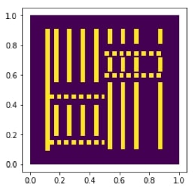
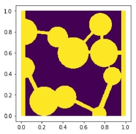
Figure 1: (a)The profile of $\kappa^{-1}$ in Example 3; (b) The profile of $\kappa^{-1}$ in Example 4.

Examples 3 and 4 do not have analytical solutions, so we do not list the convergence order as shown in the first two examples. We mention that the similar test of the profile of $\kappa^{-1}$ can be found in other literature [36, 43]. In the following two examples, a mesh $100\times 100$ is used and the data setting is designed as follows: $\Omega=(0,1)\times(0,1)$, $\bm{f}=\bm{0}$, $\nu=10^{-2}$ and $\bm{g}=(1,0)^{t}$. The Brinkman problems (3.13) are solved in a region with different contrast permeability.

Example 3.

For this test case, the profile of $\kappa^{-1}$ is plotted in Figure 1 with $\kappa^{-1}=10,10^{3},10^{5}$ in yellow region and $\kappa^{-1}=1$ in the purple region. ([43]).

For $\kappa^{-1}=10,10^{3},10^{5}$ in the yellow region and $\kappa^{-1}=1$ in purple region of 1, the first and the second components of the velocity obtained by MDG method with $\underline{\bm{\mathcal{P}}}^{\mathbb{S}}_{2}$-$\bm{\mathcal{P}}_{1}$ element are presented in Figure 2 and Figure 3, respectively. The stress intensity and pressure profiles are showed in Figure 4 and Figure 5.

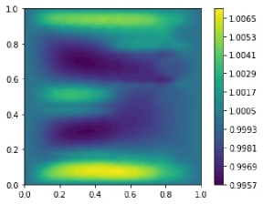
(a) $\kappa^{-1}=10$ in the yellow region

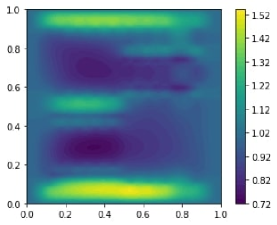
(b) $\kappa^{-1}=10^{3}$ in the yellow region

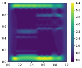
(c) $\kappa^{-1}=10^{5}$ in the yellow region

Figure 2: Distributions of $u_{1}$ with $\kappa^{-1}=1$ in purple region in Example 3.

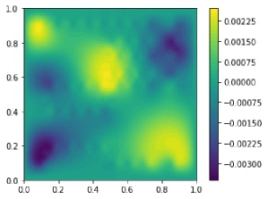
(a) $\kappa^{-1}=10$ in the yellow region

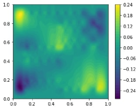
(b) $\kappa^{-1}=10^{3}$ in the yellow region

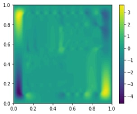
(c) $\kappa^{-1}=10^{5}$ in the yellow region

Figure 3: Distributions of $u_{2}$ with $\kappa^{-1}=1$ in purple region in Example 3.

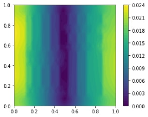
(a) $\kappa^{-1}=10$ in the yellow region

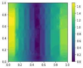
(b) $\kappa^{-1}=10^{3}$ in the yellow region

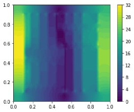
(c) $\kappa^{-1}=10^{5}$ in the yellow region

Figure 4: Distributions of $\underline{\bm{\sigma}}$ with $\kappa^{-1}=1$ in purple region in Example 3.

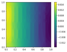
(a) $\kappa^{-1}=10$ in the yellow region

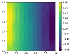
(b) $\kappa^{-1}=10^{3}$ in the yellow region

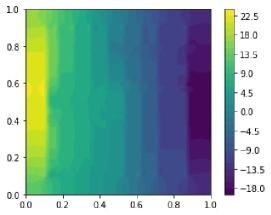
(c) $\kappa^{-1}=10^{5}$ in the yellow region

Figure 5: Distributions of $p$ with $\kappa^{-1}=1$ in purple region in Example 3.

Example 4.

In this example, the profile of $\kappa^{-1}$ is plotted in Figure 1 with $\kappa^{-1}=10,10^{3},10^{5}$ in the purple region and $\kappa^{-1}=1$ in yellow region. ([36, 43]).

For $\kappa^{-1}=10,10^{3},10^{5}$ in the purple region and $\kappa^{-1}=1$ in yellow region of 1, the first and the second components of the velocity obtained by MDG method with $\underline{\bm{\mathcal{P}}}^{\mathbb{S}}_{2}$-$\bm{\mathcal{P}}_{1}$ element are presented in Figure 6 and Figure 7, respectively. The stress intensity and pressure profiles are showed in Figure 8 and Figure 9.

From Figure 2 and Figure 3, we can see that the velocity of fluid in the purple region is faster and in the yellow region become slower as the contrast permeability increases. While, from Figure 6 and Figure 7, we can see that the velocity of fluid in the yellow region become faster and in the purple region become slower with the contrast permeability increasing. Figure 8 and Figure 9 show that the high contrast permeability gives rise to the large velocity difference, and the intensity and pressure increase rapidly.

Both Example 3 and Example 4 indicate that the contrast permeability is higher, the change of the velocity, pressure, and stress is greater. And they show the robustness, accuracy, and flexibility of the MDG method for the Brinkman problem.

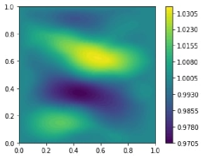
(a) $\kappa^{-1}=10$ in the purple region

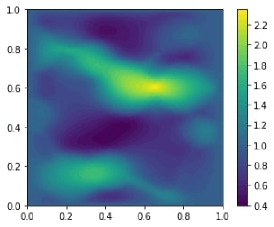
(b) $\kappa^{-1}=10^{3}$ in the purple region

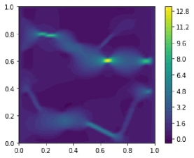
(c) $\kappa^{-1}=10^{5}$ in the purple region

Figure 6: Distributions of $u_{1}$ with $\kappa^{-1}=1$ in yellow region in Example 4.

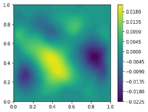
(a) $\kappa^{-1}=10$ in the purple region

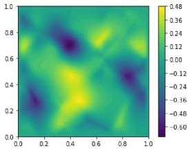
(b) $\kappa^{-1}=10^{3}$ in the purple region

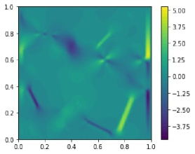
(c) $\kappa^{-1}=10^{5}$ in the purple region

Figure 7: Distributions of $u_{2}$ with $\kappa^{-1}=1$ in yellow region in Example 4.

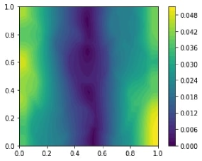
(a) $\kappa^{-1}=10$ in the purple region

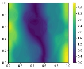
(b) $\kappa^{-1}=10^{3}$ in the purple region

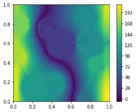
(c) $\kappa^{-1}=10^{5}$ in the purple region

Figure 8: Distributions of $\underline{\bm{\sigma}}$ with $\kappa^{-1}=1$ in yellow region in Example 4.

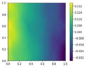
(a) $\kappa^{-1}=10$ in the purple region

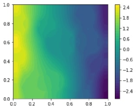
(b) $\kappa^{-1}=10^{3}$ in the purple region

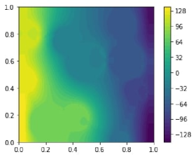
(c) $\kappa^{-1}=10^{5}$ in the purple region

Figure 9: Distributions of $p$ with $\kappa^{-1}=1$ in yellow region in Example 4.

6 Summary

In this paper, the mixed discontinuous Galerkin method with $\underline{\bm{\mathcal{P}}}^{\mathbb{S}}_{k+1}$-$\bm{\mathcal{P}}_{k}$ element pair is constructed and studied for solving the Brinkman equations based on the pseudostress-velocity formulation. The well-posedness of the MDG scheme is proved by the generalized Brezzi theory, and a priori error analysis is established. For any $k\geq 0$, we prove the optimal convergence order for the stress in broken $\underline{\bm{H}}(\mathbf{div})$ norm and velocity in $\bm{L}^{2}$ norm. Furthermore, the $\underline{\bm{L}}^{2}$ error estimate for the pseudostress is also investigated under certain conditions. Numerical examples confirm the theoretical results. In summary, the proposed MDG method for Brinkman equation has following main advantages: (i) it is uniformly stable and efficient from the Darcy limit to the Stokes limit; (ii) it provides accurate approximation to both the symmetric stress and the velocity; (iii) it is locally conservative for the physical quantities.

Acknowledgments. We thank Professor Suchuan Dong (Purdue University) for the helpful discussions.

References

- Aizinger et al. [2018] Aizinger, V., Rupp, A., Schütz, J., Knabner, P., 2018. Analysis of a mixed discontinuous Galerkin method for instationary Darcy flow. Comput. Geosci. 22 (1), 179–194.
- Arnold et al. [2002] Arnold, D. N., Brezzi, F., Cockburn, B., Marini, L. D., 2002. Unified analysis of discontinuous Galerkin methods for elliptic problems. SIAM J. Numer. Anal. 39 (5), 1749–1779.
- Arnold et al. [1984a] Arnold, D. N., Brezzi, F., Fortin, M., 1984a. A stable finite element for the Stokes equations. Calcolo 21 (4), 337–344 (1985).
- Arnold et al. [1984b] Arnold, D. N., Douglas, Jr., J., Gupta, C. P., 1984b. A family of higher order mixed finite element methods for plane elasticity. Numer. Math. 45 (1), 1–22.
- Barrios et al. [2012] Barrios, T. P., Bustinza, R., García, G. C., Hernández, E., 2012. On stabilized mixed methods for generalized Stokes problem based on the velocity-pseudostress formulation: a priori error estimates. Comput. Methods Appl. Mech. Engrg. 237/240, 78–87.
- Bassi and Rebay [1997] Bassi, F., Rebay, S., 1997. A high-order accurate discontinuous finite element method for the numerical solution of the compressible Navier-Stokes equations. J. Comput. Phys. 131 (2), 267–279.
- Behr et al. [1993] Behr, M. A., Franca, L. P., Tezduyar, T. E., 1993. Stabilized finite element methods for the velocity-pressure-stress formulation of incompressible flows. Comput. Methods Appl. Mech. Engrg. 104 (1), 31–48.
- Bey et al. [1995] Bey, K. S., Patra, A., Oden, J. T., 1995. -version discontinuous Galerkin methods for hyperbolic conservation laws: a parallel adaptive strategy. Internat. J. Numer. Methods Engrg. 38 (22), 3889–3908.
- Boffi et al. [2013] Boffi, D., Brezzi, F., Fortin, M., 2013. Mixed finite element methods and applications. Vol. 44 of Springer Series in Computational Mathematics. Springer, Heidelberg.
- Botti et al. [2018] Botti, L., Di Pietro, D. A., Droniou, J., 2018. A Hybrid High-Order discretisation of the Brinkman problem robust in the Darcy and Stokes limits. Comput. Methods Appl. Mech. Engrg. 341, 278–310.
- Braack and Schieweck [2011] Braack, M., Schieweck, F., 2011. Equal-order finite elements with local projection stabilization for the Darcy-Brinkman equations. Comput. Methods Appl. Mech. Engrg. 200 (9-12), 1126–1136.
- Brenner et al. [2012] Brenner, S. C., Sung, L.-Y., Zhang, H., Zhang, Y., 2012. A quadratic interior penalty method for the displacement obstacle problem of clamped Kirchhoff plates. SIAM J. Numer. Anal. 50 (6), 3329–3350.
- Brezzi et al. [1987] Brezzi, F., Douglas, Jr., J., Durán, R., Fortin, M., 1987. Mixed finite elements for second order elliptic problems in three variables. Numer. Math. 51 (2), 237–250.
- Brezzi et al. [1985] Brezzi, F., Douglas, Jr., J., Marini, L. D., 1985. Two families of mixed finite elements for second order elliptic problems. Numer. Math. 47 (2), 217–235.
- Brezzi and Fortin [1991] Brezzi, F., Fortin, M., 1991. Mixed and hybrid finite element methods. Vol. 15 of Springer Series in Computational Mathematics. Springer-Verlag, New York.
- Brezzi et al. [2005] Brezzi, F., Hughes, T. J. R., Marini, L. D., Masud, A., 2005. Mixed discontinuous Galerkin methods for Darcy flow. J. Sci. Comput. 22/23, 119–145.
- Brezzi et al. [2000] Brezzi, F., Manzini, G., Marini, D., Pietra, P., Russo, A., 2000. Discontinuous Galerkin approximations for elliptic problems. Numer. Methods Partial Differential Equations 16 (4), 365–378.
- Brinkman [1949] Brinkman, H., 1949. A calculation of the viscous force exerted by a flowing fluid on a dense swarm of particles. Flow Turbul. Combust. 1 (1), 27–34.
- Burman and Hansbo [2005] Burman, E., Hansbo, P., 2005. Stabilized Crouzeix-Raviart element for the Darcy-Stokes problem. Numer. Methods Partial Differential Equations 21 (5), 986–997.
- Cáceres et al. [2017] Cáceres, E., Gatica, G. N., Sequeira, F. A., 2017. A mixed virtual element method for the Brinkman problem. Math. Models Methods Appl. Sci. 27 (4), 707–743.
- Cai et al. [2010] Cai, Z., Tong, C., Vassilevski, P. S., Wang, C., 2010. Mixed finite element methods for incompressible flow: stationary Stokes equations. Numer. Methods Partial Differential Equations 26 (4), 957–978.
- Chen and Shu [2017] Chen, T., Shu, C.-W., 2017. Entropy stable high order discontinuous Galerkin methods with suitable quadrature rules for hyperbolic conservation laws. J. Comput. Phys. 345, 427–461.
- Cockburn et al. [2000] Cockburn, B., Karniadakis, G. E., Shu, C.-W., 2000. Discontinuous Galerkin methods. Vol. 11 of Lecture Notes in Computational Science and Engineering. Springer-Verlag, Berlin.
- Crouzeix and Raviart [1973] Crouzeix, M., Raviart, P.-A., 1973. Conforming and nonconforming finite element methods for solving the stationary Stokes equations. I. Rev. Française Automat. Informat. Recherche Opérationnelle Sér. Rouge 7 (R-3), 33–75.
- Farhloul and Fortin [1993] Farhloul, M., Fortin, M., 1993. A new mixed finite element for the Stokes and elasticity problems. SIAM J. Numer. Anal. 30 (4), 971–990.
- Gatica et al. [2014] Gatica, G. N., Gatica, L. F., Márquez, A., 2014. Analysis of a pseudostress-based mixed finite element method for the Brinkman model of porous media flow. Numer. Math. 126 (4), 635–677.
- Gatica et al. [2010] Gatica, G. N., Márquez, A., Sánchez, M. A., 2010. Analysis of a velocity-pressure-pseudostress formulation for the stationary Stokes equations. Comput. Methods Appl. Mech. Engrg. 199 (17-20), 1064–1079.
- Gatica and Sequeira [2015] Gatica, G. N., Sequeira, F. A., 2015. Analysis of an augmented HDG method for a class of quasi-Newtonian Stokes flows. J. Sci. Comput. 65 (3), 1270–1308.
- Gatica and Sequeira [2018] Gatica, L. F., Sequeira, F. A., 2018. A priori and a posteriori error analyses of an HDG method for the Brinkman problem. Comput. Math. Appl. 75 (4), 1191–1212.
- Gong et al. [2019] Gong, S., Wu, S., Xu, J., 2019. New hybridized mixed methods for linear elasticity and optimal multilevel solvers. Numer. Math. 141 (2), 569–604.
- Guzmán and Scott [2019] Guzmán, J., Scott, L. R., 2019. The Scott-Vogelius finite elements revisited. Math. Comp. 88 (316), 515–529.
- Hong et al. [2019] Hong, Q., Wang, F., Wu, S., Xu, J., 2019. A unified study of continuous and discontinuous Galerkin methods. Sci. China Math. 62 (1), 1–32.
- Hu [2015] Hu, J., 2015. Finite element approximations of symmetric tensors on simplicial grids in : the higher order case. J. Comput. Math. 33 (3), 283–296.
- Hu and Zhang [2014] Hu, J., Zhang, S., 2014. A family of conforming mixed finite elements for linear elasticity on triangular grids. arXiv:1406.7457.
- Hu and Zhang [2015] Hu, J., Zhang, S., 2015. A family of symmetric mixed finite elements for linear elasticity on tetrahedral grids. Sci. China Math. 58 (2), 297–307.
- Iliev et al. [2011] Iliev, O., Lazarov, R., Willems, J., 2011. Variational multiscale finite element method for flows in highly porous media. Multiscale Model. Simul. 9 (4), 1350–1372.
- Juntunen and Stenberg [2010] Juntunen, M., Stenberg, R., 2010. Analysis of finite element methods for the Brinkman problem. Calcolo 47 (3), 129–147.
- Kaya and Rivière [2005] Kaya, S., Rivière, B., 2005. A discontinuous subgrid eddy viscosity method for the time-dependent Navier-Stokes equations. SIAM J. Numer. Anal. 43 (4), 1572–1595.
- Könnö and Stenberg [2011] Könnö, J., Stenberg, R., 2011. -conforming finite elements for the Brinkman problem. Math. Models Methods Appl. Sci. 21 (11), 2227–2248.
- Langtangen and Logg [2016] Langtangen, H. P., Logg, A., 2016. Solving PDEs in Python. Vol. 3 of Simula SpringerBriefs on Computing. Springer, Cham.
- Ligaarden et al. [2010] Ligaarden, I., Krotkiewski, M., Lie, K.-A., Pal, M., Schmid, D., 2010. On the Stokes-Brinkman equations for modeling flow in carbonate reservoirs. In: ECMOR XII-12th European Conference on the Mathematics of Oil Recovery. Vol. September, 6–9 of Lect. Notes Comput. Sci. Eng. Oxford, UK.
- Mardal et al. [2002] Mardal, K. A., Tai, X.-C., Winther, R., 2002. A robust finite element method for Darcy-Stokes flow. SIAM J. Numer. Anal. 40 (5), 1605–1631.
- Mu et al. [2014] Mu, L., Wang, J., Ye, X., 2014. A stable numerical algorithm for the Brinkman equations by weak Galerkin finite element methods. J. Comput. Phys. 273, 327–342.
- Raviart and Thomas [1977] Raviart, P.-A., Thomas, J. M., 1977. A mixed finite element method for 2nd order elliptic problems, 292–315. Lecture Notes in Math., Vol. 606.
- Scott and Vogelius [1985] Scott, L. R., Vogelius, M., 1985. Norm estimates for a maximal right inverse of the divergence operator in spaces of piecewise polynomials. RAIRO Modél. Math. Anal. Numér. 19 (1), 111–143.
- Scott and Zhang [1990] Scott, L. R., Zhang, S., 1990. Finite element interpolation of nonsmooth functions satisfying boundary conditions. Math. Comp. 54 (190), 483–493.
- Vafai [2010] Vafai, K., 2010. Porous media: applications in biological systems and biotechnology. Springer Series in Computational Mathematics. CRC Press, USA.
- Wang et al. [2014] Wang, F., Han, W., Cheng, X., 2014. Discontinuous Galerkin methods for solving a quasistatic contact problem. Numer. Math. 126 (4), 771–800.
- Wang et al. [2010] Wang, F., Han, W., Cheng, X.-L., 2010. Discontinuous Galerkin methods for solving elliptic variational inequalities. SIAM J. Numer. Anal. 48 (2), 708–733.
- Wang et al. [2019] Wang, F., Wu, S., Xu, J., 2019. A mixed discontinuous Galerkin method for linear elasticity with strongly imposed symmetry. arXiv:1902.08717.
- Wehrspohn [2005] Wehrspohn, R. B., 2005. Ordered porous nanostructures and applications. Springer Series in Computational Mathematics. Springer, New York.
- Wu et al. [2017] Wu, S., Gong, S., Xu, J., 2017. Interior penalty mixed finite element methods of any order in any dimension for linear elasticity with strongly symmetric stress tensor. Math. Models Methods Appl. Sci. 27 (14), 2711–2743.
- Zhai et al. [2016] Zhai, Q., Zhang, R., Mu, L., 2016. A new weak Galerkin finite element scheme for the Brinkman model. Commun. Comput. Phys. 19 (5), 1409–1434.