A GREEDY ALGORITHM FOR SPARSE PRECISION MATRIX APPROXIMATION

Abstract

Precision matrix estimation is an important problem in statistical data analysis. This paper introduces a fast sparse precision matrix estimation algorithm, namely GISS^ρ, which is originally introduced for compressive sensing. The algorithm GISS^ρ is derived based on $l_{1}$ minimization while with the computation advantage of greedy algorithms. We analyze the asymptotic convergence rate of the proposed GISS^ρ for sparse precision matrix estimation and sparsity recovery properties with respect to the stopping criteria. Finally, we numerically compare GISS^ρ to other sparse recovery algorithms, such as ADMM and HTP in three settings of precision matrix estimation. The numerical results show the advantages of the proposed algorithm.

Keywords Precision matrix estimation, CLIME estimator, sparse recovery, inverse scale space method, greedy methods.

1 Introduction

Covariance matrix and precision matrix estimation are two important problems in statistics analysis and data science. The problems become more challenging in high-dimensional setting where the number of variable dimension $p$ is larger than the sample size $n$, hence the need for a fast, accurate and stable precision/covariance matrix estimation is necessary. In the high-dimensional setting, classical methods and theoretical results with fixed $p$ and large $n$ are no longer applicable. Another huge challenge due to high dimension is high computational cost. Therefore, effective model and method are urgent facing high-dimensional data challenge.

Denote $\bm{X}=(X_{1},X_{2},\cdots,X_{p})^{T}$ by a $p$ variate random vector. The covariance matrix and precision matrix can be traditionally denoted by $\Sigma_{0}$ and $\Omega_{0}=\Sigma^{-1}_{0}$ respectively. Assume an independent and identically distributed $n$ random samples $\{\bm{X}_{1},\bm{X}_{2},\cdots,\bm{X}_{n}\}$ are from the distribution of $\bm{X}$. The sample covariance matrix is the common method among the estimators of covariance matrix, which is defined as follows,

$$\Sigma_{n}=\frac{1}{n-1}\sum_{k=1}^{n}(\bm{X}_{k}-\bar{\bm{X}})(\bm{X}_{k}-\bar{\bm{X}})^{T}$$

where $\bar{\bm{X}}=\frac{1}{n}\sum_{k=1}^{n}\bm{X}_{k}$ denotes the sample mean. When $p$ is larger than $n$, it is obvious that $\Sigma_{n}$ is singular and the estimation for $\Omega_{0}$ naturally becomes unstable and imprecise.

Estimation of precision matrix in high-dimensional setting has been studied for a long time. For example, when the random variable $\bm{X}$ follows a certain ordering structure, methods based on banding the Cholesky factor of the inverse of sample covariance matrix were studied in [37, 2]. Penalized likelihood methods such as $l_{1}$-MLE type estimators were studied in [21, 14, 40] and the convergence rate in Frobenius norm was given by [34]. In [39], the authors established the convergence rate for sub-Gaussian distribution cases. For more restrictive conditions, such as mutual incoherence or irrepresentable conditions, [33] showed the convergence rates in elementwise $l_{\infty}$ norm and spectral norm. To overcome the drawbacks that $l_{1}$ penalty inevitably leads to biased estimation, nonconvex penalty such as SCAD penalty [24, 17] was proposed [18, 43], although it often requires high computational cost.

Recently, [11] proposed a new constrained $l_{1}$ minimization approach called CLIME for sparse precision estimation. Convergence rates in spectral norm, elementwise $l_{\infty}$ norm and Frobenius norm were established under weaker assumptions and shown to be faster than those $l_{1}$-MLE estimators when the population distributions have polynomial-type tails. In addition, CLIME provides an effective computational performance as the columns of precision matrix estimation can be independently obtained and accelerated by parallelized computing. However, in [11], each column is obtained by a solving a linear programming, which could be still time-consuming for high dimension. More efficient approach are still needed to be developed for practical high dimensional applications.

In compressive sensing and sparse optimization community, many algorithms and related theoretical results are developed for $l_{1}$ minimization optimization problems [1, 6, 7, 23, 30, 38, 41]. Greedy inverse scale space flows (GISS) [27], originally stems from the adaptive inverse scale (aISS) method [5], is a new sparse recovery approach combining the idea of greedy approach and $\ell_{1}$ minimization. The advantage of GISS method was efficiency compared to the aISS method. GISS^ρ with $\rho$ being an acceleration factor, as a variant of GISS, can further accelerate sparse solution recovery by increasing the support of the current iterate by many indices at once.

In this article, we take the advantages of CLIME estimator framework and GISS^ρ algorithm and propose a new efficient approach for sparse precision matrix estimation. More specifically, we transfer the the constraint bound in CLIME estimator to a turning parameter in the stop criteria in GISS^ρ method. Convergence result in elementwise $l_{\infty}$ norm is established under weaker assumptions same as [11]. Moreover, under the Gaussian noise setting, the stopping time based on the data term is also obtained. The numerical experiments shows the competitive advantage of computation time, on obtaining the same level of sparsity and accuracy compared to other existing methods.

The rest of the paper is organized as follows. In Section 2, we firstly introduce basic notations and simply revisit the CLIME estimator. In Section 3, we present the basic idea of our new method derived from CLIME estimator and GISS^ρ algorithm. In Section 4, we establish the theoretical analysis with assumptions. Section 5 presents the numerical results including simulated experiments and application on real data. We provide the discussion and conclusion in Section 6 and the proof of the main results can be found in Appendix.

2 Preliminary

2.1 Notations and definitions

Before presenting our proposed precision matrix estimator, we first introduce some essential notations and definitions.

For a vector $\bm{a}=(a_{1},a_{2},\ldots,a_{n})^{T}\in\mathbb{R}^{n}$, we define $|\bm{a}|_{1}=\sum_{j=1}^{n}|a_{j}|$, $|\bm{a}|_{2}=\sqrt{\sum_{j=1}^{n}a_{j}^{2}}$ and $|\bm{a}|_{\infty}=\mathrm{max}_{1\leq j\leq n}~{}|a_{j}|$ to denote the vector norms. Define the two types of inner products between two vectors by $\langle\bm{a},\bm{b}\rangle=\bm{a}^{T}\bm{b}$ and $\langle\bm{a},\bm{b}\rangle_{n}=\frac{1}{n}\bm{a}^{T}\bm{b}$, and denote $\|\bm{\bm{a}}\|_{n}=\frac{1}{\sqrt{n}}|\bm{a}|_{2}$.

For a matrix $\bm{A}=(a_{ij})\in\mathbb{R}^{p\times p}$, we define the elementwise $l_{\infty}$ norm $|\bm{A}|_{\infty}=\mathrm{max}_{1\leq i\leq p,1\leq j\leq p}|a_{ij}|$, the spectral norm $\|\bm{A}\|_{2}=\mathrm{sup}_{|\bm{x}|_{2}\leq 1}|\bm{Ax}|_{2}$, the $L_{1}$ norm $\|\bm{A}\|_{L_{1}}=\mathrm{max}_{1\leq j\leq p}\sum_{i=1}^{p}|a_{ij}|$, the infinity norm $\|\bm{A}\|_{\infty}=\mathrm{max}_{1\leq i\leq p}\sum_{j=1}^{p}|a_{ij}|$, the Frobenius norm $\|\bm{A}\|_{F}=\sqrt{\sum_{i=1}^{p}\sum_{j=1}^{p}a_{ij}^{2}}$, and the elementwise $L_{1}$ norm $\|\bm{A}\|_{1}=\sum_{i=1}^{p}\sum_{j=1}^{p}|a_{ij}|$.

The $i$th row and $j$th column of the matrix $\bm{A}$ are denoted by $\bm{A}_{i,\cdot}$ and $\bm{A}_{\cdot,j}$ respectively and the transpose of $\bm{A}$ is denoted by $\bm{A}^{T}$. Let $\bm{A}^{*}=\frac{1}{p}A^{T}$ denote the adjoint operator of $\bm{A}$ with respect to the inner product $\langle\cdot,\cdot\rangle_{p}$. The inner product between two matrix $\bm{A}$ and $\bm{B}$ is denoted by $\langle\bm{A},\bm{B}\rangle=\sum_{i}(\bm{A}^{T}\bm{B})_{ii}$ with proper size. For two index sets $T$ and $T^{\prime}$, we use $\bm{A}_{TT^{\prime}}$ to denote the $|T|\times|T^{\prime}|$ matrix with rows and columns of $\bm{A}$ indexed by $T$ and $T^{\prime}$ respectively and $\bm{A}\succ 0$ means that $\bm{A}$ is positive definite. It also should be noted the $p\times p$ identity matrix is defined by $I$ while $\mathbb{I}$ denoted the indicator function.

For two real sequences $\{\epsilon_{n}\}$ and $\{\eta_{n}\}$, we write $\epsilon_{n}=O(\eta_{n})$ if there exists a constant $C$ such that $|\epsilon_{n}|\leq C|\eta_{n}|$ for large $n$, $\epsilon_{n}=o(\eta_{n})$ if $\mathrm{lim}_{n\rightarrow\infty}{\epsilon_{n}}/{\eta_{n}}=0$.

2.2 CLIME estimator

The CLIME estimator in [11] proposed to obtain a precision matrix estimation via solving the following $l_{1}$ minimization:

min $$\|{\Omega}\|_{1}$$ (1)

s.t $$|\Sigma_{n}{\Omega}-I|_{\infty}\leq\lambda_{n},\;{\Omega}\in\mathbb{R}^{p\times p}$$

where $\Sigma_{n}\in\mathbb{R}^{p\times p}$ is the sample covariance matrix generated by $n$ data samples, $\Omega$ is the precision matrix to be estimated and the turning parameter $\lambda_{n}$ is set for controlling the approximation error under the elementwise $l_{\infty}$ norm.

In general, the solution $\hat{\Omega}_{1}=(\omega_{ij})$ of (1) is asymmetric, hence a symmetry strategy as followed was adopted in [11],

$$\hat{\Omega}=(\hat{\omega}_{ij}),\;\text{where}$$ (2)

$$\hat{\omega}_{ij}=\hat{\omega}_{ji}={\omega}_{ij}~{}\mathbb{I}(|\omega_{ij}|\leq|\omega_{ji}|)+{\omega}_{ji}~{}\mathbb{I}(|\omega_{ij}|>|\omega_{ji}|)\;\text{for}\;i,j=1,2,\cdots,p.$$

The above defined $\hat{\Omega}$ is the final estimated precision matrix through CLIME estimator.

It is easy to see that the convex program (1) can be decomposed into the following $p$ vector convex minimization problems:

min $$|\bm{\beta_{i}}|_{1}$$ (3)

s.t. $$|\Sigma_{n}\bm{\beta_{i}}-\bm{e_{i}}|_{\infty}\leq\lambda_{n},\;\beta_{i}\in\mathbb{R}^{p},$$

for all $1\leq i\leq p$, where $\bm{e_{i}}$ is a standard unit vector in $\mathbb{R}^{p}$. Denote $\hat{\bm{\beta_{i}}}$ as the solution of (3), then the assembling of the $p$ vectors in the form of $[\hat{\bm{\beta}}_{1},\hat{\bm{\beta}}_{2},\cdots,\hat{\bm{\beta}}_{p}]$ is a solution of (1), and vice visa.

For the case that the covariance matrix $\Sigma_{n}$ is not invertible, we can also consider a regularized

$$\Sigma_{n,\gamma} =\Sigma_{n}+\gamma I$$ (4)

for $\gamma>0$. Our GISS^ρ estimator can be obtained via solving the following minimization problem:

min $$|\bm{\beta_{i}}|_{1}$$ (5)

s.t. $$\Sigma_{n,\gamma}\bm{\beta_{i}}=\bm{e_{i}},\;\bm{\beta_{i}}\in\mathbb{R}^{p}$$

for all $1\leq i\leq p$ with the $l_{\infty}$ norm stopping criterion $i.e.$ $|\Sigma_{n,\gamma}\bm{\beta_{i}}-\bm{e_{i}}|_{\infty}\leq\lambda_{n}$.

3 Sparse precision matrix estimation by GISS^ρ

Before presenting the GISS^ρ estimator for sparse precision matrix, we first introduce the basic ideas of GISS and GISS^ρ. It stems from the adaptive inverse scale (aISS) method [5], which was firstly proposed for solving compressive sensing problem. In the following, we present the algorithms in the context of precision matrix estimation for the consistency of notations.

3.1 Inverse scale space (ISS) based algorithms

The aISS algorithm was proposed to solve the equality constrained $l_{1}$ minimization (basic pursuit) problem. In the context of precision matrix estimation, we consider

min $$|\bm{\beta}|_{1}$$ (6)

s.t. $$\Sigma\bm{\beta}=\bm{e}$$

where $\Sigma\in\mathbb{R}^{p\times p}$ denotes the covariance matrix, $\bm{\beta}\in\mathbb{R}^{p}$ represents one column of the sparse precision matrix to be reconstructed and $\bm{e}\in\mathbb{R}^{p}$ denotes one column of identity matrix $I$.

For the $l_{1}$ minimization optimization problem for a general matrix $\Sigma$ and vector $\bm{e}$, Bregman iteration (BI) and augmented Lagrangian (AL) method are two efficient equivalent iterative methods [29, 16, 38]. By applying BI to solve (6), we obtain the following iterative sequence:

$$\bm{\beta}^{k+1}=\mathrm{arg\ min}\ |\bm{\beta}|_{1}+\frac{\lambda}{2}|\Sigma\bm{\beta}-\bm{e}|_{2}^{2}-\langle\bm{p}^{k},\bm{\beta}\rangle,$$ (7a)

$$\bm{p}^{k+1}=\bm{p}^{k}+\lambda\Sigma^{T}(\bm{e}-\Sigma\bm{\beta}^{k+1}),$$ (7b)

where $k$ is the iteration step, $\bm{p}$ is the dual variable introduced in the optimization problem and $\lambda>0$ is step size for dual variable update.

In the above iterative scheme, the optimal condition of (7a) yields $\bm{p}^{k+1}\in\partial|\bm{\beta}^{k+1}|_{1}$ on combining with Equation (7b). Equation (7b) can be reformulated as

$$\frac{\bm{p}^{k+1}-\bm{p}^{k}}{\lambda}=\Sigma^{T}(\bm{e}-\Sigma\bm{\beta}^{k+1}).$$ (8)

If we consider both primal variable $\bm{\beta}$ and dual variable $\bm{p}$ as functions of time $t$ and interpret $\lambda$ as the time step, BI can be transformed into a dynamic equation:

$$\partial_{t}\bm{p}(t)=\Sigma^{T}(\bm{e}-\Sigma\bm{\beta}(t))$$ (9)

s.t $$\bm{p}(t)\in\partial|\beta(t)|_{1}.$$

The above differential inclusion is called inverse scale space flow (ISS) [4].

The main idea of aISS [5] is that the support of the solution $\bm{\beta}(t^{k})$ can be determined by the subgradient $\bm{p}(t^{k})$ at some time $t^{k}$ based on the following relation

$$\bm{p}\in\partial|\bm{\beta}|_{1}\Leftrightarrow\left\{\begin{array}[]{lll}\bm{p}_{i}=\mathrm{sign}(\bm{\beta}_{i}),&\mathrm{if}\ \bm{\beta}_{i}\neq 0,\\ |\bm{p}_{i}|\leq 1,&\mathrm{otherwise}.\end{array}\right.$$ (12)

for all $1\leq i\leq p$, i.e. the support of $\bm{\beta}(t^{k})$ is restricted onto the set $I=\{i\mid|\bm{p}_{i}(t^{k})|=1\}$. Furthermore, the step size $t^{k}$ can be determined as the change of the signal is piecewise linear, and the signal was obtained via solving a low dimensional optimization problem under the constraint of the sign consistence between $\bm{p}_{i}(t^{k})$ and $\bm{\beta}_{i}(t^{k})$.

3.2 GISS^ρ estimator

Motivated by the similarities between greedy algorithms (e.g. OMP [32, 26, 36], WOMP [35, 20], CoSaMP [28] and HTP [19]) and $l_{1}$ minimization algorithms (e.g. aISS), the authors in [27] proposed GISS method which approximates aISS flow closely. By removing the sign consistence constraint in aISS, GISS method achieves a more efficient scheme and provide a posterior method to estimate the distance to the $l_{1}$ minimizer. GISS method not only inherits remarkable properties from aISS, such as finite steps convergence but also shows much faster computation speed [27]. The modified version, namely GISS^ρ, can further accelerate the computation speed by including larger set of index with a factor $\rho\geq 1$.

Because of the efficiency of GISS^ρ algorithm for sparse recovery, we propose to apply it to estimate the columns of precision matrix, based on the formulation (1). More specifically, we propose GISS^ρ estimator by applying GISS^ρ algorithm via solving the following minimization problem:

min $$|\bm{\beta_{i}}|_{1}$$ (13)

s.t. $$\Sigma_{n}\bm{\beta_{i}}=\bm{e_{i}},\;\bm{\beta_{i}}\in\mathbb{R}^{p}$$

for all $1\leq i\leq p$ with the $l_{\infty}$ norm stopping criterion $i.e.$ $|\Sigma_{n}\bm{\beta_{i}}-\bm{e_{i}}|_{\infty}\leq\lambda_{n}$. The detail for solving each subproblem is shown in Algorithm 1.

Algorithm 1 GISS^ρ method.

Parameters: $\Sigma_{n},\ \bm{e_{i}},~{}\rho\geq 1,~{}\lambda_{n}\geq 0$
Initialization: $\bm{r_{0}}=\bm{e_{i}},t_{1}=1/|\Sigma_{n}^{T}\bm{r_{0}}|_{\infty},\ \bm{p}(t_{1})=t_{1}\Sigma_{n}^{T}\bm{r_{0}}$

while $|\bm{r_{k}}|_{\infty}>\lambda_{n}$ do

1. Compute $I_{k}=\{i\mid|\tilde{\bm{p}}_{i}(t_{k})|=1\}$

2. Compute $\bm{\beta}(t_{k})=\mathrm{arg\ min}_{\bm{\beta}}\{|\Sigma_{n}{P_{I_{k}}}\bm{\beta}-\bm{e}|_{2}^{2}\}$

3. Compute the residual $\bm{r_{k}}=\bm{e}-\Sigma_{n}\bm{\beta}(t^{k})$

4. Obtain $t_{k+1}$ as (3.1)    $t_{k+1}$ = $\rho$min{$t\ |\ t>t_{k},\exists j\mathrel{\mathop{\mathchar 58\relax}}|\bm{p}_{j}(t)|=1,\ \bm{\beta}_{j}(t_{k})=0,\ \bm{p}_{j}(t)\neq\bm{p}_{j}(t_{k})$},

where (3.2)    $\bm{p}_{j}(t)=\bm{p}_{j}(t_{k})+(t-t_{k})(\Sigma_{n}^{T}\bm{r_{k}})_{j}$

5. Update the dual variable $\bm{p}(t)$ via (3.2) with $t=t_{k+1}$ and $\tilde{\bm{p}}(t^{k+1})=$sign$(\bm{p}(t^{k+1}))$min$(|\bm{p}(t^{k+1})|,1)$

end while

return $\bm{\beta}(t_{k})$ as $\bm{\beta_{i}}$.

We note that as CLIME estimator, the estimation of each column can be performed in parallel. Also the difference between GISS^ρ estimator and CLIME estimator is the role of $\lambda_{n}$. More precisely, $\lambda_{n}$ in CLIME estimator is used as the model tolerance. By controlling the tuning parameter, CLIME estimator can explore broader region of the solution space and the optimization problem is solved by a primal dual interior point algorithm applied on the equivalent linear programming problem. For GISS^ρ estimator, $\lambda_{n}$ plays the role of the stopping criterion and the algorithm produces a sequence of estimators. As expected, from our observation, both in the theoretical analysis and simulation experiments, $\lambda_{n}$ shows similar results in GISS^ρ estimator comparing to CLIME estimator, while GISS^ρ estimator is more efficient, especially for large scale problem. The detailed numerical performance will be shown in Section 5.

4 Theoretical Analysis

4.1 Asymptotic analysis

In this section, we will present the asymptotic results of GISS^ρ estimator under standard moments conditions of the random variables. We denote the sample covariance matrix as $\textbf{$\Sigma_{n}$}=(\hat{\sigma}_{ij})=(\bm{\hat{\sigma}}_{1},\bm{\hat{\sigma}}_{2},\ldots,\bm{\hat{\sigma}}_{p})$, where $\bm{\hat{}}{\sigma}_{i},~{}i=1,\cdots,p$ are column vectors. The true covariance matrix as $\textbf{$\Sigma_{0}$}=(\sigma_{ij}^{0})$ and the expectation of a random variable (r.v.) $\bm{X}$ as E$\bm{X}=(\mu_{1},\ldots,\mu_{p})^{T}$. The following two cases are usually considered according to the moment conditions on $\bm{X}$.

(C1) Exponential-type tails: Suppose that there exist some $0\textless\eta\textless 1/4$ such that $\mathrm{log}p/n\leq\eta$ and

$$\mathrm{E}e^{t(X_{i}-\mu_{i})^{2}}\leq K\textless\infty\quad\mathrm{for\ all\ }|t|\leq\eta,\ \mathrm{for\ all\ }i,$$

where $K$ is a upper bounded constant.
(C2) Polynomial-type tails: Suppose that for some $\tilde{\gamma},\ c_{1}\textgreater 0,\ p\leq c_{1}n^{\tilde{\gamma}},$ and for some $\delta\textgreater 0$,

$$\mathrm{E}|X_{i}-\mu_{i}|^{4\tilde{\gamma}+4+\delta}\leq K\quad\mathrm{for\ all\ }i.$$

The following quantity is to measure the relation with the variance $\hat{\sigma}_{ij}$ which is useful in the theoretical property analysis,

$$\kappa=\mathrm{max}_{ij}~{}\mathrm{E}[(X_{i}-\mu_{i})(X_{j}-\mu_{j})-\sigma_{ij}^{0}]^{2}=\mathrel{\mathop{\mathchar 58\relax}}\mathrm{max}_{ij}~{}\kappa_{ij}.$$ (14)

The maximum value $\kappa$ captures the overall variability of $\Sigma_{n}$. With the condition (C1) and (C2), $\kappa$ is a bounded constant depending on $\tilde{\gamma},\delta,K$ [11].

Through the following convergence analysis, we consider the uniformity class of matrices to estimate the precision matrix $\Omega_{0}$,

$$U\mathrel{\mathop{\mathchar 58\relax}}=U(q,s_{0}(p))=\{\Omega\mathrel{\mathop{\mathchar 58\relax}}\Omega\succ 0,\;\|\Omega\|_{L_{1}}\leq M,\;\mathrm{max}_{1\leq i\leq p}\sum_{j=1}^{p}|\omega_{ij}|^{q}\leq s_{0}(p)\}$$

for $0\leq q<1$, where $\Omega=\mathrel{\mathop{\mathchar 58\relax}}(\omega_{ij})=(\bm{\omega}_{1},\bm{\omega}_{2},\cdots,\bm{\omega}_{p})$. For the special case $q=0$, $U(0,s_{0}(p))$ is a class of $s_{0}(p)$-sparse matrices.

Theorem 4.1.

Suppose that $\Omega_{0}\in U(q,s_{0}(p))$ and $\hat{\Omega}$ is the solution solved through GISS^ρ process with $\rho\geq 1$.

• Assume that (C1) holds. Let $\lambda_{n}=C_{0}M\sqrt{\frac{\mathrm{log}p}{n}}\textless\frac{1}{p}-\varrho$ for some $\varrho\textgreater 0$, where $C_{0}=2\eta^{-2}(2+\tau+\eta^{-1}e^{2}K^{2})^{2}$ and $\tau>0$. Then

  $$|\hat{\Omega}-\Omega_{0}|_{\infty}\leq C_{0}\left(3+\frac{1+3p\lambda_{n}}{1-p\lambda_{n}}\right)M^{2}\sqrt{\frac{\mathrm{log}p}{n}},$$ (15)

  with probability at least $1-4p^{-\tau}$.

• Assume that (C2) holds. Let $\lambda_{n}=D_{0}M\sqrt{\frac{\mathrm{log}p}{n}}\textless\frac{1}{p}-\varrho$ for some $\varrho\textgreater 0$, where $D_{0}=\sqrt{(5+\tau)(\kappa+1)}$. Then

  $$|\hat{\Omega}-\Omega_{0}|_{\infty}\leq D_{0}\left(3+\frac{1+3p\lambda_{n}}{1-p\lambda_{n}}\right)M^{2}\sqrt{\frac{\mathrm{log}p}{n}},$$ (16)

  with probability at least $1-O\left(n^{-\delta/8}+p^{-\tau/2}\right)$.

From the Theorem 4.1, we find that the convergence rate of our estimator is same to the one of CLIME estimator [11] in the sense of elementwise $l_{\infty}$ norm under two types of moment conditions, which consequently outperform $l_{1}$-MLE type estimators in the case of polynomial-type tails [33].

Similarly, we can obtain the following convergence results:

Theorem 4.2.

Suppose $\Omega_{0}\in U(q,s_{0}(p))$ and ($C1$) holds. Let $\lambda_{n}=C_{0}M\sqrt{\frac{\mathrm{log}p}{n}}\textless\frac{1}{p}-\varrho$ for some $\varrho\textgreater 0$ with $C_{0}$ defined in Theorem 4.1 and $\tau$ is sufficiently large. Let $\gamma=\sqrt{\frac{\mathrm{log}p}{n}}$. If $p\geq n^{\Xi}$ for some $\Xi\geq 0$. Then

$$\mathrm{sup}_{\Omega_{0}\in U}\mathrm{E}|\hat{\Omega}_{\gamma}-\Omega_{0}|^{2}_{\infty}=O\left(M^{4}\frac{\mathrm{log}p}{n}\right),$$ (17)

4.2 Sparsity recovery properties

In this subsection, we provide some analysis from the point of view of sparsity recovery in compressive sensing [35, 42, 15] as the original idea of GISS^ρ algorithm from the signal processing for the noisy free case. Since our method can be computed in the parallelism form, we consider only one column recovery of the precision for simplicity. Denote $\bm{r}=\hat{\Sigma}\bm{\beta}^{*}-\bm{e}$ where $\bm{e}\in\mathbb{R}^{p}$ stands for one column of the identity matrix ${I}_{p}$, $\hat{\Sigma}$ is the $p\times p$ sample or true covariance matrix and $\bm{\beta}^{*}$ is the related column of the precision matrix to be recovered. In the algorithm, the algorithm is stopped with the criteria $|\bm{r}|_{\infty}\leq\lambda_{n}$. In the above section, we have analyzed the convergence of the approximation in terms of $\lambda_{n}$. In this section, we will show two theoretical results on the sparsity recovery guarantee with the assumption that the residual is a gaussian random variable. More precisely, we analyze the setting that the linear operator as the covariance matrix or the approximation of covariance matrix as a linear operator, the columns of the precision matrix is the sparse vector to be recovered. The problem is reformulated as a sparse recovery problem as followed,

$$\bm{r}=\hat{\Sigma}\bm{\beta}^{*}-\bm{e}\sim N(\bm{0},\epsilon^{2}I_{p}).$$ (18)

The assumption of the residual or observation error is to be Gaussian with standard variation $\epsilon$. We assume that each $\bm{\beta}^{*}$ has less than $s\leq p$ nonzero components. For convenience, let $S$ = supp($\bm{\beta}^{*}$) be the support of the nonzero index set of $\bm{\beta^{*}}$ and $T$ be its complement set. $\hat{\Sigma}_{S}$ denotes the submatrix of $\hat{\Sigma}$ formed by the columns of $\hat{\Sigma}$ in $S$, which are assumed to be linearly independent. One can similarity define $\hat{\Sigma}_{T}$.

Before providing the sparsity recovery guarantee, we present necessary assumptions on the design matrix $i.e.$ covariance matrix $\hat{\Sigma}$.
(A1) Mutual Incoherence Condition:

$$\quad\mu\mathrel{\mathop{\mathchar 58\relax}}=\mathrm{max}_{i,j}\left|\frac{1}{p}\langle\hat{\Sigma}_{i},\hat{\Sigma}_{j}\rangle\right|\textless\frac{1}{2s-1},\quad s=|S|.$$

It can be shown [35, 5] that once A1 holds, then

$$\theta=1-\mu(s-1)$$

and

$$\vartheta=\frac{1-\mu(2s-1)}{1-\mu(s-1)}.$$

where $\theta$ and $\vartheta$ satisfies $\hat{\Sigma}_{S}^{*}\hat{\Sigma}_{S}\geq\theta I$ and $\|\hat{\Sigma}_{T}^{*}\hat{\Sigma}_{S}^{\dagger}\|_{\infty}\leq 1-\vartheta$ for $\hat{\Sigma}_{S}^{\dagger}\mathrel{\mathop{\mathchar 58\relax}}=\hat{\Sigma}_{S}(\frac{1}{p}\hat{\Sigma}_{S}^{T}\hat{\Sigma}_{S})^{-1}$ defined in Restricted Strong Convexity and Irrepresentable Conditions respectively. Moreover, the above two popular conditions can be verified with condition A1, while they are more difficult to be checked in practice [35, 5].

In the following, we will show that with large probability, the solution with the stopping rule $|\bm{r}|_{\infty}\leq\lambda_{n}$ recovers the true subset of the support index, under the assumption of Gaussian residual.

We further define the residual of the iterate $\bm{r}(t)=\bm{e}-\hat{\Sigma}\bm{\beta}(t)$ and then define the largest and the smallest nonzero magnitudes of $\bm{\beta}^{*}$ by $\bm{\beta}^{*}_{\mathrm{max}}\mathrel{\mathop{\mathchar 58\relax}}=\mathrm{max}(|\bm{\beta}_{i}^{*}|\mathrel{\mathop{\mathchar 58\relax}}i\in S)$ and $\bm{\beta}^{*}_{\mathrm{min}}\mathrel{\mathop{\mathchar 58\relax}}=\mathrm{min}(|\bm{\beta}_{i}^{*}|\mathrel{\mathop{\mathchar 58\relax}}i\in S)$ respectively.

The following Lemma show that the Gaussian noise is essentially bounded [10, 9].

Lemma 4.3.

For $\bm{r}\sim N(\bm{0},\epsilon^{2}I_{p})$ satisfies

$$P(\bm{r}\in B_{2})\geq 1-\frac{1}{p}$$ (19a)

$$P(\bm{r}\in B_{\infty}(\varsigma))\geq 1-\frac{1}{2p^{\varsigma}\sqrt{\pi\mathrm{log}p}}$$ (19b)

where $B_{2}=\left\{\bm{r}\mathrel{\mathop{\mathchar 58\relax}}|\bm{r}|_{2}\leq\epsilon\sqrt{p+2\sqrt{p\mathrm{log}p}}\right\}$ and $B_{\infty}(\varsigma)=\left\{\bm{r}\mathrel{\mathop{\mathchar 58\relax}}|\hat{\Sigma}^{T}\bm{r}|_{\infty}\leq\epsilon\sqrt{2(1+\varsigma)\mathrm{log}p}\right\}$ with $\varsigma>0$.

For the two essentially bounded cases, we have

Theorem 4.4.

Assume that (A1) holds and $\bm{r}\sim N(\bm{0},\epsilon^{2}I_{p})$, then

• For $l_{2}$ bounded Gaussian noise case (refer to (19a)),

  $$\bm{\beta}^{*}_{\mathrm{min}}\geq\frac{2\epsilon}{\sqrt{\theta}}\left(\sqrt{1+2\sqrt{\frac{\mathrm{log}p}{p}}}+\sqrt{\frac{\mathrm{log}s}{p}}\right)$$ (20)

  The GISS^ρ algorithm with the stopping rule $\|\bm{r}(t)\|_{\infty}\leq\epsilon\sqrt{1+2\sqrt{\frac{\mathrm{log}p}{p}}}$ selects the true subset of $S$ with probability at least $1-\frac{\mathrm{exp}{\left(-\frac{p}{2}+\frac{1}{2}\left(1+2\sqrt{\frac{\mathrm{log}p}{p}}\right)+\frac{p}{2}\mathrm{log}\left(2-\frac{1}{p}\left(1+2\sqrt{\frac{\mathrm{log}p}{p}}\right)\right)\right)}}{1-\frac{1}{p}\left(1+2\sqrt{\frac{\mathrm{log}p}{p}}\right)}-O(p^{-1})$.

• For $l_{\infty}$ bounded Gaussian noise case (refer to (19b)),

  $$\bm{\beta}^{*}_{\mathrm{min}}\geq\frac{2\epsilon\sqrt{\mathrm{max}_{i}\|\hat{\Sigma}_{i}\|_{p}(1+\varsigma)s\mathrm{log}p}}{{p\theta}\|\hat{\Sigma}\|_{L_{1}}}+2\epsilon\sqrt{\frac{\mathrm{log}s}{p\theta}}.$$ (21)

  The GISS^ρ with the stopping rule $\|\bm{r}(t)\|_{\infty}\leq 2\epsilon\|\hat{\Sigma}\|_{L_{1}}^{-1}{\sqrt{\mathrm{max}_{i}\|\hat{\Sigma}_{i}\|_{p}{(1+\varsigma)}\mathrm{log}p}}$ selects the true subset $S$ with probability at least $1-O(p^{-1})$.

Theorem 4.4 introduces a stopping rule with $l_{\infty}$ norm which only depends the residual level assumption and the conditions on $\beta^{*}_{\mathrm{min}}$ to ensure that all significant variables are selected [9].

5 Numerical Experiments

5.1 Experiments Setup

In the data simulation, we consider the following three cases.

• Case 1: Solve the sparse matrix with a designed covariance matrix: $\Sigma_{ij}=0.5^{|i-j|}$. The exact precision matrix $\Omega=\Sigma^{-1}$ is given as

  $$\Omega_{ij}=\left\{\begin{array}[]{lll}1.3333,&\mathrm{for}~{}i=j=1,p\\ 1.6667,&\mathrm{for}~{}1<i=j<p\\ -0.6667,&|i-j|=1\\ 0,&\mathrm{otherwise}.\end{array}\right.$$ (26)

• Case 2: The second simulation refers to [34]. Assume that the true precision matrix $\Omega=B+\delta I$, where each off-diagonal entry in $B$ is generated independently and equals 0.5 with probability 0.1 or 0 with probability 0.9. $\delta$ is chosen such that conditional number of $\Omega$ is equal to $p$ and the matrix is normalized to have the unit diagonals. Then we sample a set of data from the $p-$dimensional normal distribution $N(0,\Sigma)$ where $\Sigma=\Omega^{-1}$. The estimated covariance matrix from this set of generated data is used as $\Sigma_{n}$ for the recovery.

• Case 3: Application to the fMRI data for ADHD. Attention Deficit Hyperactivity Disorder (ADHD) is a mental disorder causing 5%-10% of school-age children in behavior controlling through the United States. The ADHD-200 project released a resting-state fMRI dataset of healthy controls and ADHD children for scientific research. The data we processed is from Kennedy Krieger Institute (KKI), one of participating centers. The preprocessing pipeline can be found in https://www.nitrc.org/plugins/mwiki/ index.php/neurobureau:AthenaPipeline. After preprocessing, we get 148 time points from each of 116 brain regions for each subject. We use the data of each subject to generate the sample covariance matrix for estimating the precision matrix which is similar to the methodology of numerical examples in [25].

The above three simulation setting are tested with different algorithms for a comparison to ours. The first one is Hard Thresholding Pursuit (HTP) proposed in  [19] for solving the basis pursuit problem similar to (13). The algorithm is a combination of the Iterative Hard Thresholding algorithm and the Compressive Sampling Matching Pursuit algorithm (Cosamp). The other algorithms that we draw into comparisons are based on $l_{1}$ regularizer, such as L1-magic  [12] and Alternating direction method of multipliers (ADMM) [3, 22, 13]. We denote $\text{ADMM}_{\lambda_{n}}$ for solving inequality constrained model (3) and ADMM for the equality constrained model (13) for comparison.

The computation time will be reported with a computation environment : MATLAB R2016b, Intel(R) Xeon(R) CPU E5-2689 v4 @3.10GHz.

5.2 Results

The result for Case 1 with different dimension $p$ is shown in the Table 1. The third column of the table shows the non-zero entries number of the different methods with the thresholding value $10^{-8}$ applied on the recovered precision matrix for those $l_{1}$ based methods. The third column shows the result with the thresholding value $10^{-4}$, as we find all the methods successfully recover the true support. The last two columns show the computation time and the relative error to the true solution in terms of Frobenius norm. We find that both our method GISS^ρ (here $\rho=1$) have good computation time performance, especially in the high dimensional settings.

Table 1: Case 1

Dimension	Algorithms	$L_{0}$ Norm (1e-8)	$L_{0}$ Norm (1e-4)	Time consuming (s)	Relative Error (Frobenius Norm)
200	GISS	598	598	0.1084	9.10e-10
	HTP	598		0.0826	9.10e-10
	L1-magic	1780		0.4679	1.00e-09
	$\text{ADMM}_{\lambda_{n}}$	1388		0.2649	8.14e-10
	ADMM	1390		0.2615	8.99e-10
400	GISS	1198	1198	0.1002	9.09e-10
	HTP	1198		0.0975	9.09e-10
	L1-magic	3580		2.7838	1.00e-09
	$\text{ADMM}_{\lambda_{n}}$	2788		1.5010	8.05e-10
	ADMM	2792		1.5014	8.98e-10
600	GISS	1798	1798	0.1479	9.09e-10
	HTP	1798		0.1567	9.09e-10
	L1-magic	5380		16.4614	1.04e-09
	$\text{ADMM}_{\lambda_{n}}$	4188		9.7355	8.02e-10
	ADMM	4192		10.4155	8.97e-10
800	GISS	2398	2398	0.2518	9.09e-10
	HTP	2398		0.3942	9.09e-10
	L1-magic	7180		113.4222	1.04e-09
	$\text{ADMM}_{\lambda_{n}}$	5588		36.3055	8.01e-10
	ADMM	5592		37.9462	8.97e-10
1000	GISS	2998	2998	0.4105	9.09e-10
	HTP	2998		0.7366	9.09e-10
	L1-magic	8980		392.0562	1.04e-09
	$\text{ADMM}_{\lambda_{n}}$	6988		74.3292	8.00e-10
	ADMM	6992		77.3578	8.97e-10
2000	GISS	5998	5998	2.4252	9.09e-10
	HTP	5998		5.4236	9.09e-10
	L1-magic	17980		6.1685e+03	1.04e-09
	$\text{ADMM}_{\lambda_{n}}$	13988		709.4917	7.98e-10
	ADMM	13992		733.7321	8.97e-10

For Case 2, we vary the dimension $p$ from $200$ to $600$ and replicate 20 times for each algorithms. We adopt 20 cores for a parallelization implementation for this case. In this numerical setting, we take $\rho=1.2,1.5,2.0>1$ in GISS^ρ for different $p$ and set 0.05 for the thresholding value. Table 2, 3, 4 and 5 show the averages errors (Mean) and standard errors (SE) of losses in terms of different matrix norms: Frobenius norm, $L_{1}$ norm, $L_{2}$ norm and elementwise $l_{\infty}$ norm. True positive (TP) number and True negative (TN) number are also computed. The last column is the average time consuming of each algorithm. For $p\geq n$ situation, we show the numerical results in Table 6 and 7 for $p=60,~{}100$ respectively. We set 0.01 for the thresholding value and we found the Frobenius norm results outperform other methods, although the SE are larger than others.

Table 2: Case 2, $p=200$, $\lambda_{200}$=$0.7\sqrt{\frac{\mathrm{log}p}{n}}$ with sample number $n$= 3000.

$p$=200	Frobenius norm	Matrix $L_{1}$ norm	Operator norm	$l_{\infty}$ Norm	Time consuming (s)
GISS	0.5457(0.008)	0.1084(0.016)	0.0125(0.003)	0.1314(0.003)	0.1219
HTP	0.2485(0.007)	0.0884(0.016)	0.0571(0.003)	0.1088(0.003)	0.3885
ADMM	0.3343(0.014)	0.2107(0.035)	0.0793(0.008)	0.1412(0.003)	0.1308
ADMM${}_{\lambda_{n}}$	1.2255(0.009)	0.5865(0.038)	0.2515(0.007)	0.1530(0.003)	0.4589

Table 3: Case 2, $p=400$, $\lambda_{400}$=$0.7\sqrt{\frac{\mathrm{log}p}{n}}$ with sample number $n$= 5000.

$p$=400	Frobenius norm	Matrix $L_{1}$ norm	Operator norm	$l_{\infty}$ Norm	Time consuming (s)
GISS	1.4850(0.011)	0.2796(0.028)	0.1253(0.004)	0.1478(0.002)	0.8004
HTP	0.4452(0.009)	0.1192(0.018)	0.1187(0.003)	0.1056(0.003)	6.3441
ADMM	0.9107(0.023)	0.1878(0.025)	0.1896(0.007)	0.1940(0.004)	0.8222
ADMM${}_{\lambda_{n}}$	2.0134(0.012)	0.5611(0.030)	0.3289(0.005)	0.1606(0.002)	8.4315

Table 4: Case 2, $p=600$, $\lambda_{600}$=$0.7\sqrt{\frac{\mathrm{log}p}{n}}$ with sample number $n$= 8000.

$p$=600	Frobenius norm	Matrix $L_{1}$ norm	Operator norm	$l_{\infty}$ Norm	Time consuming (s)
GISS	1.6309(0.010)	0.1536(0.022)	0.0171(0.003)	0.1290(0.001)	3.4359
HTP	0.4823(0.007)	0.2450(0.027)	0.2918(0.003)	0.0845(0.001)	43.1578
ADMM	2.1578(0.023)	0.3680(0.031)	0.0323(0.007)	0.1759(0.001)	12.7318
ADMM${}_{\lambda_{n}}$	2.2408(0.009)	0.5123(0.020)	0.2902(0.004)	0.1341(0.001)	13.6197

Table 5: Case 2, $p=200,~{}400,~{}600$.

	TP(%)			TN(%)
	200	400	600	200	400	600
GISS	99.93	98.43	94.29	99.71	99.93	100
HTP	99.95	97.95	92.35	99.81	99.99	100
ADMM	99.75	96.01	91.89	99.1	99.94	99.97
ADMM${}_{\lambda_{n}}$	99.97	99.09	96.52	98.69	99.84	99.99

Table 6: Case 2, $p=60$, $\lambda_{60}$=$0.001\sqrt{\frac{\mathrm{log}p}{n}}$ with sample number $n$= 30.

$p$=60	Frobenius norm	Matrix $L_{1}$ norm	Operator norm	$l_{\infty}$ Norm
GISS	1.3570(0.14)	3.8780(0.21)	1.1073(0.14)	1.4990(0.15)
HTP	8.4734(0.01)	2.8927(0.01)	2.2451(0.01)	0.8689(0.01)
ADMM	6.8352(0.00)	5.8557(0.02)	0.4718(0.00)	1.0770(0.01)
ADMM${}_{\lambda_{n}}$	6.8379(0.00)	5.8608(0.02)	0.4719(0.00)	1.0770(0.01)

Table 7: Case 2, $p=100$, $\lambda_{100}$=$0.001\sqrt{\frac{\mathrm{log}p}{n}}$ with sample number $n$= 50.

$p$=100	Frobenius norm	Matrix $L_{1}$ norm	Operator norm	$l_{\infty}$ Norm
GISS	1.6411(0.14)	5.1000(0.22)	0.9443(0.10)	1.4988(0.12)
HTP	11.2055(0.01)	4.1144(0.01)	2.7254(0.01)	0.9448(0.01)
ADMM	12.7463(0.00)	9.2365(0.02)	0.7048(0.00)	1.4200(0.01)
ADMM${}_{\lambda_{n}}$	12.7505(0.00)	9.2454(0.02)	0.7048(0.00)	1.4200(0.01)

In Theorem 4.1, we showed the convergence rate of the estimator with respect to the elementwise $l_{\infty}$ norm. From Figure 1, we can also numerically observe the linear convergence rate of $L_{2}$ norm and Frobenius norm, although this can not be shown theoretically in the current framework.

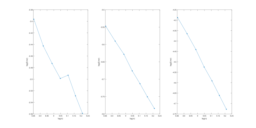
Figure 1: Error estimated through GISS^ρ algorithm (Left: Matrix elementwise $l_{\infty}$ norm; Middle: Operator norm; Right: Frobenius norm). We check the case in Model 2 when $p=400,~{}\rho=1$ and repeat the test for 20 times. The stopping criterion $\lambda_{n}$ is set as 0.05 and the sample number varies from 7000 to 10000.

For Case 3 where the real fMRI dataset for ADHD is used, we compare the performance of support recovery using the data from all subjects, and the results suggest that GISS^ρ has competitive performance with CLIME. Figure 2 compares the running time of GISS^ρ with different $\rho$, HTP algorithm, and $\text{ADMM}_{\lambda_{n}}$ algorithm. Similar to the procedure described before, for each subject, we use the each algorithm to recover a designated edge percentages: 10%, 20%, 30%, 40%, 50%. This plot shows that the running time of GISS^ρ grows quickly for $\rho=1$ when we need to recover more connections. However, when we change the value by taking $\rho$=2, we find both HTP and GISS^ρ ($\rho=2$) shows the similar performance. $\text{ADMM}_{\lambda_{n}}$ algorithm is the slowest among above three methods. We note that we omit the application of ADMM method to this dataset as the computation time performance is much worse than any other algorithms in Figure 2.

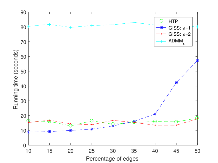
Figure 2: Comparison of running time for the ADHD dataset.

6 Discussion and Conclusion

This paper proposed a fast sparse algorithm GISS^ρ for estimating precision matrix, especially for the high dimensional problem setting. The GISS^ρ is a algorithm based on the $l_{1}$ minimization. However, it combines the advantage of the greedy algorithms. The asymptotic convergence and the sparse reovery properties of this algorithm are analyzed. Numerical simulations show that the proposed GISS^ρ estimator shows a good performance compared to HTP, ADMM and other $l_{1}$ based estimators, especially for high dimensional problems.

Appendix

Lemma 6.1.

Suppose that $\Omega_{0}\in U(q,s_{0}(p))$ and $\hat{\Omega}_{n,\gamma}$ is the solution solved by GISS^ρ for $\rho\geq 1$ and $\hat{\Sigma}_{n,\gamma}$ defined as (4) and symmetry operation defined in (2). If $\|\Omega_{0}\|_{L_{1}}(\mathrm{max}_{ij}|\hat{\sigma}_{ij}-\sigma_{ij}^{0}|+\gamma)\leq\lambda_{n}\leq\frac{1}{p}$, then we have

$$|\hat{\Omega}_{n,\gamma}-\Omega_{0}|_{\infty}\leq\left(3+{\frac{1+3p\lambda_{n}}{1-p\lambda_{n}}}\right)\lambda_{n}M,$$ (27)

where $C_{1}\leq 2(1+2^{1-q}+3^{1-q})\left(3M+{\frac{1+3p\lambda_{n}}{1-p\lambda_{n}}M}\right)^{1-q}$.

Proof.

According to the proof of Theorem 6 in [11], we denote $\hat{\Omega}_{n,\gamma}\mathrel{\mathop{\mathchar 58\relax}}=\hat{\Omega}_{\gamma}$. Let $\hat{\bm{\beta}}$ be the one column of $\Omega_{0}$ and the $\bm{\beta}$ be the final result of GISS^ρ estimator satisfying $|\Sigma_{n,\gamma}\bm{\beta}-\bm{e}|_{\infty}\leq\lambda_{n}$, then we have

$$|\Sigma_{0}(\hat{\bm{\beta}}-\bm{\beta})|_{\infty} \leq|\Sigma_{n,\gamma}(\hat{\bm{\beta}}-\bm{\beta})|_{\infty}+|(\Sigma_{n,\gamma}-\Sigma_{0})(\hat{\bm{\beta}}-\bm{\beta})|_{\infty}$$ (28a)

$$\leq|\Sigma_{n,\gamma}\hat{\bm{\beta}}-e|_{\infty}+|\Sigma_{n,\gamma}\bm{\beta}-e|_{\infty}+|\Sigma_{n,\gamma}-\Sigma_{0}|_{\infty}|\hat{\bm{\beta}}-\bm{\beta}|_{1}$$ (28b)

$$\leq|\Sigma_{n,\gamma}\hat{\bm{\beta}}-e|_{\infty}+\lambda_{n}+|\Sigma_{n,\gamma}-\Sigma_{0}|_{\infty}|\hat{\bm{\beta}}-\bm{\beta}|_{1}$$ (28c)

$$\leq|(\Sigma_{n,\gamma}-\Sigma_{0})\hat{\bm{\beta}}|_{\infty}+\lambda_{n}+|\Sigma_{n,\gamma}-\Sigma_{0}|_{\infty}|\hat{\bm{\beta}}-\bm{\beta}|_{1}$$ (28d)

$$\leq|\Sigma_{n,\gamma}-\Sigma_{0}|_{\infty}|\hat{\bm{\beta}}|_{1}+\lambda_{n}+|\Sigma_{n,\gamma}-\Sigma_{0}|_{\infty}|\hat{\bm{\beta}}-\bm{\beta}|_{1}$$ (28e)

$$\leq 2\lambda_{n}+|\Sigma_{n,\gamma}-\Sigma_{0}|_{\infty}|\hat{\bm{\beta}}-\bm{\beta}|_{1}$$ (28f)

$$\leq 2\lambda_{n}+|\Sigma_{n,\gamma}-\Sigma_{0}|_{\infty}(|\hat{\bm{\beta}}|_{1}+|\bm{\beta}|_{1})$$ (28g)

$$\leq 3\lambda_{n}+\frac{\lambda_{n}|\bm{\beta}|_{1}}{\|\Omega_{0}\|_{L_{1}}}$$ (28h)

Transform the result (28h) into matrix form and let $\hat{\Omega}^{1}_{\gamma}$ be the matrix form of $\beta$, it follows that

$$|\hat{\Omega}^{1}_{\gamma}-\Omega_{0}|_{\infty}\leq\|\Omega_{0}\|_{L_{1}}|\Sigma_{0}(\hat{\Omega}^{1}_{\gamma}-\Omega_{0})|_{\infty}\leq 3\lambda_{n}\|\Omega_{0}\|_{L_{1}}+{\lambda_{n}\|\hat{\Omega}^{1}_{\gamma}\|_{L_{1}}},$$ (29)

since

$$|AB|_{\infty}\leq\|A\|_{L_{1}}|B|_{\infty},$$ (30)

when $A$ is symmetric matrix.
Let $\tilde{\bm{p}}$ be the subgradient of $\|\cdot\|_{1}$ at $\bm{\beta}$, then

$$|\langle\tilde{\bm{p}},\hat{\bm{\beta}}-\bm{\beta}\rangle| \leq|\tilde{\bm{p}}|_{1}|\hat{\bm{\beta}}-\bm{\beta}|_{\infty}$$ (31a)

$$\leq p|\Omega_{0}\Sigma_{0}(\hat{\bm{\beta}}-\bm{\beta})|_{\infty}$$ (31b)

$$\leq p\|\Omega_{0}\|_{\infty}|\Sigma_{0}(\hat{\bm{\beta}}-\bm{\beta})|_{\infty}$$ (31c)

$${\color[rgb]{0,0,0}=p\|\Omega_{0}\|_{L_{1}}|\Sigma_{0}(\hat{\bm{\beta}}-\bm{\beta})|_{\infty}}$$ (31d)

$$\leq p\|\Omega_{0}\|_{L_{1}}\left(3\lambda_{n}+\frac{\lambda_{n}|\bm{\beta}|_{1}}{\|\Omega_{0}\|_{L_{1}}}\right)$$ (31e)

and since

$$|\hat{\bm{\beta}}|_{1}-|\bm{\beta}|_{1}-\langle\tilde{\bm{p}},\hat{\bm{\beta}}-\bm{\beta}\rangle\geq 0,$$ (32)

we have

$$|{\bm{\beta}}|_{1} \leq|\hat{\bm{\beta}}|_{1}-\langle\tilde{p},\hat{\bm{\beta}}-\bm{\beta}\rangle$$ (33a)

$$\leq|\hat{\bm{\beta}}|_{1}+p\|\Omega_{0}\|_{L_{1}}\left(3\lambda_{n}+\frac{\lambda_{n}|\bm{\beta}|_{1}}{\|\Omega_{0}\|_{L_{1}}}\right)$$ (33b)

In the matrix form, we have

$${\color[rgb]{0,0,0}\|\hat{\Omega}^{1}_{\gamma}\|_{L_{1}}\leq\|\Omega_{0}\|_{L_{1}}+3p\|\Omega_{0}\|_{L_{1}}\lambda_{n}+\lambda_{n}p\|\hat{\Omega}^{1}_{\gamma}\|_{L_{1}}}.$$ (34)

Therefore,

$${\color[rgb]{0,0,0}\|\hat{\Omega}^{1}_{\gamma}\|_{L_{1}}\leq\left(\frac{1+3p\lambda_{n}}{1-p\lambda_{n}}\right)\|\Omega_{0}\|_{L_{1}}}$$ (35)

Combining (35) and (29), we have

$${\color[rgb]{0,0,0}|\hat{\Omega}^{1}_{\gamma}-\Omega_{0}|_{\infty}\leq\|\Omega_{0}\|_{L_{1}}|\Sigma_{0}(\hat{\Omega}^{1}_{\gamma}-\Omega_{0})|_{\infty}\leq 3\lambda_{n}\|\Omega_{0}\|_{L_{1}}+{\lambda_{n}\left(\frac{1+3p\lambda_{n}}{1-p\lambda_{n}}\right)\|\Omega_{0}\|_{L_{1}}}}.$$ (36)

Following the symmetric operation of $\|\hat{\Omega}_{\gamma}\|_{L_{1}}$ introduced in (2), we have

$${\color[rgb]{0,0,0}|\hat{\Omega}_{\gamma}-\Omega_{0}|_{\infty}\leq|\hat{\Omega}^{1}_{\gamma}-\Omega_{0}|_{\infty}}.$$ (37)

This establishes (27) with (36). ∎

Combining the proof of Theorem 1(a) and 1(b) and Theorem 4(a), 4(b) in [11], Theorem 4.1 can be derived with Lemma 6.1. Similarly, Theorem 4.2 can be derived based on Theorem 2 and Theorem 5 in [11] and Lemma 6.1.

In the following, we prove the sparse recovery property Theorem 4.4.

Proof.

We first prove the first statement in Theorem 4.4. Following the proof of Theorem 6.1 and 6.2 in [31], the proof is divided into two parts. The first part shows that GISS^ρ will stop at the chosen stopping criteria with high probability and the second part is to assure the process will not stop if there still have supports to choose.

Let $b_{\infty}$ be the stopping point in the form of $l_{\infty}$ norm i.e. $b_{\infty}=\epsilon\sqrt{1+2\sqrt{\frac{\mathrm{log}p}{p}}}$. ${P}_{t}=\hat{\Sigma}_{S(t)}\left(\hat{\Sigma}^{*}_{S(t)}\hat{\Sigma}_{S(t)}\right)^{-1}\hat{\Sigma}_{S(t)}^{*}$. Obviously, $P_{t}$ is a symmetric projection matrix. It follows from Lemma 4 in [8], we have

$$\mathrm{Prob}(|\bm{r}(t)|_{\infty} =|(\textbf{I}-{P}_{t})\bm{\epsilon}|_{\infty}\geq b_{\infty})\leq\mathrm{Prob}(|\bm{\epsilon}|_{2}\geq b_{\infty})$$ (38a)

$$\leq\frac{1}{1-\frac{1}{p}\left(1+2\sqrt{\frac{\mathrm{log}p}{p}}\right)}\mathrm{exp}\left(-\frac{p}{2}\left(1-\frac{1}{p}\left(1+2\sqrt{\frac{\mathrm{log}p}{p}}\right)-\mathrm{log}\left(2-\frac{1}{p}\left(1+2\sqrt{\frac{\mathrm{log}p}{p}}\right)\right)\right)\right)$$ (38b)

$$=\frac{\mathrm{exp}{\left(-\frac{p}{2}+\frac{1}{2}\left(1+2\sqrt{\frac{\mathrm{log}p}{p}}\right)+\frac{p}{2}\mathrm{log}\left(2-\frac{1}{p}\left(1+2\sqrt{\frac{\mathrm{log}p}{p}}\right)\right)\right)}}{1-\frac{1}{p}\left(1+2\sqrt{\frac{\mathrm{log}p}{p}}\right)}$$ (38c)

which means the algorithm stops when the residual is less than $b_{\infty}$.
The following part is to show that the algorithm will not stop whenever there exits the $i\in S$ such that $\bm{\beta}_{i}^{*}(t)=0$. Similar to the proof of the Theorem 6.1 in [31], we have

$$|\bm{r}(t)|_{\infty} = |\hat{\Sigma}_{S}(\bm{\bm{\beta}}^{*}-\bm{\beta}_{S}(t))+(I-P_{S})\epsilon|_{\infty}$$ (39a)

$$\geq |\hat{\Sigma}_{S}(\bm{\beta}^{*}-\bm{\beta}_{S}(t))|_{\infty}-|(I-P_{S})\epsilon|_{\infty}$$ (39b)

$$\geq \sqrt{\theta}|\bm{\beta}^{*}-\bm{\beta}_{S}(t)|_{2}-b_{\infty}$$ (39c)

$$\geq \sqrt{\theta}\bm{\beta}^{*}_{\mathrm{min}}-b_{\infty}$$ (39d)

$$\geq b_{\infty}$$ (39e)

provided that ${\bm{\beta}}^{*}_{\mathrm{min}}\geq\frac{2\epsilon}{\sqrt{\theta}}\left(\sqrt{1+2\sqrt{\frac{\mathrm{log}p}{p}}}\right)$. Since

$$|(\hat{\Sigma}_{S}^{*}\hat{\Sigma}_{S})^{-1}\hat{\Sigma}_{S}^{*}\epsilon|_{\infty}\leq 2\epsilon\sqrt{\frac{\mathrm{log}s}{p\theta}},\ \ \mathrm{w}.\mathrm{p}.~{}\ \mathrm{at}\ \mathrm{least}\ 1-2p^{-1},$$ (40)

so it suffices to have

$$\bm{\beta}^{*}_{\mathrm{min}}\geq\frac{2\epsilon}{\sqrt{\theta}}\left(\sqrt{1+2\sqrt{\frac{\mathrm{log}p}{p}}}+\sqrt{\frac{\mathrm{log}s}{p}}\right).$$ (41)

∎

The second statement of Theorem 4.4 can be similarly proved.

References

- [1] A. Beck and M. Teboulle, “A fast iterative shrinkage-thresholding algorithm for linear inverse problems,” SIAM journal on imaging sciences, vol. 2, no. 1, pp. 183–202, 2009.
- [2] P. J. Bickel, E. Levina et al., “Covariance regularization by thresholding,” The Annals of Statistics, vol. 36, no. 6, pp. 2577–2604, 2008.
- [3] S. Boyd and L. Vandenberghe, Convex optimization. Cambridge university press, 2004.
- [4] M. Burger, G. Gilboa, S. Osher, J. Xu et al., “Nonlinear inverse scale space methods,” Communications in Mathematical Sciences, vol. 4, no. 1, pp. 179–212, 2006.
- [5] M. Burger, M. Möller, M. Benning, and S. Osher, “An adaptive inverse scale space method for compressed sensing,” Mathematics of Computation, vol. 82, no. 281, pp. 269–299, 2013.
- [6] J. Cai, S. Osher, and Z. Shen, “Convergence of the linearized bregman iteration for l1-norm minimization, 2008,” Math. Comp., to appear, pp. 08–52.
- [7] J.-F. Cai, S. Osher, and Z. Shen, “Linearized bregman iterations for compressed sensing,” Mathematics of Computation, vol. 78, no. 267, pp. 1515–1536, 2009.
- [8] T. T. Cai, “On block thresholding in wavelet regression: Adaptivity, block size, and threshold level,” Statistica Sinica, pp. 1241–1273, 2002.
- [9] T. T. Cai and L. Wang, “Orthogonal matching pursuit for sparse signal recovery with noise,” IEEE Transactions on Information theory, vol. 57, no. 7, pp. 4680–4688, 2011.
- [10] T. T. Cai, G. Xu, and J. Zhang, “On recovery of sparse signals via minimization,” IEEE Transactions on Information Theory, vol. 55, no. 7, pp. 3388–3397, 2009.
- [11] T. Cai, W. Liu, and X. Luo, “A Constrained Minimization Approach to Sparse Precision Matrix Estimation,” Journal of the American Statistical Association, vol. 106, no. 494, pp. 594–607, 2011.
- [12] E. Candes and J. Romberg, “l1-magic: Recovery of sparse signals via convex programming,” URL: www. acm. caltech. edu/l1magic/downloads/l1magic. pdf, vol. 4, p. 14, 2005.
- [13] T. F. C. Chan and R. Glowinski, Finite element approximation and iterative solution of a class of mildly non-linear elliptic equations. Computer Science Department, Stanford University Stanford, 1978.
- [14] A. d’Aspremont, O. Banerjee, and L. El Ghaoui, “First-order methods for sparse covariance selection,” SIAM Journal on Matrix Analysis and Applications, vol. 30, no. 1, pp. 56–66, 2008.
- [15] D. L. Donoho and X. Huo, “Uncertainty principles and ideal atomic decomposition,” IEEE Transactions on Information Theory, vol. 47, no. 7, pp. 2845–2862, 2001.
- [16] E. Esser, “Applications of lagrangian-based alternating direction methods and connections to split bregman,” CAM report, vol. 9, p. 31, 2009.
- [17] J. Fan, Y. Feng, and Y. Wu, “Network exploration via the adaptive lasso and scad penalties,” The annals of applied statistics, vol. 3, no. 2, p. 521, 2009.
- [18] J. Fan and R. Li, “Variable selection via nonconcave penalized likelihood and its oracle properties,” Journal of the American statistical Association, vol. 96, no. 456, pp. 1348–1360, 2001.
- [19] S. Foucart, “Hard thresholding pursuit: An algorithm for compressive sensing,” Siam Journal on Numerical Analysis, vol. 49, no. 6, pp. 2543–2563, 2011.
- [20] ——, “Stability and robustness of weak orthogonal matching pursuits,” in Recent advances in harmonic analysis and applications. Springer, 2012, pp. 395–405.
- [21] J. Friedman, T. Hastie, and R. Tibshirani, “Sparse inverse covariance estimation with the graphical lasso,” Biostatistics, vol. 9, no. 3, pp. 432–441, 2008.
- [22] D. Gabay and B. Mercier, A dual algorithm for the solution of non linear variational problems via finite element approximation. Institut de recherche d’informatique et d’automatique, 1975.
- [23] E. T. Hale, W. Yin, and Y. Zhang, “Fixed-point continuation for ell_1-minimization: Methodology and convergence,” SIAM Journal on Optimization, vol. 19, no. 3, pp. 1107–1130, 2008.
- [24] C. Lam and J. Fan, “Sparsistency and rates of convergence in large covariance matrix estimation,” Annals of statistics, vol. 37, no. 6B, p. 4254, 2009.
- [25] W. Liu and X. Luo, “Fast and adaptive sparse precision matrix estimation in high dimensions,” Journal of multivariate analysis, vol. 135, pp. 153–162, 2015.
- [26] S. Mallat and Z. Zhang, “Matching pursuit with time-frequency dictionaries,” Courant Institute of Mathematical Sciences New York United States, Tech. Rep., 1993.
- [27] M. Möller and Xiaoqun Zhang, “Fast sparse reconstruction: Greedy inverse scale space flows,” Math. Comput., vol. 85, pp. 179–208, 2016.
- [28] D. Needell and J. A. Tropp, “Cosamp: Iterative signal recovery from incomplete and inaccurate samples,” Applied and computational harmonic analysis, vol. 26, no. 3, pp. 301–321, 2009.
- [29] S. Osher, M. Burger, D. Goldfarb, J. Xu, and W. Yin, “An iterative regularization method for total variation-based image restoration,” Multiscale Modeling & Simulation, vol. 4, no. 2, pp. 460–489, 2005.
- [30] S. Osher, Y. Mao, B. Dong, and W. Yin, “Fast linearized bregman iteration for compressive sensing and sparse denoising,” arXiv preprint arXiv:1104.0262, 2011.
- [31] S. Osher, F. Ruan, J. Xiong, Y. Yao, and W. Yin, “Sparse recovery via differential inclusions,” Applied and Computational Harmonic Analysis, vol. 41, no. 2, pp. 436–469, 2016.
- [32] Y. C. Pati, R. Rezaiifar, and P. S. Krishnaprasad, “Orthogonal matching pursuit: Recursive function approximation with applications to wavelet decomposition,” in Signals, Systems and Computers, 1993. 1993 Conference Record of The Twenty-Seventh Asilomar Conference on. IEEE, 1993, pp. 40–44.
- [33] P. Ravikumar, M. J. Wainwright, G. Raskutti, B. Yu et al., “High-dimensional covariance estimation by minimizing -penalized log-determinant divergence,” Electronic Journal of Statistics, vol. 5, pp. 935–980, 2011.
- [34] A. J. Rothman, P. J. Bickel, E. Levina, and J. Zhu, “Sparse permutation invariant covariance estimation,” Electronic Journal of Statistics, vol. 2, no. 3, pp. 494–515, 2008.
- [35] J. A. Tropp, “Greed is good: Algorithmic results for sparse approximation,” IEEE Transactions on Information theory, vol. 50, no. 10, pp. 2231–2242, 2004.
- [36] J. A. Tropp and A. C. Gilbert, “Signal recovery from random measurements via orthogonal matching pursuit,” IEEE Transactions on information theory, vol. 53, no. 12, pp. 4655–4666, 2007.
- [37] W. B. Wu and M. Pourahmadi, “Nonparametric estimation of large covariance matrices of longitudinal data,” Biometrika, vol. 90, no. 4, pp. 831–844, 2003.
- [38] W. Yin, S. Osher, D. Goldfarb, and J. Darbon, “Bregman iterative algorithms for -minimization with applications to compressed sensing,” SIAM Journal on Imaging sciences, vol. 1, no. 1, pp. 143–168, 2008.
- [39] M. Yuan, “High dimensional inverse covariance matrix estimation via linear programming,” Journal of Machine Learning Research, vol. 11, no. Aug, pp. 2261–2286, 2010.
- [40] M. Yuan and Y. Lin, “Model selection and estimation in the gaussian graphical model,” Biometrika, vol. 94, no. 1, pp. 19–35, 2007.
- [41] X. Zhang, M. Burger, and S. Osher, “A unified primal-dual algorithm framework based on bregman iteration,” Journal of Scientific Computing, vol. 46, no. 1, pp. 20–46, 2011.
- [42] P. Zhao and B. Yu, “On model selection consistency of lasso,” Journal of Machine learning research, vol. 7, no. Nov, pp. 2541–2563, 2006.
- [43] H. Zou, “The adaptive lasso and its oracle properties,” Journal of the American statistical association, vol. 101, no. 476, pp. 1418–1429, 2006.