Adaptive second-order Crank-Nicolson time-stepping schemes for time fractional molecular beam epitaxial growth models
Abstract
Adaptive second-order Crank-Nicolson time-stepping methods using the recent scalar auxiliary variable (SAV) approach
are developed for the time-fractional Molecular Beam Epitaxial models with Caputo’s derivative.
Based on the piecewise linear interpolation,
the Caputo’s fractional derivative is approximated by a novel second-order formula,
which is naturally suitable for a general class of nonuniform meshes
and essentially preserves the positive semi-definite property of integral kernel.
The resulting Crank-Nicolson SAV time-stepping schemes are unconditional energy stable
on nonuniform time meshes,
and are computationally efficient in multiscale time simulations when combined with adaptive time steps,
such as are appropriate for accurately resolving the intrinsically initial singularity of solution
and for efficiently capturing fast dynamics away from the initial time.
Numerical examples are presented to show the effectiveness of our methods.
Keywords: Time-fractional molecular beam epitaxial; novel L1-type formula;
scalar auxiliary variable approach; unconditional energy stability; adaptive time-stepping strategy
AMS subject classiffications. 35Q99, 65M06, 65M12, 74A50
1 Introduction
The Molecular Beam Epitaxial (MBE) growth models, in recent years, have become a powerful new technique in material science, such as making compound semi-conductor manufacture with great precision and high purity. Also, this technique is broadly applied to investigate thin-film deposition of single crystal. Roughly speaking, the mathematical models used in previous works to study dynamics of the MBE growth process can be classified into three broad categories known as: atomistic models that are performed using the form of molecular dynamics [1]; continuum models in the form of partial differential systems [2]; and hybrid models [3] which can be regarded as a compromise in the light of the models mentioned above.
In current work, we are interested in the continuum model for the evolution of the MBE growth that is derived by energy variational strategy. More precisely, given the effective free energy of the model and associated with gradient flow, the height evolution model could be written as
| (1.1) |
in which is a scaled height function of a thin film, positive constant is the mobility coefficient and is the variational derivative of the free energy . One intrinsic property of above system is the energy dissipation law, that is,
| (1.2) |
where the inner product is defined by , and the norm , for all . Notice that the periodic boundary condition or any other proper boundary that can satisfy the flux free condition at the boundary and are chose to ensure that the boundary integrals resulted during the integration by parts vanish, where is the outward normal on the boundary.
There are a great amount of works contributed to the investigation of numerical approximations for the solution of the phase field models, for instance the so-called convex splitting technique [4] and the stabilized semi-implicit method [5]. More recently, there are two novel strategies that are used to design second-order, unconditionally energy stable numerical schemes to solve the phase field models: the invariant energy quadratization (IEQ) method [6] and the scalar auxiliary variable (SAV) approach [7]. The latter is inspired by the former while leads to numerical schemes that only decoupled equations with constant coefficients need to be solved at each time step. Notwithstanding, the common goal of IEQ and SAV methods is to transform the primitive system into a new equivalent system with a quadratic energy functional and the corresponding modified energy dissipation property. Rigorous analysis and comparisons between IEQ and SAV might be out of this article’s scope, we refer to [6, 8, 7] for more details.
In comparison with the bright achievement of classical phase field models, there are many researches on building fractional phase field models to better model the anomalously diffusive effects. For instance, the time, space and time-space fractional Allen-Cahn equations were suggested [9, 10, 11, 12] to accurately describe anomalous diffusion problems. Li et al. [9] investigated a space-time fractional Allen-Cahn phase field model that describes the transport of the fluid mixture of two immiscible fluid phases. They concluded that the alternative model could provide more accurate description of anomalous diffusion processes and sharper interfaces than the classical model. Hou et al. [10] showed that the space-fractional Allen-Cahn equation could be viewed a gradient flow for the fractional analogue version of Ginzburg-Landau free energy function. Also, the authors proved the energy decay property and the maximum principle of continuous problem. Tang et al. [13] proved the time-fractional phase field models indeed admit an energy dissipation law of an integral type. Meanwhile, they applied the uniform L1 formula to construct a class of finite difference schemes, which can inherit the theoretical energy dissipation property. Along the numerical front, Zhao et al. [11, 12] studied a series of the time-fractional phase field models numerically, covering the time-fractional Cahn-Hilliard equation with different types of variable mobilities and time-fractional molecular beam epitaxy model. The considerable numerical evidences indicate that the effective free energy or roughness of the time-fractional phase field models during coarsening obeys a similar power scaling law as the integer ones, where the power is linearly proportional to the fractional index . In other words, the main difference between the time-fractional phase field models and integer ones lie in the timescales of coarsening.
The multi-scale nature of time-fractional phase field models prompts us to construct reliable time-stepping methods on general nonuniform meshes. In this paper, nonuniform time-stepping schemes are investigated for the time-fractional MBE model
| (1.3) |
where the notation in (1.3) denotes the fractional Caputo derivative of order with respect to ,
| (1.4) |
involving the fractional Riemann-Liouville integral of order , that is,
| (1.5) |
Specifically, in comparison to the decay property (1.2) of the classical model, the energy dissipation law of the time-fractional MBE model (1.3), see also [13], is given by
| (1.6) |
To our knowledge, there are few results in the literature on the discrete energy decay laws of numerical approaches for the time-fractional phase field models, especially on nonuniform time meshes. One of our interests in this paper is to build nonuniform time-stepping methods preserving the energy dissipation law of the problem (1.3) in discrete sense.
We consider the nonuniform time levels with the time-step sizes for and the maximum time-step size . Also, let the local time-step ratio and the maximum step ratio . Given a grid function , put , and for . Always, let denote the linear interpolant of a function at two nodes and , and define a piecewise linear approximation
| (1.7) |
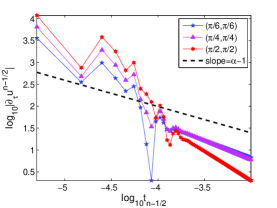
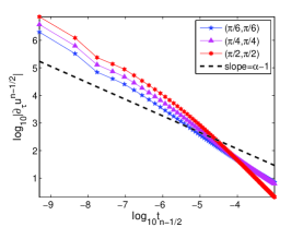
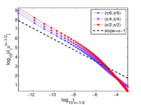
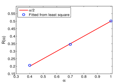
As an essential mathematical feature of linear and nonlinear subdiffusion problems including the time-fractional MBE model (1.3), the solution always lacks the smoothness near the initial time although it would be smooth away from , see [14, 15]. Actually, in any numerical methods for solving time-fractional diffusion equations, a key consideration is the initial singularity of solution, see the recent works [16, 17, 18]. More directly, we apply a new L1-type formula to the time-fractional problem (1.3), see more details in subsection 3.1 and Example 4.3. Figure 1 plots the discrete time derivative near on the graded mesh when . They suggest that
It says that the solution possesses weakly singularity like near the initial time, which can be alleviated by using the graded meshes. Thus, the second interest of this paper is to resolve the essentially weak singularity in the equation (1.3) by refining time mesh. Actually, we will show that the graded mesh can recover the optimal time accuracy when the solution is non-smooth near .
In the next section, we reformulate the time-fractional MBE model (1.3) by using SAV technique, which provides an elegant platform for constructing energy stable schemes. Although the L1 formula was applied in [13] to handle the time-fractional phase filed models and the discrete energy decay laws were also established on uniform time mesh, we are not able to exploit any discrete energy dissipation laws under the adaptive time-steps and leave it as an open problem (see Remark 1). In section 3, this open problem guides us to develop a novel numerical Caputo derivative (3.7), called L1+ formula, which preserves inherently the positive semi-definite property of integral kernel, see (3.9). This new formula is as simple as the classical L1 formula because it is also constructed by the piecewise linear interpolation; however it can achieve second-order accurate for all fractional orders and substantially improves the accuracy of L1 formula, especially when the fractional order . Applying the new formula to the time-fractional MBE model (1.3), we obtain two Crank-Nicolson SAV schemes (3.12)-(3.13) and (3.17)-(3.18), respectively. Thus it is straightforward to confirm that both of them preserve the discrete energy dissipation law well, see Theorems 3.1-3.2, so that they are unconditionally stable in the energy norm. At last, we also apply the sum-of-exponentials (SOE) technique to develop a fast L1+ algorithm in section 4. By using an accuracy criterion based adaptive time-stepping strategy, extensive numerical experiments are curried out to show the effectiveness of our numerical approaches and to support our analysis.
In summary, the main contributions of this paper for the time-fractional MBE model (1.3) are the following: suggest a simple L1+ formula of Caputo derivative having second-order accuracy for any fractional order ; apply it to build two Crank-Nicolson SAV schemes preserving the discrete energy dissipation law; and develop a fast L1+ algorithm incorporating adaptive time steps to speed up the long-time, multi-scale simulations.
2 Equivalent PDE systems
Let is a positive constant and is a nonlinear, smooth function of its argument . The Ehrlich-Schwoebel energy is given by
| (2.1) |
There are two popular choices of the nonlinear bulk potential: the double well potential, , for the case of slope selection model; and the logarithmic potential, , for the case without slope selection model. Correspondingly, the governing equation of (1.3) for the height function reads:
| (2.2) |
in which the case of slope selection model
| (2.3) |
while the case without slope selection model
| (2.4) |
In what follows, we denote the time fractional MBE model (2.2) with and without slope selection by “the Slope-Model” and “the No-Slope-Model”, respectively, for simplicity. Additionally, boundary conditions are set to be periodic so as not to complicate the analysis with unwanted details. We then reformulate the MBE models into the equivalent PDE systems by borrowing the ideas from the IEQ and SAV methods [6, 8, 7].
2.1 The Slope-Model and its equivalent system
We introduce a scalar auxiliary function in term of original variable given by
| (2.5) |
where is constant that ensures the radicand positive. Compared with those in [6, 7], the scalar auxiliary variable adds an artificial parameter to regularize the numerical approach. As a consequence, the free energy of the Slope-Model is transformed into a quadratic form
| (2.6) |
Correspondingly, the Slope-Model can be reformulated to the following equivalent form
| (2.7) | ||||
| (2.8) |
where the expression of notation given by
| (2.9) |
We should note in passing that the new system is subjected to the initial conditions
| (2.10) |
and the boundary conditions are same as the primitive model. By taking the inner product of (2.7) with , of (2.8) with , and then making time integrations on both sides, we see the equivalent system preserves the energy dissipation law
The non-positive of the right part of above equality is determined by [13, Lemma 2.1].
2.2 The No-Slope-Model and its equivalent system
For the No-Slope-Model, we introduce a scalar auxiliary function in term of original variable as follows
| (2.11) |
where and are similar to the previous ones. Therefore, the free energy of the No-Slope-Model could be rewritten into
| (2.12) |
We then could rewrite the No-Slope-Model as an equivalent form
| (2.13) | ||||
| (2.14) |
in which
| (2.15) |
with the following initial conditions
| (2.16) |
Similarly, the new system admits the following energy dissipation law
3 Novel L1+ formula and Crank-Nicolson SAV schemes
The well-known L1 formula of Caputo derivative is given by
| (3.1) |
where the corresponding discrete convolution kernels are defined by
| (3.2) |
Obviously, the discrete L1 kernels are positive and decreasing, see also [16, 17],
| (3.3) |
Based on the above L1 formula on uniform time mesh, a linearized scheme by using the stabilized technique via a stabilized term for a properly large scalar parameter is presented. We refer to [13] for more details. The resulting stabilized semi-implicit scheme for the problem (2.2) reads
| (3.4) |
It is to mention that, when the time mesh is uniform such that the discrete L1 kernels
the semi-implicit scheme (3.4) inherits a discrete energy dissipation law, see more details in [13, Theorem 3.3]. As seen, the proof of discrete version of energy dissipation law (1.6) relies on the positive semi-definite property of a discrete quadratic form .
Remark 1
It seems rather difficult to extend the positive semi-definite property to a general class of nonuniform meshes. More precisely, we are not able to verify the positive semi-definite property of the following quadratic form (by taking )
| (3.5) |
The open problem in Remark 1 motivates us to design a novel discrete Caputo formula such that it naturally possesses the energy decay law (1.6) in the discrete sense for the time-fractional MBE model. Alternatively, the novel discrete Caputo formula should inherit the positive semi-definite property of a quadratic form like (3.5).
Fortunately, as pointed out early in [19, 20], we know that the weakly singular kernel is positive semi-definite, that is,
| (3.6) |
for and any . Actually, one has for any integer and for any , then the Plancherel’s theorem implies the positive semi-definite property (3). We will see that a discrete counterpart of (3) yields a discrete Caputo approximation preserving the desired energy dissipation property (1.6) when it is applied to time-fractional MBE model (2.2).
3.1 The L1+ formula
The L1+ formula for the Caputo derivative (1.4) is defined at time as follows
| (3.7) |
where the discrete convolution kernels are defined by
| (3.8) |
Obviously, the naturally nonuniform L1+ approximation ensures the positive semi-definite property (3) by taking , that is,
| (3.9) |
The definition (3.8) and the arbitrariness of function yield the following result.
Lemma 3.1
The discrete convolution kernels in (3.8) are positive, and for any real sequence with entries, it holds that
Order Order Order 64 3.44e-05 – 3.39e-05 – 2.25e-05 – 128 8.61e-06 2.00 8.51e-06 1.99 5.83e-06 1.95 256 2.15e-06 2.00 2.13e-06 1.99 1.51e-06 1.95 512 5.38e-07 2.00 5.35e-07 2.00 3.88e-07 1.96
Before applying the L1+ formula (3.7) to the time-fractional MBE model (2.2), we show that it is a second-order approximation for the Caputo derivative (1.4) numerically. Consider a simple fractional ODE problem for , we run a Crank-Nicolson-type scheme with uniform time-steps , by choosing a smooth solution with the regularity parameter . The discrete norm errors are listed in Table 1. It seems that the numerical accuracy of (3.7) is second-order accurate for any fractional order . If the solution has an initial singularity, the L1+ formula (3.7) can also achieve the second-order accuracy by properly refining the mesh near , see more tests in Example 4.1.
3.2 Crank-Nicolson SAV schemes preserving energy dissipation
In what follows, we concern only with the time discretization of the equivalent systems, while the spatial approximation can be diverse, examples as finite difference, finite element or spectral methods. Integrating the equations (2.7)-(2.8) from to , respectively, leads to
| (3.10) | ||||
| (3.11) |
Applying the L1+ formula (3.7), the trapezoidal formula, we have the following Crank-Nicolson SAV (CN-SAV) time-stepping scheme for the Slope-Model
| (3.12) | ||||
| (3.13) |
where is the local extrapolation.
Note that, the construction of L1+ formula (3.7) implies that the above CN-SAV scheme (3.12)-(3.13) is naturally suitable for a general class of nonuniform meshes. Moreover, next result shows that it is unconditionally energy stable.
Theorem 3.1
Proof Taking the inner product of (3.12)-(3.13) with and , respectively, and adding the resulting two identities, we obtain
| (3.15) |
which implies that
| (3.16) |
By summing the superscript from to , we apply the property (3.9) to derive that
It completes the proof.
3.3 Further notes on L1+ formula
Remark 2 (Multi-term and distributed time-fractional problems)
As seen in Table 1 and more tests for Example presented in next section, the accuracy of the L1+ formula (3.7) is dependent on the regularity of solution, but would be independent of the fractional order . It is quite different from some exiting numerical approaches, such as L1, Alikhanov [21, 22] and BDF2-like formulas [23, 24, 25], of which the consistency errors are dependent on the fractional order . This feature is attractive for further applications in developing second-order approximations for multi-term and distributed-order fractional diffusion equations. For an example, consider a simple multi-term fractional diffusion problem,
where for , and is the corresponding weights. One can construct the following second-order Crank-Nicolson-type time-stepping scheme
Obviously, the L1+ formula (3.7) would be also useful in approximating the distributed-order Caputo derivative since it can be approximated by certain multi-term derivative via some proper quadrature rule, see [25].
The suggested L1+ formula (3.7) seems very promising in further applications for other time-fractional field phase models and other time-fractional differential equations. They make the rigorous theoretical analysis on consistency, stability and convergence very important, especially on a general class of nonuniform meshes.
However, the established theory [16, 26, 17, 18] for nonuniform L1 and L1-2σ (Alikhanov) formulas can not be applied to the L1+ formula directly because the corresponding discrete convolution kernels in (3.8) do not have the uniform monotonicity like (3.2). Actually, the definition (3.8) and the integral mean-value theorem yield the following result.
Lemma 3.2
The positive discrete kernels in (3.8) fulfill
Notwithstanding, it ought to be emphasized that
It is easily seen that as and as . So the value of may change the sign when the fractional order varies over . At the same time, this situation is no worse than the case in the BDF2-like formulas [24, 25] in which the second kernel would be negative when , see more details and a potential remedy technique in [26, Remark 6]. The theoretical investigations, including the consistency, stability and convergence, of nonuniform L1+ formula (3.7) will be addressed in a separate technical report.
4 Numerical algorithms and examples
4.1 A fast version of L1+ formula
It is evident that the approximations (3.1) or (3.7) are prohibitively expensive for long time simulations due to the long-time memory. Therefore, to reduce the computational cost and storage requirements, we apply the sum-of-exponentials (SOE) technique to speed up the evaluation of the L1+ formula. A core result is to approximate the kernel function efficiently on the interval , see [27, Theorem 2.5].
Lemma 4.1
For the given , an absolute tolerance error , a cut-off time and a finial time , there exists a positive integer , positive quadrature nodes and corresponding positive weights such that
The Caputo derivative (1.4) is split into the sum of a history part (an integral over ) and a local part (an integral over ) at the time , see also [17]. Then, the local part will be approximated by linear interpolation directly, the history part can be evaluated via the SOE technique, that is,
| (4.1) |
where
By utilizing the linear interpolation and a recursive formula, we can approximate by
| (4.2) |
where the positive coefficients
Having taken this excursion through (4.1)-(4.1), we arrive at the fast L1+ formula
| (4.3) |
in which is computed by using the recursive relationship
| (4.4) |
4.2 Adaptive time-stepping strategy
In the previous sections, we have proved that the numerical schemes are unconditionally energy stable which implies large time steps are allowed. Indeed, in simulating the phase field problems such as the coarsening dynamics problems discussed in Example 4.4, adaptive time-stepping strategy is necessary to efficiently resolve widely varying time scales and to significantly reduce the computational cost. Roughly speaking, the adaptive time steps can be selected by using an accuracy criterion example as [28], or the time evolution of the total energy such as [29]. We focus on the former and update the time step size by using the formula
where is a default safety coefficient, is a reference tolerance, and is the relative error at each time level. The details of the adaptive time steps strategy are presented in Algorithm 1. Here, the first-order SAV and second-order SAV schemes refer to the backward Euler-L1 method and Crank-Nicolson SAV method proposed in this article, respectively.
4.3 Numerical examples
The CN-SAV methods (3.12)-(3.13) and (3.17)-(3.18) are examined in this section for the time-fractional MBE model (2.2). Specially, the model fractional ODE problem is used in Example 4.1 to test the accuracy of L1+ formula (3.7). The time interval is always divided into two parts and with total subintervals. We will take , and apply the graded grid in to resolve the initial singularity. In the remainder interval , we put cells with random time-steps
where are the random numbers.
The time accuracy of the proposed methods is mainly focused on, so for simplicity, and the Fourier pseudo-spectral method is always applied to approximate the space variables using the same spacing in each spatial direction. To examine the CN-SAV schemes, the maximum norm error is recorded in each run, and the experimental convergence order in time is computed by
where denotes the maximum time-step size for total subintervals
Example 4.1
Consider the model fractional ODE problem with an exact solution , where the parameter determines the initial regularity of . The accuracy of L1+ formula (3.7) is examined carefully using the following three scenarios:
Order Order Order 64 2.24e-02 5.90e-03 4.65e-03 1.10e-03 128 1.16e-02 3.39e-03 0.84 2.67e-03 0.84 6.29e-04 0.84 256 5.87e-03 1.95e-03 0.82 1.53e-03 0.82 3.61e-04 0.82 512 2.88e-03 1.12e-03 0.78 8.80e-04 0.78 2.07e-04 0.78
Order Order Order 64 2.78e-02 6.47e-03 2.68e-02 1.21e-03 2.62e-02 1.68e-03 128 1.53e-02 3.23e-03 1.15 1.38e-02 3.70e-04 1.77 1.30e-02 5.04e-04 1.71 256 7.37e-03 1.63e-03 0.94 6.57e-03 8.15e-05 2.04 6.76e-03 1.55e-04 1.81 512 3.64e-03 8.20e-04 0.97 3.51e-03 2.46e-05 1.91 3.27e-03 3.77e-05 1.95
Order Order Order 64 2.76e-02 8.40e-04 2.68e-02 3.46e-04 2.71e-02 6.66e-04 128 1.49e-02 4.20e-04 1.12 1.37e-02 9.47e-05 1.93 1.30e-02 1.80e-04 1.78 256 7.34e-03 2.12e-04 0.97 6.90e-03 2.47e-05 1.95 6.76e-03 4.91e-05 1.98 512 3.65e-03 1.07e-04 0.99 3.47e-03 6.44e-06 1.96 3.26e-03 1.19e-05 1.94
Table 1 lists the case (a) having smooth solution, while Tables 2-4 record the two cases (b)-(c) having non-smooth solutions. From these numerical results in Tables 1-4, one sees that it is accurate of via the following observations: (i) The numerical accuracy is independent of the fractional order , and it is second-order accurate for smooth solutions with ; (ii) On the uniform mesh, the numerical accuracy degenerates to when the regularity parameter ; (iii) When the solution is non-smooth, the numerical accuracy reaches by the graded mesh, and the second-order accuracy would be recovered by choosing .
Example 4.2
To examine the temporal accuracy of our CN-SAV schemes, consider the time-fractional MBE model for and such that it has an exact solution .
Order Order Order 64 3.68e-02 1.78e-03 3.92e-02 5.05e-04 4.04e-02 4.63e-04 128 1.76e-02 7.87e-04 1.11 2.10e-02 1.33e-04 2.13 2.25e-02 1.19e-04 2.33 256 9.75e-03 3.43e-04 1.40 1.07e-02 3.46e-05 2.00 1.07e-02 2.96e-05 1.86 512 4.82e-03 1.49e-04 1.18 5.17e-03 8.80e-06 1.89 5.33e-03 7.39e-06 2.00
Order Order Order 64 3.96e-02 1.78e-03 4.38e-02 5.04e-04 4.26e-02 4.63e-04 128 2.02e-02 7.87e-04 1.21 2.16e-02 1.33e-04 1.88 2.23e-02 1.17e-04 2.14 256 9.74e-03 3.43e-04 1.14 1.06e-02 3.46e-05 1.89 1.07e-02 2.87e-05 1.90 512 4.96e-03 1.49e-04 1.23 5.37e-03 8.80e-06 2.02 5.51e-03 7.52e-06 2.03
The parameters are taken as , and the space is discretized by meshes. We run the CN-SAV schemes (3.12)-(3.13) and (3.17)-(3.18) by setting a variety of regularity parameters. Numerical results are tabulated in Tables 5-6, respectively. Tables 5 and 6 show the numerical results in the worse case of . It seen that it is accurate of order on the graded mesh, and the second-order accuracy can be recovered by taking . The computational results suggest that it is convergent of in time although no theoretical proof is available up to now.
Example 4.3
In what follows, if not explicitly specified, the default values of parameters are given as , and the space is discretized by meshes. To quantify the deviation of the height function, define the roughness function :
| (4.6) |
where is the average. The function characterizes the mean size of the network cell.

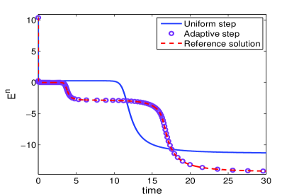
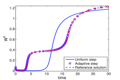
For a fixed fractional index and final time , we first apply a constant time step , i.e., , to compute the solution. Recall that the intrinsically initial singularity of solution that presented in Figure 1 early, the numerical results suggest the time mesh should be refined near the initial time. As a consequence, we could obtain the reference solution where the parameter values are applied in the cell and the uniform mesh is used over the remainder with the total numbers as before. For the adaptive time-stepping technique, taking the analogous numerical strategy in the initial time and choosing parameter and for the remainder.
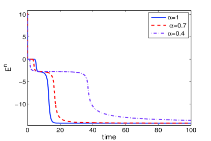
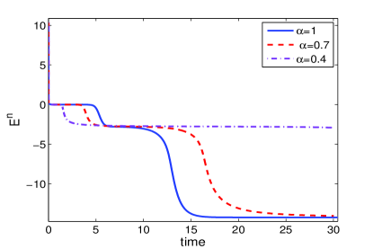
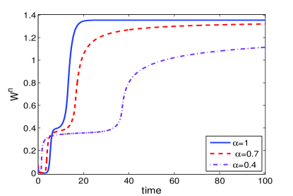
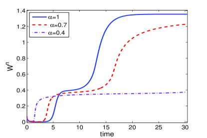
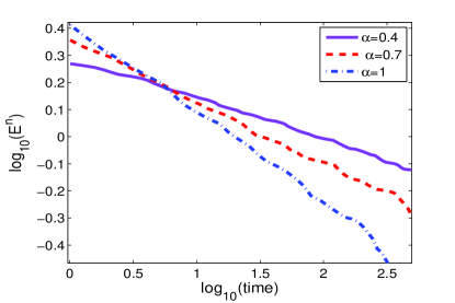
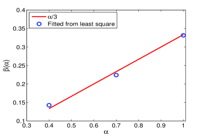
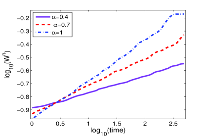
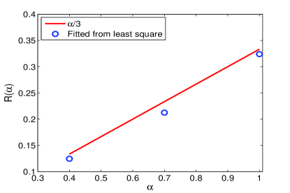
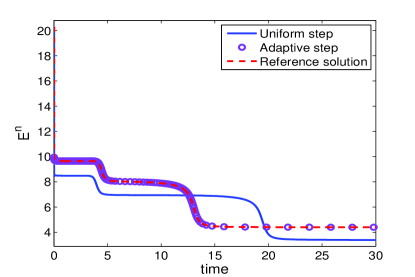
Figure 2 shows the plots of the energies and roughnesses for the Slope-Model and No-Slope-Model using uniform, graded and adaptive time steps, respectively. In our computation, we see that using uniform time step may produce incorrect steady-state solution while the energies still decay monotonically and the roughnesses show analogous plots compared with the reference solution. However, a comparison between the numerical results of using graded and adaptive time steps, we see that the curves are indistinguishable. For the adaptive strategy, the density of circle indicates the size of the time step, we then also observe that small time steps are used at the early stage of the computation because the quick transition of solution. Subsequent, large time steps are allowed due to the solution changes slowly. Again, small time steps are employed when capturing the steep structural transition from one stage to the next one. As a result, the total numbers of adaptive time steps are 4443 and 3586 for the Slope-Model and No-Slope-Model, respectively, while it takes 30000 constant time steps. The above observations show that the effect of the adaptive time approach on efficiency is significant dramatic.
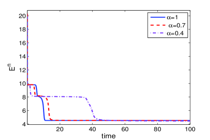
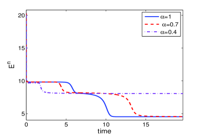
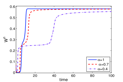
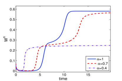
Below we make a comparison among different fractional orders to exploit how fractional index affects the evolution dynamics. Always, the third time mesh strategy is employed to solve the problem (2.2) with initial condition (4.5) in what follows. Figures 3 and 4 are the plots of the energies and roughnesses of the Slope-Model and No-Slope-Model for three different values of . We observe that in all cases the original energy decays rapidly and the smaller fractional order the faster the energy dissipates, later it decays slower as smaller fractional index , and they reach the analogous steady-state in the end. The above observations may indicate that the time-fractional operator could affects the time scaling of the evolution dynamics, while the steady-state may not be affected.
Example 4.4
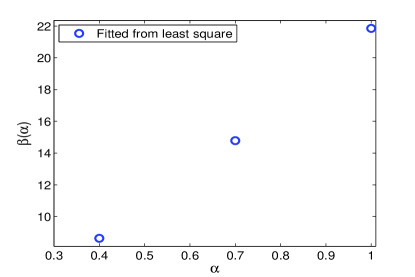
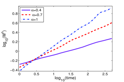
To discover the scaling of effective free energy and roughness in the time-fractional MBE model during coarsening, define the absolute value of the Slope-Model for each linear line of energy and roughness, , as
| (4.7) |
and for the No-Slope-Model, where and correspond to the energy and roughness with the fractional index , respectively.
Figures 5 and 6 show the time evolutions of energy and roughness with different fractional orders for the Slope-Model during where the adaptive time-stepping parameters and . We observe that the energy dissipation approximately as and the growth rate of the roughness is approximately as which are consistent with consistent with and , respectively, as recorded in [6, 7] for the integer Slope-Model. The time evolutions of energy and roughness for the No-Slope-Model using adaptive parameters and that are depicted in Figures 7 and 8, respectively. We see that the energy dissipation approximately as and the growth rate of the roughness is approximately as that are consistent with consistent with and as reported in [6, 7] for the integer No-Slope-Model, respectively.
Furthermore, the drawings of the Figure LABEL:Slope-Dynamics-alpha-04-07-10 displays the numerical solutions of the height function and its Laplacian for the Slope-Model with different fractional orders . Based on Figure LABEL:Slope-Dynamics-alpha-04-07-10 and additional results not shown here for brevity, we observe that the edges of the pyramids generate a random distributed network over the domain and the pyramids become large when time increases. Additionally, coarsening dynamics, at beginning, appear to be faster as smaller while it would be much slower as time evolves. Also, the observed phenomena are in good agreement with the published results [12].

5 Concluding remarks
In simulating the time-fractional phase field equations including the Molecular Beam Epitaxial model considered in this paper, the initial singularity should be treated properly because it always destroys the time accuracy of numerical algorithms especially near the initial time.
However, it seems challenging to build time-stepping approaches maintaining the discrete energy dissipation law based on the conventional L1 formula, especially on general nonuniform time meshes. Nonetheless, the energy stable schemes permitting adaptive time-stepping strategies are very attractive because they could be applicable for time-fractional phase-field models and for long-time simulations approaching the steady state. As an interesting remedy, the novel L1+ formula, is proposed to approximate the fractional Caputo’s derivative. As a consequence, coupled with the scalar auxiliary variable, we suggest two linearized second-order energy stable CN-SAV schemes for the MBE model with and without slope selection, respectively, by virtue of the naturally positive semi-definite property of a discrete quadratic form. Furthermore, for the long-time simulations approaching the steady state, the fast L1+ version incorporated with adaptive time-stepping strategy is developed for time-fractional phase field equations. Ample numerical examples are presented to validate the effectiveness of CN-SAV schemes.
The L1+ formula would be superior to some widespread approximations, such as the L1, Alikhanov and BDF2-like formulas, because it is second-order accurate for both smooth and non-smooth solutions, and the convergence order is independent of the fractional order . Thus it becomes critical to establish the rigorous theory on consistency, stability and convergence of nonuniform L1+ formula. These issues will be addressed in a forthcoming report.
References
- [1] S. Clarke and D. Vvedensky. Origin of reflection high-energy electron-diffraction intensity oscillations during molecular-beam epitaxy: a computational modeling approach. Phys. Rev. Lett., 58:2235–2238, 1987.
- [2] J. Villain. Continuum models of crystal growth from atomic beams with and without desorption. Journal De Physique I, 1:19–42, 1991.
- [3] M. Gyure, C. Ratsch, B. Merriman, R. Caflisch, S. Osher, J Zinck, and D. Vvedensky. Level-set methods for the simulation of epitaxial phenomena. Phys. Rev. E, 58:6927–6930, 1998.
- [4] J. Shen, C. Wang, X. Wang, and S. Wise. Second-order convex splitting schemes for gradient flows with ehrlich-schwoebel type energy: application to thin film epitaxy. SIAM J. Numer. Anal., 50:105–125, 2012.
- [5] C. Xu and T. Tang. Stability analysis of large time-stepping methods for epitaxial growth models. SIAM J. Numer. Anal., 44:1759–1779, 2006.
- [6] X. Yang, J. Zhao, and Q. Wang. Numerical approximations for the molecular beam epitaxial growth model based on the invariant energy quadratization method. J. Comput. Phys., 333:104–127, 2017.
- [7] Q. Cheng, J. Shen, and X. Yang. Highly efficient and accurate numerical schemes for the epitaxial thin film growth models by using the SAV approach. J. Sci. Comput., 78:1467–1487, 2019.
- [8] Y. Gong and J. Zhao. Energy-stable Runge-Kutta schemes for gradient flow models uing the energy quadratization approach. Appl. Math. Lett., 94:224–231, 2019.
- [9] Z. Li, H. Wang, and D. Yang. A space-time fractional phase-field model with tunable sharpness and decay behavior and its efficient numerical simulation. J. Comput. Phys., 347:20–38, 2017.
- [10] T. Hou, T. Tang, and J. Yang. Numerical analysis of fully discretized Crank-Nicolson scheme for fractional-in-space Allen-Cahn equations. J. Sci. Comput., 72:1–18, 2017.
- [11] H. Liu, A. Cheng, H. Wang, and J. Zhao. Time-fractional Allen-Cahn and Cahn-Hilliard phase-field models and their numerical investigation. Comp. Math. Appl., 76:1876–1892, 2018.
- [12] J. Zhao, L. Chen, and H. Wang. On power law scaling dynamics for time-fractional phase field models during coarsening. Commu. Non. Sci. Numer. Simul., 70:257–270, 2019.
- [13] T. Tang, H. Yu, and T. Zhou. On energy dissipation theory and numerical stability for time-fractional phase field equations. arXiv:1808.01471v1, 2018.
- [14] B. Jin, R. Lazarov, and Z. Zhou. An analysis of the L1 scheme for the subdiffusion equation with nonsmooth data. IMA J. Numer. Anal., 36:197–221, 2016.
- [15] B. Jin, B. Li, and Z. Zhou. Numerical analysis of nonlinear subdiffusion equations. SIAM J. Numer. Anal., 56:1–23, 2018.
- [16] H.-L. Liao, D. Li, and J. Zhang. Sharp error estimate of nonuniform L1 formula for time-fractional reaction-subdiffusion equations. SIAM J. Numer. Anal., 56:1112–1133, 2016.
- [17] H.-L. Liao, Y. Yan, and J. Zhang. Unconditional convergence of a fast two-level linearized algorithm for semilinear subdiffusion equations. J. Sci. Comput., 80(1) (2019), 1-25.
- [18] H.-L. Liao, W. Mclean, and J.Zhang. A second-order scheme with nonuniform time steps for a linear reaction-sudiffusion problem. arXiv:1803.09873v4, 2019.
- [19] W. Mclean, V. Thomée, and L. Wahlbin. Discretization with variable time steps of an evolution equation with a positive-type memory term. J. Comp. Appl. Math., 69:49–69, 1996.
- [20] W. McLean and K. Mustapha. A second-order accurate numerical method for a fractional wave equation. Numer. Math., 105:481–510, 2007.
- [21] A. Alikhanov. A new difference scheme for the time fractional diffusion equation. J. Comput. Phys., 280:424–438, 2015.
- [22] H.-L. Liao, Y. Zhao, and X. Teng. A weighted ADI scheme for subdiffusion equations. J. Sci. Comput., 69:1144–1164, 2016.
- [23] G. Gao, Z. Sun, and H. Zhang. A new fractional numerical differentiation formula to approximate the Caputo fractional derivative and its applications. J. Comput. Phys., 259:33–50, 2014.
- [24] C. Lv and C. Xu. Error analysis of a high order method for time-fractional diffusion equations. SIAM J. Sci. Comput., 38:A2699–A2724, 2016.
- [25] H.-L. Liao, P. Lyu, S. Vong, and Y. Zhao. Stability of fully discrete schemes with interpolation-type fractional formulas for distributed-order subdiffusion equations. Numer. Algo., 75:845–878, 2017.
- [26] H.-L. Liao, W. Mclean, and J. Zhang. A discrete Grönwall inequality with applications to numerical schemes for subdiffusion problems. SIAM J. Numer. Anal., 57:218–237, 2019.
- [27] S. Jiang, J. Zhang, Z. Qian, and Z. Zhang. Fast evaluation of the Caputo fractional derivative and its applications to fractional diffusion equations. Commu. Comput. Phys., 21:650–678, 2017.
- [28] H. Gomez and T. J. Hughes. Provably unconditionally stable, second-order time-accurate, mixed variational methods for phase-field models. J. Comput. Phys., 230:5310–5327, 2011.
- [29] Z. Qiao, Z. Zheng, and T. Tang. An adaptive time-stepping strategy for the molecular beam epitaxy models. SIAM J. Sci. Comput., 22:1395–1414, 2011.