Comments on the linear modified Poisson-Boltzmann equation in electrolyte solution theory

Abstract

Three analytic results are proposed for a linear form of the modified Poisson-Boltzmann equation in the theory of bulk electrolytes. Comparison is also made with the mean spherical approximation results. The linear theories predict a transition of the mean electrostatic potential from a Debye-Hückel type damped exponential to a damped oscillatory behaviour as the electrolyte concentration increases beyond a critical value. The screening length decreases with increasing concentration when the mean electrostatic potential is damped oscillatory. A comparison is made with one set of recent experimental screening results for aqueous NaCl electrolytes.

Key words: concentrated electrolytes, restricted primitive model, screening length, linear modified Poisson-Boltzmann theory

PACS: 82.45.Fk, 61.20.Qg, 82.45.Gj

Abstract

Запропоновано три аналiтичнi результати для лiнiйної форми модифiкованого рiвняння Пуассона-Больцмана в теорiї об’ємних електролiтiв. Цi результати порiвнюються з результатами середньо сферичного наближення. Лiнiйнi теорiї передбачають перехiд середнього електростатичного потенцiалу вiд загасаючої експоненцiйної поведiнки типу Дебея-Гюккеля до загасаючої осциляцiйної поведiнки при збiльшеннi концентрацiї електролiту вище критичної величини. Радiус екранування зменшується зi збiльшенням концентрацiї, коли середнiй електростатичний потенцiал загасає осциляцiйно. Проведено порiвняння з одним набором нещодавнiх експериментальних результатiв по екрануванню для водних електролiтiв NaCl.

Ключовi слова: концентрованi електролiти, обмежена примiтивна модель, радiус екранування, лiнiйна модифiкована теорiя Пуассона-Больцмана

1 Introduction

Little attention has been paid to the linear modified Poisson-Boltzmann (MPB) equation in the electrolyte solution theory, mainly due to the ready availability of the mean spherical approximation (MSA) analytical results [1]. By contrast, the non-linear MPB approach along with the hypernetted chain (HNC) [2] theory have proved two of the more successful theories in predicting the structure and thermodynamic properties of the primitive model (PM) (arbitrary sized charged hard spheres moving in a continuum dielectric) electrolyte solution [3, 4, 5]. It can be shown that the MSA is the linearized version of the HNC theory (see for example, the references [6, 7]). However, unlike the MSA, the linear MPB theory remains relatively less well explored.

In a broad sense, the usefulness of a linear theory is twofold.

Firstly, from a theoretical point of view, linear theories can and often provide valuable insights into the physics and chemistry of a situation, which might otherwise remain obscure when analyzed through their non-linear counterparts only. A case in point is the similarity (or even equivalence) between the Debye-Hückel (DH) parameter $\kappa$ [8] and the analogous MSA parameter $\Gamma=[\sqrt{(1+2\kappa a)}-1]/(2a)$ ($a$ is the ionic diameter) [1]. Although the HNC gives a more accurate solution generally, it does not lead to a physically significant quantity such as $\Gamma$. Similarly, in our case, the linear MPB (LMPB) predicts the asymptotic form of the non-linear equation and gives useful information regarding the screening length. Being based on the mean electrostatic potential approach, the linear theory is a logical extension of the Debye-Hückel (DH) theory [8]. In particular, a natural transition is given of the mean electrostatic potential behaviour in going from a DH damped exponential to a damped oscillatory as the concentration increases beyond some critical value.

Secondly, from a practical perspective, linear solutions are normally easier to obtain and are often analytic. The latter feature makes a linear solution particularly convenient to use as an initial guess in an iterative algorithm to obtain the corresponding non-linear solution.

Screening has played an important role in analysing charged systems since the electrical double layer work of Gouy and Chapman [9, 10], and that of Debye and Hückel [8] in the electrolyte bulk. The phenomenon is significant in shaping the structure and thermodynamics in these systems. A recent theoretical work on the subject is due to Rotenberg et al. [11]. The experimental screening length decreases at the higher electrolyte concentrations in contrast to that predicted by the DH theory. Smith et al. [12], Lee et al. [13] have recently investigated the experimental screening length of concentrated electrolytes. A scaling analysis [13] suggests that the decay length increases linearly with the Bjerrum length at higher concentrations. When applied to the restricted primitive model (RPM), the MSA and LMPB theories both predict a decrease in the screening length above a critical $y_{\text{c}}$ ($y=\kappa a$). Neither theory can predict the scaling result, a probable factor being the neglect of solvent effects.

In this paper we will present the mean electrostatic potential results due to three different versions of the LMPB, and compare them with the corresponding results from the MSA, the MPB, and the DH theories. The comparative behaviour of the screening properties predicted by the MPB and MSA theories will also be examined.

2 MPB theory

Improvements to the classical PB theory rest upon a more accurate pair distribution function $g_{ij}$ for two ions $i$ and $j$. In the mean electrostatic potential approach, this implies an improvement in the mean electrostatic potential $\psi(1;2)$ at the field point r₂ for an ion $i$ at r₁ through the solution of the Poisson equation

$$\nabla^{2}\psi_{i}(1;2)=-\frac{1}{\varepsilon_{0}\varepsilon_{\text{r}}}\sum_{s}e_{s}n_{s}g_{is}\,,$$ (1)

where $e_{s}$ is the charge on an ion $s$ at r₂, $n_{s}$ is the mean number density of ions of type $s$, $\varepsilon_{\text{r}}$ is the solvent relative permittivity and $\varepsilon_{0}$ is the vacuum permittivity. One technique to express the pair distribution function in terms of mean electrostatic potentials is to use Kirkwood’s charging process [14]. Taking the ion $j$ to have a charge $\lambda_{2}e_{j}$ ($0\leqslant\lambda_{2}\leqslant 1$), then the charging process gives [15, 16]

$$g_{ij}=g_{ij}(\lambda_{2}=0)\exp\left\{-\beta e_{j}\left[\psi(1;2)+\int_{0}^{1}\phi(1,2;2)\mathrm{d}\lambda_{2}\right]\right\},$$ (2)

where $\phi(1,2;3)$ is the fluctuation potential defined by

$$\psi(1,2;3)=\psi(1;3)+\psi(2;3)+\phi(1,2;3),$$ (3)

with $\psi(1,2;3)$ the mean electrostatic potential at r₃ for ions $i$ and $j$ fixed at r₁ and r₂, respectively. Thus, the fluctuation potential $\phi(1,2;3)$ describes the departure from linear superposition of the singlet potentials. Equation (2) for $g_{ij}$ is not symmetric, but a symmetric pair distribution function is obtained by charging up the ion $i$ and combining the result with equation (2) [17].

The MPB theory rests upon the closure introduced in [18]. Consider the conditional potential of mean force $W(1,2;3)$, which measures the work done in bringing an ion $s$ to r₃, given the fixed ions $i$ and $j$ at r₁ and r₂, respectively. In an analogous fashion to that for the mean electrostatic potentials, it can be written as follows:

$$W(1,2;3)=W(1,3)+W(2,3)+w(1,2,3),$$ (4)

where $w(1,2,3)$ is the corresponding departure from linear superposition of the singlet potentials of mean force. The MPB closure is

$$w(1,2,3)=e_{s}\phi(1,2;3),$$ (5)

which is analogous, but at the next hierarchical level, to the DH closure $W(1;3)=e_{s}\psi(1;3)$. Attempts to improve the DH theory by using the closure $W(1,2;3)=e_{s}\psi(1,2;3)$ fails as this closure neglects terms of the order being calculated [15, 16, 18, 19].

The governing set of differential equations for the fluctuation potential can be derived by using the Poisson equation for one or two fixed ions. This gives for the PM a two sphere potential problem which enables an approximate solution to be found for $\phi(1,2;3)$. Given an appropriate fluctuation potential, an improved pair distribution function can now be found. Previous analysis [15, 16, 17] has derived, for a RPM,

$$g_{ij}=g_{ij}^{0}\exp\left\{-\frac{\beta}{2}[e_{j}L(u_{i})+e_{i}L(u_{j})]\right\},$$ (6)

where $g_{ij}^{0}=g_{ij}(e_{i}=e_{j}=0)$,

$$L(u)=\frac{1}{2r(1+y)}\left[u(r+a)+u(r-a)+\kappa\int_{r-a}^{r+a}u(R)\mathrm{d}R\right].$$ (7)

Here, $u=r\psi(1;2)$, $r=r_{ij}$, $y=\kappa a$ with $\kappa=[\beta/(\varepsilon_{0}\varepsilon_{\text{r}})\sum_{s}e_{s}^{2}n_{s}]^{1/2}$ the DH parameter. Substituting for $g_{ij}$ in equation (1) gives the RPM non-linear MPB equation.

2.1 The linear MPB and MSA equations

The linear form of the MPB equation, for the special case of a single electrolyte with equal valences, is as follows:

$$\frac{\mathrm{d}^{2}u(r)}{\mathrm{d}r^{2}}=g_{ij}^{0}\kappa^{2}rL(u),\quad r\geqslant a,$$ (8)

with

$$u(r)=\frac{r}{a}u(a)-\frac{e_{i}(r-a)}{4\piup\varepsilon_{0}\varepsilon_{\text{r}}a}\,,\quad 0\leqslant r\leqslant a.$$ (9)

Substituting the linear solution equation (9) into equation (8) means that

$$L(u) =\frac{\kappa^{2}}{4(1+y)}\left[2u(r+a)+(r-2a)(2+2y-\kappa r)\left(\frac{\mathrm{d}u}{\mathrm{d}r}\right)_{r=a}+2(1+2y-\kappa r)u(a)+2\kappa\int_{a}^{r+a}u(R)\mathrm{d}R\right],$$

$$\hskip 284.52756pta\leqslant r\leqslant 2a.$$ (10)

Taking the Laplace transform of equation (8), with $g_{ij}^{0}=1$, gives the general solution to be of the form

$$u(r)=\sum_{n=1}^{\infty}A_{n}\exp\left(-\frac{z_{n}r}{a}\right),$$ (11)

where the sum is over the roots $z_{n}=\alpha_{n}+\mathrm{i}\beta_{n}$ of the transcendental equation

$$z\cosh(z)+y\sinh(z)=z^{3}\frac{(1+y)}{y^{2}}.$$ (12)

The roots with the smallest real part correspond to the physical situation. For small $y$, there are only two real roots with the smallest corresponding to the DH solution. As $y$ increases, the two real roots coalesce at $y_{\text{c}}=1.2412$. Above this value, the two roots move off as a complex conjugate pair until they become purely imaginary at $y_{\text{I}}=7.83$.

The MSA theory is one of the most successful and widely used theories of charged fluid systems. Although of a linear nature, its appeal lies in its analytical results, which have been applied to numerous electrolyte models and theories. The mean electrostatic potential has been studied in [20], with

$$\frac{\mathrm{d}^{2}u(r)}{\mathrm{d}r^{2}}=\kappa^{2}rL_{\text{M}}(u),\quad r\geqslant a,$$ (13)

where now

$$L_{\text{M}}=\frac{1}{2r}\left\{(1-b)^{2}[u(r+a)+u(r-a)]+\frac{2b}{a}\int_{r-a}^{r+a}\left(1-\frac{b}{a}|r-R|\right)u(R)\mathrm{d}R\right\},$$ (14)

with $b=[y+1-\sqrt{(1+2y)}]/y$. The general solution is the form of equation (11), where now $z$ satisfies the transcendental equation

$$z^{2}-2a\Gamma z+2(a\Gamma)^{2}[1-\exp{(z)}]=0,$$ (15)

with $a\Gamma=y(1-b)/2$. There are two real roots for small $y$ with the smallest corresponding to the DH solution, analogous to the MPB theory. Again, as $y$ increases, the two real roots coalesce, but at the slightly smaller value of $y_{\text{c}}=1.229$ [20, 21]. Above this critical value of $y$, the two roots become a complex conjugate pair, but unlike the MPB situation, they do not become purely imaginary for large $y$ [1]. Figure 1 displays the behaviour of the MPB and MSA roots, while a table of some of the roots is given in [15]. A critical value of $y_{\text{c}}=1.032$ was first predicted by Kirkwood [14] in his analysis of the potentials of mean force. His transcendental equation, corresponding to those of equations (12) and (15), has a behaviour pattern similar to the MPB theory. Unfortunately, his value of $y_{\text{I}}=2.79$ means that his theory is restricted to much lower concentrations than the MPB and MSA theories. Critical values of $y_{\text{c}}$ have been predicted by other theories [22, 23, 24, 25, 26].

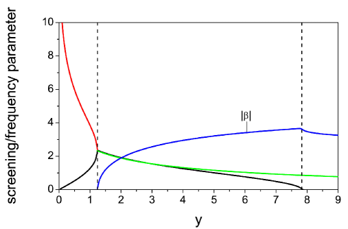
Figure 1: (Colour online) Roots of the MPB transcendental equation (12). For $y<y_{\text{c}}$ there are two real roots $\alpha_{1}$, $\alpha_{2}$ with the black (lower) curve corresponding to the DH $\kappa$ $(=\alpha_{1}/a)$ for low $y$. For $y_{\text{c}}<y<y_{\text{I}}$, the black curve represents the screening parameter $\alpha$, and the blue curve represents the screening frequency $|\beta|$. The MSA roots of equation (15) are nearly identical to those of the MPB for $y<y_{\text{c}}$, where now $y_{\text{c}}=1.229$, and are hence not shown. For $y>y_{\text{c}}$, the MSA screening parameter $\alpha$ is given by the upper green curve. The MSA does not have a finite $y_{\text{I}}$. The two vertical dashed lines at $y_{\text{c}}=1.2412$ and $y_{\text{I}}=7.831$ indicate the two MPB critical values.

We now consider $u(r)$ to be given by the two roots with the smallest real parts so that

$$u(r)=A_{1}\exp{\left(-\frac{z_{1}r}{a}\right)}+A_{2}\exp{\left(-\frac{z_{2}r}{a}\right)},\quad r\geqslant 2a,$$ (16)

with the first term corresponding to the DH value for small $y$. Both the MPB and MSA predict, above their respective $y_{\text{c}}$, that the solution is damped oscillatory [15, 16]. So, taking the complex conjugate pair $z_{1}$, $z_{2}$ to be $\alpha\pm\mathrm{i}\beta$, equation (16) can then be written as follows:

$$u(r)=A\exp{\left(-\frac{\alpha r}{a}\right)}\cos{\left(\frac{\beta r}{a}-B\right)},\quad r\geqslant 2a,$$ (17)

where $A_{1}=\bar{A}_{2}=X+\mathrm{i}Y$, $A=2\sqrt{X^{2}+Y^{2}}$, $\tan{B}=Y/X$. Equation (17) holds for the MPB when $1.2412<y<7.83$, while for the MSA when $y>1.229$. Analysis of the Ornstein-Zernike equation indicates that the asymptotic form of the correlation function takes on a similar form [27]. Equation (17) predicts, for both theories, that the screening $\alpha/a$ decreases and the frequency parameter $\beta/a$ increases for increasing $y$.

The approximate solution (16) involves two unknown constants. These cannot be determined in a unique fashion as equation (16) is simply the two leading terms of the general solution (11). A consistent analysis requires that the general solution satisfies the integro-difference differential equation in $a\leqslant r\leqslant 2a$ and the continuity of $u(a)$ and $(\mathrm{d}u/\mathrm{d}r)_{r=a}$. In this general case, the boundary conditions at $r=a$ give the neutrality condition

$$\sum_{n=1}^{\infty}A_{n}(1+z_{n})\exp{(-z_{n})}=\frac{e_{i}}{4\piup\varepsilon_{0}\varepsilon_{\text{r}}}.$$ (18)

Another general condition is that of Stillinger-Lovett [28], which is true away from the critical region of the RPM electrolyte. In terms of the mean electrostatic potential, the condition is [29]

$$\beta\sum_{s}e_{s}n_{s}\int\psi_{s}\mathrm{d}V=1.$$ (19)

Assuming that the solution (16) holds for $r\geqslant a$, then neutrality and the Stillinger-Lovett condition allows $A_{1}$ and $A_{2}$, or equivalently $A$ and $B$, to be calculated. Another approach, following Kirkwood [14], is for the solution to satisfy neutrality and equation (16) at $r=a$. A third possibility, amongst others, is to evaluate $u(r)$ in $a\leqslant r\leqslant 2a$ by substituting the solution (16) for $r\geqslant 2a$ into equation (8) and integrating twice. In this case, the boundary conditions are $u(r)$, $\mathrm{d}u(r)/\mathrm{d}r$ continuous at $r=a$ and $2a$, with neutrality and the Stillinger-Lovett condition satisfied. The three approximations are called LMPB1, LMPB2, and LMPB3, respectively. See appendix A for details. The above approximate analysis to determine the LMPB mean electrostatic potential is unnecessary for the MSA as an alternative approach gives an analytical result [20, 30]. However, this alternate formulation does not give immediately a direct identification of the MSA screening and frequency parameters.

3 Results and discussion

The physical parameters used in all the calculations were as follows: the temperature $T=298.15$ K, $a=4.25\times 10^{-10}$ m, relative permittivity $\varepsilon_{\text{r}}=78.381$ with the concentration varying from $c=0.79$ M to 18.4 M, so the range of $y$ is 1.243 to 6. Plots of the dimensionless mean electrostatic potential $\psi^{*}(r/a)$ $[=\beta|e|\psi(r/a)]$ for the 6 theories MPB, LMPB1, LMPB2, LMPB3, MSA and DH are shown in figures 2 and 3 for a uni-univalent electrolyte. Figure 2 illustrates the behaviour of $\psi^{*}$ as $y$ increases through $y_{\text{c}}$ from $y=1.243$ to $y=1.978$, and figure 3 shows the behaviour at the higher values of $y=3,4,6$. The non-linear MPB has been shown to accurately predict both the structural and thermodynamic properties of the RPM for 1:1 electrolytes, and thus is a good metric to assess the accuracy of the linear theories. For $y<y_{\text{c}}$, except for $y$ approaching $y_{\text{c}}$, all the theories are qualitatively very similar to the DH result, and hence, are not shown here. Above $y_{\text{c}}$, the theories demonstrate a damped oscillatory behaviour which cannot be predicted by the DH theory. Overall LMPB2 is in closest agreement with MPB, while surprisingly LMPB3 does relatively poorly. It would have been expected that the LMPB3 would be the most accurate because of the treatment of the region $a\leqslant r\leqslant 2a$ via equation (10). Comparison with the MPB, when the exclusion volume term is unity, brings the LMPB3 and MPB into almost quantitative agreement for $c\leqslant 18.4$ M. This indicates that the improved mean electrostatic potential treatment of the LMPB3 analysis needs to be balanced by incorporation of the uncharged hard sphere term in equation (8). An interesting feature of the LMPB3 is that besides damped oscillation terms, there is a $(r-2a)$ quadratic contribution in the region $a\leqslant r\leqslant 2a$.

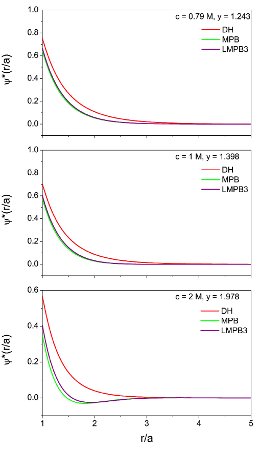
Figure 2: (Colour online) The DH, MPB and LMPB3 reduced mean electrostatic potential $\psi^{*}(r/a)$ $[=\beta|e|\psi(r/a)]$ as a function of $r/a$ for a 1:1 RPM electrolyte at $y=1.243$ ($c=0.79$ mol/dm³) (top panel), $y=1.398$ ($c=1$ mol/dm³) (middle panel), and $y=1.987$ ($c=2$ mol/dm³) (bottom panel). The LMPB1, LMPB2 and MSA results are very close to the LMPB3 result, and are not shown.

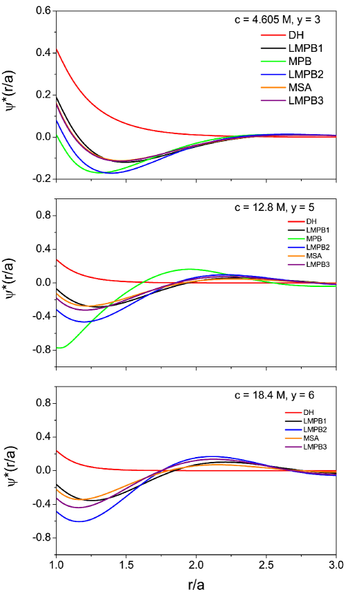
Figure 3: (Colour online) The DH, MPB, LMPB1, LMPB2, LMPB3 and MSA reduced mean electrostatic potential $\psi^{*}(r/a)$ $[=\beta|e|\psi(r/a)]$ as a function of $r/a$ for a 1:1 RPM electrolyte at $y=3$ ($c=4.605$ mol/dm${}^{3})$ (top panel), $y=5$ ($c=12.8$ mol/dm³) (middle panel), and $y=6$ ($c=18.4$ mol/dm³) (bottom panel). In the order from the lowest $\psi^{*}$(1) value, the theories are MPB, LMPB2, LMPB3, MSA, LMPB1 and DH. In the top panel, the MSA and LMPB3 overlap and in the bottom panel there is no MPB numerical solution.

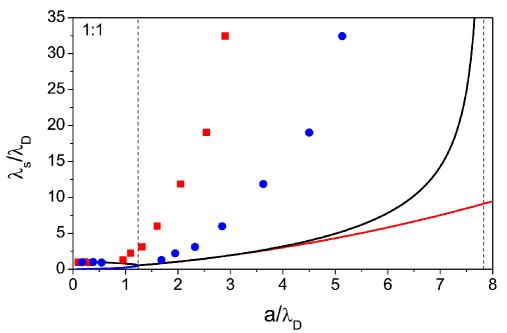
Figure 4: (Colour online) The experimental ratio $\lambda_{s}/\lambda_{\text{D}}$ for an aqueous solution of NaCl as functions of $a/\lambda_{\text{D}}$ compared with the MPB $y/\alpha_{1}$, $y/\alpha_{2}$ for $y<y_{\text{c}}$, $y/\alpha$ for $y_{\text{c}}\leqslant y\leqslant y_{\text{I}}$. The filled squares and the filled circles are the experimental results for the unhydrated ($a=2.94\times 10^{-10}$ m) and hydrated ($a=5.2\times 10^{-10}$ m) NaCl, respectively. The experimental results are taken from the Supporting Information of Smith A.M., Lee A.A., Perkin S.; electronic link given in reference [13]. The upper curve for $y<y_{\text{c}}$ is that for $\alpha_{1}$ which would be unity if it was the DH value. The MSA screening length is given by the lower red curve and is indistinguishable from the MPB value on the graphical scale for $y\leqslant 4$. The MSA does not have a finite $y_{\text{I}}$. The two vertical dashed lines at $y_{\text{c}}=1.2412$ and $y_{\text{I}}=7.831$ indicate the two MPB critical values.

Experimental results for a wide class of salts indicate that the decay length $\lambda_{s}$ of concentrated electrolytes increases with concentration, in contrast to that of the DH prediction. The LMPB and MSA also predict that their decay length $a/\alpha$, which corresponds to the experimental $\lambda_{s}$, increases at higher concentrations, but at too low a rate — see figure 4. Lee et al. [13] have analysed the electrolyte screening length behaviour at high concentration using a scaling analysis. They find that the decay length increases linearly with the Bjerrum length, or alternatively $\lambda_{s}/\lambda_{\text{D}}\sim(a/\lambda_{\text{D}})^{3}$ where $\lambda_{\text{D}}=1/\kappa$, in general agreement with experimental results for a range of 1:1 valency ionic liquids. We note that in the present paper $\lambda_{s}/\lambda_{\text{D}}=y/\alpha$ and $a/\lambda_{\text{D}}=y$ so that the experimental trend thus provides a test of theories through a study of $y/\alpha\sim y^{3}$. Unfortunately, no realistic comparisons can be made with the MPB and MSA predictions due to the decay length being too small. For example, at $y=3$, the LMPB $y/\alpha=1.95$, which is an order of magnitude too small (see figure 1 of [13]). Only for $y$ close to $y_{\text{I}}$ is the LMPB decay length of the correct order of magnitude. The most probable reason for the shortfall is the lack of any treatment of the solvent. At low to medium solution concentration, the solvent contribution can be partially treated by using an hydrated ion diameter. In figure 4, the experimental ratio $\lambda_{s}/\lambda_{\text{D}}$ for varying $a/\lambda_{\text{D}}$ is given for an aqueous solution of NaCl for $a=2.94\times 10^{-10}$ m and $a=5.2\times 10^{-10}$ m. The use of the hydrated diameter $a=5.2\times 10^{-10}$ m brings the experimental points closer to the MPB results. The high concentration of the solvent relative to the solute ions means that the structure around the ions is driven by the solvent. A step in this direction is to consider the solvent primitive model where the solvent is modelled by uncharged hard spheres moving in a constant permittivity. Recently, the underscreening in this solvent primitive model has been studied in the MSA [11]. The ratio $\lambda_{s}/\lambda_{\text{D}}$ increases at higher concentrations as required by experiment, but at too slow a rate.

4 Summary

The potential approach of the MPB theory provides a natural extension to the DH theory. At lower electrolyte concentrations, the predictions mimic the DH theory but qualitative differences occur at higher concentrations. In the region $y_{\text{c}}<y<y_{\text{I}}$, the MPB predicts a damped oscillatory potential which is in accordance with simulation and other theoretical work. For this interval of $y$, the linear potential is of the form $u(r)=A\exp{(-\alpha r/a)}\cos{(\beta r/a-B)}$, $r\geqslant 2a$, where $A$, $B$ are constants and $\alpha$, $\beta$ given by the solution of equation (12). There is no unique way of determining the constants, so three methods are considered, in each case the neutrality condition being satisfied. The Stillinger-Lovett condition is used in both the LMPB1 and LMPB3 approaches with the solution holding at $r=a$ and $r=2a$, respectively, while the LMPB2 is derived by assuming that the equation is satisfied at $r=a$. Comparison of the three theories with the accurate non-linear MPB for 1:1 salts indicates that overall the simple LMPB2 provides the best approximation. The relative poor behaviour of LMPB3 is deceptive. The LMPB3 potential is nearly identical to that of the non-linear MPB when its exclusion volume term is unity. This means that realistic improvements to the linear MPB lie through treating the exclusion volume term in the LMPB3 approach.

Experimental results have shown that the screening parameter, as interpreted via a DH type potential, initially increases as the electrolyte concentration rises, but then decreases at higher concentrations. In the LMPB theory at lower concentrations, there are two pure damped exponential terms with screening parameters $\alpha_{1}/a$, $\alpha_{2}/a$ with the smaller $\alpha_{1}/a$ corresponding to the DH screening. The parameters $\alpha_{1}$, $\alpha_{2}$ coalesce at $y_{\text{c}}$ as the concentration increases and become complex conjugate roots $\alpha\pm\mathrm{i}\beta$ for $y_{\text{c}}<y<y_{\text{I}}$. These complex conjugate roots lead to a damped oscillatory behaviour for the electrostatic potential with screening parameter $\alpha/a$. In this region of $y$, the screening parameter reduces with concentration, as seen in experiments over a similar range of $y$. The experimental results also suggest that the decay length increases linearly with the Bjerrum length. Such a behaviour is not seen in the LMPB as the rate of a decrease of the screening length is too small, only at values of $y$ close to $y_{\text{I}}$ is the screening length of the correct order of magnitude. The MSA mean electrostatic potential has features in common with the LMPB. It becomes damped oscillatory at a value of $y_{\text{c}}$ slightly less than that of the MPB, but in contrast there is no finite value of $y_{\text{I}}$. This means that its screening factor behaves in an analogous fashion to that of the MPB as $y$ increases through $y_{\text{c}}$. Above $y_{\text{c}}$, the MSA screening parameter is greater than that of the MPB and slowly reduces to zero as $y$ tends to infinity. Close agreement with experiment at the higher electrolyte concentrations is unlikely with the present PM model. A critical feature of the PM is the lack of any adequate treatment of the solvent. Models such as the solvent primitive model have provided insight as to the importance of solvent steric effects, but both the solvent and solute molecules need to be adequately modelled and treated on an equal footing.

The linear MPB equations studied here complement the full, non-linear MPB approach to the electrolyte solution theory. From a theoretical perspective, these solutions offer a valuable physical insight by painting a clearer picture of the onset of oscillations in the mean electrostatic profile and screening in electrolytes. The LMPB solutions transcend the simplistic DH view, compare favourably with the more well known MSA while retaining the simplicity and convenience of their analytic nature. Thus, the LMPB theories might well prove useful as a basis for interpreting the thermodynamic properties of concentrated electrolytes. Again, the theories could be applied to studying the liquid-gas transition in simple electrolytes in an analogous fashion to the MSA. Although the LMPB1 and LMPB3 satisfy the Stillinger-Lovett condition, this does not prohibit the LMPB1 and LMPB3 from having a solution in the liquid-gas region, as seen with the MSA. The solution of the LMPB theories is basically dependent on $y$ through the soluton of equation (12), so the theories can be solved in the simulated liquid-gas coexistence region. The pattern of the LMPB results for the range of concentration treated suggests these to be potentially very useful as initial input in the numerical solution of the full MPB equation and alternative non-linear theories.

Appendix A Analytic expressions for the three LMPB theories

A.1 $0\leqslant y\leqslant 1.2412$

Roots of equation (12), $z_{1}=\alpha_{1}$, $z_{2}=\alpha_{2}$.

$$\psi_{i}=\left[A_{1}\exp(-\alpha_{1}r/a)+A_{2}\exp(-\alpha_{2}r/a)\right]/r,\hskip 8.5359ptr\geqslant a.$$

(a) LMPB1

$$A_{1} =\frac{e_{i}}{4\piup\varepsilon_{0}\varepsilon_{\text{r}}}\exp(\alpha_{1})[\alpha_{1}^{2}G_{2}-\omega(1+\alpha_{2})]/D,$$

$$A_{2} =\frac{e_{i}}{4\piup\varepsilon_{0}\varepsilon_{\text{r}}}\exp(\alpha_{2})[-\alpha_{2}^{2}G_{1}+\omega(1+\alpha_{1})]/D,$$

$$D =\alpha_{1}^{2}(1+\alpha_{1})G_{2}-\alpha_{2}^{2}(1+\alpha_{2})G_{1}\,,\hskip 14.22636pt\omega=6\alpha_{2}^{2}/y^{2},$$

$$G_{j} =\alpha_{j}^{3}+3\alpha_{j}^{2}+6\alpha_{j}+6,\hskip 14.22636ptj=1,2.$$

(b) LMPB2, see also reference [31].

$$A_{1} =\frac{e_{i}}{4\piup\varepsilon_{0}\varepsilon_{\text{r}}}b_{2}\exp(\alpha_{1})/D,$$

$$A_{2} =-\frac{e_{i}}{4\piup\varepsilon_{0}\varepsilon_{\text{r}}}b_{1}\exp(\alpha_{2})/D,$$

$$D =b_{2}(1+\alpha_{1})-b_{1}(1+\alpha_{2}),$$

$$b_{j} =\frac{2\alpha_{j}^{2}}{\lambda}-(2+y)\alpha_{j}-2(1+y)-\frac{2y}{\alpha_{j}}-2\left(1-\frac{y}{\alpha_{j}}\right)\exp(-\alpha_{j}),\hskip 14.22636ptj=1,2,$$

$$\lambda =\frac{y^{2}}{2(1+y)}.$$

(c) LMPB3. Not given as results very detailed, see for example subsection A.2 below.

A.2 $1.2412<y<7.83$

Roots of equation (12), $z_{1}=\alpha+\mathrm{i}\beta$, $z_{2}=\alpha-\mathrm{i}\beta$.

$$\psi_{i} =(e_{i}/4\piup\varepsilon_{0}\varepsilon_{\text{r}}r)A\exp[-\alpha(r/a-1)]\cos[\beta(r/a-1)-B],\quad r\geqslant a,$$

$$A =\sqrt{X^{2}+Y^{2}}/D,\quad B=\tan^{-1}(Y/X),$$

$$R =\alpha^{2}-\beta^{2},\quad S=\alpha^{2}+\beta^{2}.$$

(a) LMPB1

$$G =G_{1}+\mathrm{i}G_{2}\,,$$

$$G_{1} =\alpha^{3}-3\alpha\beta^{2}+3\alpha^{2}-3\beta^{2}+6\alpha+6,$$

$$G_{2} =3\alpha^{2}\beta-\beta^{3}+6\alpha\beta+6\beta,$$

$$H =\frac{6}{y^{2}}S^{2},$$

$$X =\beta H-RG_{2}+2\alpha\beta G_{1}\,,$$

$$Y =(1+\alpha)H-RG_{1}+2\alpha\beta G_{2}\,,$$

$$D =(1+\alpha)X-Y\beta.$$

(b) LMPB2

From A.1 (b), $b_{1}=Y+\mathrm{i}X$, $b_{2}=Y-\mathrm{i}X$, giving

$$Y =\frac{2R}{\lambda}-(2+y)\alpha-2(1+y)-\frac{2y\alpha}{S}-2\exp(-\alpha)(p\cos\beta+q\sin\beta),$$

$$X =\frac{4\alpha\beta}{\lambda}-(2+y)\beta+2q-2\exp(-\alpha)(q\cos\beta-p\sin\beta),$$

$$D =(1+\alpha)X-Y\beta,$$

$$\lambda =\frac{y^{2}}{2(1+y)}\,,\hskip 7.11317ptp=1-\frac{y\alpha}{S}\,,\hskip 7.11317ptq=\frac{qy}{S}.$$

(c) LMPB3

$$\psi_{i} =\frac{\lambda e_{i}}{4\piup\varepsilon_{0}\varepsilon_{\text{r}}}[DX+EY+\mu(r)+c_{8}\eta(r)],\hskip 7.11317pta\leqslant r\leqslant 2a,$$

$$\psi_{i} =\frac{e_{i}}{4\piup\varepsilon_{0}\varepsilon_{\text{r}}}A\exp(-\alpha r/a)\cos{(\beta r/a-B)},\hskip 7.11317ptr\geqslant 2a,$$

$$A =2\sqrt{X^{2}+Y^{2}},\hskip 7.11317ptB=\tan^{-1}(Y/X),$$

$$\lambda =\frac{y^{2}}{2(1+y)}\,,\hskip 7.11317ptp=1-\frac{y\alpha}{S}\,,\hskip 7.11317ptq=\frac{y\beta}{S}\,,$$

$$R =\alpha^{2}-\beta^{2},\hskip 7.11317ptS=\alpha^{2}+\beta^{2},$$

$$x =\frac{r-2a}{a}\,,$$

$$c_{1} =\frac{6y^{3}}{12+12y-y^{3}}\,,$$

$$c_{2} =\frac{120y^{2}}{240+240y+y^{2}(60+15c_{1}+40y+4yc_{1})}\,,$$

$$c_{3} =\frac{5c_{1}}{24}\,,$$

$$c_{4} =\frac{1}{24}(4c_{3}+5)+\frac{y}{120}(5c_{3}+6)+d_{2}c_{8}\,,$$

$$c_{5} =1-\frac{y^{2}(3+2c_{8})}{6}-\frac{y^{4}c_{4}}{2(1+y)}\,,$$

$$c_{6} =\frac{19}{120}+\frac{29y}{720}+\frac{c_{3}}{8}+\frac{yc_{3}}{30}\,,$$

$$c_{7} =1-y^{2}\left[\frac{3}{2}+\frac{2y}{3}+\frac{c_{1}(4+y)}{16}+c_{8}c_{9}\right],$$

$$c_{8} =-c_{2}\frac{24+4c_{1}+12y+yc_{1}}{24}\,,$$

$$c_{9} =\frac{200+110y+3c_{1}(15+4y)}{240}\,,$$

$$d_{1} =p\left(1+\frac{\alpha}{S}\right)+\frac{q^{2}}{y}+\frac{3y}{2}\,,$$

$$d_{2} =\beta\frac{y(S+2\alpha)-S}{S^{2}}\,,$$

$$D =K+D_{1}+Mx+\left[\frac{c_{1}V}{2}+\frac{y\exp(-2\alpha)B_{4}}{S}\right]x^{2}+M_{3}\eta(r),$$

$$E =L+E_{1}+Nx+\left[\frac{c_{1}W}{2}+\frac{y\exp(-2\alpha)B_{5}}{S}\right]x^{2}+N_{3}\eta(r),$$

$$D_{1} =\frac{2\exp\left[-\left(\frac{r}{a}+1\right)\alpha\right](Rs_{1}+2\alpha\beta s_{2})}{S^{2}}\,,$$

$$E_{1} =\frac{2\exp\left[-\left(\frac{r}{a}+1\right)\alpha\right](2\alpha\beta s_{1}-Rs_{2})}{S^{2}}\,,$$

$$s_{1} =p\cos\left[\beta\left(\frac{r}{a}+1\right)\right]+q\sin\left[\beta\left(\frac{r}{a}+1\right)\right],$$

$$s_{2} =q\cos\left[\beta\left(\frac{r}{a}+1\right)\right]-p\sin\left[\beta\left(\frac{r}{a}+1\right)\right],$$

$$\eta(r) =\frac{1}{240}\left[c_{1}(15+4y)+120+40(1-y)x-10x^{2}\right]x^{2},$$

$$\mu(r) =\frac{1}{48}[c_{1}(4+y)+24]x^{2}-\frac{y}{6}x^{3},$$

$$K =\frac{2}{\lambda}\exp(-2\alpha)\cos 2\beta-\frac{2}{s^{2}}(RB_{2}+2\alpha\beta B_{3})\exp(-3\alpha),$$

$$L =\frac{2}{\lambda}\exp(-2\alpha)\sin 2\beta-\frac{2}{s^{2}}(2\alpha\beta B_{2}-RB_{3})\exp(-3\alpha),$$

$$B_{2} =p\cos 3\beta+q\sin 3\beta,\hskip 14.22636ptB_{22}=p\cos 2\beta+q\sin 2\beta,$$

$$B_{3} =q\cos 3\beta-p\sin 3\beta,\hskip 14.22636ptB_{32}=q\cos 2\beta-p\sin 2\beta,$$

$$B_{4} =\alpha\cos 2\beta-\beta\sin 2\beta,$$

$$B_{5} =\beta\cos 2\beta+\alpha\sin 2\beta,$$

$$B_{6} =\left(1+\frac{\alpha}{S}\right)\cos 2\beta-\frac{\beta}{S}\sin 2\beta,$$

$$B_{7} =\left(1+\frac{\alpha}{S}\right)\sin 2\beta+\frac{\beta}{S}\cos 2\beta,$$

$$B_{8} =\left(2+\frac{\alpha}{S}\right)\cos 3\beta-\frac{\beta}{S}\sin 3\beta,$$

$$B_{9} =\left(2+\frac{\alpha}{S}\right)\sin 3\beta+\frac{\beta}{S}\cos 3\beta,$$

$$\delta_{1} =\alpha^{3}-3\alpha\beta^{2},\hskip 7.11317pt\delta_{2}=\beta^{3}-3\beta\alpha^{2},$$

$$M =\frac{2}{S}(\alpha B_{2}+\beta B_{3})\exp(-3\alpha)-\frac{2}{\lambda}(\alpha\cos 2\beta+\beta\sin 2\beta)\exp(-2\alpha),$$

$$N =\frac{2}{S}(\beta B_{2}-\alpha B_{3})\exp(-3\alpha)-\frac{2}{\lambda}(\alpha\sin 2\beta-\beta\cos 2\beta)\exp(-2\alpha),$$

$$P =\left\{\frac{y}{3S}B_{4}+\frac{2}{S^{3}}\left[\delta_{1}B_{22}-\delta_{2}B_{32}-(\delta_{1}B_{2}-\delta_{2}B_{3})\exp(-\alpha)\right]\right\}\exp(-2\alpha),$$

$$Q =\left\{\frac{y}{3S}B_{5}+\frac{2}{S^{3}}\left[-\delta_{2}B_{22}-\delta_{1}B_{32}+(\delta_{2}B_{2}+\delta_{1}B_{3})\exp(-\alpha)\right]\right\}\exp(-2\alpha),$$

$$V =K-\frac{M}{2}+P,$$

$$W =L-\frac{N}{2}+Q,$$

$$V_{1} =\frac{2}{S}\exp(-2\alpha)(d_{1}B_{4}+d_{2}B_{5}),$$

$$W_{1} =\frac{2}{S}\exp(-2\alpha)(d_{1}B_{5}-d_{2}B_{4}),$$

$$M_{2} =\frac{2}{S}\left\{\beta[-q\cos 2\beta+(y+p)\sin 2\beta]-\alpha[(y+p)\cos 2\beta+q\sin 2\beta]\right\}\exp(-2\alpha),$$

$$N_{2} =\frac{2}{S}\left\{\alpha[q\cos 2\beta-(y+p)\sin 2\beta]-\beta[(y+p)\cos 2\beta+q\sin 2\beta]\right\}\exp(-2\alpha),$$

$$M_{3} =c_{2}(M-c_{1}V+M_{2}),\hskip 7.11317ptN_{3}=c_{2}(N-c_{1}W+N_{2}),$$

$$K_{2} =\Big{\{}\frac{5y}{12S}B_{4}+\frac{2}{S^{3}}\left[\delta_{1}(pB_{6}+qB_{7})-\delta_{2}(qB_{6}-pB_{7})\right]$$

$$-\exp(-\alpha)[\delta_{1}(pB_{8}+qB_{9})+\delta_{2}(pB_{9}-qB_{8})]\Big{\}}\exp(-2\alpha),$$

$$L_{2} =\Big{\{}\frac{5y}{12S}B_{5}+\frac{2}{S^{3}}\left[-\delta_{2}(pB_{6}+qB_{7})+\delta_{1}(qB_{7}-pB_{6})\right]$$

$$+\exp(-\alpha)[\delta_{2}(pB_{8}+qB_{9})-\delta_{1}(pB_{9}-qB_{8})]\Big{\}}\exp(-2\alpha),$$

$$K_{3} =\frac{3K}{2}-\frac{2M}{3}+\frac{5c_{3}V}{24}+K_{2}\,,$$

$$L_{3} =\frac{3L}{2}-\frac{2N}{3}+\frac{5c_{3}W}{24}+L_{2}\,,$$

$$M_{4} =\lambda\left(K-2M+\frac{3c_{1}V}{2}+V_{1}+c_{9}M_{3}\right),$$

$$N_{4} =\lambda\left(L-2N+\frac{3c_{1}W}{2}+W_{1}+c_{9}N_{3}\right),$$

$$F =\frac{2}{S}y^{2}\exp(-2\alpha)\left[2B_{4}+\frac{1}{s}(R\cos 2\beta-2\alpha\beta\sin 2\beta)\right],$$

$$G =\frac{2}{S}y^{2}\exp(-2\alpha)\left[2B_{5}+\frac{1}{s}(R\sin 2\beta+2\alpha\beta\cos 2\beta)\right],$$

$$F_{1} =\frac{y^{2}M_{3}}{3}+\lambda y^{2}(K_{3}+c_{6}M_{3})+F,$$

$$G_{1} =\frac{y^{2}N_{3}}{3}+\lambda y^{2}(L_{3}+c_{6}N_{3})+G,$$

$$X =\frac{N_{4}c_{5}-G_{1}c_{7}}{D_{0}}\,,$$

$$Y =\frac{F_{1}c_{7}-M_{4}c_{5}}{D_{0}}\,,$$

$$D_{0} =N_{4}F_{1}-G_{1}M_{4}.$$

Ukrainian 0

Коментарi стосовно лiнiйного модифiкованого рiвняння Пуассона-Больцмана в теорiї розчинiв електролiтiв

К.Б. Оутвайт${}^{\textsf{\footnotesize{\mbox{?}}}}$, Л.Б. Бхуян${}^{\textsf{\footnotesize{\mbox{?}}}}$

             
${}^{\textsf{\footnotesize 1}}$ Факультет прикладної математики, Унiверситет Шеффiлда, Шеффiлд, Великобританiя ${}^{\textsf{\footnotesize 2}}$ Лабораторiя теоретичної фiзики, Унiверситет Пуерто Рiко, Пуерто Рiко, США

References

• [1] Blum L., In: Theoretical Chemistry, Advances and Perspectives, Vol. 5, Eyring H., Henderson H. (Eds.), Academic Press, New York, 1980, 1.
• [2] Friedman H.L., A Course in Statistical Mechanics, Prentice Hall, New Jersey, 1985.
• [3] Vlachy V., Annu. Rev. Phys. Chem., 1999, 50, 145, doi:10.1146/annurev.physchem.50.1.145.
• [4] Bhuiyan L.B., Vlachy V., Outhwaite C.W., Int. Rev. Phys. Chem., 2002, 21, 1, doi:10.1080/01442350110078842.
• [5] Quiñones A.O., Bhuiyan L.B., Outhwaite C.W., Condens. Matter Phys., 2018, 21, 23802,
doi:10.5488/CMP.21.23802.
• [6] Henderson D., Blum L., J. Electroanal. Chem. Interfacial Electrochem., 1978, 93, 151,
doi:10.1016/S0022-0728(78)80228-9.
• [7] Henderson D., Blum L., J. Chem. Phys., 1979, 70, 3149, doi:10.1063/1.437813.
• [8] Debye P., Hückel E., Z. Phys., 1923, 24, 185.
• [9] Gouy G., J. Phys. Theor. Appl., 1910, 9, 457, doi:10.1051/jphystap:019100090045700.
• [10] Chapman D.L., Philos. Mag., 1913, 25, 475, doi:10.1080/14786440408634187.
• [11] Rotenberg B., Bernard O., Hansen J.-P., J. Phys.: Condens. Matter, 2018, 30, 054005,
doi:10.1088/1361-648X/aaa3ac.
• [12] Smith A.M., Lee A.A., Perkin S., J. Phys. Chem. Lett., 2016, 7, 2157, doi:10.1021/acs.jpclett.6b00867.
• [13] Lee A.A., Perez-Martinez C.S., Smith A.M., Perkin S., Phys. Rev. Lett., 2017, 119, 026002,
doi:10.1103/PhysRevLett.119.026002.
• [14] Kirkwood J.G., Chem. Rev., 1936, 19, 275, doi:10.1021/cr60064a007.
• [15] Outhwaite C.W., In: Statistical Mechanics, Vol. 2, Singer K. (Ed.), The Chemical Society, London, 1975, 188–255, doi:10.1039/9781847556936-00188.
• [16] Outhwaite C.W., Condens. Matter Phys., 2004, 7, 719, doi:10.5488/CMP.7.4.719.
• [17] Outhwaite C.W., Molero M., Bhuiyan L.B., J. Chem. Soc., Faraday Trans., 1991, 87, 3227,
doi:10.1039/FT9918703227.
• [18] Outhwaite C.W., J. Chem. Phys., 1969, 50, 2277, doi:10.1063/1.1671378.
• [19] Kirkwood J.G., J. Chem. Phys., 1934, 2, 767, doi:10.1063/1.1749393.
• [20] Outhwaite C.W., Hutson V.C.L., Mol. Phys., 1975, 29, 1521, doi:10.1080/00268977500101331.
• [21] Hafskjold B., Stell G., In: The Liquid State of Matter: Fluids, Simple and Complex, Montroll W.L., Lebowitz J.L. (Eds.), North-Holland Publishing Company, Amsterdam, New York, Oxford, 1982, 175.
• [22] Martynov G.A., Sov. Electrochem., 1965, 1, 285.
• [23] Martynov G.A., Sov. Electrochem., 1965, 1, 484.
• [24] Rasaiah J., Chem. Phys. Lett., 1970, 7, 260, doi:10.1016/0009-2614(70)80303-7.
• [25] Kjellander R., J. Phys. Chem., 1995, 99, 10392, doi:10.1021/j100025a048.
• [26] Lee B.P., Fisher M., Europhys. Lett., 1997, 39, 611, doi:10.1209/epl/i1997-00402-x.
• [27] Leote de Carvalho R.J.F., Evans R., Mol. Phys., 1994, 83, 619, doi:10.1080/00268979400101491.
• [28] Stillinger F.H., Lovett R., J. Chem. Phys., 1968, 48, 3858, doi:10.1063/1.1669709.
• [29] Outhwaite C.W., Chem. Phys. Lett., 1974, 24, 73, doi:10.1016/0009-2614(74)80216-2.
• [30] Henderson D., Smith W.R., J. Stat. Phys., 1978, 19, 191, doi:10.1007/BF01012511.
• [31] Outhwaite C.W., Mol. Phys., 1971, 20, 705, doi:10.1080/00268977100100671.