Approximate Causal Abstraction

Abstract

Scientific models describe natural phenomena at different levels of abstraction. Abstract descriptions can provide the basis for interventions on the system and explanation of observed phenomena at a level of granularity that is coarser than the most fundamental account of the system. Beckers and Halpern BH19, building on work of Rubenstein et al. Rub17, developed an account of abstraction for causal models that is exact. Here we extend this account to the more realistic case where an abstract causal model offers only an approximation of the underlying system. We show how the resulting account handles the discrepancy that can arise between low- and high-level causal models of the same system, and in the process provide an account of how one causal model approximates another, a topic of independent interest. Finally, we extend the account of approximate abstractions to probabilistic causal models, indicating how and where uncertainty can enter into an approximate abstraction.

1 INTRODUCTION

Scientific models aim to provide a description of reality that offers both an explanation of observed phenomena and a basis for intervening on and manipulating the system to bring about desired outcomes. Both of these aims lead to a consideration of models that represent the causal relations governing the system. They also imply the need for scientific models that describe the system at a granularity or level of description appropriate for the user and suitable for interventions that are feasible. Such more abstract causal models do not capture all the detailed interactions that occur at the most fundamental level of the system, nor do they, in general, represent outcomes of the system completely accurately at the abstract level. Nevertheless, such abstract causal models can (at least) approximately explain the phenomena, and can be informative about how the system will respond to interventions that are specified only at the abstract level.

This paper provides a formal account of such approximate abstractions for causal models that builds on the definition of an abstraction provided by Beckers and Halpern BH19 (see Section 2), which in turn built on the work of Rubenstein et al. Rub17. That notion of abstraction implicitly assumed an underlying causal system that permitted an exact description of the system at the abstract level. Here we weaken that assumption to handle what we take to be the more realistic case, namely, that abstract causal models will capture the underlying system in only an approximate way.

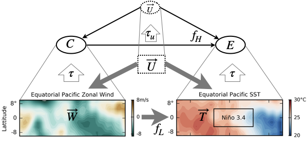
Figure 1: Climate example adapted from Chalupka et al. (2016), in which a high-level causal model for the phenomenon of El Niño is constructed from low-level (high-dimensional) wind $\vec{W}$ and sea surface temperature $\vec{T}$ measurements. $\vec{U}$ is an unmeasured confounder and $\tau$ is the mapping between the models. See text for details.

As a simplified working example to illustrate our points we use the case of the wind and sea surface temperature patterns over the equatorial Pacific that give rise to the high-level climate phenomena of El Niño and La Niña, as described by Chalupka et al. CBPE16. They considered the question of how the El Niño climate phenomenon related to the underlying wind and sea surface temperature patterns that constitute it (see Fig. 1). At the low level they considered two high-dimensional vector-valued variables representing the wind speeds $\vec{W}$ and the sea surface temperatures $\vec{T}$, respectively, on a grid of geographical locations in the equatorial Pacific. They assumed (with some justification from climate science) that wind speed $\vec{W}$ is a cause of sea surface temperature $\vec{T}$, that is, $\vec{T}=f_{L}(\vec{W},\vec{U})$ for some high-dimensional function $f_{L}(.)$ and exogenous causes $\vec{U}$. They allowed the possibility that $\vec{U}$ may be a confounder of $\vec{W}$ and $\vec{T}$, so that there might be an additional causal relation $\vec{W}=g_{L}(\vec{U})$. Leaving details about feedback and temporal delay aside, they were interested in whether the same system could be described at a higher level, using a low-dimensional structural equation $E=f_{H}(C,\vec{U})$, where there is a surjective mapping $\tau$ from ${\cal R}(\vec{T},\vec{W})$, the set of possible values of $\vec{T}$ and $\vec{W}$, to ${\cal R}(E,C)$. In the language of this paper, they were searching for an abstract causal description of the system. They required that the high-level model retain a causal interpretation, in the sense that if one intervened on $C$, there would still be a well-defined causal effect on $E$, no matter how the intervention on $C$ was interpreted as an intervention on the underlying set of variables $\vec{W}$.

Chalupka et al. CBPE16 were able to learn such a high-level model, and one of the states of $E$ (the high-level description of the sea surface temperatures) indeed corresponded to what would commonly be described as an El Niño occurring, conventionally defined by an average temperature deviation in a rectangular region of the Pacific. However, the high-level description was not perfect: it provided an informative causal description of the underlying systems and allowed for predictions that approximated the actual outcomes. Here we make precise the nature of such an approximation between a high-level and low-level causal model of the same system. In the process, we define what it means for one causal model to approximate another.

Although our running example is a vastly simplified climate model, the challenge of approximately modeling phenomena at a more abstract level is part of almost every scientific model. For example, it was Robert Boyle’s great insight that, despite its inaccuracies for real gases in practice, the ideal gas law still provides an approximate abstract description of the behavior of the molecules of a gas in a container that is extraordinarily useful for understanding and manipulating real systems. Approximate abstractions can take a variety of forms in scientific practice, ranging from idealizations and discretizations to other forms of simplification and dimension reduction (as in the climate example). Our account captures these in a unified formal framework.

The main contribution of this paper is to present a framework that offers a foundation for analyzing abstraction and approximation in causal models. We provide what we believe are sensible definitions of approximation and approximate abstraction, and a conceptual discussion of these notions. In addition, we provide some technical results regarding the difficulty of determining whether an approximate abstraction can be viewed as the composition of an approximation and an exact abstraction.

2 PRELIMINARIES

Since we are interested in scientific models that support explanations of phenomena and can inform interventions on a system, we start by defining a deterministic causal model with a set of possible interventions. We use exogenous and endogenous variables to distinguish those influences that are external to the system and those that are internal. The definitions follow the framework developed by Halpern Hal48.

Definition 2.1

: A signature ${\cal S}$ is a tuple $({\cal U},{\cal V},{\cal R})$, where ${\cal U}$ is a set of exogenous variables, ${\cal V}$ is a set of endogenous variables, and ${\cal R}$, a function that associates with every variable $Y\in{\cal U}\cup{\cal V}$ a nonempty set ${\cal R}(Y)$ of possible values for $Y$ (i.e., the set of values over which $Y$ ranges). If $\vec{X}=(X_{1},\ldots,X_{n})$, ${\cal R}(\vec{X})$ denotes the crossproduct ${\cal R}(X_{1})\times\cdots\times{\cal R}(X_{n})$.  

For simplicity in this paper, we assume that signatures are finite, that is, ${\cal U}$ and ${\cal V}$ are finite, and the range of each variable $Y\in{\cal U}\cup{\cal V}$ is finite.

Definition 2.2

: A basic causal model $M$ is a pair $({\cal S},{\cal F})$, where ${\cal S}$ is a signature and ${\cal F}$ defines a function that associates with each endogenous variable $X$ a structural equation $F_{X}$ giving the value of $X$ in terms of the values of other endogenous and exogenous variables. Formally, the equation $F_{X}$ maps ${\cal R}({\cal U}\cup{\cal V}-\{X\})$ to ${\cal R}(X)$, so $F_{X}$ determines the value of $X$, given the values of all the other variables in ${\cal U}\cup{\cal V}$.  

Note that there are no functions associated with exogenous variables, since their values are determined outside the model. We call a setting $\vec{u}$ of values of exogenous variables a context.

The value of $X$ may not depend on the values of all other variables. $Y$ depends on $X$ in context $\vec{u}$ if there is some setting of the endogenous variables other than $X$ and $Y$ such that if the exogenous variables have value $\vec{u}$, then varying the value of $X$ in that context results in a variation in the value of $Y$; that is, there is a setting $\vec{z}$ of the endogenous variables other than $X$ and $Y$ and values $x$ and $x^{\prime}$ of $X$ such that $F_{Y}(x,\vec{z},\vec{u})\neq F_{Y}(x^{\prime},\vec{z},\vec{u})$.

In this paper, we restrict attention to recursive (or acyclic) models, that is, models where there is a partial order $\preceq$ on variables such that if $Y$ depends on $X$, then $X\prec Y$. In a recursive model, given a context $\vec{u}$, the values of all the remaining variables are determined (we can just solve for the value of the endogenous variables in the order given by $\prec$) We often write the equation for an endogenous variable as $X=f(\vec{Y})$; this denotes that the value of $X$ depends only on the values of the variables in $\vec{Y}$, and the connection is given by $f$. Our climate example is recursive, since $\vec{T}=f_{L}(\vec{W},\vec{U})$.

An intervention has the form $\vec{X}\leftarrow\vec{x}$, where $\vec{X}$ is a set of endogenous variables. Intuitively, this means that the values of the variables in $\vec{X}$ are set to $\vec{x}$. The structural equations define what happens in the presence of interventions. Setting the value of some variables $\vec{X}$ to $\vec{x}$ in a causal model $M=({\cal S},{\cal F})$ results in a new causal model, denoted $M_{\vec{X}\leftarrow\vec{x}}$, which is identical to $M$, except that ${\cal F}$ is replaced by ${\cal F}^{\vec{X}\leftarrow\vec{x}}$: for each variable $Y\notin\vec{X}$, $F^{\vec{X}\leftarrow\vec{x}}_{Y}=F_{Y}$ (i.e., the equation for $Y$ is unchanged), while for each $X^{\prime}$ in $\vec{X}$, the equation $F_{X^{\prime}}$ for is replaced by $X^{\prime}=x^{\prime}$ (where $x^{\prime}$ is the value in $\vec{x}$ corresponding to $\vec{x}$).

Halpern and Pearl HP01b and Halpern Hal48 implicitly assumed that all interventions can be performed in a model. For reasons that will become clear when defining abstraction, we follow Rubenstein et al. Rub17 and Beckers and Halpern BH19 in adding the notion of “allowed interventions” to a causal model. This allows us to capture situations where not all interventions are of interest to the modeler and/or some interventions may not be feasible. We can then define a causal model $M$ as a tuple $({\cal S},{\cal F},{\cal I})$, where $({\cal S},{\cal F})$ is a basic causal model and ${\cal I}$ is a set of allowed interventions. We sometimes write a causal model $M=({\cal S},{\cal F},{\cal I})$ as $(M^{\prime},{\cal I})$, where $M^{\prime}$ is the basic causal model $({\cal S},{\cal F})$, if we want to emphasize the role of the allowed interventions.

Given a signature ${\cal S}=({\cal U},{\cal V},{\cal R})$, a primitive event is a formula of the form $X=x$, for $X\in{\cal V}$ and $x\in{\cal R}(X)$. A causal formula (over ${\cal S}$) is one of the form $[Y_{1}\leftarrow y_{1},\ldots,Y_{k}\leftarrow y_{k}]\varphi$, where $\varphi$ is a Boolean combination of primitive events, $Y_{1},\ldots,Y_{k}$ are distinct variables in ${\cal V}$, and $y_{i}\in{\cal R}(Y_{i})$. Such a formula is abbreviated as $[\vec{Y}\leftarrow\vec{y}]\varphi$. The special case where $k=0$ is abbreviated as $\varphi$. Intuitively, $[Y_{1}\leftarrow y_{1},\ldots,Y_{k}\leftarrow y_{k}]\varphi$ says that $\varphi$ would hold if $Y_{i}$ were set to $y_{i}$, for $i=1,\ldots,k$.

A causal formula $\psi$ is true or false in a causal model, given a context. As usual, we write $(M,\vec{u})\models\psi$ if the causal formula $\psi$ is true in causal model $M$ given context $\vec{u}$. The $\models$ relation is defined inductively. $(M,\vec{u})\models X=x$ if the variable $X$ has value $x$ in the unique (since we are dealing with recursive models) solution to the equations in $M$ in context $\vec{u}$ (i.e., the unique vector of values that simultaneously satisfies all equations in $M$ with the variables in ${\cal U}$ set to $\vec{u}$). The truth of conjunctions and negations is defined in the standard way. Finally, $(M,\vec{u})\models[\vec{Y}\leftarrow\vec{y}]\varphi$ if $(M_{\vec{Y}=\vec{y}},\vec{u})\models\varphi$.

To simplify notation, we sometimes write $M(\vec{u})$ to denote the unique element of ${\cal R}({\cal V})$ such that $(M,\vec{u})\models{\cal V}=\vec{v}$. Similarly, given an intervention $\vec{Y}\leftarrow\vec{y}$, $M(\vec{u},\vec{Y}\leftarrow\vec{y})$ denotes the unique element of ${\cal R}({\cal V})$ such that $(M,\vec{u})\models[\vec{Y}\leftarrow\vec{y}]({\cal V}=\vec{v})$.

These definitions allow us to describe the climate system both in terms of a low-level causal model $M_{L}$ and a high-level model $M_{H}$:

$$M_{L} =(({\cal U}_{L},{\cal V}_{L},{\cal R}_{L}),{\cal F}_{L},{\cal I}_{L})$$

$$=((\{\vec{U}\},\{\vec{W},\vec{T}\},{\cal R}_{L}),\{g_{L},f_{L}\},{\cal I}_{L})\mbox{ and }$$

$$M_{H} =(({\cal U}_{H},{\cal V}_{H},{\cal R}_{H}),{\cal F}_{H},{\cal I}_{H})$$

$$=((\{\vec{U}\},\{C,E\},{\cal R}_{H}),\{g_{H},f_{H}\},{\cal I}_{H}).$$

Chalupka et al. CBPE16 treated $\vec{U}$ as not only exogenous, but also unobserved, and therefore made no claim about its dimensionality in the high-level model. We do not explicitly spell out ${\cal R}_{L}$ and ${\cal R}_{H}$ here; the description of the climate model indicates that ${\cal R}_{L}(C)\times{\cal R}_{L}(E)$ is much smaller than ${\cal R}_{L}(\vec{W})\times{\cal R}_{L}(\vec{T})$: many different low-level (vector-valued) states may correspond to one high-level low-dimensional state. Finally, for our climate example we have not yet said anything about interventions, so ${\cal I}_{L}$ and ${\cal I}_{H}$ are currently placeholders.

We are now in a position to specify a relation between the high and low-level models $M_{H}$ and $M_{L}$.

2.1 Abstraction

Beckers and Halpern BH19 gave a sequence of successively more restrictive definitions of abstraction for causal model. The first and least restrictive definition is the notion of exact transformation due to Rubenstein et al. Rub17. Examples given by Beckers and Halpern show that the notion of exact transformation is arguably too flexible. Thus, in this paper the notion of abstraction we consider is that of $\tau$-abstractions, introduced by Beckers and Halpern, which can be viewed as a restriction of exact transformations and avoids some of their problems. However, nothing hinges on this choice: all definitions can just as well be interpreted using the less restrictive notions of abstractions.

The key to defining all the notions of abstraction from a low-level to a high-level causal model considered by Beckers and Halpern is the abstraction function $\tau:{\cal R}_{L}({\cal V}_{L})\rightarrow{\cal R}_{H}({\cal V}_{H})$ that maps endogenous states of $M_{L}$ to endogenous states of $M_{H}$. This is a generalization of the surjective mapping $\tau$ from ${\cal R}(\vec{T},\vec{W})$ to ${\cal R}(E,C)$ discussed in the introduction. In the formal definition, we need two additional functions: $\tau_{{\cal U}}:{\cal R}_{L}({\cal U}_{L})\rightarrow{\cal R}_{H}({\cal U}_{H})$, which maps exogenous states of $M_{L}$ to exogenous states of $M_{H}$, and $\omega_{\tau}:{\cal I}_{L}\rightarrow{\cal I}_{H}$, which maps low-level interventions to high-level interventions. Beckers and Halpern BH19 show that, given their definition of abstraction, $\tau_{{\cal U}}$ and $\omega_{\tau}$ can be derived from $\tau$. We briefly review the relevant definitions here; we refer the reader to their paper for more details and motivation.

Definition 2.3

: Given a set ${\cal V}$ of endogenous variables, $\vec{X}\subseteq{\cal V}$, and $\vec{x}\in{\cal R}(\vec{X})$, let

$$\mathit{Rst}({\cal V},\vec{x})=\{\vec{v}\in{\cal R}({\cal V}):\vec{x}\mbox{ is the restriction of }\vec{v}\mbox{ to }\vec{X}\}.$$

Given $\tau:{\cal R}_{L}({\cal V}_{L})\rightarrow{\cal R}_{H}({\cal V}_{H})$, define $\omega_{\tau}(\vec{X}\leftarrow\vec{x})=\vec{Y}\leftarrow\vec{y}$ if $\vec{Y}\subseteq{\cal V}_{H}$, $\vec{y}\in{\cal R}_{H}(\vec{Y})$, and $\tau(\mathit{Rst}({\cal V}_{L},\vec{x}))=\mathit{Rst}({\cal V}_{H},\vec{y})$ (where, as usual, given $T\subseteq{\cal R}_{L}({\cal V}_{L})$, define $\tau(T)=\{\tau(\vec{v}_{L}):\vec{v}_{L}\in T\}$). It is easy to see that, given $\vec{X}$ and $\vec{x}$, there can be at most one such $\vec{Y}$ and $\vec{y}$. If such a $\vec{Y}$ and $\vec{y}$ do not exist, we take $\omega_{\tau}(\vec{X}\leftarrow\vec{x})$ to be undefined. Let ${\cal I}^{\tau}_{L}$ be the set of interventions for which $\omega_{\tau}$ is defined, and let ${\cal I}^{\tau}_{H}=\omega_{\tau}({\cal I}^{\tau}_{L})$.  

Note that if $\tau$ is surjective, then it easily follows that $\omega_{\tau}(\emptyset)=\emptyset$, and for all $\vec{v}_{L}\in{\cal R}_{L}({\cal V}_{L})$, $\omega_{\tau}({\cal V}_{L}\leftarrow\vec{v}_{L})={\cal V}_{H}\leftarrow\tau(\vec{v}_{L})$.

With this definition, the need for the intervention sets ${\cal I}_{L}$ and ${\cal I}_{H}$ becomes clear: in general, not all low-level interventions will neatly map to a high-level intervention, since the abstraction function $\tau$ may aggregate variables together; some low-level interventions will constitute only a partial intervention on a high-level variable. The “allowed intervention” sets ensure that the set of interventions can be suitably restricted to retain only those that can actually be abstracted. Similarly, there may be cases where the high-level model does not support all interventions because they may not be well-defined. For example, what does it mean in the ideal gas law to change temperature, while keeping pressure and volume constant? It is not even clear that such an intervention is meaningful.

Of course, a minimal requirement for any causal model to be a $\tau$-abstraction of some other model is that the signatures of both models need to be compatible with $\tau$. Beckers and Halpern BH19 add two further minimal requirements. We capture all of them by requiring the two causal models to be $\tau$-consistent:

Definition 2.4

: If $\tau:{\cal R}_{L}({\cal V}_{L})\rightarrow{\cal R}_{H}({\cal V}_{H})$, then $(M_{H},{\cal I}_{H})$ and $(M_{L},{\cal I}_{L})$ are $\tau$-consistent if $\tau$ is surjective, ${\cal I}_{H}=\omega_{\tau}({\cal I}_{L})$, and $|{\cal R}_{L}({\cal U}_{L})|\geq|{\cal R}_{H}({\cal U}_{H})|$.  

Definition 2.5

: $(M_{H},{\cal I}_{H})$ is a $\tau$-abstraction of $(M_{L},{\cal I}_{L})$ if $(M_{H},{\cal I}_{H})$ and $(M_{L},{\cal I}_{L})$ are $\tau$-consistent and there exists a surjective $\tau_{{\cal U}}$ such that for all $\vec{u}_{L}\in{\cal R}_{L}({\cal U}_{L})$ and $\vec{X}\leftarrow\vec{x}\in{\cal I}_{L}$, $\tau(M_{L}(\vec{u}_{L},\vec{X}\leftarrow\vec{x}))=M_{H}(\tau_{{\cal U}}(\vec{u}_{L}),\omega_{\tau}(\vec{X}\leftarrow\vec{x})).$  

Abstraction means that for each possible low-level context-intervention pair, the two ways of moving up “diagonally” to a high-level endogenous state always lead to the same result. The first way is to start by applying $M_{L}$ to get a low-level state, and then moving up to a high-level state by applying $\tau$, whereas the second way is to first move to a high-level context and intervention (by applying $\tau_{{\cal U}}$ and $\omega_{\tau}$), and then to obtain a high-level state by applying $M_{H}$.

A common and useful form of abstraction occurs when the low-level variables are clustered, so that the clusters form the high-level variables. Roughly speaking, the intuition is that in the high-level model, one variable captures the effect of a number of variables in the low-level model. This makes sense only if the low-level variables that are being clustered together “work the same way” as far as the allowed interventions go. The following definition makes this special case of abstraction precise.

Definition 2.6

: If ${\cal V}_{H}=\{Y_{1},\ldots,Y_{n}\}$, then $\tau:{\cal R}_{L}({\cal V}_{L})\rightarrow{\cal R}_{H}({\cal V}_{H})$ is constructive if there exists a partition $P=\{\vec{Z}_{1},\ldots,\vec{Z}_{n+1}\}$ of ${\cal V}_{L}$, where $\vec{Z}_{1},\ldots,\vec{Z}_{n}$ are nonempty, and mappings $\tau_{i}:{\cal R}(\vec{Z}_{i})\rightarrow{\cal R}(Y_{i})$ for $i=1,\ldots,n$ such that $\tau=(\tau_{1},\ldots,\tau_{n})$; that is, $\tau(\vec{v}_{L})=\tau_{1}(\vec{z}_{1})\cdot\ldots\cdot\tau_{n}(\vec{z}_{n})$, where $\vec{z}_{i}$ is the projection of $\vec{v}_{L}$ onto the variables in $\vec{Z}_{i}$, and $\cdot$ is the concatenation operator on sequences. If $M_{H}$ is a $\tau$-abstraction of $M_{L}$ then we say it is constructive if $\tau$ is constructive and ${\cal I}_{L}={\cal I}_{L}^{\tau}$.  

In this definition, we can think of each $\vec{Z}_{i}$ as describing a set of microvariables that are mapped to a single macrovariable $Y_{i}$. The variables in $\vec{Z}_{n+1}$ (which might be empty) are ones that are marginalized away.

The climate example almost exactly fits the notion of constructive abstraction: the variables in the high-level model, $C$ and $E$, each correspond to a vector-valued low-level variable, $\vec{W}$ and $\vec{T}$, but $\vec{W}$ and $\vec{T}$ could have been replaced by disjoint sets of variables. Consequently, $\tau$ maps states from the same low-level variable to the same high-level variable (see Fig. 2, left). Although interventions are practically not feasible in the climate case, hypothetically they are perfectly well-defined: an intervention on $C$ can be instantiated at the low level by several different interventions on $\vec{W}$ (see Fig. 2, right). Finally, given an intervention on $\vec{W}$, we have that

$$M_{L}( \vec{u},\vec{W}\leftarrow\vec{w})\models(\vec{T}=\vec{t})\mbox{ iff }$$

$$M_{H}( \tau_{{\cal U}}(\vec{u}),\omega_{\tau}(\vec{W}\leftarrow\vec{w}))\models(E=\tau(\vec{t})).$$

The correspondence between $M_{L}$ and $M_{H}$ is exact. In fact, the high-level model $M_{H}$ constructed by Chalupka et al. CBPE16 did not satisfy this biconditional precisely, but had to approximate it. We maintain that, in general, high-level models in science are only approximate abstractions.

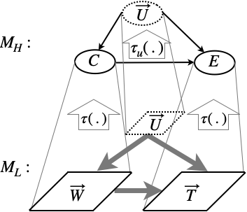
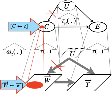
Figure 2: The climate model exemplifies constructive abstraction. Left: $\tau$ and $\tau_{{\cal U}}$ map low-level variables to their high-level counterparts. Right: $\omega_{\tau}$ maps low-level interventions to the high-level intervention. Several different low-level interventions on $\vec{W}$ may correspond to the same intervention on $C$.

3 APPROXIMATE ABSTRACTION

In order to define what it means for one causal model to be an approximation of another, we need a way of measuring the “distance” between causal models. We take a distance function to simply be a function that associates with a pair $(M_{1},M_{2})$ a distance, that is, a non-negative real number. We show how various distance functions on causal models can be defined, starting from a metric $d_{{\cal V}}$ on the state space ${\cal R}({\cal V})$ of a causal model. (Recall that a metric on a space $X$ is a function $d:X\times X\rightarrow\mbox{$I\!\!R$}^{+}$ such that (a) $d(x,x^{\prime})=0$ iff $x=x^{\prime}$, (b) $d(x,y)=d(y,x)$, and (c) $d(x,y)+d(y,z)\geq d(x,z)$.) Such a metric $d_{{\cal V}}$ is typically straightforward to define. Given two states $s_{1}$ and $s_{2}$, we can compare the value of each endogenous variable $X$ in $s_{1}$ and $s_{2}$. The difference in the values determines the distance between $s_{1}$ and $s_{2}$.

The choice of distance function is application-dependent. Different researchers looking at the same data may be interested in different aspects of the data. For example, suppose that the model is defined in terms of 5 variables, $X_{1},\ldots,X_{5}$. $X_{3}$ might be gender and $X_{4}$ might be height. Suppose that we restrict to distance functions that takes the distance between $(x_{1},\ldots,x_{5})$ and $(x_{1}^{\prime},...,x_{5}^{\prime})$ to be of the form $\sqrt{w_{1}(x_{1}-x_{1}^{\prime})^{2}+\cdots+w_{5}(x_{5}-x_{5}^{\prime})^{2}}$, where $w_{1},\ldots,w_{5}$ are weights that represent the importance (to the researcher) of each of these five features. One researcher might not be interested in gender (so doesn’t care if her predictions about gender are incorrect), and thus might take $w_{3}=0$; another researcher might care about gender and not about height, so she might take $w_{3}=1$ and $w_{4}=0$. While, as we shall see, the choice of distance function makes a crucial difference in evaluating the “goodness” of an approximate abstraction, in light of the above, we leave the choice of distance function unspecified.

In the remainder of the paper, we assume that the state space ${\cal R}({\cal V})$ of endogenous variables for each causal model comes with a metric $d_{{\cal V}}$. We provide a number of ways of lifting the metric $d_{{\cal V}}$ on states to a distance function $d$ on models, and then use the distance function to define both approximation and approximate abstraction.

Our intuition for the distance function is based on how causal models are typically used. Specifically, we are interested in how two models compare with regard to the predictions they make about the effects of an intervention. Our intuition is similar in spirit to that behind the notion of structural intervention distance considered by Peters and Bühlmann PB15, although the technical definitions are quite different. (We discuss the exact relationship between our approach and theirs in the next section, in the context of probabilistic models.)

We start with the simplest setting where this intuition can be made precise, one where the models $M_{1}$ and $M_{2}$ differ only with regards to their equations. We say that two models are similar in this case. If two models are similar, then, among other things, we can assume that they have the same metric $d_{{\cal V}}$. In this setting, we can compare the effect of each allowed intervention $\vec{X}\leftarrow\vec{x}$ in the two models. That is, for each context $\vec{u}$, we can compare the states $M_{1}(\vec{u},\vec{X}\leftarrow\vec{x})$ and $M_{2}(\vec{u},\vec{X}\leftarrow\vec{x})$ that arise after performing the intervention $\vec{X}\leftarrow\vec{x}$ in context $\vec{u}$ in each model. We get the desired distance function by taking the worst-case distance between all such states.

Definition 3.1

: Define a distance function $d_{max}$ on pairs of similar models by taking

$$\begin{array}[]{ll}d_{max}(M_{1},M_{2})=\\ \max_{\vec{X}\leftarrow\vec{x}\in{\cal I}\text{, }\vec{u}\in{\cal R}({\cal U})}\{d_{{\cal V}}(M_{1}(\vec{u},\vec{X}\leftarrow\vec{x}),M_{2}(\vec{u},\vec{X}\leftarrow\vec{x}))\}.\end{array}$$

The causal model $M_{1}$ is a $d_{max}$-$\alpha$ approximation of $M_{2}$ if $d_{max}(M_{1},M_{2})\leq\alpha$.  

Thus, $M_{1}$ is a $d_{max}$-$\alpha$ approximation of $M_{2}$ if the predictions of $M_{1}$ are always within $\alpha$ of the predictions of $M_{2}$.

We apply similar ideas to defining approximate abstraction. But now we no longer have a distance function defined on causal models with the same signature. Rather, the distance function $d_{\tau}$ is defined on pairs $(M_{L},M_{H})$ consisting of a low-level and high-level causal model (which, in general, have different signatures), related by a a surjective mapping $\tau$. The idea behind $d_{\tau}$ is that we start with a low-level intervention $\vec{X}\leftarrow\vec{x}$, consider its effects in $M_{L}$, lift this up to $M_{H}$ using $\tau$, and compare this to the effects of $\omega_{\tau}(\vec{X}\leftarrow\vec{x})$ in $M_{H}$.

Definition 3.2

: Fix a surjective map $\tau:{\cal R}({\cal V}_{L})\rightarrow{\cal R}({\cal V}_{H})$. Define the distance function $d_{\tau}$ on pairs of $\tau$-consistent models $(M_{L},M_{H})$ by taking

$$\begin{array}[]{ll}d_{\tau}(M_{L},M_{H})=\min_{\mathrm{\tau_{{\cal U}}\ surjective}}\max_{\vec{X}\leftarrow\vec{x}\in{\cal I}_{L}\text{, }\vec{u}_{L}\in{\cal R}_{L}({\cal U}_{L})}\\ (d_{{\cal V}_{H}}(\tau(M_{L}(\vec{u}_{L},\vec{X}\leftarrow\vec{x})),M_{H}(\tau_{{\cal U}}(\vec{u}_{L}),\omega_{\tau}(\vec{X}\leftarrow\vec{x})))).\end{array}$$

$M_{H}$ is a $\tau$-$\alpha$ approximate abstraction of $M_{L}$ if $d_{\tau}(M_{L},M_{H})\leq\alpha$.  

We take the minimum over all functions $\tau_{\cal U}$ because the function that lifts the low-level contexts up to the high-level contexts does not play a major role. We thus simply focus on the best choice of $\tau_{\cal U}$.

To get an intuition for an approximate abstraction, consider the climate example again. For a low-level intervention $\vec{W}\leftarrow\vec{w}$ and a low-level context $\vec{u}$, there are two ways of lifting their effect to $M_{H}$ (see Fig. 3). The first is to start by applying $M_{L}$ to the context-intervention pair to determine a low-level state $\vec{t}$, and then apply $\tau$ to obtain the high-level state $E=e=\tau(\vec{t})$. (Recall that $M_{L}$ can be viewed as a function from context-intervention pairs to states in ${\cal R}_{L}({\cal V}_{L})$.) The second is to first lift the intervention $\vec{W}\leftarrow\vec{w}$ to ${\cal I}_{H}$, that is, an intervention on $C$, and the context to ${\cal U}_{H}$ by applying $\omega_{\tau}$ and $\tau_{{\cal U}}$. Then we apply $M_{H}(\vec{u}_{H},C\leftarrow c)$, which again gives a high-level endogenous state $e^{\prime}$. We are identifying the degree to which $M_{H}$ approximates $M_{L}$ with the worst-case distance between the two ways of lifting the context-intervention pairs, for an optimal choice of $\tau_{{\cal U}}$.

Figure 3: Approximate abstraction in the climate example. We measure (for the worst-case choice of low-level intervention $\vec{W}\leftarrow\vec{w}$ and context $\vec{u}$) the distance between the values of the variable $E$ obtained by (a) first applying $M_{L}$ to $\vec{u}$ and $\vec{W}\leftarrow\vec{w}$ and then abstracting by applying $\tau$ vs. (b) abstracting the intervention and context (by applying $\omega_{\tau}$ and $\tau_{\cal U}$, respectively) and then applying $M_{H}$.

The following straightforward results show that our notion of approximate abstraction is a sensible generalization of both the notion of an exact abstraction and the notion of approximation between similar models.

Proposition 3.3

: $M_{H}$ is a $\tau$-$0$-approximate abstraction of $M_{L}$ iff $M_{H}$ is a $\tau$-abstraction of $M_{L}$.

Proposition 3.4

: If $M_{1}$ and $M_{2}$ are similar, then $M_{2}$ is a $\mathit{Id}$-$\alpha$-approximate abstraction of $M_{1}$ (where $\mathit{Id}$ is the identity function on ${\cal R}({\cal V})$) iff $M_{2}$ is a $d_{max}$-$\alpha$-approximation of $M_{1}$.

4 APPROXIMATE ABSTRACTION FOR PROBABILISTIC CAUSAL MODELS

A probabilistic causal model $M=(\cal S,{\cal F},{\cal I},\Pr)$ is just a causal model together with a probability $\Pr$ on contexts $\vec{u}$. In this section, we assume that all causal models are probabilistic, and extend the notion of approximation to probabilistic causal models. We again start by considering the simplest setting, where we have probabilistic models that differ only in their equations. We again call such models similar. Now we have several reasonable distance functions.

Definition 4.1

: Define a distance function $d_{max}$ on pairs of similar probabilistic causal models by taking

$$\begin{array}[]{ll}d_{max}(M_{1},M_{2})=\max_{\vec{X}\leftarrow\vec{x}\in{\cal I}}\\ \left(\sum_{\vec{u}\in{\cal R}({\cal U})}\Pr(\vec{u})d_{{\cal V}}(M_{1}(\vec{u},\vec{X}\leftarrow\vec{x}),M_{2}(\vec{u},\vec{X}\leftarrow\vec{x}))\right).\end{array}$$

The probabilistic causal model $M_{1}$ is a $d_{max}$-$\alpha$ approximation of $M_{2}$ if $d_{max}(M_{1},M_{2})\leq\alpha$.  

Here we have just replaced the max over contexts in Definition 3.1 by an expectation over contexts.

But we may not always just be interested in the expected distance. We may, for example, be more concerned with the likelihood of serious prediction differences, and not be too concerned about small differences. This leads to the following definition.

Definition 4.2

: Define a distance function $d_{\beta}$ on pairs of similar probabilistic causal models by taking

$$\begin{array}[]{ll}d_{\beta}(M_{1},M_{2})=\max_{\vec{X}\leftarrow\vec{x}\in{\cal I}}\\ \Pr(\{\vec{u}:d_{{\cal V}}(M_{1}(\vec{u},\vec{X}\leftarrow\vec{x}),M_{2}(\vec{u},\vec{X}\leftarrow\vec{x}))\geq\beta\}.\end{array}$$

The probabilistic causal model $M_{1}$ is a $d_{\beta}$-$\alpha$ approximation of $M_{2}$ if $d_{\beta}(M_{1},M_{2})\leq\alpha$.  

We can now extend these ideas to approximate abstraction. We first extend the definition of $\tau$-abstraction to the probabilistic setting.

Note that we can view $\Pr$ as a probability measure on ${\cal R}({\cal V})$, by taking $\Pr(\vec{v})=\{\vec{u}:M(\vec{u})=\vec{v}\}$. An intervention $\vec{X}\leftarrow\vec{x}$ also induces a probability $\Pr^{\vec{X}\leftarrow\vec{x}}$ on ${\cal R}({\cal V})$ in the obvious way:

$${\Pr}^{\vec{X}\leftarrow\vec{x}}(\vec{v})=\Pr(\{\vec{u}:M(\vec{u},\vec{X}\leftarrow\vec{x})=\vec{v}\}).$$

In the deterministic notion of abstraction, we require that the two high-level states obtained by the two different ways of lifting the effects of a low-level intervention to the high level be equal. In the probabilistic notion, we require that the two different probability distributions obtained by the two ways of lifting an intervention be equal.

Definition 4.3

: $M_{H}$ is a $\tau$-abstraction of $M_{L}$ if $M_{H}$ and $M_{L}$ are $\tau$-consistent and for all interventions $\vec{X}\leftarrow\vec{x}\in{\cal I}_{L}$, we have that $\tau({\Pr}_{L}^{\vec{X}\leftarrow\vec{x}})={\Pr}_{H}^{\omega_{\tau}(\vec{X}\leftarrow\vec{x})}.$  

We can now extend our definitions to the approximate scenario just as we did for deterministic causal models.

Definition 4.4

: Fix a surjective map $\tau:{\cal R}({\cal V}_{L})\rightarrow{\cal R}({\cal V}_{H})$. Define the distance function $d_{\tau}$ on pairs of $\tau$-consistent probabilistic causal models by taking

$$\begin{array}[]{ll}d_{\tau}(M_{L},M_{H})=\min_{\mathrm{\{\tau_{{\cal U}}:\tau_{{\cal U}}(\Pr_{L})=\Pr_{H}\}}}\max_{\vec{X}\leftarrow\vec{x}\in{\cal I}_{L}}\\ (\sum_{\vec{u}_{L}\in{\cal R}_{L}({\cal U}_{L})}\Pr_{L}(\vec{u}_{L})\\ d_{{\cal V}_{H}}(\tau(M_{L}(\vec{u}_{L},\vec{X}\leftarrow\vec{x})),M_{H}(\tau_{{\cal U}}(\vec{u}_{L}),\omega_{\tau}(\vec{X}\leftarrow\vec{x})))).\end{array}$$

$M_{H}$ is a $\tau$-$\alpha$ approximate abstraction of $M_{L}$ if $d_{\tau}(M_{L},M_{H})\leq\alpha$.  

For the climate example this definition implies the following: Suppose we introduce probabilities by specifying distributions over the contexts $\vec{u}_{L}$ and $\vec{u}_{H}$. The resulting probabilistic causal model $(M_{H},Pr_{H})$ is a $\tau$-$\alpha$ approximate abstraction of $(M_{L},Pr_{L})$ if the expectation (in terms of $Pr_{L}$) of the difference between the states $e$ and $e^{\prime}$ of the high-level temperature variable $E$ is less or equal to $\alpha$, where $e$ and $e^{\prime}$ are determined exactly in accordance with the two pathways in Fig. 3, selecting the worst-case intervention $\vec{W}\leftarrow\vec{w}$ and the best case $\tau_{{\cal U}}$.

Analogously to the deterministic case, we have the following straightforward results.

Proposition 4.5

: $M_{H}$ is a $\tau$-$0$-approximate abstraction of $M_{L}$ iff $M_{H}$ is a $\tau$-abstraction of $M_{L}$.

Proposition 4.6

: If $M_{1}$ and $M_{2}$ are similar, then $M_{2}$ is a $Id$-$\alpha$-approximate abstraction of $M_{1}$ iff $M_{2}$ is a $d_{max}$-$\alpha$-approximation of $M_{1}$.

In Definition 4.4 we consider the worst-case low-level intervention to define the distance. In many cases, however, the whole point of an abstraction is to be able to exclude rare low-level boundary cases (e.g., when the ideal gas law is taken to refer only to equilibrium states). Moreover, often the actual manipulations that we can perform are known to us only at the high-level, because the low-level implementation of the intervention is unobservable to us. For example, in setting the room temperature to $70^{\circ}$F we do not generally consider the instantiation of that intervention which superheats one corner of the room and freezes the rest such that the mean kinetic energy works out just right. As Spirtes and Scheines SS04 show, in the absence of any further information, such ambiguous manipulations can be quite problematic. Fortunately, often our knowledge of the mechanism of how a high-level intervention is implemented does give us significant probabilistic information. For example, we might know that the heater has a fan that circulates the air, most likely resulting in relatively uniform distributions of the kinetic energies of the particles.

We capture this information using what we call an intervention distribution.

Definition 4.7

: Given a surjective map $\tau:{\cal R}({\cal V}_{L})\rightarrow{\cal R}({\cal V}_{H})$, an intervention distribution ${\Pr}_{\cal I}$ is a distribution on ${\cal I}_{L}\times{\cal I}_{H}$ such that ${\Pr}_{\cal I}(\vec{X}\leftarrow\vec{x}\mid\vec{Y}\leftarrow\vec{y})>0$ iff $\omega_{\tau}(\vec{X}\leftarrow\vec{x})=\vec{Y}\leftarrow\vec{y}$.  

We think of $\Pr_{\cal I}(\vec{X}\leftarrow\vec{x}\mid\vec{Y}\leftarrow\vec{y})$ as telling us how likely the high-level intervention $\vec{Y}\leftarrow\vec{y}$ is to have been implemented by the low-level intervention $\vec{X}\leftarrow\vec{x}$.

Definition 4.8

: Given a surjective map $\tau:{\cal R}({\cal V}_{L})\rightarrow{\cal R}({\cal V}_{H})$ and an intervention-distribution ${\Pr}_{\cal I}$, the distance function $d_{\tau}^{\Pr_{{\cal I}}}$ on pairs of $\tau$-consistent probabilistic causal models is defined by taking

$$\begin{array}[]{ll}d_{\tau}^{\Pr_{{\cal I}}}(M_{L},M_{H})=\min_{\{\tau_{{\cal U}}:\,\tau_{{\cal U}}(\Pr_{L})=\Pr_{H}\}}\max_{\vec{Y}\leftarrow\vec{y}\in{\cal I}_{H}}\\ (\sum_{\vec{u}_{L}\in{\cal R}_{L}({\cal U}_{L})}\Pr_{L}(\vec{u}_{L})\\ \sum_{\vec{X}\leftarrow\vec{x}\in{\cal I}_{L}}{\Pr}_{{\cal I}}(\vec{X}\leftarrow\vec{x}\mid\vec{Y}\leftarrow\vec{y})\\ d_{{\cal V}_{H}}(\tau(M_{L}(\vec{u}_{L},\vec{X}\leftarrow\vec{x})),M_{H}(\tau_{{\cal U}}(\vec{u}_{L}),\omega_{\tau}(\vec{X}\leftarrow\vec{x})))).\end{array}$$

 

Intuitively, for each high-level intervention $\vec{Y}\leftarrow\vec{y}$, we take the expected distance between the two ways of lifting a low-level intervention to $\vec{Y}\leftarrow\vec{y}$. In computing the expectation, there are two sources of uncertainty: the likelihood of a given context (this is determined by $\Pr_{L}$) and the likelihood on each low-level intervention that maps to $\vec{Y}\leftarrow\vec{y}$ (this is given by $\Pr_{{\cal I}}(\cdot\mid\vec{Y}\leftarrow\vec{y})$). Fig. 4 illustrates the point for the climate example.

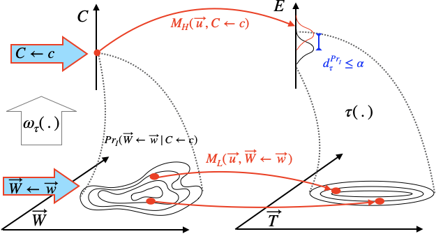
Figure 4: Probabilistic approximate abstraction for the climate example: An intervention on the high-level wind variable $C$ results, given the distribution over contexts $\vec{u}$ (omitted for clarity), in the red distribution over the high-level temperature variable $E$. The intervention $C\leftarrow c$ can be instantiated in the low-level wind map $\vec{W}$ in many ways, according to the intervention distribution $Pr_{{\cal I}}$. Mapping the (manipulated) distribution over $\vec{W}$ using $M_{L}$ results in a distribution over the low-level temperature map $\vec{T}$ that combines uncertainty from $Pr_{{\cal I}}$ and $Pr_{{\cal U}}$. Abstracting this distribution using $\tau$ to $E$ results in the black distribution over $E$. $M_{H}$ is a probabilistic $\tau$-$\alpha$-approximate abstraction of $M_{L}$ if the distance between the expectations of these distributions is less than $\alpha$.

We can also define $d_{\beta}^{\tau}$ and $d_{\beta}^{\tau,\Pr_{{\cal I}}}$ in a manner completely analogous to Definition 4.2. We omit these definitions for reasons of space, but the details should be clear.

It is worth comparing our approach to other approaches to determining the distance between causal models. The more standard way to compare two causal models is to compare their causal graphs. The causal graph is a directed acyclic graph (dag) that has nodes labeled by variables; (the node labeled) $X$ is an ancestor of (the node labeled) $Y$ iff $X\prec Y$. Dags have been compared using what is called the structural Hamming distance (SHD) [Acid and de CamposAcid and de Campos2003], where the SHD between $G$ and $H$ (which are assumed to have an identical set of nodes) is the number of pairs of nodes $(i,j)$ on which $G$ and $H$ differ regarding the edge between $i$ and $j$ (either because one of one of them has an edge and the other does not, or the edges are oriented in different directions). As Peters and Bühlmann PB15 observe, the SHD misses out on some important information in causal networks. In particular, it does not really compare the effect of interventions. They want a notion of distance that takes this into account, as do we. However, they take into account the effect of interventions in a way much closer in spirit to SHD. Roughly speaking, in our language, given two similar causal models $M_{1}$ and $M_{2}$, they count the number of pairs $(X,Y)$ of endogenous variables such that intervening on $X$ leads to a different distribution over $Y$ in $M_{1}$ and $M_{2}$. More formally, let $\Pr^{M,X\leftarrow x}_{Y}$ denote the marginal of $\Pr^{M,X\leftarrow x}$ on the variable $Y$ in model $M$. (Since we want to compare probability distributions in two different models, we add the model to the superscript.) The SID between similar models $M_{1}$ and $M_{2}$ is the number of pairs $(X,Y)$ such that there exists an $x\in{\cal R}(X)$ such that $\Pr^{M_{1},X\leftarrow x}_{Y}\neq\Pr^{M_{2},X\leftarrow x}_{Y}$.

Although SID does compare the predictions that two models make, it differs from our distance functions in several important respects. First, it compares just the effect of interventions on single variables, whereas we allow arbitrary interventions. We believe that it is important to consider arbitrary interventions, since sometimes variables act together, and it takes intervening on more than one variable to distinguish two models. Second, we are interested in how far apart two distributions are, not just the fact that they are different. Finally, we want a definition that applies to models that are not similar, since this is what we need for approximate abstraction.

5 COMPOSING ABSTRACTION AND APPROXIMATION

It can be useful to understand an approximate abstraction as the result of composing an approximation and an abstraction, in some order. For example, we can explain the ideal gas law in terms of thinking of frictionless elastic collisions between particles (this is an approximation to the truth) and then abstracting by replacing the kinetic energy of the particles by their temperature (a measure of average kinetic energy). Here we examine the extent to which an approximate abstraction can be viewed this way. We start with two easy results showing that if we compose an approximation and an abstraction in some order, then we do get an approximate abstraction.

Proposition 5.1

: If $(M_{H},{\cal I}_{H})$ is a $\tau$-abstraction of $(M_{L},{\cal I}_{L})$ and $(M_{H}^{\prime},{\cal I}_{H})$ is a $d_{max}$-$\alpha$-approximation of $(M_{H},{\cal I}_{H})$ then $(M_{H}^{\prime},{\cal I}_{H})$ is a $\tau$-$\alpha$ approximate abstraction of $(M_{L},{\cal I}_{L})$.

In Proposition 5.1 we considered an abstraction followed by an approximation. Things change if we do things in the opposite order; that is, if we consider an approximation followed by an abstraction. For suppose that $M_{L}^{\prime}$ is a $d_{max}$-$\alpha$ approximation of $M_{L}$ and $M_{H}$ is a $\tau$-abstraction of $M_{L}$. Now it is not in general the case that $M_{H}$ is a $d_{\tau}$-$\alpha$-approximate abstraction of $M_{L}^{\prime}$. The problem is that when assessing how good an abstraction $M_{H}$ is of $M_{L}^{\prime}$, we are comparing two high-level states (using $d_{{\cal V}_{H}}$). But when comparing $M_{L}$ to $M_{L}^{\prime}$, we use $d_{{\cal V}_{L}}$. In general, $d_{{\cal V}_{L}}(\vec{v}_{L},\vec{v}_{L}^{\prime})$ and $d_{{\cal V}_{H}}(\tau(\vec{v}_{L}),\tau(\vec{v}_{L}^{\prime}))$ may be unrelated.

Proposition 5.2

: If $(M_{H},{\cal I}_{H})$ is a $\tau$-abstraction of $(M_{L},{\cal I}_{L})$ and $(M_{L},{\cal I}_{L})$ is a $d_{max}$-$\alpha$ approximation of $(M_{L}^{\prime},{\cal I}_{L})$, then $(M_{H},{\cal I}_{H})$ is a $\tau$-$k\alpha$ approximate abstraction of $(M_{L}^{\prime},{\cal I}_{L}^{\prime})$, where $k$ is

$$\begin{array}[]{ll}\max_{\vec{X}\leftarrow\vec{x}\in{\cal I}_{L},\vec{u}_{L}\in{\cal R}_{L}({\cal U}_{L})}\\ \frac{d_{{\cal V}_{H}}(\tau(M_{L}^{\prime}(\vec{u}_{L},\vec{X}\leftarrow\vec{x})),\tau(M_{L}(\vec{u}_{L},\vec{X}\leftarrow\vec{x})))}{d_{{\cal V}_{L}}(M_{L}^{\prime}(\vec{u}_{L},\vec{X}\leftarrow\vec{x}),M_{L}(\vec{u}_{L},\vec{X}\leftarrow\vec{x}))}.\end{array}$$

While composing an approximation and an abstraction gives us an approximate abstraction, the following two examples show that we cannot in general decompose an approximate abstraction into an abstraction composed with an approximation or an approximation composed with an abstraction. Theorem 5.6 below shows that if we restrict ourselves to the constructive case then we can do the former. However, Example 5.4 shows that, even if we restrict to the constructive case, we cannot do the latter.

Example 5.3

: $M_{L}$ has one exogenous variable $U$ and endogenous variables $A$, $B$, and $C$. $M_{H}$ also has one exogenous variable $U$ and endogenous variables $D$ and $E$. All the endogenous variables have range $\{0,1\}$; $U$ has range $\{0\}$. Let $\tau:{\cal R}({\cal V}_{L})\rightarrow{\cal R}({\cal V}_{H})$ be $\tau(a,b,c)=(a\oplus b,b\oplus c)$, where $\oplus$ denotes addition mod 2. The equations for both $M_{L}$ and $M_{H}$ take the form $V=U$ for all variables $V$. ${\cal I}_{L}$ consists of the empty intervention, and interventions $B\leftarrow 1$, $B\leftarrow 0$, $A\leftarrow 1$, and $A\leftarrow 0$. ${\cal I}_{H}$ consists of only the empty intervention. Taking as $d_{{\cal V}_{H}}$ the Euclidean distance, we leave it to the reader to verify that $M_{H}$ is a $\tau$-$\sqrt{2}$ approximate abstraction of $M_{L}$. However, there does not exist any $M_{L}^{\prime}$ that is similar to $M_{L}$ such that $M_{H}$ is a $\tau$-abstraction of $M_{L}^{\prime}$. To see why, note that the only state in $M_{H}$ that arises from applying an intervention is $(0,0)$. Therefore, the only states in $M_{L}$ that can arise from interventions are ones where $a\oplus b=0$ and $b\oplus c=0$. This means that under the intervention $B\leftarrow 0$, we must have $A=0$, and under $B\leftarrow 1$, we must have $A=1$. Therefore $B\prec A$. It also means that under $A\leftarrow 1$ we must have $B=1$ and under $A\leftarrow 0$ we must have $B=0$, so that $A\prec B$. Thus, $M_{H}$ cannot be recursive.  

Example 5.4

: Let $M_{L}$ be the model where ${\cal U}_{L}=\{U\}$, ${\cal V}_{L}=\{X_{1},X_{2},X_{3}\}$, ${\cal R}(X_{i})=\{0,1\}$ for $i=1,2,3$, the equations are $X_{1}=U$, $X_{2}=X_{1}$, and $X_{3}=X_{2}$, and ${\cal I}_{L}$ consists of all interventions such that $X_{1}$ is intervened on iff $X_{3}$ is intervened on. Let $M_{H}$ be the model where ${\cal U}_{H}={\cal U}_{L}=\{U\}$, ${\cal V}_{H}=\{Y_{1},Y_{2}\}$, ${\cal R}(Y_{1})=\{0,1\}\times\{0,1\}$, ${\cal R}(Y_{2})=\{0,1\}$, the equations are $Y_{1}=(U,U)$, $Y_{2}=\mathit{proj}_{1}(Y_{1})$, the first component of $Y_{1}$, and ${\cal I}_{H}$ consists of all interventions. Let $P=\{\{X_{1},X_{3}\},\{X_{2}\}\}$, and $\tau$ is such that $\tau(x_{1},x_{2},x_{3})=((x_{1},x_{3}),x_{2})$. Note that $\tau$ is constructive, that $M_{H}$ and $M_{L}$ are $\tau$-consistent, and that ${\cal I}_{L}={\cal I}_{L}^{\tau}$. Therefore $M_{H}$ is a constructive $\tau$-$\alpha$ approximate abstraction of $M_{L}$ for some $\alpha$ (the value of $\alpha$ depends on the choice of metric $d_{{\cal V}_{H}}$). It is easy to see that $\omega_{\tau}(X_{1}\leftarrow i,X_{3}\leftarrow j)=(Y_{1}\leftarrow(i,j))$ and $\omega_{\tau}(X_{2}\leftarrow k)=(Y_{2}\leftarrow k)$. Note that $M_{L}(0,(X_{1}\leftarrow 1,X_{3}\leftarrow 0))=(1,1,0)$, $M_{L}(0,(X_{1}\leftarrow 0,X_{3}\leftarrow 1))=(0,0,1)$, $M_{L}(0,X_{2}\leftarrow 0)=(0,0,0)$, and $M_{L}(0,X_{2}\leftarrow 1)=(0,1,1)$. For a causal model $M_{H}^{\prime}$ that is similar to $M_{H}$ to be a $\tau$-abstraction of $M_{L}$, there must be some surjection $\tau_{\cal U}$ such that $M_{H}(\tau_{\cal U}(0),Y_{1}\leftarrow(1,0))=((1,0),1)$, $M_{H}(\tau_{\cal U}(0),Y_{1}\leftarrow(0,1))=((0,1),0)$, $M_{H}(\tau_{\cal U}(0),Y_{2}\leftarrow 0)=((0,0),0)$, and $M_{H}(\tau_{\cal U}(0),Y_{2}\leftarrow 1)=((0,1),1)$. It follows that $Y_{1}\prec_{\tau_{\cal U}(0)}Y_{2}$ and $Y_{2}\prec_{\tau_{\cal U}(0)}Y_{1}$. Thus, there is no (recursive) model $M_{H}^{\prime}$ that is a $\tau$-abstraction of $M_{L}$.  

As the following result shows, we can test whether an approximate abstraction can be viewed as the result of composing an abstraction and an approximation.

Theorem 5.5

: If $(M_{H},{\cal I}_{H})$ is a $\tau$-$\alpha$-approximate abstraction of $(M_{L},{\cal I}_{L})$ then the problem of determining whether there exists a model $(M_{H}^{\prime},{\cal I}_{H})$ (resp., $(M_{L}^{\prime},{\cal I}_{L})$) that is similar to $(M_{H},{\cal I}_{H})$ and is an abstraction of $(M_{L},{\cal I}_{L})$ (resp., $(M_{L},{\cal I}_{L})$) is in nondeterministic time polynomial in $|{\cal I}_{L}|\times|{\cal R}_{L}({\cal U}_{L})|$.

There is one important special case where we are guaranteed to be able to find an appropriate intermediate low-level model, and to do so in polynomial time: if the mapping $\tau$ is constructive.

Theorem 5.6

: If $\tau:{\cal R}_{L}({\cal V}_{L})\rightarrow{\cal R}_{H}({\cal V}_{H})$ is constructive, the causal models $(M_{L},{\cal I}_{L})$ and $(M_{H},{\cal I}_{H})$ are $\tau$-consistent, and $(M_{H},{\cal I}_{H})$ is a $\tau$-$\alpha$-approximate abstraction of $(M_{L},{\cal I}_{L})$, then we can find a model $(M^{\prime}_{L},{\cal I}_{L})$ that is similar to $(M_{L},{\cal I}_{L})$, and such that $(M_{H},{\cal I}_{H})$ is a $\tau$-abstraction of $(M^{\prime}_{L},{\cal I}_{L})$ in time polynomial in $|{\cal I}_{L}|\times|{\cal R}_{L}^{\prime}({\cal U}_{L})|$.

As noted earlier, Example 5.4 shows that $\tau$ being constructive does not similarly guarantee the existence of $M_{H}^{\prime}$ in the first half of Theorem 5.5.

6 DISCUSSION AND CONCLUSIONS

By defining notions of abstraction, approximation, and approximate abstraction, we have presented a framework that relates causal models that describe the same system at (possibly) different levels of granularity. While coarser models offer a degree of simplification by omitting details, they also in general entail a loss in accuracy with respect to the fundamental description. Our framework shows how to quantify this loss in accuracy by defining a distance metric that captures the degree to which a more abstract causal model approximates a more detailed causal model. High- and low-level causal models of the same system can vary on almost any dimension. They need not share the same equations, the same variables, or the same interventions. They may involve entirely distinct state spaces. Inevitably, then, there is some degree of choice as to what one deems relevant to the approximation.

Starting with deterministic causal models, we provided a general method for quantifying the “goodness” of an approximate abstraction. As an interesting special case, our approach allows for the comparison of causal models that operate at the same level of detail. We then extended to probabilistic causal models, and considered several different choices for quantifying the distance between models. Finally, we considered the extent to which we could decompose an approximate abstraction into an abstraction and an approximation.

Given the ubiquitous use of causal models in the social and natural sciences that are known not to capture all the causally relevant details, the framework we presented offers a principled way to assess the trade-off between abstraction and accuracy.

Appendix: Proofs

In this appendix, we prove all the results not proved in the main text. We repeat the statements of the results for the reader’s convenience

Proposition 5.1: If $(M_{H},{\cal I}_{H})$ is a $\tau$-abstraction of $(M_{L},{\cal I}_{L})$ and $(M_{H}^{\prime},{\cal I}_{H})$ is a $d_{max}$-$\alpha$-approximation of $(M_{H},{\cal I}_{H})$ then $(M_{H}^{\prime},{\cal I}_{H})$ is a $\tau$-$\alpha$ approximate abstraction of $(M_{L},{\cal I}_{L})$.

Proof: Fix $\vec{X}\leftarrow\vec{x}\in{\cal I}_{L}$ and $\vec{u}_{L}\in{\cal R}_{L}({\cal U}_{L})$. Since $(M_{H},{\cal I}_{H})$ is a $\tau$-abstraction of $(M_{L},{\cal I}_{L})$, there is a mapping $\tau_{{\cal U}}:{\cal U}_{L}\rightarrow{\cal U}_{H}$ such that

$$\tau(M_{L}(\vec{u}_{L},\vec{X}\leftarrow\vec{x}))=M_{H}(\tau_{{\cal U}}(\vec{u}_{L}),\omega_{\tau}(\vec{X}\leftarrow\vec{x})).$$

Since $(M_{H}^{\prime},{\cal I}_{H})$ is a $d_{max}$-$\alpha$ approximation of $(M_{H},{\cal I}_{H})$, we must have

$$\begin{array}[]{ll}&d_{{\cal V}_{H}}(M_{H}^{\prime}(\tau_{{\cal U}}(\vec{u}_{L}),\omega_{\tau}(\vec{X}\leftarrow\vec{x}))),\tau(M_{L}(\vec{u}_{L},\vec{X}\leftarrow\vec{x})))\\ =&d_{{\cal V}_{H}}(M_{H}^{\prime}(\tau_{{\cal U}}(\vec{u}_{L}),\omega_{\tau}(\vec{X}\leftarrow\vec{x}))),\\ &\ \ M_{H}(\tau_{{\cal U}}(\vec{u}_{L}),\omega_{\tau}(\vec{X}\leftarrow\vec{x})))\\ \leq&\alpha.\end{array}$$

Thus, $(M_{H^{\prime}},{\cal I}_{H})$ is a $\tau$-$\alpha$ approximate abstraction of $(M_{L},{\cal I}_{L})$.  

Proposition 5.2: If $(M_{H},{\cal I}_{H})$ is a $\tau$-abstraction of $(M_{L},{\cal I}_{L})$ and $(M_{L},{\cal I}_{L})$ is a $d_{max}$-$\alpha$ approximation of $(M_{L}^{\prime},{\cal I}_{L})$, then $(M_{H},{\cal I}_{H})$ is a $\tau$-$k\alpha$ approximate abstraction of $(M_{L}^{\prime},{\cal I}_{L}^{\prime})$, where $k$ is

$$\begin{array}[]{ll}\max_{\vec{X}\leftarrow\vec{x}\in{\cal I}_{L},\vec{u}_{L}\in{\cal R}_{L}({\cal U}_{L})}\\ \frac{d_{{\cal V}_{H}}(\tau(M_{L}^{\prime}(\vec{u}_{L},\vec{X}\leftarrow\vec{x})),\tau(M_{L}(\vec{u}_{L},\vec{X}\leftarrow\vec{x})))}{d_{{\cal V}_{L}}(M_{L}^{\prime}(\vec{u}_{L},\vec{X}\leftarrow\vec{x}),M_{L}(\vec{u}_{L},\vec{X}\leftarrow\vec{x}))}.\end{array}$$

Proof: Fix $\vec{X}\leftarrow\vec{x}\in{\cal I}_{L}$ and $\vec{u}_{L}\in{\cal R}_{L}({\cal U}_{L})$. Since $(M_{H},{\cal I}_{H})$ is a $\tau$-abstraction of $(M_{L},{\cal I}_{L})$, there is a mapping $\tau_{{\cal U}}:{\cal U}_{L}\rightarrow{\cal U}_{H}$ such that

$$\tau(M_{L}(\vec{u}_{L},\vec{X}\leftarrow\vec{x}))=M_{H}(\tau_{{\cal U}}(\vec{u}_{L}),\omega_{\tau}(\vec{X}\leftarrow\vec{x})).$$

Since $M_{L}^{\prime}$ is a $d_{max}$-$\alpha$ approximation of $M_{L}$, we have that $d_{{\cal V}_{L}}(M_{L}^{\prime}(\vec{u}_{L},\vec{X}\leftarrow\vec{x}),M_{L}(\vec{u}_{L},\vec{X}\leftarrow\vec{x}))\leq\alpha$. By the definition of $k$, we have that $d_{{\cal V}_{H}}(\tau(M_{L}^{\prime}(\vec{u}_{L},\vec{X}\leftarrow\vec{x})),\tau(M_{L}(\vec{u}_{L},\vec{X}\leftarrow\vec{x}))\leq k\alpha$. Thus, $d_{{\cal V}_{H}}(M_{H}(\tau_{{\cal U}}(\vec{u}_{L}),\omega_{\tau}(\vec{X}\leftarrow\vec{x})),\tau(M_{L}(\vec{u}_{L},\vec{X}\leftarrow\vec{x}))\leq k\alpha$. It follows that $(M_{H},{\cal I}_{H})$ is a $\tau$-$k\alpha$ approximate abstraction of $(M_{L}^{\prime},{\cal I}_{L}^{\prime})$.  

To make our results more general, we use the more general interpretation of recursiveness as it appears in [HalpernHalpern2016]. Concretely, this means that the partial order $\preceq$ on the endogenous variables may depend on the context. We write $\preceq_{\vec{u}}$ for the partial order that exists for context $\vec{u}$. (See footnote 2.)

Theorem 5.5: If $(M_{H},{\cal I}_{H})$ is a $\tau$-$\alpha$-approximate abstraction of $(M_{L},{\cal I}_{L})$ and ${\cal U}_{L}$ and ${\cal I}_{L}$ are finite, then the problem of determining whether there exists a model $(M_{H}^{\prime},{\cal I}_{H})$ (resp., $(M_{L}^{\prime},{\cal I}_{L})$) that is similar to $(M_{H},{\cal I}_{H})$ and is an abstraction of $(M_{L},{\cal I}_{L})$ (resp., $(M_{L},{\cal I}_{L})$ is in nondeterministic time polynomial in $|{\cal I}_{L}|\times|{\cal R}_{L}^{\prime}({\cal U}_{L})|$.

Proof: We start with the problem of determining $M_{H}^{\prime}$. Since ${\cal U}_{H}$ and ${\cal U}_{L}$ are finite, there are only finitely many possible surjections from ${\cal U}_{L}$ to ${\cal U}_{H}$. A surjection $\tau_{{\cal U}}$ is potentially high-level compatible with $\tau$ if

1. For all $\vec{X}\leftarrow\vec{x},\ \vec{X}^{\prime}\leftarrow\vec{x}^{\prime}\in{\cal I}_{L}$ and all $\vec{u},\,\vec{u}^{\prime}\in{\cal R}_{L}({\cal U}_{L})$, if $\omega_{\tau}(\vec{X}\leftarrow\vec{x})=\omega_{\tau}(\vec{X}^{\prime}\leftarrow\vec{x}^{\prime})$ and $\tau_{{\cal U}}(\vec{u})=\tau_{{\cal U}}(\vec{u}^{\prime})$, then $\tau(M_{L}(\vec{u}_{L},\vec{X}\leftarrow\vec{x}))=\tau(M_{L}(\vec{u}_{L}^{\prime},\vec{X}^{\prime}\leftarrow\vec{x}^{\prime}))$

2. For all $\vec{u}_{H}\in{\cal R}_{H}({\cal U}_{H})$, there exists a partial order $\prec_{\vec{u}_{H}}$ on the variables in ${\cal V}_{H}$ such that for all $\vec{u}_{L}\in{\cal R}_{L}({\cal U}_{L})$ with $\vec{u}_{H}=\tau_{{\cal U}}(\vec{u}_{L})$, all pairs of interventions $\vec{X}\leftarrow\vec{x}$ and $\vec{X}^{\prime}\leftarrow\vec{x}^{\prime}$ in ${\cal I}_{L}$, and all variables $Y\in{\cal V}_{H}$ whose value differs in $\tau(M_{L}(\vec{u}_{L},\vec{X}\leftarrow\vec{x}))$ and $\tau(M_{L}(\vec{u}_{L},\vec{X}^{\prime}\leftarrow\vec{x}^{\prime}))$, there exists a variable $Z$ such that $Z\preceq_{\vec{u}_{H}}Y$ (i.e., $Z\prec_{\vec{u}_{H}}Y$ or $Z=Y$) and different values in $\omega_{\tau}(\vec{X}\leftarrow\vec{x})$ and $\omega_{\tau}(\vec{X}^{\prime}\leftarrow\vec{x}^{\prime})$ or $Z$ is assigned a value in one of $\omega_{\tau}(\vec{X}\leftarrow\vec{x})$ and $\omega_{\tau}(\vec{X}^{\prime}\leftarrow\vec{x}^{\prime})$ and not in the other.

We claim that $\tau_{{\cal U}}$ is potentially high-level compatible with $\tau$ iff there exists a (recursive) causal model $(M_{H}^{\prime},{\cal I}_{H})$ such that, for all contexts $\vec{u}_{L}\in{\cal R}_{L}({\cal U}_{L})$ and interventions $\vec{X}\leftarrow\vec{x}\in{\cal I}_{L}$, we have

$$\tau(M_{L}(\vec{u}_{L},\vec{X}\leftarrow\vec{x}))=M_{H}^{\prime}(\tau_{{\cal U}}(\vec{u}_{L}),\omega_{\tau}(\vec{X}\leftarrow\vec{x})).$$ (1)

It is easy to see that if PC1 or PC2 do not hold for $\tau_{{\cal U}}$, then there can be no (recursive) causal model $(M_{H}^{\prime},{\cal I}_{H})$ satisfying (1). For the converse, to build the model $M_{H}^{\prime}$, we have to specify the equations for each variable in such a way that $\prec_{\vec{u}_{H}}$ really is the partial order showing the dependence on variables in context $\vec{u}_{H}$. Say that a high-level state $\vec{v}_{H}\in{\cal R}_{H}({\cal V}_{H})$ is constructible for $\vec{u}_{H}$ and $Y\in{\cal V}_{H}$ if $\vec{v}_{H}=\tau(M_{L}(\vec{u}_{L},\vec{X}\leftarrow\vec{x}))$ for some intervention $\vec{X}\leftarrow\vec{x}\in{\cal I}_{L}$ and context $\vec{u}_{L}\in{\cal R}_{L}({\cal U}_{L})$ such that $\tau_{\cal U}(\vec{u}_{L})=\vec{u}_{H}$ and $\omega_{\tau}(\vec{X}\leftarrow\vec{x})$ does not include an intervention on $Y$. Each high-level state $\vec{v}_{H}$ constructible for $\vec{u}_{H}$ and $Y\in{\cal V}_{H}$ determines one output of $F^{\prime}_{Y}$ in context $\vec{u}_{H}$ in the obvious way. Specifically, if $F^{\prime}_{Y}$ gets as arguments $\vec{u}_{H}$ and the values of the variables other than $Y$ in $\vec{v}_{H}$, then it must output the value of $Y$ in $\vec{v}_{H}$. Note that it follows from PC2 that for the values of $F^{\prime}_{Y}$ so defined, if two inputs to $F^{\prime}_{Y}$ agree on the values of all variables $Z$ such that $Z\prec_{\vec{u}_{H}}Y$, they will agree on the value of $Y$. We want to extend all the equations $F^{\prime}_{Y}$ such that this continues to be true. This is straightforward.

Fix $\vec{u}_{H}$. We define $F_{Y}^{\prime}$ when the context is $\vec{u}_{H}$ for all variables $Y\in{\cal V}_{H}$ as follows. If $Y$ has no predecessors in the $\prec_{\vec{u}_{H}}$ order, then it gets the same value in all the constructible states for context $\vec{u}_{H}$. We extend $F_{Y}^{\prime}$ so that $Y$ gets that value no matter what the values of the endogenous variables other than $Y$ are in context $\vec{u}_{H}$. Similarly, if $Z_{1},\ldots,Z_{k}$ are the variables that precede $Y$ in the $\prec_{\vec{u}_{H}}$ order, and $(Z_{1},\ldots,Z_{k})=(z_{1},\ldots,z_{k})$ appears in some constructible state for $\vec{u}_{H}$ then, by PC2, $Y$ has the same value in all constructible states for $\vec{u}_{H}$ where $(Z_{1},\ldots,Z_{k})=(z_{1},\ldots,z_{k})$. We extend $F_{Y}^{\prime}$ so that $Y$ has that value for all inputs where $(Z_{1},\ldots,Z_{k})=(z_{1},\ldots,z_{k})$ and the context is $\vec{u}_{H}$. If there is no constructible state where $(Z_{1},\ldots,Z_{k})=(z_{1},\ldots,z_{k})$, then we just pick a fixed value $y\in{\cal R}_{H}(Y)$ and take $F_{Y}^{\prime}$ to be $y$ for all inputs where $(Z_{1},\ldots,Z_{k})=(z_{1},\ldots,z_{k})$ and the context is $\vec{u}_{H}$. It is clear by construction that this definition has the desired properties.

We conclude this part of the proof by observing that checking that PC1 holds can be done in time polynomial in $|{\cal I}_{L}|\times|{\cal R}_{L}({\cal U}_{L})|$, and for a fixed ordering $\prec_{\tau_{{\cal U}}}$, PC2 can be checked in time polynomial in $|{\cal I}_{L}|\times|{\cal R}_{L}({\cal U}_{L})|$. Thus, we can determine whether there exists a model $(M_{H}^{\prime},{\cal I}_{H})$ that is an abstraction of $(M_{L},{\cal I}_{L})$ and differs from $(M_{H},{\cal I}_{H})$ only in the equations by guessing $\tau_{{\cal U}}$ and a collection of partial orders $\prec_{\vec{u}_{H}}$, one for each high-level context, and confirming that PC1 and PC2 hold. Thus, this can be done in nondeterministic time polynomial in $|{\cal I}_{L}|\times|{\cal R}_{L}({\cal U}_{L})|$.

The algorithm for determining $(M_{L}^{\prime},{\cal I}_{L})$ is very similar in spirit. A surjection $\tau_{{\cal U}}:{\cal R}_{L}({\cal V}_{L})\rightarrow{\cal R}_{H}({\cal V}_{H})$ and a function $f:{\cal R}({\cal U}_{L})\times{\cal I}_{L}\rightarrow{\cal R}({\cal V}_{L})$ are potentially low-level compatible with $\tau$ if they satisfy:

1. For all $\vec{X}\leftarrow\vec{x},\ \vec{X}^{\prime}\leftarrow\vec{x}^{\prime}\in{\cal I}_{L}$ and all $\vec{u},\,\vec{u}^{\prime}\in{\cal R}_{L}({\cal U}_{L})$, if $\omega_{\tau}(\vec{X}\leftarrow\vec{x})=\omega_{\tau}(\vec{X}^{\prime}\leftarrow\vec{x}^{\prime})$ and $\tau_{{\cal U}}(\vec{u})=\tau_{{\cal U}}(\vec{u}^{\prime})$, then $\tau(f(\vec{u}_{L},\vec{X}\leftarrow\vec{x}))=\tau(f(\vec{u}_{L}^{\prime},\vec{X}^{\prime}\leftarrow\vec{x}^{\prime}))$

2. For all $\vec{u}_{L}\in{\cal R}_{L}({\cal U}_{L})$, there exists a partial order $\prec_{\vec{u}_{L}}$ on the variables in ${\cal V}_{L}$ such that for all interventions $\vec{X}\leftarrow\vec{x}$ and $\vec{X}^{\prime}\leftarrow\vec{x}^{\prime}$ in ${\cal I}_{L}$, and all variables $Y\in{\cal V}_{L}$ whose value differs in $f(\vec{u}_{L},\vec{X}\leftarrow\vec{x})$ and $f(\vec{u}_{L},\vec{X}^{\prime}\preceq_{\vec{u}_{L}}Y$ and either $Z$ gets different values in $\vec{X}\leftarrow\vec{x}$ and $\vec{X}^{\prime}\leftarrow\vec{x}^{\prime}$ or $Z$ is assigned a value in one of $\vec{X}\leftarrow\vec{x}$ and $\vec{X}^{\prime}\leftarrow\vec{x}^{\prime}$ and not in the other.

Essentially, $f(\vec{u}_{L},\vec{X}\leftarrow\vec{x})$ is playing the same role in PC2^′ as $M_{L}(\vec{u}_{L},\vec{X}\leftarrow\vec{x})$ played in PC2.

We now claim that $\tau_{{\cal U}}:{\cal R}_{L}^{\prime}({\cal V}_{L}^{\prime})\rightarrow{\cal R}_{H}({\cal V}_{H})$ and $f:{\cal R}({\cal U}_{L}^{\prime})\times{\cal I}_{L}^{\prime}\rightarrow{\cal R}({\cal V}_{L}^{\prime})$ are potentially low-level compatible with $\tau$ iff there exists a (recursive) causal model $(M_{L}^{\prime},{\cal I}_{L})$ such that for all contexts $\vec{u}_{L}\in{\cal R}_{L}({\cal U}_{L})$ and interventions $\vec{X}\leftarrow\vec{x}\in{\cal I}_{L}$, we have $M_{L}^{\prime}(\vec{u}_{L},\vec{X}\leftarrow\vec{x}))=f(\vec{u}_{L},\vec{X}\leftarrow\vec{x}))$ and

$$\tau(M_{L}^{\prime}(\vec{u}_{L},\vec{X}\leftarrow\vec{x}))=M_{H}(\tau_{{\cal U}}(\vec{u}_{L}),\omega_{\tau}(\vec{X}\leftarrow\vec{x})).$$

The argument is almost identical to that given above for the first part, so we omit it here.

Thus, to determine whether there exists an appropriate model $(M_{L}^{\prime},{\cal I}_{L})$, we simply need to guess $f$, $\tau_{\cal U}$, and $\prec_{\vec{u}_{L}}$ for all $\vec{u}_{L}\in{\cal R}_{L}({\cal U}_{L})$ and verify that PC1^′ and PC2^′ hold.  

Theorem 5.6: If $\tau:{\cal R}_{L}({\cal V}_{L})\rightarrow{\cal R}_{H}({\cal V}_{H})$ is constructive, the causal models $(M_{L},{\cal I}_{L})$ and $(M_{H},{\cal I}_{H})$ are $\tau$-consistent, and $(M_{H},{\cal I}_{H})$ is a $\tau$-$\alpha$-approximate abstraction of $(M_{L},{\cal I}_{L})$, then we can find a model $(M^{\prime}_{L},{\cal I}_{L})$ that is similar to $(M_{L},{\cal I}_{L})$, and such that $(M_{H},{\cal I}_{H})$ is a $\tau$-abstraction of $(M^{\prime}_{L},{\cal I}_{L})$ in time polynomial in $|{\cal I}_{L}|\times|{\cal R}_{L}^{\prime}({\cal U}_{L})|$.

Proof: Whereas in the proof of the second half in Theorem 5.5 we had to guess $\tau_{\cal U}$ and $f$, here we can construct them efficiently. Indeed, we can take $\tau_{\cal U}$ to be an arbitrary surjection from ${\cal U}_{L}$ to ${\cal U}_{H}$.

To define $f$, suppose that ${\cal V}_{H}=\{Y_{1},\ldots,Y_{n}\}$ and $P_{\tau}=\{\vec{Z}_{1},\ldots,\vec{Z}_{n+1}\}$ is the partition that makes $\tau$ constructive (as in Definition 2.6).

In constructing $f(\vec{u}_{L},\vec{X}\leftarrow\vec{x})$, we split the intervention $\vec{X}\leftarrow\vec{x}$ into two parts: an intervention on variables in $\vec{Z}_{1}\cup\ldots\cup\vec{Z}_{n}$ and an intervention on variables in $\vec{Z}_{n+1}$. How $f$ works in the former case is determined by translating the intervention to $M_{H}$. Interventions on variables in $\vec{Z}_{n+1}$ are treated specially. An intervention $V\leftarrow v$ on a variable $V\in\vec{Z}_{n+1}$ just sets $V$ to $v$, and does not affect any other variables. In more detail, we proceed as follows.

Note that $\tau$ is also a surjection from ${\cal R}_{L}(\vec{Z}_{1}\cup\ldots\cup\vec{Z}_{n})$ to ${\cal R}_{H}({\cal V}_{H})$, since the variables in $\vec{Z}_{n+1}$ are ignored by $\tau$. Thus, there is a right inverse $\tau^{-1}:{\cal R}_{H}({\cal V}_{H})\rightarrow{\cal R}_{L}(\vec{Z}_{1}\cup\ldots cup\vec{Z}_{n})$ (so that $\tau\circ\tau^{-1}$ is the identity function on ${\cal R}_{H}({\cal V}_{H})$). There are, in general, many such left inverses, but given $\tau$, we can find a left inverse in time polynomial $|{\cal R}({\cal U}_{L})|$.

Fix a setting $\vec{z}_{n+1}^{*}$ for the variables in $\vec{Z}_{n+1}$. Given an intervention $\vec{X}\leftarrow\vec{x}$, let $\vec{X}^{\dagger}$ be the subset of variables in $\vec{X}$ that are in $\vec{Z}_{1}\cup\ldots\cup\vec{Z}_{n}$, and let $\vec{X}^{\dagger\dagger}$ be the subset of variables in $\vec{X}$ that are in $\vec{Z}_{n+1}$. Let $\vec{x}^{\dagger}$ and $\vec{x}^{\dagger\dagger}$ be the restrictions of $\vec{x}$ to $\vec{X}^{\dagger}$ and $\vec{X}^{\dagger\dagger}$, respectively. Define

$$\begin{array}[]{ll}f(\vec{u}_{L},\vec{X}\leftarrow\vec{x})=\\ (\tau^{-1}(M_{H}(\tau_{\cal U}(\vec{u}_{L}),\omega_{T}(\vec{X}^{\dagger}\leftarrow\vec{x}^{\dagger}))),\vec{z}_{n+1}^{*}[\vec{X}^{\dagger\dagger}=\vec{x}^{\dagger\dagger}]),\end{array}$$

where $\vec{z}_{n+1}^{*}[\vec{X}^{\dagger\dagger}=\vec{x}^{\dagger\dagger})]$ is the tuple that results from $\vec{z}_{n+1}^{*}$ by setting the values of the variables in $\vec{X}^{\dagger\dagger}$ to $\vec{x}^{\dagger\dagger}$.

We first check PC1^′. Suppose that $\vec{X}\leftarrow\vec{x},\ \vec{X}^{\prime}\leftarrow\vec{x}^{\prime}\in{\cal I}_{L}$, $\vec{u}_{L},\,\vec{u}_{L}^{\prime}\in{\cal R}_{L}({\cal U}_{L})$, $\omega_{\tau}(\vec{X}\leftarrow\vec{x})=\omega_{\tau}(\vec{X}^{\prime}\leftarrow\vec{x}^{\prime})$, and $\tau_{{\cal U}}(\vec{u}_{L})=\tau_{{\cal U}}(\vec{u}_{L}^{\prime})$. Then, using the same notation as above and just writing “$\ldots$” for the component of the state describing the values of the variables in $\vec{Z}_{n+1}$, since these values are ignored by $\tau$, we have that

$$\begin{array}[]{ll}&\tau(f(\vec{u}_{L},\vec{X}\leftarrow\vec{x}))\\ =&\tau(\tau^{-1}(M_{H}(\tau_{{\cal U}}(\vec{u}_{L}),\omega_{\tau}(\vec{X}^{\dagger}\leftarrow\vec{x}^{\dagger}))),\ldots)\\ =&\tau(\tau^{-1}(M_{H}(\tau_{{\cal U}}(\vec{u}^{\prime}_{L}),\omega_{\tau}((\vec{X}^{\prime})^{\dagger}\leftarrow(\vec{x}^{\prime})^{\dagger}))),\ldots)\\ =&\tau(f(\vec{u}^{\prime}_{L},\vec{X}^{\prime}\leftarrow\vec{x}^{\prime})).\end{array}$$

To see that PC2^′ holds, fix $\vec{u}_{L}\in{\cal R}_{L}({\cal U}_{L})$. Suppose that ${\cal V}_{H}=\{Y_{1},\ldots,Y_{n}\}$ and $P_{\tau}=\{\vec{Z}_{1},\ldots,\vec{Z}_{n+1}\}$ is the partition that makes $\tau$ constructive (as in Definition 2.6). Since $M_{H}$ is a recursive causal model, there exists a partial order $\prec_{\tau_{{\cal U}}(\vec{u}_{L})}$ on the variables in ${\cal V}_{H}$ such that if $Y_{i}$ depends on $Y_{j}$ in context $\tau_{{\cal U}}(\vec{u}_{L})$, then $Y_{j}\prec_{\tau_{{\cal U}}(\vec{u}_{L})}Y_{i}$. Define $\prec_{\vec{u}_{L}}$ so that $X\prec_{\vec{u}_{L}}X^{\prime}$ iff for some $i$ and $j$, $X\in Z_{j}$, $X^{\prime}\in Z_{i}$, and $Y_{j}\prec_{\tau_{{\cal U}}(\vec{u}_{L})}Y_{i}$. (Note that this means that the variables in $\vec{Z}_{n+1}$ are incomparable to all the rest.)

We now show that this choice of $\prec_{\vec{u}_{L}}$ satisfies PC2^′. Suppose that $\vec{X}\leftarrow\vec{x}$ and $\vec{X}^{\prime}\leftarrow\vec{x}^{\prime}$ in ${\cal I}_{L}$, and the value of $V\in{\cal V}_{L}$ differs in $f(\vec{u}_{L},\vec{X}\leftarrow\vec{x})$ and $f(\vec{u}_{L},\vec{X}^{\prime}\leftarrow\vec{x}^{\prime})$.

If $V\in\vec{Z}_{n+1}$, then it must be the case that $V$ is in $\vec{X}$ or $\vec{X}^{\prime}$. On the other hand, if $V\in\vec{Z}_{i}$ for some $i\leq n$, then the value of $Y_{i}$ differs in $M_{H}(\tau_{{\cal U}}(\vec{u}_{L}),\omega_{\tau}(\vec{X}\leftarrow\vec{x}))$ and $M_{H}(\tau_{{\cal U}}(\vec{u}_{L}),\omega_{\tau}(\vec{X}^{\prime}\leftarrow\vec{x}^{\prime}))$. Therefore, there exists a variable $Y_{j}\in{\cal V}_{H}$ such that $Y_{j}\prec_{\tau_{{\cal U}}(\vec{u}_{L})}Y_{i}$ and either $Y_{j}$ gets different values in $\omega_{\tau}(\vec{X}\leftarrow\vec{x})$ and $\omega_{\tau}(\vec{X}^{\prime}\leftarrow\vec{x}^{\prime})$ or $Y_{j}$ is assigned a value in one of $\omega_{\tau}(\vec{X}\leftarrow\vec{x})$ and $\omega_{\tau}(\vec{X}^{\prime}\leftarrow\vec{x}^{\prime})$ and not in the other. By definition, this means that for all variables $W\in\vec{Z}_{j}$, we have that $W\prec_{\vec{u}_{L}}V$. Furthermore, at least one of these variables $W$ either gets different values in $\vec{X}\leftarrow\vec{x}$ and $\vec{X}^{\prime}\leftarrow\vec{x}^{\prime}$, or is assigned a value in one of $\vec{X}\leftarrow\vec{x}$ and $\vec{X}^{\prime}\leftarrow\vec{x}^{\prime}$ and not in the other.

This concludes the proof.  

Acknowledgements

Beckers was supported by the grant ERC-2013- CoG project REINS 616512. Eberhardt was supported in part by NSF grants 1564330 and BCS-1845958, and HRGC grant 13601017. Halpern was supported in part by NSF grants IIS-1703846 and IIS-1718108, ARO grant W911NF-17-1-0592, and a grant from the Open Philanthropy project. We thank the UAI reviewers for many useful comments.

References

• [\citeauthoryearAcid and de CamposAcid and de Campos2003] Acid, S. and L. M. de Campos (2003). Searching for Bayesian network structures in the space of restricted acyclic partially directed graphs. Journal of A.I. Research 18, 445–490.
• [\citeauthoryearBeckers and HalpernBeckers and Halpern2019] Beckers, S. and J. Y. Halpern (2019). Abstracting causal models. In Proc. Thirty-Third AAAI Conference on Artificial Intelligence (AAAI-19). The full version is available at arxiv.org/abs/1812.03789.
• [\citeauthoryearBoutilier, Friedman, Goldszmidt, and KollerBoutilier et al.1996] Boutilier, C., N. Friedman, M. Goldszmidt, and D. Koller (1996). Context-specific independence in Bayesian networks. In Proc. Twelfth Conference on Uncertainty in Artificial Intelligence (UAI ’96), pp.  115–123.
• [\citeauthoryearChalupka, Bischoff, Perona, and EberhardtChalupka et al.2016] Chalupka, K., T. Bischoff, P. Perona, and F. Eberhardt (2016). Unsupervised discovery of El Niño using causal feature learning on microlevel climate data. In Proc. 32nd Conference on Uncertainty in Artificial Intelligence (UAI 2016), pp.  72–81.
• [\citeauthoryearHalpernHalpern2016] Halpern, J. Y. (2016). Actual Causality. Cambridge, MA: MIT Press.
• [\citeauthoryearHalpern and PearlHalpern and Pearl2005] Halpern, J. Y. and J. Pearl (2005). Causes and explanations: a structural-model approach. Part I: Causes. British Journal for Philosophy of Science 56(4), 843–887.
• [\citeauthoryearPeters and BühlmannPeters and Bühlmann2015] Peters, J. and P. Bühlmann (2015). Structural intervention distance (SID) for evbaluating causal graphs. Neural Computation 27(3), 725–747.
• [\citeauthoryearRubenstein, Weichwald, Bongers, Mooij, Janzing, Grosse-Wentrup, and SchölkopfRubenstein et al.2017] Rubenstein, P. K., S. Weichwald, S. Bongers, J. M. Mooij, D. Janzing, M. Grosse-Wentrup, and B. Schölkopf (2017). Causal consistency of structural equation models. In Proc. 33rd Conference on Uncertainty in Artificial Intelligence (UAI 2017).
• [\citeauthoryearSpirtes and ScheinesSpirtes and Scheines2004] Spirtes, P. and R. Scheines (2004). Causal inference of ambiguous manipulations. Philosophy of Science 71, 833–845.