Entanglement dynamics of two mesoscopic objects with gravitational interaction

Abstract

We analyse the entanglement dynamics of the two particles interacting through gravity in the recently proposed experiments aiming at testing quantum signatures for gravity [Phy. Rev. Lett 119, 240401 & 240402 (2017)]. We consider the open dynamics of the system under decoherence due to the environmental interaction. We show that as long as the coupling between the particles is strong, the system does indeed develop entanglement, confirming the qualitative analysis in the original proposals. We show that the entanglement is also robust against stochastic fluctuations in setting up the system. The optimal interaction duration for the experiment is computed. A condition under which one can prove the entanglement in a device-independent manner is also derived.

I Introduction

The unification of quantum mechanics and general relativity has been perceived as one of the most important open problems of modern physics. Although a substantial theoretical effort has been made, there is not yet an agreement on a single theory of quantum gravity Kiefer (2012). One of the main difficulties of the field is the lack of experimental support Kiefer (2012). As a result, in recent years a number of proposals for searching the signature of quantum gravity in various contexts have been made Hossenfelder (2018). Among these proposals, a simple one making use of recent advances in manipulating mesoscopic quantum mechanical systems was proposed by Bose et al. Bose et al. (2017), and independently by Marletto and Vedral Marletto and Vedral (2017). The proposed experiment has been referred to as the ‘BMV experiment’ Christodolou and Rovelli (2018a).

We consider here a slightly different version of the BMV experiment, see Figure 1(a). Two mesoscopic particles of masses $m_{1}$ and $m_{2}$ are placed at distance $d$ from each other. Each particle is then split into a superposition of two positions that are separated by a distance $L$ orthogonally to their initial separation. Based on recent advances in setting up mesoscopic systems in superposition Bose and Morley (2018); Carney et al. (2018); Howl et al. (2017); Marshman et al. (2018); Qvarfort et al. (2018); Pino et al. (2018), the authors of Ref. Bose et al. (2017) suggested as physically relevant quantities $m_{1}\approx m_{2}\approx 10^{-8}\mathrm{kg}$, $d\approx 200\mathrm{\mu m}$, and we can assume $L\gg d$.

In the original proposal Bose et al. (2017), the particles are split into superpositions of positions in the same direction as their initial separation, see Figure 1(b). They thus have strong gravitational interaction only when the first particle is on the right, while the second particle is on the left. In this current setup the particles interact strongly whenever they are on the same side (left or right). Experimentally, it might be more challenging to setup the system in this symmetric configuration; in particular, one may have to introduce a thin film between the particles to keep the distance constant. We note that a thin film however may have an additional advantage. It could help prevent taming interactions due to the van der Waals or the Casimir effects, which has been an obstacle for the original setup (Bose and Morley, 2018). For convenience, we analyse this symmetric setup, but the analysis can be easily adapted to the original proposal.

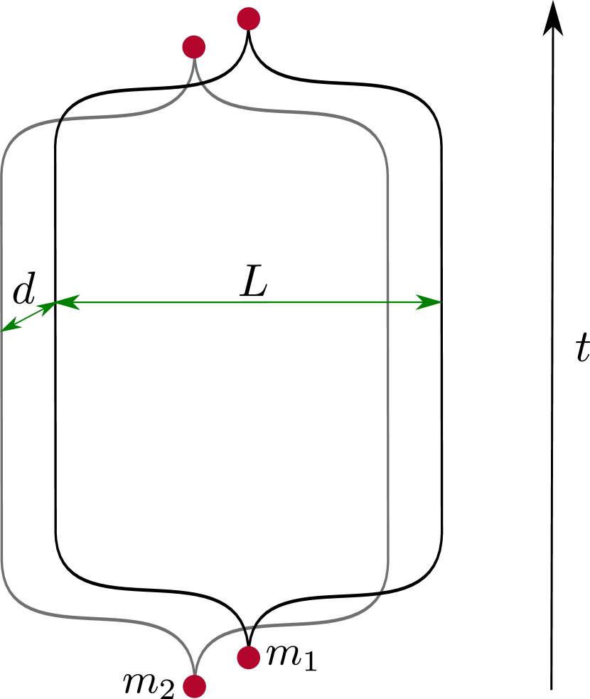
(a)

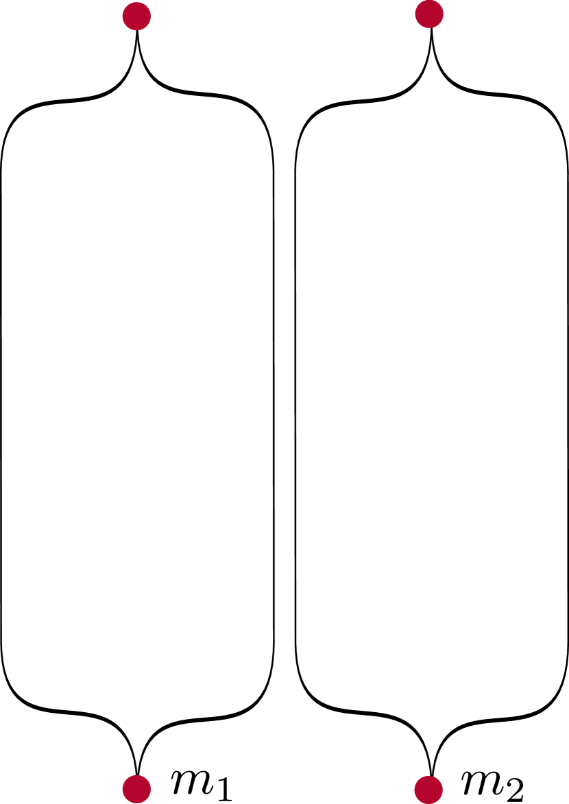
(b)

Figure 1: The BMV experiment. (a) The symmetric setup: two particles are initially at distance $d$ from each other. Each of the particle is then split into a superposition of two positions at distance $L$ from each other in the direction orthogonal to their initial separation. Due to their gravitational interaction the particles are expected to be entangled over time. (b) The original setup: the particles are split into superpositions in parallel to their initial separation.

Formally, the system can be modelled as a pair of spins, where states $\left|\uparrow\right\rangle$ and $\left|\downarrow\right\rangle$ can be identified with the particles being on the left and right, respectively. Due to the gravitational interaction between the particles, if both particles are on the same sides ($\left|\uparrow\uparrow\right\rangle$ or $\left|\downarrow\downarrow\right\rangle$), the energy of the system is $-Gm_{1}m_{2}/d$, with $G$ being the gravitational constant. On the other hand, if they are on the opposite sides ($\left|\uparrow\downarrow\right\rangle$ or $\left|\downarrow\uparrow\right\rangle$), the energy is given by $-Gm_{1}m_{2}/\sqrt{L^{2}+d^{2}}$. Therefore, upto an irrelevant additive constant, the Hamiltonian can be modelled by

$$H=-\frac{\Delta}{2}\sigma_{z}\otimes\sigma_{z},$$ (1)

where $\sigma_{z}$ is one of the usual Pauli matrices and

$$\Delta=Gm_{1}m_{2}\left(\frac{1}{d}-\frac{1}{\sqrt{L^{2}+d^{2}}}\right).$$ (2)

Under the evolution induced by this Hamiltonian, particles that are first given in the superpositions of being left and right, $\left|+\right\rangle\left|+\right\rangle$, where $\left|+\right\rangle=(\left|\uparrow\right\rangle+\left|\downarrow\right\rangle)/\sqrt{2}$, should evolve into an entangled state. Provided one can preserve the coherence of the system long enough, such entanglement is expected to be observable Bose et al. (2017). In the actual physical setting, each particle carries an additional two-level degree of freedom, which is then correlated with its positions (left or right) during the spliting Bose et al. (2017). The result is that, after merging their superpositions, the entanglement in the particle positions is eventually transferred to the entanglement between these additional degrees of freedom and can be directly measured.

The entanglement between the particles has been argued to be an evidence that the gravitational field is a quantum mechanical system Bose et al. (2017); Marletto and Vedral (2017). While this claim is still a subject of debate Hall and Reginatto (2018); Anastopoulos and Hu (2018); Reginatto and Hall (2018); Christodolou and Rovelli (2018a, b), we do believe that the ability to entangle particles via their gravitational interaction would greatly advance our understanding of the interface between quantum mechanics and gravity.

Let $T$ be the decoherence time, the authors of Ref. Bose et al. (2017) argued that the necessary condition to observe the entanglement is

$$(\Delta T)/\hbar\sim\mathcal{O}(1).$$ (3)

While this qualitative estimate is plausible, it is still important to analyse the noisy dynamics of the system in detail to pinpoint the precise condition under which entanglement between the particles can be observed. Here we analyse the details of the decoherence dynamics of the system. More importantly, we also consider fluctuations of the experimental parameters. These stochastic fluctuations in setting the parameters in the proposed experiments imply that one has to average over the obtained entangled states from run to run of the experiment, which results in a reduction of entanglement in the averaged state. While so far this has not been considered, it is also crucial to the experiment, since entanglement can only be verified statistically through multiple runs of the experiment. Our analysis shows that the entanglement is rather robust. More precisely, we show that the entanglement indeed develops as long as $\Delta T/\hbar>1$ if the fluctuations in setting the experimental parameters can be neglected. Moreover, we show that moderate stochastic errors in the experiment can also be tolerated. We discuss the optimal interaction duration for the particles while they are in the superposition state and find a condition under which entanglement can be detected in a device-independent manner.

II The decoherence dynamics of the system

The superposition of the positions of the particles is suppressed in the long time limit because of the environmental interaction. This is known as the decoherence process, which gives rise to our classical notion of position Schlosshauer (2007). While the details of the decoherence process depend on the details of the environment, the system under consideration is sufficiently simple that it can be analysed with some minimal assumptions of the decoherence theory. Indeed, due to decoherence the system decays into a mixed state of positions (and not any other basis), so one can assume that the environment couples only to the position operator of the particles, which is $\sigma_{z}$ in this case Schlosshauer (2007). The coupling Hamiltonian between one particle and the environment can be written generally as

$$H_{D}\propto\sigma_{z}\otimes R,$$ (4)

where $R$ is an operator acting on the environment. This environmental coupling Hamiltonian (4) is such that if the initial reduced state of the particle is given by a $(2\times 2)$ density matrix $a$, it will evolve in a way that its diagonal elements are constant, while its off-diagonal elements decay over time Schlosshauer (2007). Assuming an exponential decay of the off-diagonal elements (known as coherence elements) for specificity, the state of the particle state at time $t$ is given by

$$\rho_{1}(t)=\begin{pmatrix}a_{11}&a_{12}e^{-t}\\ a_{21}e^{-t}&a_{22}\end{pmatrix},$$ (5)

where we have used the dimensionless time $t$, defined by the physical time divided by the decoherence time $T$. While this exponential decaying of coherence is the case for the position decoherence due to the enviromental scattering by photons or air molecules Schlosshauer (2007), other types of decoherence dynamics can also be considered with minimal adaptation.

For the system of two particles without mutual interaction, we assume that their decoherence are independent from each other. If the system is first given in the state $a\otimes b$, where $a$ and $b$ are $(2\times 2)$ density matrices of the first and the second particle, respectively, the density matrix of the whole system at time $t$ is then

$$\begin{pmatrix}a_{11}&a_{12}e^{-t}\\ a_{21}e^{-t}&a_{22}\end{pmatrix}\otimes\begin{pmatrix}b_{11}&b_{12}e^{-t}\\ b_{21}e^{-t}&b_{22}\end{pmatrix}.$$ (6)

By linearity, the two-particle system first given in a $(4\times 4)$ density matrix $c$ then evolves to

$$\begin{pmatrix}c_{11}&c_{12}e^{-t}&c_{13}e^{-t}&c_{14}e^{-2t}\\ c_{21}e^{-t}&c_{22}&c_{23}e^{-2t}&c_{24}e^{-t}\\ c_{31}e^{-t}&c_{32}e^{-2t}&c_{33}&c_{34}e^{-t}\\ c_{41}e^{-2t}&c_{42}e^{-t}&c_{43}e^{-t}&c_{44}\end{pmatrix}.$$ (7)

Let us now consider the interaction between the particles via the Hamiltonian (1). Importantly, the system Hamiltonian commutes with the environmental coupling (4), rendering the total dynamics also exactly solvable regardless of the details of the enviroment operator $R$. Indeed, as we transform to the interaction picture by substituting $\rho=U(t)\rho_{I}(t)U^{\dagger}(t)$, where $U(t)=e^{-iHt}$, we find that the interacting density matrix $\rho_{I}(t)$ follows the dynamics of two independent particles interacting only with the environment given by equation (7). Assuming that at $t=0$ the system is in the state $|+\rangle\langle+|\otimes|+\rangle\langle+|$, we find the density matrix of the system at time $t$ to be

$$\rho=\frac{1}{4}\begin{pmatrix}1&e^{i\omega t-t}&e^{i\omega t-t}&e^{-2t}\\ e^{-i\omega t-t}&1&e^{-2t}&e^{-i\omega-t}\\ e^{-i\omega t-t}&e^{-2t}&1&e^{-i\omega t-t}\\ e^{-2t}&e^{i\omega t-t}&e^{i\omega t-t}&1\end{pmatrix}.$$ (8)

Recall that we are using the dimensionless time $t$, and $\omega=\Delta T/\hbar$ is referred to as the (dimensionless) coupling of the system.

To analyse the entanglement dynamics in the density matrix (8), we use the positive partial transposition (PPT) criterion Peres (1996); Horodecki et al. (1996). The smallest eigenvalue of the partial transposition of $\rho$ is found to be

$$\lambda=\frac{1}{2}e^{-t}(\operatorname{sh}t-\left|\sin\omega t\right|).$$ (9)

According to the PPT criterion, the two particles are entangled if and only if $\lambda<0$. Figure 2 (a) illustrates several different evolutions of $\lambda$ for different couplings $\omega$. For $\omega<1$, $\lambda$ is positive and no entanglement develops. For $\omega>1$, $\lambda$ becomes negative for certain times, indicating that entanglement develops between the particles. This sharp transition can be easily confirmed by analysing equation (9). For very large coupling parameters $\omega$, the particles can undergo entangled-disentangled oscillations. Obviously, the particles share the highest amount of entanglement during the first phase of entanglement, where the effect of decoherence is still weak. To estimate the optimal duration $t_{0}$ of the experiment, we find the first minimum of $\lambda$. By considering the derivative of equation (9), an equation for $t_{0}$ can be found, namely

$$e^{-t_{0}}+\sin\omega t_{0}-\omega\cos\omega t_{0}=0,$$ (10)

which is to be solved for the first positive time $t_{0}$. This yields the optimal duration for the experiment as a function of the coupling parameter $\omega$. A plot of this function is presented in Figure 2 (b). For $1<\omega<1.8$, decoherence is strong and the optimal time quickly increases with respect to the coupling strength $\omega$ toward a maximum at $t_{0}\approx 0.4$. For $\omega>1.8$, the internal evolution of the system dominates in the short time dynamics and the optimal time is similar to the time where the system achieves a Bell state when we ignore decoherence, $t_{0}\approx\pi/(2\omega)$, which decreases as $\omega$ increases.

(a)

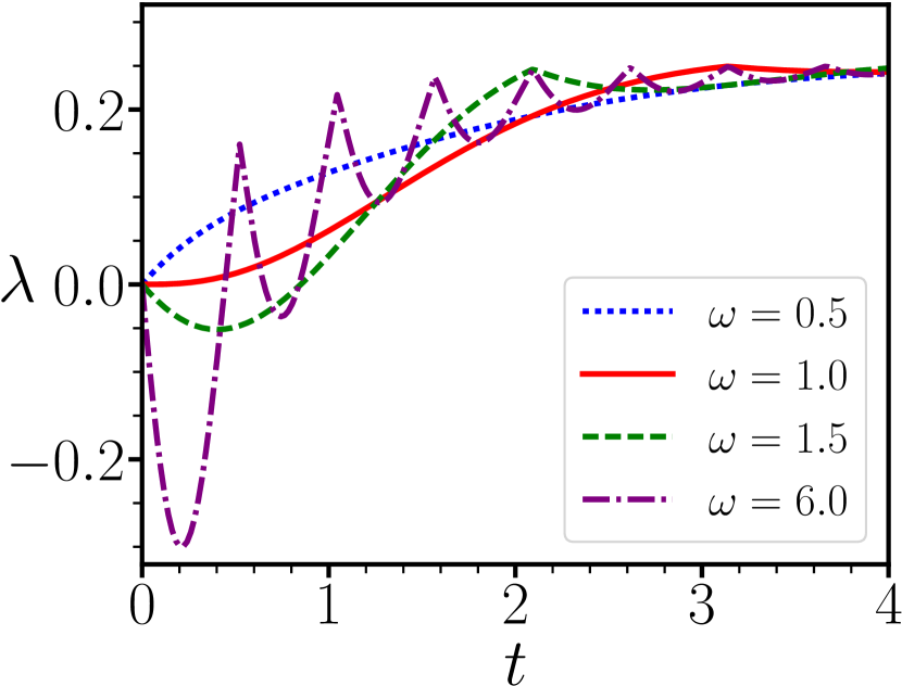
(b)

Figure 2: (a) The smallest eigenvalue $\lambda$ of the partial transposition of $\rho$ as a function of time. (b) The optimal time where the two particles are most entangled. The dashed-line indicates the asymptotic optimal time in the limit of very strong couplings $\omega$ and no decoherence, given by $\pi/(2\omega)$.

III Stochastic fluctuations in preparing the experiment

Let us consider now the fluctuations of the parameters of the experiment. If the separation between the two positions of a particle $L$ is large in comparison to the typical wave length of the electromagnetic environment, we can assume that the decoherence time $T$ is not sensitive to this separation Schlosshauer (2007). Moreover, if $L$ is much larger than $d$, fluctuations in $L$ have only marginal effects on $\Delta$. Thus, only fluctuations in two quantities are important: (a) fluctuations in the minimal distance between the two particles $d$, which induce fluctuations in the coupling $\omega$ and (b) fluctuations in the interaction duration $t$.

To model the fluctuations, one can simply replace the deterministic values of $\omega$ and $t$ by two gaussian random variables $\omega+\xi_{\omega}s_{\omega}$ and $t+\xi_{t}s_{t}$, where $s_{\omega}$ and $s_{t}$ are their standard deviations, and $\xi_{\omega}$ and $\xi_{t}$ are two standard gaussian random variables. The state of the system averaged over all runs of the experiment would then be

$$\bar{\rho}=\langle\rho(t)\rangle_{\xi_{t},\xi_{\omega}}.$$ (11)

Assuming that the fluctuations are small, $t\gg s_{t}$, $\omega\gg s_{\omega}$, one can expand their contributions in the phase and the damping terms in $\rho$ to the first order in $s_{\omega}$ and $s_{t}$. Averaging over the gaussian fluctuations in time $t$ and in coupling parameter $\omega$ then yields the state

$$\bar{\rho}=\frac{1}{4}\begin{pmatrix}1&a&a&b\\ \bar{a}&1&b&\bar{a}\\ \bar{a}&b&1&\bar{a}\\ b&a&a&1\end{pmatrix},$$ (12)

with $a=e^{i\omega t-t}e^{-\frac{1}{2}s_{\omega}^{2}t^{2}+\frac{1}{2}s_{t}^{2}(i\omega-1)^{2}}$ and $b=e^{-2t}e^{2s_{t}^{2}}$.

To analyse the entanglement in the density operator, we again compute the smallest eigenvalue $\bar{\lambda}$ of the partial transposition of $\bar{\rho}$, which is

$$\frac{1}{2}e^{-(t-s_{t}^{2})}[\operatorname{sh}(t-s_{t}^{2})-e^{-\frac{s_{t}^{2}}{2}(1+\omega^{2})-\frac{s_{\omega}^{2}}{2}t^{2}}|\sin\omega(t-s_{t}^{2})|].$$ (13)

By sending $s_{\omega}$ and $s_{t}$ to zero, we can easily recover equation (9). Note that one should not extrapolate this formula to $t<s_{t}^{2}$, since in this regime the fluctuations in time extrapolate the decoherence dynamics backward into negative time, which is not physical. One then finds that the entanglement between the particles develops after $t>s_{t}^{2}$ if and only if

$$s_{t}^{2}(1+s_{t}^{2}s_{\omega}^{2}+\omega^{2})<2\ln\omega.$$ (14)

To be consistent with the approximation, the higher order term $s_{t}^{2}s_{\omega}^{2}$ should in fact be ignored. We thus obtain the condition

$$s_{t}^{2}<\frac{2\ln\omega}{1+\omega^{2}}.$$ (15)

Remarkably, $s_{\omega}$ is absent in this condition. This means that if $\omega>1$, and if the duration of interaction is well-controlled ($s_{t}\approx 0$), the entanglement persists despite arbitrary fluctuations in $\omega$. On the other hand, equation (15) does pose a bound on the maximal standard deviation $s_{t}$ allowed, which is plotted in Figure 3. Interestingly, this indicates that if the interaction strength is strong, one has to control the time more accurately; on the other hand, in the intermediate regime, $s_{t}$ can vary to a large extent. If the interaction time can be precisely controlled by an atomic clock, this accuracy can be easily achieved. In reality, the accuracy of the interaction duraction in the actual experiment could be much less than the scale of atomic clocks due to various difficulties in setting up the superposition configuration for each particle. In particular, it is known Baym and Ozawa (2008); Mari et al. (2016); Belenchia et al. (2018) that such a process should not be too fast, otherwise gravitational radiations would interfere with the system causing further decoherence effects. Yet, we expect that even in this case condition (15) can be easily achieved in reality.

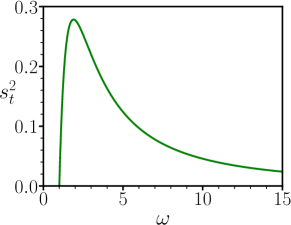
Figure 3: Maximum fluctuation allowed in the interaction duration $s_{t}^{2}$ such that the entanglement can still be observed as a function of the coupling strength $\omega$.

IV Violation of the CHSH inequality

While the entanglement in the density operator can be demonstrated by state tomography or certain entanglement witnesses Gühne and Tóth (2009), it is generally desirable to demonstrate the entanglement in a device-independent way Brunner et al. (2014). This can be done by demonstrating a violation of the so-called Clauser-Horne-Shimony-Holt (CHSH) inequality Brunner et al. (2014). Suppose two parties, Alice and Bob, each of whom owns one particle of the pair. Consider a situation where Alice performs either one of two measurements $A_{1},A_{2}$ on her particle while Bob performs either measurements $B_{1}$ or $B_{2}$ on his particle. Each measurement has only two outcomes $\pm 1$. If one constrains that the system satifies the so-called assumption of local realism Einstein et al. (1935); Bell (1964), then it is easy to show that

$$\left|\langle A_{1}B_{1}\rangle+\langle A_{1}B_{2}\rangle+\langle A_{2}B_{1}\rangle-\langle A_{2}B_{2}\rangle\right|\leq 2.$$ (16)

It has been repeatedly demonstrated in experiments that the CHSH inequality is violated in quantum mechanics Brunner et al. (2014). This shows that quantum mechanics is not compatible with the assumption of local realism, on which the CHSH inequality (16) is based. What is relevant to us in the current context is that in order to violate the CHSH inequality (16) the state must be entangled. Notice that in order to demonstrate the violation of the CHSH inequality, we only need the statistics of the measurements $A_{1},A_{2}$ and $B_{1},B_{2}$ in the experiment. The details how such measurements are setup or how they are described mathematically are irrelevant Brunner et al. (2014). In that sense, one can prove entanglement between particles in a device-independent way.

For simplicity we ignore the fluctuations in the experimental parameters in this section so that the density operator is of the simple form as in equation (8). To see whether $\rho$ violates the CHSH inequality for certain measurement settings, we make use of the criterion described in Ref. Horodecki et al. (1995). To this end, we consider the correlation matrix $T_{ij}=\operatorname{Tr}[\rho\sigma_{i}\otimes\sigma_{j}]$, where $\sigma_{i}$ and $\sigma_{j}$ for $1\leq i,j\leq 3$ are the Pauli matrices. It turns out that the correlation matrix $T$ for $\rho$ is degenerate with singular values $s_{1}=e^{-2t}$ and $s_{2}=s_{3}=e^{-t}\left|\sin\omega t\right|$. Then according to Horodecki et al. (1995), the state $\rho$ violates the CHSH inequality if and only if either $s_{1}^{2}+s_{2}^{2}>1$ or $2s_{2}^{2}>1$. Solving these two inequalities numerically, we find that the system can violate the CHSH inequality if and only if

$$\omega>4.19135.$$ (17)

While this bound is significantly larger than the threshold of the coupling for the systems to be entangled over time ($\omega>1$), it is still in the same order of magnitude. Thus once one can prove the entanglement of the particles, one is also close to proving it in a device-independent manner.

V Conclusion

In this work we have analysed the entanglement dynamics of the two particles in the BMV experiment in detail. We showed that the system entangles as long as the coupling between the particles is strong, $\Delta T/\hbar>1$, and the parameters are setup precisely. Fluctuations in the parameters that arise from setting up the experiment from run to run were then considered. The entanglement turns out robust against the decoherence for some time and also against stochastic fluctuations. Moreover, we discuss the optimal duration of the gravitational interaction while the particles are in a superposition state. Also, we identify a condition under which one can detect entanglement in a device-independent manner using the CHSH inequality. We would like to mention that recently a similar detailed analysis of the entanglement dynamics has been made for another setup of the experiment Kristanda et al. (2019). We hope that together these analyses provide useful inputs for a realisation of the experiment in the near future.