KMT-2018-BLG-0029Lb: A Very Low Mass-Ratio Spitzer Microlens Planet

1 Introduction

For most microlensing planets, the planet-host mass ratio $q$ is well determined, but the mass of the host, which is generally too faint to be reliably detected, remains unknown. Hence the planet mass also remains unknown. One way to carry out statistical studies in the face of this difficulty is to focus attention on the mass ratios themselves. Suzuki et al. (2016) conducted such a study, finding a break in the mass-ratio function at $q_{\rm br}\sim 1.7\times 10^{-4}$ based on planets detected in the MOA-II survey. Udalski et al. (2018) applied a $V/V_{\rm max}$ technique to the seven then-known microlensing planets with well measured $q<10^{-4}$ and confirmed that the slope of the mass-ratio function declines with decreasing mass ratio in this regime. Jung et al. (2019a) considered all planets with $q<3\times 10^{-4}$ and concluded that if the mass-ratio function is treated as a broken power law, then the break is at $q_{\rm br}\simeq 0.56\times 10^{-4}$, with a change in the power-law index of $\zeta>1.6$ at $2\,\sigma$. However, they also noted that there were no detected microlensing planets with $q<0.5\times 10^{-4}$ and suggested that the low end of the mass-ratio function might be better characterized by a “pile-up” around $q\sim 0.7\times 10^{-4}$ rather than a power-law break.

In principle, one might worry that the paucity of detected microlensing planets for $q{\lesssim}0.5\times 10^{-4}$ could be due to poor sensitivity at these mass ratios, which might then be overestimated in statistical studies. However, the detailed examination by Udalski et al. (2018) showed that several planetary events would have been detected even with much lower mass ratios. In particular, they showed that OGLE-2017-BLG-1434Lb would have been detected down to $q=0.018\times 10^{-4}$ and that OGLE-2005-BLG-169Lb would have been detected down to $q=0.063\times 10^{-4}$. Hence, the lack of detected planets $q{\lesssim}0.5\times 10^{-4}$ remains a puzzle.

A substantial subset of microlensing planets, albeit a minority, do have host-mass determinations. For most of these the mass is determined by combining measurements of the Einstein radius $\theta_{\rm E}$ and the microlens parallax ${\mbox{\boldmath$\pi$}}_{\rm E}$ (Gould, 1992, 2000),

$$M={\theta_{\rm E}\over\kappa\pi_{\rm E}};\quad\pi_{\rm rel}=\theta_{\rm E}\pi_{\rm E};\quad\kappa\equiv{4G\over c^{2}{\rm AU}}\simeq 8.1\,{{\rm mas}\over M_{\odot}},$$ (1)

where

$$\theta_{\rm E}=\sqrt{\kappa M\pi_{\rm rel}};\qquad{\mbox{\boldmath$\pi$}}_{\rm E}={\pi_{\rm rel}\over\theta_{\rm E}}\,{{\mbox{\boldmath$\mu$}}_{\rm rel}\over\mu_{\rm rel}},$$ (2)

and $\pi_{\rm rel}$ and ${\mbox{\boldmath$\mu$}}_{\rm rel}$ are the lens-source relative parallax and proper motion, respectively. While $\theta_{\rm E}$ is routinely measured for caustic-crossing planetary events (the great majority of those published to date), ${\mbox{\boldmath$\pi$}}_{\rm E}$ usually requires significant light-curve distortions induced by deviations from rectilinear lens-source relative motion caused by Earth’s annual motion. Thus, either the event must be unusually long or the parallax parameter $\pi_{\rm E}=\sqrt{\pi_{\rm rel}/\kappa M}$ must be unusually big. These criteria generally bias the sample to nearby lenses, e.g., MOA-2009-BLG-266Lb (Muraki et al., 2011), with lens distance $D_{L}\simeq 3\,{\rm kpc}$, which was the first microlens planet with a clear parallax measurement. In a few cases, the host mass has been measured by direct detection of its light (Bennett et al., 2006, 2015; Batista et al., 2014, 2015), but see also Bhattacharya et al. (2017). This approach is also somewhat biased toward nearby lenses, although the main issue is that the lenses are typically much fainter than the sources, in which case one must wait many years for the two to separate sufficiently on the plane of the sky to make useful observations.

Space-based microlens parallaxes (Refsdal, 1966; Gould, 1994; Dong et al., 2007) provide a powerful alternative, which is far less biased toward nearby lenses. Since 2014, Spitzer has observed almost 800 microlensing events toward the Galactic bulge (Gould et al., 2013, 2014, 2015a, 2015b, 2016) with the principal aim of measuring the Galactic distribution of planets. In order to construct a valid statistical sample, Yee et al. (2015) established detailed protocols that govern the selection and observational cadence of these microlensing targets.

For 2014–2018, the overwhelming majority of targets were provided by the Optical Gravitational Lensing Experiment (OGLE, Udalski et al. 2015b) Early Warning System (EWS, Udalski et al. 1994; Udalski 2003), with approximately 6% provided by the Microlensing Observations for Astrophysics (MOA, Bond et al. 2004) collaboration. In June 2018, the Korea Microlensing Telescope Network (KMTNet Kim et al. 2016) initiated a pilot alert program, covering about a third of its fields (Kim et al., 2018d). In order to maximize support for Spitzer microlensing, these fields were chosen to be in the northern Galactic bulge, which is relatively disfavored by microlensing surveys due to higher extinction, an effect that hardly impacts Spitzer observations at $3.6\mu$m. This pilot program contributed about 17% of all 2018 Spitzer alerts. None of these events had obvious planetary signatures in the original online pipeline reductions. However, after the re-reduction of all 2018 KMT-discovered events (including those found by the post-season completed-event algorithm, Kim et al. 2018a), one of these Spitzer alerts, KMT-2018-BLG-0029, showed a hint of an anomaly in the light curve. This triggered tender loving care (TLC) re-reductions, which then revealed a clear planetary candidate.

The lens system has the lowest planet-host mass ratio $q=0.18\times 10^{-4}$ of any microlensing planet found to date by more than a factor of two.

2 Observations

2.1 KMT Observations

KMT-2018-BLG-0029 is at (RA,Dec) = (17:37:52.67, $-27$:59:04.92), corresponding to $(l,b)=(-0.09,+1.95)$. It lies in KMT field BLG14, which is observed by KMTNet with a nominal cadence of $\Gamma=1.0\,{\rm hr}^{-1}$ from its three sites at CTIO (KMTC), SAAO (KMTS), and SSO (KMTA) using three identical 1.6m telescopes, each equipped with a $4\,{\rm deg}^{2}$ camera. The nominal cadence is maintained for all three telescopes during the “Spitzer season” (which formally began for 2018 on HJD${}^{\prime}={\rm HJD}-2450000=8294.7$). But prior to this date, the cadence at KMTA and KMTS was at the reduced rate of $\Gamma=0.75\,{\rm hr}^{-1}$. The change to higher cadence fortuitously occurred just a few hours before the start of the KMTA observations of the anomaly.

The event was discovered on 30 May 2018 during “live testing” of the alert-finder algorithm, and was not publicly released until 21 June. However, as part of the test process, this (and all) alerts were made available to the Spitzer team (see Section 2.2, below).

The great majority of observations were carried out in the $I$ band, but every tenth such observation is followed by a $V$-band observation that is made primarily to determine source colors. All reductions for the light curve analysis were conducted using pySIS (Albrow et al., 2009), which is a specific implementation of difference image analysis (DIA, Tomaney, & Crotts 1996; Alard & Lupton 1998).

2.2 Spitzer Observations

The event was chosen by the Spitzer microlensing team at UT 23:21 on 19 June (JD${}^{\prime}=8289.47$). The observational cadence was specified as “priority 1” (observe once per cycle of Spitzer-microlensing time) for the first two weeks and “priority 2” thereafter (all subsequent cycles). Because the target lies well toward the western side of the microlensing fields, it was one of the relatively few events that were within the Spitzer viewing zone during the beginning of the Spitzer season. Therefore, it was observed (5, 4, 2, 2) times on (1, 2, 3, 4) July, compared to roughly one time per day for “priority 1” targets during the main part of the Spitzer season.

We note that the event was chosen by the Spitzer team about five days prior to the anomaly. However, as mentioned in Section 1, the anomaly could not be discerned from the on-line reduction in any case. The planet KMT-2018-BLG-0029Lb will therefore be part of the Spitzer microlensing statistical sample (Yee et al., 2015).

Like almost all other planetary events from the first five years (2014-2018) of the Spitzer microlensing program, KMT-2018-BLG-0029 was reobserved at baseline during the (final) 2019 season in order to test for systematic errors, which were first recognized in Spitzer microlensing data by Zhu et al. (2017). See in particular, their Figure 6. Significant additional motivation for this decision came from the work of Koshimoto & Bennett (2019), who developed a quantitative statistical test that they applied to the Zhu et al. (2017) sample and subsamples. In the case of KMT-2018-BLG-0029, there were 15 epochs over 3.6 days near the beginning of the bulge observing window. This relatively high number (compared to other archival targets) was again due to the fact that KMT-2018-BLG-0029 lies relatively far to the west, so that there were relatively few competing targets during the first week of observations.

The Spitzer data were reduced using customized software that was written for the Spitzer microlensing program (Calchi Novati et al., 2015).

As we discuss in Section 5.1, the latter half of the 2018 Spitzer data suffer from correlated residuals. We investigate this in detail in the Appendix, where we identify the likely cause of these correlated errors. We therefore remove these data from the main analysis and only consider them within the context of the investigation in the Appendix.

2.3 SMARTS ANDICAM Observations

The great majority of Spitzer events, particularly those in regions of relatively high extinction, are targeted for $I/H$ observations using the ANDICAM dual-mode camera (DePoy et al., 2003) mounted on the SMARTS 1.3m telescope at CTIO. The purpose of these observations is to measure the source color, which is needed both to measure the angular radius of the source (Yoo et al., 2004) and to facilitate a color-color constraint on the Spitzer source flux (Yee et al., 2015; Calchi Novati et al., 2015). For this purpose, of order a half-dozen observations are usually made at a range of magnifications. Indeed, five such measurements were made of KMT-2018-BLG-0029. Each $H$-band observation is split into five 50-second dithered exposures.

The 2018 $H$-band observations did not extend to (or even near) baseline in part because the event is long but mainly because of engineering problems at the telescope late in the 2018 season. Hence, these data cover a range of magnification $12{\lesssim}A{\lesssim}33$. We therefore obtained six additional $H$-band epochs very near baseline in 2019. The $H$-band data were reduced using DoPhot (Schechter et al., 1993).

We note that in the approximations that the magnified data uniformly sample the magnification range $A_{\rm low}\leq A\leq A_{\rm high}$ with $n$ points and that the photometric errors are constant in flux (generally appropriate if all the observations are below sky), the addition of $m$ points at baseline $A_{\rm base}=1$ will improve the precision of color measurement by a factor,

$${\sigma_{\rm w/o-base}\over\sigma_{\rm with-base}}=\sqrt{1+K{m\over m+n}};\quad K\equiv 12{n-1\over n+1}\biggl{(}{\delta A\over\Delta A}\biggr{)}^{2},$$ (3)

where $\delta A\equiv[(A_{\rm high}+A_{\rm low})/2-A_{\rm base}]$ and $\Delta A\equiv(A_{\rm high}-A_{\rm low})$. Equation (3) can be derived by explicit evaluation of the more general formula $\sigma({\rm slope})=\sigma_{\rm meas}/\sqrt{n\,{\rm var}(A)}$ (Gould, 2003). Of course, the conditions underlying Equation (3) will never apply exactly, but it can give a good indication of the utility of baseline observations. In our case $K=12(4/6)(21.5/21)^{2}=8.4$, so the predicted improvement was a factor 2.4. The actual improvement was a factor 2.0, mainly due to worse conditions (hence larger errors) at baseline.

3 Ground-Based Light Curve Analysis

3.1 Static Models

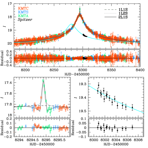
Figure 1: Light curve and best fit model for KMT-2018-BLG-0029. The cusp crossing of the anomaly (lower-left panel) is covered by five points, but the approaches to and from this crossing trace the overall “dip” that typically characterizes transverse cusp approaches. These features are caused by a planet with mass ratio $q=1.8\pm 0.2\times 10^{-5}$, the lowest of any microlensing planet to date by more than a factor two. The Spitzer “$L$-band” data, which are shown in greater detail in the lower-right panel, have been aligned (as usual) to the $I$-band scale by $f_{\rm display}=(f_{L}-f_{b,L})(f_{s,I}/f_{s,L})+f_{b,I}$ (and then converted to magnitudes). Their role in measuring the microlens parallax ${\mbox{\boldmath$\pi$}}_{\rm E}$ is greatly aided by the $IHL$ color-color relation which constrains the ratio in this expression $(f_{s,I}/f_{s,L})=10^{-0.4(I-L)}$ to a few percent. See Section 4.3. Paczyński (1L1S, dashed line) and binary-source (1L2S, dotted line) models are clearly excluded by the data. See Figure 2 for the full Spitzer light curve, which includes 2019 “baseline” data.

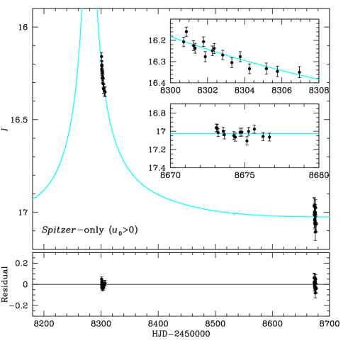
Figure 2: Full Spitzer light curve including the 2018 data (see Figure 1) and the 2019 “baseline” data. Only the first half of the 2018 data (covering the first six days in time) are included in the fit and are shown here. See Section 5.1 and the Appendix for details.

With the exception of five “high points” near the peak of the event, the KMT light curve (Figure 1) looks essentially like a standard single-lens single-source (1L1S) Paczyński (1986) event, which is characterized by three geometric parameters $(t_{0},u_{0},t_{\rm E})$, i.e., the time of lens-source closest approach, the impact parameter of this approach (normalized to $\theta_{\rm E}$), and the Einstein timescale, $t_{\rm E}=\theta_{\rm E}/\mu_{\rm rel}$. The five high points span just 4.4 hours, and they are flanked by points taken about one hour before and after this interval that are qualitatively consistent with the underlying 1L1S curve. However, the neighboring few hours of data on each side of the spike actually reveal a gentle “dip” within which the spike erupts. Hence, the pronounced perturbation is very short, i.e., of order a typical source diameter crossing time $2t_{*}\equiv 2\theta_{*}/\mu_{\rm rel}$, where $\theta_{*}$ is the angular radius of the source. Given that the perturbation takes place at peak, the most likely explanation is that the lens has a companion, for which the binary-lens axis is oriented very nearly at $\alpha=\pm 90^{\circ}$ relative to ${\mbox{\boldmath$\mu$}}_{\rm rel}$. Moreover, the source must be passing over either a cusp or a narrow magnification ridge that extends from a cusp.

Notwithstanding this naive line of reasoning, we conduct a systematic search for binary-lens solutions. We first conduct a grid search over an $(s,q)$ grid, where $s$ is the binary separation in units of $\theta_{\rm E}$ and $q$ is the binary mass ratio. We fit each grid point with a seven-parameter (“standard”) model $(t_{0},u_{0},t_{\rm E},s,q,\alpha,\rho)$, where $(s,q)$ are held fixed and the five other parameters are allowed to vary. The three Paczyński parameters are seeded at their 1L1S values, while $\alpha$ is seeded at six different values drawn uniformly from the unit circle. The last parameter, $\rho\equiv\theta_{*}/\theta_{\rm E}=t_{*}/t_{\rm E}$ is seeded at $\rho=(4.4\,{\rm hr})/2t_{\rm E}\rightarrow 1\times 10^{-3}$ following the argument given above. In addition to these non-linear parameters there are two linear parameters for each observatory, i.e., the source flux $f_{s}$ and the blended flux $f_{b}$. Hence, the observed flux is modeled as $F(t)=f_{s}A(t)+f_{b}$, where $A(t)$ is the time-dependent magnification at a given observatory.

Table 1: Best-fit solutions for ground-only data

		Parallax models
Parameters	Standard	$u_{0}>0$	$u_{0}<0$
$\chi^{2}/\rm{dof}$	1855.231/1852	1849.908/1850	1849.504/1850
$t_{0}$ $(\rm{HJD}^{\prime})$	8294.702 $\pm$ 0.023	8294.709 $\pm$ 0.025	8294.704 $\pm$ 0.027
$u_{0}$	0.028 $\pm$ 0.003	0.026 $\pm$ 0.002	-0.027 $\pm$ 0.002
$t_{\rm E}$ $(\rm{days})$	169.106 $\pm$ 20.595	176.815 $\pm$ 13.742	172.151 $\pm$ 14.743
$s$	1.000 $\pm$ 0.002	0.999 $\pm$ 0.003	1.000 $\pm$ 0.002
$q$ $(10^{-5})$	1.870 $\pm$ 0.243	1.817 $\pm$ 0.267	1.816 $\pm$ 0.215
$\alpha$ $(\rm{rad})$	1.529 $\pm$ 0.005	1.529 $\pm$ 0.005	-1.529 $\pm$ 0.006
$\rho$ $(10^{-4})$	4.603 $\pm$ 0.772	4.414 $\pm$ 0.683	4.577 $\pm$ 0.693
$\pi_{\rm{E},\it{N}}$	-	-0.111 $\pm$ 0.084	-0.266 $\pm$ 0.149
$\pi_{\rm{E},\it{E}}$	-	0.103 $\pm$ 0.045	0.089 $\pm$ 0.035
$\pi_{\rm{E}}$	-	0.151 $\pm$ 0.080	0.280 $\pm$ 0.126
$\phi_{\pi}$	-	2.391 $\pm$ 0.570	2.819 $\pm$ 0.673
$f_{S}({\rm CTIO})$	0.029 $\pm$ 0.003	0.028 $\pm$ 0.003	0.029 $\pm$ 0.003
$f_{B}({\rm CTIO})$	0.123 $\pm$ 0.001	0.129 $\pm$ 0.003	0.129 $\pm$ 0.003
$t_{*}$ $(\rm{days})$	0.078 $\pm$ 0.009	0.078 $\pm$ 0.009	0.079 $\pm$ 0.009

Notes, $\pi_{\rm E}\equiv\sqrt{\pi_{{\rm E},N}^{2}+\pi_{{\rm E},E}^{2}}$, $\phi_{\pi}\equiv\tan^{-1}(\pi_{{\rm E},E}/\pi_{{\rm E},N})$, and $t_{*}\equiv\rho t_{\rm E}$ are derived quantities and are not fitted independently. All fluxes are on an 18th magnitude scale, e.g., $I_{s}=18-2.5\,\log(f_{s})$.

This grid search yields only one local minimum, which we refine by allowing all seven parameters to vary during the $\chi^{2}$ minimization. See Figure 1 and Table 1. Note that for compactness of exposition, Figure 1 shows the Spitzer data in addition to the ground-based data. However, here (in Section 3) we are considering results from the ground-based data alone. See Figure 2 for the full, 2018-2019 Spitzer light curve. As anticipated, the binary axis is perpendicular to ${\mbox{\boldmath$\mu$}}_{\rm rel}$. See Figure 3 for the caustic geometry.

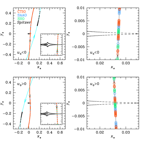
Figure 3: Caustic geometries for the two parallax solutions ($u_{0}>0$ and $u_{0}<0$). The insets show the times of the ground-based observations, color-coded by observatory, with the source size shown to scale. The right panels are zooms of these insets.

3.2 Binary Source Model

In principle, the short-lived “bumps” induced on the light curve by planets (such as the one in Figure 1) can be mimicked by configurations in which there are two sources (1L2S) instead of two lenses (2L1S) (Gaudi, 1998). Hence, unless there are obvious caustic features, one should always check for 1L2S solutions. In the present case, while there are caustic features, they are less than “completely obvious”.

Relative to 1L1S (Paczyński, 1986) models, the 1L2S model has four additional parameters: the $(t_{0},u_{0})_{2}$ peak parameters of the second source, $\rho_{2}$, i.e., the radius ratio of the second source to $\theta_{\rm E}$, and $q_{F,I}$, the $I$-band flux ratio of the second source to the first.

Figure 1 shows the best-fit 1L2S model, and Table 2 shows the best-fit parameters. For completeness, this table also shows the best fit 1L1S model. The 1L2S model has $\Delta\chi^{2}=130$ relative to the standard 2L1S model. Moreover, it does not qualitatively match the features of the light curve, as shown in Figure 1. Therefore, we exclude 1L2S models.

Table 2: Best-fit solutions for 1L1S and 1L2S models

Parameters	1L1S	1L2S
$\chi^{2}/\rm{dof}$	2544.293/1856	1985.237/1852
$t_{0,1}$ $(\rm{HJD}^{\prime})$	8294.715 $\pm$ 0.022	8294.639 $\pm$ 0.025
$u_{0,1}$	0.026 $\pm$ 0.003	0.031 $\pm$ 0.003
$t_{\rm E}$ $(\rm{days})$	179.591 $\pm$ 17.963	156.531 $\pm$ 12.943
$t_{0,2}$ $(\rm{HJD}^{\prime})$	-	8294.908 $\pm$ 0.002
$u_{0,2}$ $(10^{-5})$	-	1.101 $\pm$ 3.348
$\rho_{2}$ $(10^{-4})$	-	1.305 $\pm$ 0.785
$qF,I$ $(10^{-3})$	-	1.851 $\pm$ 0.187
$f_{S}$	0.028 $\pm$ 0.003	0.032 $\pm$ 0.003
$f_{B}$	0.125 $\pm$ 0.001	0.122 $\pm$ 0.001

3.3 Ground-Based Parallax

Because the event is quite long, $t_{\rm E}>100\,$day, the ground-based light curve alone is likely to put significant constraints on the microlens parallax ${\mbox{\boldmath$\pi$}}_{\rm E}$. It is important to evaluate these constraints in order to compare them with those obtained from the Spitzer light curve, as a check against possible systematics in either data set. We therefore begin by fitting for parallax from the ground-based light curve alone, introducing two additional parameters $(\pi_{{\rm E},N},\pi_{{\rm E},E})$, i.e., the components of ${\mbox{\boldmath$\pi$}}_{\rm E}$ in equatorial coordinates.

We also introduce two parameters for linearized orbital motion ${\mbox{\boldmath$\gamma$}}\equiv((ds/dt)/s,d\alpha/dt)$ because these can be correlated with ${\mbox{\boldmath$\pi$}}_{\rm E}$ (Batista et al., 2011; Skowron et al., 2011). Here $ds/dt$ is the instantaneous rate of change of $s$, and $d\alpha/dt$ is the instantaneous rate of change of $\alpha$, both evaluated at $t_{0}$. We expect (and then confirm) that $\gamma$ may be relatively poorly constrained and so range to unphysical values. We therefore limit the search to $\beta<0.8$, where $\beta$ is the ratio of projected kinetic to potential energy (Dong et al., 2009),

$$\beta\equiv\bigg{|}{\rm KE_{\perp}\over PE_{\perp}}\bigg{|}={\kappa M_{\odot}(\rm yr)^{2}\over 8\pi^{2}}{\pi_{\rm E}\over\theta_{\rm E}}\gamma^{2}\biggl{(}{s\over\pi_{\rm E}+\pi_{s}/\theta_{\rm E}}\biggr{)}^{3},$$ (4)

and where we adopt $\theta_{*}=0.70\,{\mu\rm as}$ from Section 4.2 (and thus, $\theta_{\rm E}=\theta_{*}/\rho$) and $\pi_{s}=0.12$ for the source parallax. We note that while bound orbits strictly obey $\beta<1$, we set the limit slightly lower because of the extreme paucity of highly eccentric planets, and the very low probability of observing them at a phase and orientation such that $\beta>0.8$. We find that with $\beta$ (and thus $\gamma$) so restricted, $\gamma$ is neither significantly constrained nor strongly correlated with ${\mbox{\boldmath$\pi$}}_{\rm E}$. Hence, we eliminate it from the fit.

As usual, we check for a degenerate solution with $u_{0}\rightarrow-u_{0}$ (Smith et al., 2003), which is often called the “ecliptic degeneracy” because it is exact to all orders on the ecliptic (Jiang et al., 2005), and which can be extended to binary and higher-order parameters (Skowron et al., 2011). Indeed, we find a nearly perfect degeneracy. See Table 1.

Before incorporating the Spitzer data we must first investigate the color properties of the source.

4 Color-Magnitude Diagram (CMD)

The source color and magnitude are important for two reasons. First, they enable a measurement of $\theta_{*}$, and so of $\theta_{\rm E}=\theta_{*}/\rho$ (Yoo et al., 2004). Second, one can combine the source color with a color-color relation to derive a constraint on the Spitzer source flux (Yee et al., 2015; Calchi Novati et al., 2015). Table 3 lists many photometric properties of the source.

Table 3: Derived Photometric Properties of Source

Quantity	mag
$A_{I}$	$3.39$
$I_{s,\rm pydia}$	$22.02\pm 0.08$
$I_{s,\rm stand}$	$21.84\pm 0.12$
$H_{s}$	$18.24\pm 0.08$
$(I_{\rm pydia}-H)_{s}$	$3.78\pm 0.02$
$(I-H)_{0,s}$	$0.87\pm 0.03$
$(V-I)_{0,s}$	$0.78\pm 0.03$
$(V-K)_{0,s}$	$1.71\pm 0.07$

Note, Instrumental $I_{\rm pydia}$ is calibrated to standard $I$ from the tabulated extinction and the known position of the clump. $H$-band data are on VVV system.

4.1 Source Position on the CMD

The source is heavily extincted, $A_{I}\simeq 3.39$ (Gonzalez et al. 2012, where we adopt $A_{I}=7\,A_{K}$ from a regression of $A_{I}$ from Nataf et al. 2013 on $A_{K}$ from Gonzalez et al. 2012). Therefore, the $V$-band data that are routinely taken by KMT are too noisy to measure a reliable source color. However, as discussed in Section 2, KMT-2018-BLG-0029 (similar to most Spitzer targets) was observed at five epochs in $H$ band and then was additionally observed at six epochs near baseline.

We can therefore place the source on an instrumental $(I-H,I)$ CMD by combining these observations with the $I$-band observations from KMTC, which is located at the same site as the SMARTS telescopes. To do so, we first reduce the KMTC light curve and photometer the stars within a $2^{\prime}\times 2^{\prime}$ square on the same instrumental system using pyDIA. We then evaluate the $(I-H)$ instrumental color by regression, finding $(I_{\rm pyDIA}-H_{\rm ANDICAM})=-1.035\pm 0.019$. In order to apply the method of Yoo et al. (2004) we must compare this color to that of the red giant clump. However, the ANDICAM data do not go deep enough to reliably trace the clump. We therefore align the ANDICAM system to the VVV survey (Minniti et al., 2017), finding $(H_{\rm ANDICAM}-H_{\rm VVV})=4.817\pm 0.005$ and therefore $(I_{\rm pyDIA}-H_{\rm VVV})=3.782\pm 0.019$. We then find $I_{\rm pyDIA}=22.02\pm 0.02$ by fitting the pyDIA light curve to the best model from Section 3.3. We form an $(I-H,I)$ CMD by cross-matching the KMTC-pyDIA and VVV field stars. Figure 4 shows the source position on this CMD.

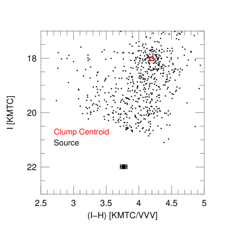
Figure 4: Color-magnitude diagram (CMD) for stars within a $2^{\prime}$ square centered on KMT-2018-BLG-0029. The $I$-band data come from pyDIA reductions of KMTC data while the $H$-band data come from the VVV catalog. The source $I$ magnitude (black) derives from the fit to the light curve while the source $(I-H)$ color comes from regression of the SMARTS ANDICAM $H$-band light curve (aligned to the VVV system) on the $I$-band light curve. The red giant clump centroid is shown in red.

4.2 $\theta_{\rm E}$ and $\mu_{\rm rel}$

We next measure the clump centroid on this CMD, finding $[(I-H),I]_{\rm clump}=(4.20,18.02)\pm(0.02,0.04)$, which then yields an offset from the clump of $\Delta[(I-H),I]=(-0.42,3.98)\pm(0.02,0.03)$. We adopt $[(V-I),I]_{0,\rm clump}=(1.06,14.45)$ from Bensby et al. (2013) and (Nataf et al., 2013), and use the color-color relations of Bessell & Brett (1988), to derive $(V-K,V)_{0}=(1.71,19.21)$. That is, the source is a late G star that is very likely on the turnoff/subgiant branch. Applying the color/surface-brightness relation of Kervella et al. (2004), we find,

$$\theta_{*}=0.70\pm 0.05\,{\mu\rm as}.$$ (5)

Combining Equation (5) with $\rho$ and $t_{\rm E}$ from the ground-based parallax solutions in Table 1, this implies,

$$\theta_{\rm E}={\theta_{*}\over\rho}=1.56\pm 0.24\,{\rm mas};\quad\mu_{\rm rel}={\theta_{\rm E}\over t_{\rm E}}=3.3\pm 0.5\,{{\rm mas}\over\rm yr}.$$ (6)

These values strongly favor a disk lens, $D_{L}{\lesssim}4\,{\rm kpc}$, because otherwise the lens would be massive (thus bright) enough to exceed the observed blended light. However, we defer discussion of the nature of the lens until after incorporating the Spitzer parallax measurement into the analysis.

4.3 IHL Color-Color Relation

We match field star photometry from KMTC-pyDIA ($I$) and VVV $(H)$ (Section 4.1) with Spitzer $(L)$ photometry within the range $3.6<(I-H)<4.5$, to obtain an $IHL$ color-color relation

$$I_{\rm pyDIA}-L=1.18[(I_{\rm pyDIA}-H)_{s}-3.7]+3.32\rightarrow 3.417\pm 0.022,$$ (7)

where the instrumental Spitzer fluxes are converted to magnitudes on an 18th mag system. In order to relate Equation (7) to the pySIS magnitudes reported in this paper (e.g., in Tables 1 and 5), we take account of the offset between these two systems (measured very precisely from regression) $I_{\rm pySIS}-I_{\rm pyDIA}=-0.120\pm 0.005$ to obtain

$$I_{\rm pySIS}-L=3.297\pm 0.022,$$ (8)

We employ this relation when we incorporate Spitzer data in Section 5.

5 Parallax Analysis Including Spitzer Data

5.1 Removal of Second-Half-2018 Spitzer Data

As described in detail in the Appendix, we find that the second half of the 2018 Spitzer KMT-2018-BLG-0029 light-curve shows correlated residuals, and that several nearby stars display similar or related effects. We therefore remove these epochs from the analysis. That is, we include only the first six days of 2018 data as well as all of the 2019 data, which in fact were also taken during the first week (actually first 3.6 days) of the 2019 Spitzer observing window. We very briefly describe the essential elements here but refer the reader to the Appendix for a thorough discussion.

When all data are included in the analysis, there are correlated residuals during 2018, primarily after the first week. That is, the light curve appears “too bright” during this period relative to any model that fits the rest of the data. There are three bright stars within 2 Spitzer pixels, whose combined flux is about 180 times that of the source (i.e., $f_{s,{\it Spitzer}}$). One of these three shows a similar flux offset and another shows anomalously larger scatter during the same period (i.e., after the first week), but all three show essentially identical behavior between the first week of 2018 and the first week of 2019.

All of these empirical characteristics may be explained as due to rotation of the camera during the observations. As part of normal Spitzer operations, the camera orientation rotated at an approximately constant rate of 0.068 deg/day, i.e., by $2.5^{\circ}$ over the whole set of 2018 observations but only by $0.41^{\circ}$ during the first six days. The mean position angle during this six-day period differed from the mean for 2019 by just $0.14^{\circ}$, i.e., 6% of the full rotation during 2018. The pixel response function (PRF, Calchi Novati et al. 2015) photometry should in principle take account of the changing pixel response as a function of camera orientation, but if there are slight errors in the positions of the blends due to severe crowding, then the PRF results will suffer accordingly. Hence, it is plausible that the observed deviations in both the target and blended stars, which are of order 1% of the total flux of the blends, are caused by this rotation. Moreover, there can be other effects of rotation such as different amounts of light from distant stars falling into the grid of pixels being analyzed at each epoch (Calchi Novati et al., 2015). Finally, we note that when the data are restricted to the first six days of 2018 (and first 3.6 days of 2019), the scatter about the model light curve is consistent with the photon-noise-based photometric errors.

5.2 Spitzer-“Only” Parallax

Table 4: Spitzer-“only” models

Parameters	$(u_{0}>0)$	$(u_{0}<0)$
$\chi^{2}/\rm{dof}$	26.000/26	26.217/26
$\pi_{\rm{E},\it{N}}$	-0.023 $\pm$ 0.037	0.024 $\pm$ 0.037
$\pi_{\rm{E},\it{E}}$	0.112 $\pm$ 0.008	0.115 $\pm$ 0.007
$\pi_{\rm{E}}$	0.115 $\pm$ 0.007	0.117 $\pm$ 0.008
$\phi_{\pi}$	1.768 $\pm$ 0.333	1.366 $\pm$ 0.319
$f_{S}(Spitzer)$	0.575 $\pm$ 0.013	0.599 $\pm$ 0.013
$f_{B}(Spitzer)$	1.871 $\pm$ 0.030	1.845 $\pm$ 0.031

Note, $\pi_{\rm E}$ and $\phi_{\pi}$ are derived quantities and are not fitted independently. All fluxes are on an 18th magnitude scale, e.g., $L_{s,Spitzer}=18-2.5\,\log(f_{s,Spitzer})$.

As discussed in Section 3.3, it is important to compare the parallax information coming from the ground and Spitzer separately before combining them, in order to test for systematics. This remains so even though we have located and removed an important source of systematics just above. To trace the information coming from Spitzer, we first suppress the parallax information coming from the ground-based light curve by representing it by its seven non-parallax parameters $(t_{0},u_{0},t_{\rm E},s,q,\alpha,\rho)_{\oplus}$ along with the $I$-band source flux $f_{s,\oplus}$, as taken from Table 1. For this purpose, we use these eight non-parallax parameters taken from the parallax solutions. In this sense, there is some indirect “parallax information” coming from the ground-based fit. However, because we are testing for consistency, we must do this to avoid injecting inconsistent information. (In any case, the standard-model and parallax-model parameters are actually quite similar.)  We apply this procedure separately for the two “ecliptic degeneracy” parallax solutions shown in Table 1.

Figure 5: Likelihood contours $-2\Delta\ln L<(1,4,9)$ for (black, red, yellow) for the parallax vector ${\mbox{\boldmath$\pi$}}_{\rm E}$ in polar coordinates. Green indicates $-2\Delta\ln L>9$. Although the polar-angle $\phi_{\pi}$ distribution is relatively broad for the Spitzer-“only” fits (left panels), the amplitude $\pi_{\rm E}$ is nearly constant because the Spitzer observations are reasonably close to the Gould & Yee (2012) “cheap parallax” limit. See Section 5.3. When “one-dimensional” parallax information from the ground is added (right panels), the amplitude $\pi_{\rm E}$ does not qualitatively change. See also Figures 6 and 7.

The left-hand panels of Figure 5 show likelihood contours in polar coordinates for the $u_{0}>0$ and $u_{0}<0$ solutions of the Spitzer-“only” analysis. See also Table 4. That is, $\pi_{\rm E}=|{\mbox{\boldmath$\pi$}}_{\rm E}|$ is the amplitude and $\phi_{\pi}=\tan^{-1}(\pi_{{\rm E},E}/\pi_{{\rm E},N})$ is the polar angle. For both signs of $u_{0}$, the amplitude $\pi_{\rm E}$ is nearly constant over a broad range of angles. This can be understood within the context of the argument of Gould & Yee (2012), which was then empirically verified by Shin et al. (2018). In the original argument, a single satellite measurement at the epoch of the ground-based peak, $t_{0,\oplus}$, of a high-magnification event (together with a baseline measurement) would yield an excellent measurement of $\pi_{\rm E}$ but essentially zero information about $\phi_{\pi}$. Because the first Spitzer point is six days after $t_{0,\oplus}$, this condition does not strictly hold. However, the mathematical basis of the argument is in essence that $u_{\rm sat}\gg u_{\oplus}$ at the time of this “single observation”. This is reasonably well satisfied for the first Spitzer observation. At this time $u_{\oplus}\sim 0.044$. On the other hand, $A(t)_{\rm spitzer}=1+(F(t)-F_{\rm base})/F_{s}\rightarrow 5.0$ for the first epoch. Thus, $u_{Spitzer}\sim 0.203$. If this had truly been a single-epoch measurement, then the parallax contour would have been an “offset circle” (compared to the well-centered circle of Figure 3 of Shin et al. 2018), with extreme parallax values $\pi_{{\rm E},\pm}=({\rm AU}/D_{\perp})(0.203\pm 0.044)$, i.e., a factor 1.55 difference. Here $D_{\perp}\sim 1.3\,{\rm AU}$ is the projected Earth-Spitzer separation at the measurement epoch. However, the rest of the Spitzer light curve then restricts this circle to an arc. See Figures 1 and 2 of Gould (2019), which also illustrate how the two Spitzer-“only” solutions (for a given sign of $u_{0}\equiv u_{0,\oplus}$) merge. Figure 6 shows the ${\mbox{\boldmath$\pi$}}_{\rm E}$ contours in Cartesian coordinates for the six cases. Here we focus attention on four of these cases, (ground-only, Spitzer-“only”)$\times(u_{0}<0,\ u_{0}>0)$.

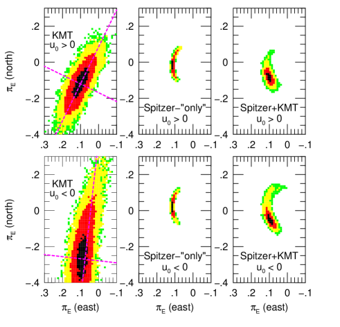
Figure 6: 6-panel diagram of $(\pi_{{\rm E},N},\pi_{{\rm E},E})$ Cartesian contours. The upper panels show the $u_{0}>0$ solutions, while the lower panels show the $u_{0}<0$ solutions. From left to right, we display ground-only, Spitzer-“only”, and combined parallaxes. Black, red, and yellow indicate relative likelihoods $-2\Delta\ln L<$ 1, 4, 9 respectively. Green represents $-2\Delta\ln L>9$. The ground-only data yield approximately linear, “one-dimensional” constraints (Gould et al., 1994; Smith et al., 2003). The Spitzer-“only” data yield an arc opening to the west (direction of Spitzer) because they begin post-peak and are falling rapidly (Gould, 2019). However, the arc is confined to an arclet of relatively constant $\pi_{\rm E}$ amplitude (see Figure 5) because the Spitzer observations begin when the ground data are still highly magnified. For at least one case ($u>0$) the left and center panels are consistent, implying that there is no evidence for systematics. Hence, the two data sets can be combined (right). The magenta lines in the left panels show the principal axes defined by the $2\,\sigma$ contour. For $u_{0}>0$, the contours are nearly elliptical and the minor axis $\psi_{\rm short}=-116^{\circ}$ is almost perfectly aligned to the direction of the Sun at peak: $-117^{\circ}$, both of which reflect “ideal” 1-D parallaxes. For $u_{0}<0$, the ellipse deviates from both conditions.

These show that the ground-only and Spitzer-“only” parallax contours are consistent for the $u>0$ case and marginally inconsistent for the $u<0$ case. The levels of consistency can be more precisely gauged from Figure 7, which shows overlapping contours. Because one of these two cases is consistent, there is no evidence for systematics in either data set. That is, only one of the two cases can be physically correct, so only if both were inconsistent would the comparison provide evidence of systematics.

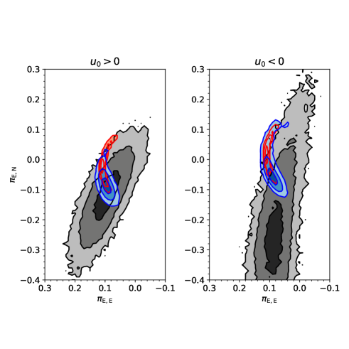
Figure 7: Overlap of three sets of contours shown in Figure 6 for each of the two parallax solutions. This makes it easier to see that for $u_{0}>0$ the ground-only and Spitzer-“only” solutions are consistent, showing that there is no evidence for systematics. Then, the fact that these solutions show some tension for $u_{0}<0$ implies that this solution is somewhat disfavored.

5.3 Full Parallax Models

Table 5: Best-fit solutions for ground+Spitzer data

	Parallax models
Parameters	$u_{0}>0$	$u_{0}<0$
$\chi^{2}/\rm{dof}$	1877.274/1878	1881.580/1878
$t_{0}$ $(\rm{HJD}^{\prime})$	8294.716 $\pm$ 0.025	8294.727 $\pm$ 0.025
$u_{0}$	0.027 $\pm$ 0.003	-0.027 $\pm$ 0.003
$t_{\rm E}$ $(\rm{days})$	173.950 $\pm$ 15.754	176.564 $\pm$ 16.346
$s$	1.000 $\pm$ 0.002	1.000 $\pm$ 0.002
$q$ $(10^{-5})$	1.829 $\pm$ 0.217	1.758 $\pm$ 0.222
$\alpha$ $(\rm{rad})$	1.531 $\pm$ 0.005	-1.534 $\pm$ 0.005
$\rho$ $(10^{-4})$	4.472 $\pm$ 0.692	4.398 $\pm$ 0.708
$\pi_{\rm{E},\it{N}}$	-0.086 $\pm$ 0.028	-0.054 $\pm$ 0.042
$\pi_{\rm{E},\it{E}}$	0.100 $\pm$ 0.013	0.093 $\pm$ 0.016
$\pi_{\rm{E}}$	0.132 $\pm$ 0.013	0.107 $\pm$ 0.011
$\phi_{\pi}$	2.281 $\pm$ 0.217	2.092 $\pm$ 0.394
$f_{S}({\rm CTIO})$	0.028 $\pm$ 0.003	0.028 $\pm$ 0.003
$f_{B}({\rm CTIO})$	0.128 $\pm$ 0.001	0.128 $\pm$ 0.001
$f_{S}(Spitzer)$	0.584 $\pm$ 0.056	0.580 $\pm$ 0.059
$f_{B}(Spitzer)$	1.865 $\pm$ 0.054	1.866 $\pm$ 0.056
$t_{*}$ $(\rm{days})$	0.078 $\pm$ 0.009	0.078 $\pm$ 0.009

Note, $\pi_{\rm E}$, $\phi_{\pi}$, and $t_{*}$ are derived quantities and are not fitted independently. All fluxes are on an 18th magnitude scale, e.g., $I_{s}=18-2.5\,\log(f_{s})$.

We therefore proceed to analyze the ground- and space-based data together. The resulting microlens parameters for the two cases ($u_{0,\oplus}<0$ and $u_{0,\oplus}>0$) are shown in Table 5. The parallax contours are shown in the right-hand panels of Figures 5 and 6 and also superposed on the ground-only and Spitzer-“only” contours in Figure 7.

The first point to note is that while the $\chi^{2}$ values of the two $\pm u_{0,\oplus}$ topologies are nearly identical for the ground-only and Spitzer-“only” solutions, the combined solution favors $u_{0}>0$ by $\Delta\chi^{2}=4.3$. This reflects the marginal inconsistency for the $u_{0}<0$ case that we identified in Section 5.2. See Figure 7.

The next point is that the effect of the ground-based parallax ellipse (left panels of Figure 6) is essentially to preferentially select a subset of the Spitzer-“only” arc (middle panels). This is especially true of the $u_{0}>0$ solution, which we focus on first. The long axis of the ground-only ellipse (evaluated by the $\Delta\chi^{2}=4$ contour) is aligned at an angle $\psi_{\rm long}\simeq-26^{\circ}$ north through east, implying that the short axis is oriented at $\psi_{\rm short}\simeq-116^{\circ}$. This is close to the projected position of the Sun at $t_{0,\oplus}$, $\psi_{\odot}=-117^{\circ}$, which means that the main ground-based parallax information is coming from Earth’s instantaneous acceleration near the peak of the event. This is somewhat surprising because this instantaneous acceleration is rather weak ($\sim 17\%$ of its maximum value) due to the fact that the event is nearly at opposition. However, it confirms that despite the large value of $t_{\rm E}\sim 175\,$days, it is primarily the highly magnified region near the peak, where the fractional photometry errors are smaller, that contributes substantial parallax information. The measurement of the component of parallax along this $\psi_{\rm short}$ direction ($\pi_{{\rm E},\parallel}$) not only has smaller statistical errors than $\pi_{{\rm E},\perp}$ (as illustrated by the ellipse), but is also less subject to systematic errors because it is much less dependent on long term photometric stability over the season. From inspection of the left panel of Figure 7, it is clear that the intersection of the ground-only and Spitzer-“only” contours is unique and would remain essentially the same even if the ground-only contours were displaced along the long axis.

The situation is less satisfying for the $u_{0,\oplus}<0$ solution in several respects. These must be evaluated within the context that, overall, this solution is somewhat disfavored by the marginal inconsistency between the ground-only and Spitzer-“only” solutions discussed in Section 5.2. First, the error ellipse is oriented at $\psi_{\rm short}\simeq-97^{\circ}$, which is $20^{\circ}$ away from the projected position of the Sun at $t_{0,\oplus}$. This implies that the dominant parallax information is coming from after peak rather than symmetrically around peak, which already indicates that it is less robust and more subject to long-timescale systematics. Related to this, the uncertainties in the $\psi_{\rm long}$ direction are larger. Hence, we should consider how the solution would change for the case that systematics have shifted the ground-only error ellipse along the long axis by a few sigma. From inspection of the right panel of Figure 7, this would tend to create a second, rather weak, minimum near $(\pi_{{\rm E},N},\pi_{{\rm E},E})\simeq(+0.16,+0.04)$. However, even under this hypothesis, this new minimum would suffer even stronger inconsistency between ground-only and Spitzer-“only” solutions than the current minimum.

We conclude that the $u_{0}<0$ solution is disfavored, and even if it is nevertheless correct, its parallax is most likely given by the displayed minimum rather than a secondary minimum that would be created if the ground-based contours were pushed a few sigma to the north. Moreover, the parallax amplitude $\pi_{\rm E}=|{\mbox{\boldmath$\pi$}}_{\rm E}|$ is actually similar for the two minima (see lower panels of Figure 5), and it is only $\pi_{\rm E}$ that enters the mass and distance determinations. We conclude that the physical parameter estimates, which we give in Section 6, are robust against the typical systematic errors that are described above.

Nevertheless, we will conduct an additional test in the space of physical (as opposed to microlensing) parameters. However, we defer this test until after we derive the physical parameters from the microlensing parameters in Table 5.

6 Physical Parameters

Table 6: Physical parameters for Ground+Spitzer models

Quantity	$u_{0}>0$	$u_{0}<0$
$M_{\rm host}$ $[M_{\odot}]$	$1.36_{-0.22}^{+0.25}$	$1.57_{-0.26}^{+0.28}$
$M_{\rm planet}$ $[M_{\oplus}]$	$8.44_{-1.02}^{+1.19}$	$9.85_{-1.15}^{+1.28}$
$a_{\bot}$ [au]	$4.63_{-0.38}^{+0.41}$	$5.06_{-0.42}^{+0.42}$
${\it D_{L}}$ [kpc]	$3.21_{-0.23}^{+0.28}$	$3.52_{-0.22}^{+0.28}$
$\mu_{{\rm hel},N}$ [mas/yr]	$-1.92_{-0.50}^{+0.57}$	$-1.39_{-0.76}^{+1.07}$
$\mu_{{\rm hel},E}$ [mas/yr]	$3.51_{-0.52}^{+0.53}$	$3.62_{-0.56}^{+0.57}$
$v_{{\rm L,LSR},l}$ [km/s]	$-71_{-52}^{+52}$	$-71_{-59}^{+59}$
$v_{{\rm L,LSR},b}$ [km/s]	$-54_{-41}^{+41}$	$-57_{-45}^{+45}$

We evaluate the physical parameters of the system by directly calculating their values for each element of the Monte Carlo Markov chain (MCMC). In particular, for each element, we evaluate $\theta_{*}=\theta_{*,0}(1+\epsilon_{*})$, where $\theta_{*,0}=0.70\,{\mu\rm as}(f_{s,\rm pySIS}/0.028)^{1/2}$ and $\epsilon_{*}=4\%$ is treated as a random variation. However, we note that the largest source of uncertainty in $\theta_{\rm E}$ is the $\sim 15\%$ error in $\rho$. These physical parameters are reported in Table 6. For our analysis, we adopt a source distance $D_{S}=R_{0}=8.2\,{\rm kpc}$, and source motions in the heliocentric frame drawn from a distribution derived from Gaia data, ${\mbox{\boldmath$\mu$}}_{s}(l,b)=(-5.7,0.0)\,{\rm mas}\,{\rm yr}^{-1}$, $\sigma({\mbox{\boldmath$\mu$}}_{s})=(3.4,2.7)\,{\rm mas}\,{\rm yr}^{-1}$.

We note that while the central values for the lens velocity in the frame of the local standard of rest (LSR) are large, they are consistent within their $1\,\sigma$ errors with typical values for disk objects. These large errors are completely dominated by the uncertainty in the source proper motion, which propagates to errors in ${\bf v}_{l,LSR}$ of $D_{L}\sigma({\mbox{\boldmath$\mu$}}_{s})=(48,38)\,{\rm km}\,{\rm s}^{-1}\,(D_{L}/3\,{\rm kpc})$. These are then added in quadrature to the much smaller terms from other sources of error.

We next test whether the lens mass and distance estimates shown in Table 6 are consistent with limits on lens light in baseline images. For this purpose, we take $r$ and $i$ images using the 3.6m Canada-France-Hawaii Telescope (CFHT) at Mauna Kea, Hawaii, which are both deeper and at higher resolution than the KMT image. We align the two systems photometrically and find $I_{\rm base,pyDIA}=20.085\pm 0.044$, which implies blended flux (in these higher resolution images) of $I_{b,\rm pyDIA}=20.29\pm 0.07$. We note that the error bar, which is derived from the photometry routine, implicitly assumes a smooth background, which is not the case for bulge fields with their high surface-density of background stars. We ignore this issue for the moment but treat it in detail in Section 6.1. We then compare the position of the clump $I_{\rm cl,pyDIA}=18.02$ to that expected from standard photometry (Nataf et al., 2013) and the estimated extinction $A_{I}=3.39$, i.e., $I_{\rm cl,stand}=17.84$ to derive a calibration offset $\Delta I=-0.18\pm 0.09$. This yields $I_{b,\rm stand}=20.11\pm 0.12$.

In asking whether the upper limits on lens flux implied by this blended light are consistent with the physical values in Table 6, we should be somewhat conservative and assume that the lens lies behind the full column of dust seen toward the bulge, $A_{I,l}=3.39$. Then, $I_{0,b}=16.72\pm 0.12$, and hence (incorporating the $1\,\sigma$ range of distances for the $(u_{0}>0)$ solution), the corresponding absolute magnitude range is $M_{I,l}=4.19\pm 0.21$. This range is consistent at the $1\,\sigma$ level with the expectations for the $M_{\rm host}=1.36^{+0.25}_{-0.22}$ host reported for the $(u_{0}>0)$ solution.

We conclude that the blended light is a good candidate for the light expected from the lens. However, given the faintness of the source and the difficulties of seeing-limited observations (even with very good seeing), we refrain from concluding that we have in fact detected the lens.

Nevertheless, we note that, the corresponding calculation for the $u_{0}<0$ solution leads to mild $(\sim 1.5\,\sigma)$ tension, rather than simple consistency. When combined with the earlier indications of marginal inconsistency, we consider that overall the $u_{0}<0$ solution is disfavored.

6.1 Baseline-flux Error Due to “Mottled Background”

The point-spread-function (PSF) fitting routine used to derive the flux and error of the “baseline object” implicitly assumes that that this (and all detected) sources are sitting on top of a uniform background. It measures this background from neighboring regions that are “without stars” and then subtracts this measured background from the tapered aperture at the positions of the sources. The lens, the unmagnified source, as well as possible companions to either (which are therefore associated with the event) contribute to the resulting “baseline object” light, and of course other ambient sources that are not associated may contribute as well. Because of this possibility, the blended light (baseline light with source light subtracted) can only be regarded as an upper limit on the lens light, unless addtional measurements and/or arguments are brought to bear.

However, it is also possible that the entire “mottled background” of ambient (unrelated) stars can actually reduce the measured baseline flux below the sum of the unmagnified source flux plus lens flux if there is a “hole” in this background at the location of the event. This effect was first noted by Park et al. (2004) in order to explain so-called “negative blending”. But it is also important to consider this effect in the context of upper limits on lens light.

We model the distribution of background stars using the Holtzman et al. (1998) $I$-band luminosity function (HLF), which is based on Hubble Space Telescope (HST) images toward Baade’s Window (BW). We then increase the normalization of the HLF by a factor 2.42 because the surface density of bulge stars is much higher at the lens location, $(l,b)=(-0.09,+1.95)$, than at BW. We evaluate this normalization factor from the ratio of the surface density of clump giants at the event location reflected through the Galactic plane, $(l,-b)=(-0.09,-1.95)$, to the one at BW (Nataf et al. 2013, D. Nataf 2019, private communication.)

Next, we restrict consideration to background stars more than 0.7 mag fainter than the “baseline object”, i.e., $I>20.81$. Stars that are brighter than this limit are detected by the PSF photometry program and so do not contribute to the program’s “background light” parameter. Of course, brighter stars may contribute “baseline object” flux, but this effect is already accounted for in the naive treatment. Next we add $3.39+14.54=17.93$ to the absolute magnitudes in the HLF to take account of extinction and mean distance modulus. Hence our threshold corresponds to $M_{I}=20.81-17.93=2.88$ on the HLF. Note that the surface density of stars at this threshold (even after multiplying by 2.42) is only $N\sim 0.27\,{\rm arcsec}^{-2}$, or about 0.4 stars per $\pi{\rm FWHM}^{2}$ seeing disk, where ${\rm FWHM}=0.7^{\prime\prime}$ is the CFHT full width at half maximum. That is, in this case, the threshold is set at the detection limit rather than confusion limit. In more typical fields, with $A_{I}\lesssim 1.5$, the opposite would typically be the case.

We then created 10,000 random realizations of the background star distribution, and measure the excess or deficit of flux addributed to the “baseline object” due to this mottled background. In order to give physical intuition to these results, we add this excess/deficit flux to a fiducial $I=20.11$ star and ask how its magnitude changes due to this effect. We find at “$1\,\sigma$” (16th, 50th, 84th percentiles) $\delta I=-0.04_{-0.15}^{+0.27}$ and at “$2\,\sigma$” (2.5th, 50th, 97.5th percentiles) $\delta I=-0.04_{-0.23}^{+0.76}$.

In the current context, our principal concern is the impact of these additional uncertainties on the upper limit on lens light. We see from the above calculation that at the $1\,\sigma$ level, the lens could be $-0.04-0.15=-0.19$ mag brighter than than the apparent blend flux due the effect of a “hole” in the “mottled background”. This compares to the $\pm 0.21$ mag error in the flux due to all factors in the comparison of the lens to the blended flux, except for the lens mass (and chemical composition). Previously, we judged that the predicted lens light was consistent with the blended light for $(u_{0}>0)$ solution. Of course, increasing these error bars does not alter that consistency.

For the $(u_{0}<0)$ solutions we previously judged that there was $1.5\,\sigma$ tension because at the best estimates for the mass ($M\sim 1.31$–$1.85\,M_{\odot}$), the lens would be substantially brighter than the blended light. The additional uncertainty from the mottled-background effect raises the $1\,\sigma$ range on the flux limit from 0.21 mag to 0.31, which softens the inferred mass limit by just 3%. Hence, these larger errors do not qualitatively alter our previous assessment of “mild tension” from the flux limit.

For reference, we note that for a more typical field, with $A_{I}=1.4$ (rather than 3.39) and a surface density 1.7 times that of BW (rather than 2.42), we find that the $1\,\sigma$ error range would be substantially more compact, $\delta I=-0.02_{-0.08}^{+0.12}$ (rather than $\delta I=-0.04_{-0.15}^{+0.27}$).

Table 7: Physical parameters including flux constraint

Quantity	$u_{0}>0$	$u_{0}<0$
$M_{\rm host}$ $[M_{\odot}]$	$1.14_{-0.12}^{+0.10}$	$1.25_{-0.12}^{+0.09}$
$M_{\rm planet}$ $[M_{\oplus}]$	$7.59_{-0.69}^{+0.75}$	$8.69_{-0.81}^{+0.78}$
$a_{\bot}$ [au]	$4.27_{-0.23}^{+0.21}$	$4.54_{-0.22}^{+0.16}$
${\it D_{L}}$ [kpc]	$3.38_{-0.26}^{+0.22}$	$3.76_{-0.24}^{+0.18}$
$\mu_{{\rm hel},N}$ [mas/yr]	$-1.87_{-0.44}^{+0.50}$	$-1.17_{-0.79}^{+1.57}$
$\mu_{{\rm hel},E}$ [mas/yr	$3.15_{-0.39}^{+0.44}$	$3.24_{-0.46}^{+0.44}$
$v_{{\rm L,LSR},l}$ [km/s]	$-77_{-55}^{+55}$	$-77_{-62}^{+67}$
$v_{{\rm L,LSR},b}$ [km/s]	$-51_{-43}^{+43}$	$-53_{-48}^{+49}$

6.2 Physical Parameter Estimates Including Flux Limit

As noted in the previous two subsections, the range of physical parameters derived directly from the microlensing (and CMD) parameters is consistent with the upper limit on lens light at the $1\,\sigma$ level (at least for the $u_{0}>0$ solution). Nevertheless, a significant fraction of this $1\,\sigma$ range (as well as all masses above $1\,\sigma$) are inconsistent. Hence, to obtain physical-parameter estimates that reflect all available information, we should impose a flux constraint by censoring those realizations of the MCMC that violate this constraint. To do so, we eliminate MCMC elements that fail the condition $D_{L}>2.31\,{\rm kpc}\,(M/M_{\odot})^{3/2}$, which would correspond to $M_{I,L}>4.90-7.5\,\log(M/M_{\odot})$ under the assumption that the blended light were exactly $I_{0,b}=16.72$. The zero point of this relation is set 0.5 mag higher than the zero-age main-sequence of the sun ($M_{I}\sim 4.4$) to take account of the 0.3 mag error in $I_{0,b}$ as well as the unknown metalicity of the lens. The slope of the relation approximates the $I$-band luminsotiy as $\propto M^{3}$ over the fairly narrow mass range where it is relevant. That is, this flux constraint is meant to be mildly conservative because we are seeking the best estimates for the physical parameters rather than trying to place very conservative limits on some part of parameter space. The results are given in Table 7. We adopt the $u_{0}>0$ solution from this Table for our final estimates of the physical parameters. We note that the $u_{0}<0$ solution generally overlaps these values at the $1\,\sigma$ level. Hence, because this solution is formally disfavored by a factor $>10$ due to higher $\chi^{2}$ and more MCMC realizations excluded by the flux condition, the final results would barefly differ if we had adopted a weighted average (e.g., $<0.01M_{\odot}$ for the case of $M_{\rm host}$).

7 Bayesian Test

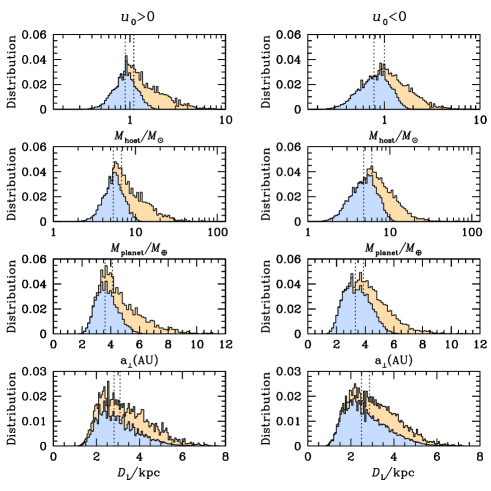
Figure 8: Bayesian posteriors for four physical parameters $(M_{\rm host},M_{\rm planet},a_{\perp},D_{L})$ obtained by applying constraints from the ground-only microlensing fit (Table 1) to simulated events from a Galactic model (yellow histograms). The blue histograms show the results of applying the lens-flux constraint: $D_{L}>2.31\,{\rm kpc}\,(M/M_{\odot})^{1.5}$ based on limits on the lens light from the blend. The $u_{0,\oplus}>0$ (left) and $u_{0,\oplus}<0$ (right) solutions are qualitatively similar, although the latter are generally broader, both before (yellow) and after (blue) the flux constraint is applied (blue).

Because we have measured both the microlens parallax ${\mbox{\boldmath$\pi$}}_{\rm E}$ and the Einstein radius $\theta_{\rm E}$ reasonably precisely, our main orientation has been to estimate the physical parameters using the microlensing (and CMD) parameters alone, supplemented by the flux constraint but without Galactic priors. However, it is of some interest to ask how the event would have been analyzed in the absence of Spitzer data.

We therefore next conduct a Bayesian analysis using only the ground-based data, i.e., ignoring the Spitzer data. We generally follow the procedures of Jung et al. (2018). We represent the outcome of the microlensing light-curve analysis by Gaussian errors for $t_{\rm E}$ (using Table 1) and $\theta_{\rm E}=1.56\pm 0.24\,{\rm mas}$ according to Equation (6). We represent the constraint on ${\mbox{\boldmath$\pi$}}_{\rm E}$ as a 2-D Gaussian derived from the left panels of Figure 6. Then we weight model Galactic events (as per Jung et al. 2018) according to these Gaussians. The results are shown as yellow contours in Figure 8. The resulting profiles are relatively broad, and they peak near the results shown in Table 6 derived from the ground+Spitzer analysis. For example, the median host mass for $(u_{0}>0)$ is $1.1\,M_{\odot}$ compared to $M_{\rm host}=1.36^{+0.25}_{-0.22}M_{\odot}$ in Table 6.

We then add a flux constraint (as in Section 6.2). The result is shown as blue contours in Figure 8. As expected, the effect is to sharply reduce the number of high-mass lenses. For example, the median host mass for $(u_{0}>0)$ becomes $0.88^{+0.27}_{-0.22}\,M_{\odot}$ compared to $M_{\rm host}=1.14^{+0.10}_{-0.12}M_{\odot}$ in Table 7. One may compare the $1\,\sigma$ ranges of the two sets of distributions directly in Tables 7 and 8. Overall the latter are two-to-four times broader, with peaks that are offset by less $<1\,\sigma$. That is, the result of the Spitzer parallax measurement is to much more precisely locate the solution (despite the absence of Galactic priors) within the region expected in the absence of Spitzer data (but with Galactic priors). The main effect of the Spitzer data is to exclude low mass lenses. But these low-mass (high $\pi_{\rm E}$) lenses are already significantly disfavored in the ground+Bayes analysis.

Table 8: Physical parameters from Bayesian analysis with flux constraint

Parameter	$u_{0}>0$	$u_{0}<0$
$M_{\rm host}$ $[M_{\odot}]$	$0.88_{-0.23}^{+0.27}$	$0.79_{-0.27}^{+0.32}$
$M_{\rm planet}$ $[M_{\oplus}]$	$5.35_{-1.38}^{+1.61}$	$4.75_{-1.61}^{+1.93}$
$a_{\perp}$ [au]	$3.60_{-0.69}^{+0.81}$	$3.31_{-0.89}^{+1.00}$
${\it D_{L}}$ [kpc]	$2.82_{-0.73}^{+1.12}$	$2.50_{-0.78}^{+1.22}$

8 Discussion

KMT-2018-BLG-0029Lb has the lowest planet-host mass ratio $q=0.18\times 10^{-4}$ of any microlensing planet to date. Although eight planets had previously been discovered in the range of 0.5–1.0$\times 10^{-4}$, including seven analyzed by Udalski et al. (2018) and one discovered subsequently (Ryu et al., 2019), none came even within a factor of two of the planet that we report here. This discovery therefore proves that the previously discovered pile-up of planets with Neptune-like planet-host mass ratios does not result from a hard cut-off in the underlying distribution of planets. However, it will require more than a single detection to accurately probe the frequency of planets in this sub-Neptune mass-ratio regime. It is somewhat sobering that after 16 years of microlensing planet detections there are only nine with well measured mass ratios $q\leq 1\times 10^{-4}$. Hence, it is worthwhile to ask about the prospects for detecting more.

8.1 Prospects for Very Low $q$ Microlensing Planets

Of the nine such events, five were found 2005–2013 and four were found 2016–2018. These two groups have strikingly different characteristics. Four (OGLE-2005-BLG-390, OGLE-2007-BLG-368, MOA-2009-BLG-266, and OGLE-2013-BLG-0341) from the first group revealed their planets via planetary caustics, and only one (OGLE-2005-BLG-169) via central or resonant caustics. By contrast, all four from the second group revealed their planets via central or resonant caustics and all with impact parameters $u_{0}{\lesssim}0.05$. Another telling difference is that follow-up observations played a crucial or very important role in characterizing the planet for four of the five in the first group, while follow-up observations did not play a significant role in characterizing any of the four planets in the second group. Finally, the overall rate of discovery approximately doubled from the first to the second period.

The second period, 2016–2018, coincides with the full operation of KMTNet in its wide-field, 24/7 mode (Kim et al., 2018b, c). The original motivation for KMTNet was to find and characterize low-mass planets without requiring follow-up observations (Kim et al., 2018a). All four planets from the second group were intensively observed by KMTNet, with the previous three all in high-cadence ($\Gamma=4\,{\rm hr}^{-1}$) fields and KMT-2018-BLG-0029Lb in a $\Gamma=1\,{\rm hr}^{-1}$ field. It should be noted that OGLE-2016-BLG-1195Lb was discovered and independently characterized (i.e., without any KMTNet data) by OGLE and MOA (Bond et al., 2017). In this sense, it is similar to OGLE-2013-BLG-0341LBb, which would have been discovered and characterized by OGLE and MOA data, even without follow-up data.

The above summary generally confirms the suggestion of Udalski et al. (2018) that the rate of low-mass planet discovery has in fact doubled in the era of continuous wide-field surveys. However, it also suggests that this discovery mode (i.e., without substantial follow-up observations) is “missing” many low-mass planets that were being discovered in the previous period. Apart from OGLE-2013-BLG-0341, which would have been characterized without follow-up, three of the other four low-mass planets from that period were all discovered in what would today be considered “outlying fields”, with Galactic coordinates $(l,b)$ of OGLE-2005-BLG-169 $(0.67,-4.74)$, OGLE-2007-BLG-368 $(-1.65,-3.69)$, MOA-2009-BLG-266 $(-4.93,-3.58)$. These regions are currently observed by KMTNet at $\Gamma=(1,1,0.4)\,{\rm hr}^{-1}$. Only OGLE-2005-BLG-390 $(2.34,-2.92)$ lies in what is now a high-cadence KMT field.

Moreover, the rate of discovery of microlensing events in these outlying fields is much higher today than it was when these four planets were discovered. Hence, while there is no question that the pure-survey mode has proved more efficient at finding low-mass planets, the rate of discovery could be enhanced by aggressive follow-up observations. See also Figure 8 from Ryu et al. (2020).

8.2 Additional Spitzer Planet

KMT-2018-BLG-0029Lb is the sixth published planet in the Spitzer statistical sample that is being accumulated to study the Galactic distribution of the planets (Yee et al., 2015; Calchi Novati et al., 2015). The previous five were OGLE-2014-BLG-0124Lb (Udalski et al., 2015a), OGLE-2015-BLG-0966Lb (Street et al., 2016), OGLE-2016-BLG-1190Lb (Ryu et al., 2017b), OGLE-2016-BLG-1195Lb (Bond et al., 2017; Shvartzvald et al., 2017), and OGLE-2017-BLG-1140Lb (Calchi Novati et al., 2018).

While it is premature to derive statistical implications from this sample, it is important to note that the planetary signature in the KMT-2018-BLG-0029 light curve remained hidden in the real-time photometry, although the pipeline re-reductions did yield strong hints of a planet. Nevertheless, TLC re-reductions were required for a confident signal. Hence, the history of this event provides strong caution that careful review of all Spitzer microlensing events, with TLC re-reductions in all cases that display possible hints of planets, will be crucial for fully extracting information about the Galactic distribution of planets from this sample.

8.3 High-Resolution Followup

As discussed in Section 6, the blended light is consistent with being generated by the lens. This identification would be greatly strengthened if the blend (which is about 2 mag brighter than the source in the $I$-band) were found to be astrometically aligned with the position of fhe microlensed source to the precision of high-resolution measurements. These could be carried out immediately using either ground-based adaptive optics (AO) or with the Hubble Space Telescope (HST). Even if such precise alignment were demonstrated, one would still have to consider the possibility that the blend was not the lens, but rather either a star that was associated with the event (companion to lens or source), or even a random field star that was not associated with the event. These alternate possibilities could be constrained by the observations themselves. For example, the blend’s color and magnitude might be inconsistent with it lying in the bulge. And the possibility that the blend was a companion to the lens could be constrained by the microlensing signatures to which such an object would give rise. The possibility that the blend is an ambient star could be estimated from the surface density of stars of similar brightness together the astrometric precision of the measurement. It is premature to speculate on the analysis of such future observations. The main point is that these observations should be taken relatively soon, before the lens and source substantially separate, so that their measured separation reflects their separation at the time of the event.

Even in the case that the relatively bright blend proves to be displaced from the lens, these observations would still serve as a first epoch to be compared to future high-resolution observations when the lens and source have significantly separated. If the lens is sufficiently bright, its identification could be confirmed after a relatively few years from, e.g., image distortion. In the worst case, the lens will not measurably add to the source flux, and so could only be unambiguously identified when it had separated about 1.5 FWHM from the source. This would occur $\delta t=3.2\,{\rm yr}(\lambda/1.1\,\mu{\rm m})(D/39{\rm m})^{-1}(\mu/3.3\,{\rm mas}\,{\rm yr}^{-1})^{-1}$ after the event, where $\lambda$ is the wavelength of observation and $D$ is the diameter of the mirror. Such observations would be feasible at first AO light on any of the extremely large telescopes (ELTs) but would have to wait until 2036 for, e.g., $1.6\,\mu{\rm m}$ observations on the Keck 10m telescope.

To assist in the interpretaion of such observations, we include auxiliary files with the $(x,y,I)$ data for field stars on the same system as the precision measurements for these quantities for the microlensed source, namely $(x,y,I)=(151.96,149.30,22.02)$.

9 Appendix: Spitzer Light-Curve Investigation

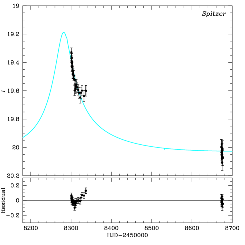
Figure 9: Full Spitzer light curve, including all 2018 and 2019 data. Compare to Figure 2, which shows the subset of these data used in the analysis. The truncated data set excludes the second-half-2018 data, i.e., HJD${}^{\prime}>8307$. The full data set shown here exhibits strong correlated residuals (high points at HJD${}^{\prime}>8307$), which then also induce high residuals in the first few points. Note that no such systematically high points are seen in Figure 2 because the model is freed from the necessity to try to fit the later correlated high points.

The full Spitzer light curve (i.e., all-2018 plus 2019) exhibits clear systematics, or more formally, residuals that are correlated in time and with rms amplitude well above their photon noise. This can be seen directly by comparing the full light curve (Figure 9) to the one analyzed in the main body of the paper (Figure 2). In addition to the clear correlated residuals in the latter, it also has an error renormalization factor (relative to the photon-noise-based pipeline errors) of 2.30 compared to 1.17 when the second-half-2018 data are removed.

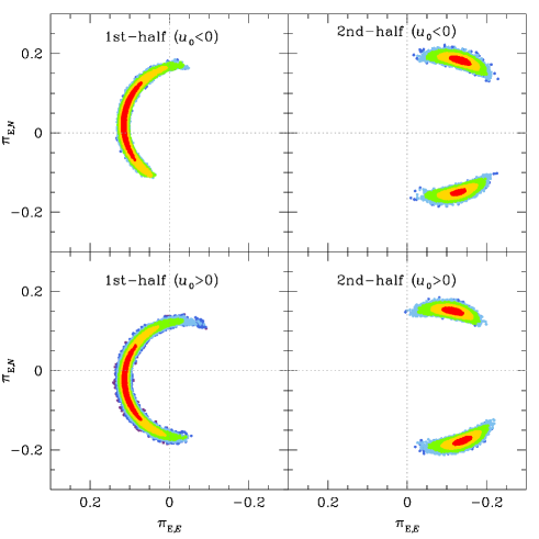
Figure 10: Spitzer-“only” parallax contours for two subsets of the data, either “1st-half” or “2nd-half” of 2018 Spitzer data together with all (i.e., one week) of 2019 (“baseline”) Spitzer data. The contours for $u_{0,\oplus}<0$ (upper) and $u_{0,\oplus}>0$ (lower) are similar, but the contours based on “1st-half” (left) and “2nd-half” (right) are very different. The tension between these two halves is a reflection of the correlated photometry errors as seen in Figure 9

A second way to view the impact of these correlated errors is to compare the Spitzer-“only” solution derived from combining first-half-2018 with 2019 data to the one derived from combining second-half-2018 with 2019 data. See Figure 10. While the upper $(u_{0}>0)$ and lower $(u_{0}<0)$ pairs of panels are similar, the left (first-half) and right (second-half) pairs of panels are radically different. They have completely different morphologies, and the contours themselves only overlap at the $3\,\sigma$ level.

Yet a third way to view the impact of these correlated errors is to “predict” the “baseline” Spitzer flux, $f_{\rm base}\equiv f_{s}+f_{b}$ from the full 2018 data set and then compare this with the measured $f_{\rm base}$ from 2019 data. this yields $3.0\pm 0.1$ versus $2.46\pm 0.03$.

While these are just different “viewing angles” of the same effects in the data, we present all three because they open different paths to trying to establish their origin. Any attempt to identify a physical cause for these effects must begin with a physical understanding of the measurement process together with the specific physical conditions of the measurment.

The data stream consists of six dithered exposures at each epoch, each of which yields a matrix of photo-electron counts from the detector. In contrast to optical CCDs, the PRF of the detector is highly non-uniform over the pixel surface, which means that the quantitative interpretation of the pixel counts in terms of incident photons requires relatively precise knowledge of the stellar positions in the frame of the detector matrix. This applies both to the target star as well as any other stars whose light profile (PSF) signficantly overlaps that of the target. We note that this would not be true if 1) one were interested in only relative photometry and 2) the detector position and orientation returned to the same sky position and orientation (or set of six sky positions and orientations) at each epoch. In that case, one could use a variant of DIA. However, neither condition applies to Spitzer microlensing observations. Most importantly, the observations typicaly span four to six weeks, during which the detector rotates by several degrees. In addition, one must actually know the target position in order to translate total photon counts into a reliable estimate of incident photons, which in turn is required to apply the $VIL$ (or $IHL$) color-color relation. This latter problem is usually solved with adequate precision. However, the impossibility of DIA, together with the constraints imposed by crowded fields, is what led to the development of a new PRF photometry algorithm (Calchi Novati et al., 2015).

This algorithm operates with several variants. For example, if the source is relatively bright at all epochs, then its position can be determined on an image-by-image basis. If it is bright at some epochs and not others, then the first group can be used to determine the source position relative to a grid of field stars, with this position then applied to the second group. If the source position cannot be determined at all from the Spitzer data (e.g., because the event is well past peak by the time the observations begin), then it can be found near peak from DIA of optical data relative to a grid of optical field stars. Then this optical grid can be cross-matched to Spitzer field stars, which leads to a prediction of the source position relative to the detector matrix. In general, one of more of these procedures works quite well for the great majority of Spitzer microlensing events that are subjected to TLC analysis.

However, for KMT-2018-BLG-0029, the conditions were especially challenging. First, the source flux (determined from the color-color relation) $f_{s,Spitzer}=0.58$ is quite small relative to that of three blends that lie within about 2 pixels, i.e., 40, 35, and 29. Second these bright blends overlap each other (and possibly other unresolved stars), and hence it is impossible to reliably determine their positions even from the higher-resolution ground-based data. (By contrast, although the source is much fainter than the neighboring blends, its position can be derived from ground-based DIA because it varies strongly.)

One initially plausible conjecture for the origin of the correlated errors would be that the photometry is more reliable when the source is brighter simply because its position is better determined on an epoch-by-epoch basis, and that the poorly known positions of the blends increasingly corrupt the measurements when the source is fainter. This conjecture would lead to the following “triage sequence” of confidence in the data: first-half-2018, second-half-2018, 2019, i.e., by decreasing brightness. Moreover, tests show that the target centroid can be constrained for almost all of the 2018 epochs based on Spitzer data alone, typically to within $\sim 0.1$ and $\sim 0.2$ pixels per epoch, for the first and second halves, respectively, but cannot be constrained at all for 2019. This line of reasoning would possibly lead to accepting all the 2018 data and rejecting the 2019 data on the grounds that the 2019 data were “most affected by systematics”.

We considered this approach but rejected it for reasons that are given in the next paragraph. Our main reason for recounting it in some detail is to convince the reader of its superficial plausibility and also of the danger of “explaining” evident correlated residuals by “phyiscal” arguments that are not rooted in the real physical conditions. We note that the interested reader can see the result of applying this approach by accessing the version of this paper that was prepared prior to the 2019 Spitzer microlensing season, i.e., when only 2018 data were available (arXiv:1906.11183). In fact, the final results derived from this 2018-only analysis do not differ dramatically from those presented in the body of this paper, although some of the intermediate steps look quite different.

The first point to note is that there is an immediate warning flag regarding this approach: the 2018-only light curve looks much worse (arXiv:1906.11183) than the first-half-2018-plus-2019 light curve and, correponding to this, has a much higher error-renormalization factor. This already suggests (although it hardly proves) that the real problems are concentrated in the second-half-2018 data. However, more fundamentally, the logic on which the conjecture is based does not hold up. The centroid position can be determined to better than 0.1 pixels by transforming from the optical frame, so the fact that this centroid can be determined to 0.2 pixels from the second-half-2018 data has no practical implication for the photometry. And in particular, the same correlations between the residuals remain for the second-half-2018 data whether the position is derived from Spitzer images alone or by transformation from the optical frame.

Another path toward understanding this issue, which proves to be more self-consistent, is to examine the photometry of the three bright blends as a function of time. In all three cases, the mean value and scatter are very similar when the first-half-2018 and 2019 data are compared. These are [($39.62\pm 0.13,0.51$) versus ($39.76\pm 0.16,0.61$)], [($34.74\pm 0.49,1.91$) versus ($35.22\pm 0.44,1.64$)], and [($28.90\pm 0.69,2.68$) versus ($28.76\pm 0.55,2.05$)] for the first, second, and third blend, respectively. That is, the means differ by $0.68\,\sigma$, $0.73\,\sigma$, and $0.16\,\sigma$, respectively. By contrast, both the first and third blend display strong “features” during $8310<{\rm HJD}^{\prime}<8338$. For the first blend, these data have a mean of $40.69\pm 0.20$, i.e., $5\,\sigma$ higher than predicted by the combined first-half-2018 and 2019 data: $39.68\pm 0.10$ For the third blend, these data have similar mean but a scatter (5.38) that is well over twice the values of the other two periods. This is strong empirical evidence that the first-half-2018 and 2019 data are rooted in a comparable physical basis, but the second-half-2018 data are not. Given that the field rotation, in combination with the severe crowding from several bright blends, provide a plausible physical explanation for these differences, we conclude that first-half-2018 and 2019 data can be analyzed as a single data set, but the second-half-2018 data must be excluded from the analysis.

References

- (1)
- Alard & Lupton (1998) Alard, C. & Lupton, R.H.,1998, ApJ, 503, 325
- Albrow et al. (2009) Albrow, M. D., Horne, K., Bramich, D. M., et al. 2009, MNRAS, 397, 2099
- Batista et al. (2011) Batista, V., Gould, A., Dieters, S. et al. 2011, A&A, 529, 102
- Batista et al. (2014) Batista, V., Beaulieu, J.-P., Gould, A., et al. 2014, ApJ, 780, 54
- Batista et al. (2015) Batista, V., Beaulieu, J.-P., Bennett, D.P., et al. 2015, ApJ, 808, 170
- Bennett et al. (2006) Bennett, D.P., Anderson, J., Bond, I.A., et al. 2006, ApJ, 647, L171
- Bennett et al. (2010) Bennett, D.P., Rhie, S.H., Nikolaev, S. et al. 2010, ApJ, 713, 837
- Bennett et al. (2015) Bennett, D.P., Bhattacharya, A., Anderson, J., et al. 2015, ApJ, 808, 169
- Bensby et al. (2013) Bensby, T. Yee, J.C., Feltzing, S. et al. 2013, A&A, 549A, 147
- Bessell & Brett (1988) Bessell, M.S., & Brett, J.M. 1988, PASP, 100, 1134
- Bhattacharya et al. (2017) Bhattacharya, A., Bennett, D.P., Anderson, J., et al. 2017, AJ, 154, 59
- Bond et al. (2004) Bond, I.A., Udalski, A., Jaroszyński, M. et al. 2004, ApJ, 606, L155
- Bond et al. (2017) Bond, I.A., Bennett, D.P., Sumi, T. et al. 2017, MNRAS, 469, 2434
- Calchi Novati et al. (2015) Calchi Novati, S., Gould, A., Yee, J.C., et al. 2015, ApJ, 814, 92
- Calchi Novati et al. (2019) Calchi Novati, S., Suzuki, D., Udalski, A., et al. 2019, AJ, 157, 121
- Calchi Novati et al. (2018) Calchi Novati, S., Skowron, J., Jung, Y.K. , et al. 2018,
- DePoy et al. (2003) DePoy, D.L., Atwood, B., Belville, S.R., et al. 2003, SPIE 4841, 827
- Dong et al. (2007) Dong, S., Udalski, A., Gould, A., et al. 2007, ApJ, 664, 862
- Dong et al. (2009) Dong, S., Gould, A., Udalski, A., et al. 2009, OGLE-2005-BLG-071Lb, ApJ, 695, 970
- Gaudi (1998) Gaudi, B.S. 1998, ApJ, 506, 533
- Gaudi et al. (2008) Gaudi, B.S., Bennett, D.P., Udalski, A. et al. 2008, Science, 319, 927
- Gonzalez et al. (2012) Gonzalez, O. A., Rejkuba, M., Zoccali, M., et al. 2012, A&A, 543, A13
- Gould (1992) Gould, A. 1992, ApJ, 392, 442
- Gould (1994) Gould, A. 1994, ApJL, 421, L75
- Gould (2000) Gould, A. 2000, ApJ, 542, 785
- Gould (2003) Gould, A. 2003, 2003astro.ph.10577
- Gould (2004) Gould, A. 2004, ApJL, 606, 319
- Gould (2019) Gould, A. 2019, JKAS, 52, 121
- Gould & Yee (2012) Gould, A. & Yee, J.C. 2012, ApJ, 755, L17
- Gould et al. (2014) Gould, A., Udalski, A., Shin, I.-G. et al. 2014, Science, 345, 46
- Gould et al. (2013) Gould, A., Carey, S., & Yee, J. 2013, 2013spitz.prop.10036
- Gould et al. (2014) Gould, A., Carey, S., & Yee, J. 2014, 2014spitz.prop.11006
- Gould et al. (2015a) Gould, A., Yee, J., & Carey, S., 2015a, 2015spitz.prop.12013
- Gould et al. (2015b) Gould, A., Yee, J., & Carey, S., 2015b, 2015spitz.prop.12015
- Gould et al. (2016) Gould, A., Yee, J., & Carey, S., 2016, 2015spitz.prop.13005
- Gould et al. (1994) Gould, A., Miralda-Escudé, J. & Bahcall, J.N. 1994, ApJ, 423, L105
- Han et al. (2016) Han, C., Udalski, A., Lee, C.-U., et al. 2016, ApJ, 827, 11
- Holtzman et al. (1998) Holtzman, J.A., Watson, A.M., Baum, W.A., et al. 1998, AJ, 115, 1946
- Hwang et al. (2018) Hwang, K.-H., Udalski, A., Shvartzvald, Y. et al. 2018, AJ, 155, 20
- Jiang et al. (2005) Jiang, G., DePoy, D.L., Gal-Yam, A., et al. 2005, ApJ, 617, 1307
- Jung et al. (2018) Jung, Y. K., Udalski, A., Gould, A., et al. 2018, AJ, 155, 219
- Jung et al. (2019a) Jung, Y. K., Gould, A., Zang, W., et al. 2019a, AJ, 157, 72
- Jung et al. (2019b) Jung, Y. K., Gould, A., Udalski, A, et al. 2019b, AJ, 158, 28
- Kervella et al. (2004) Kervella, P., Thévenin, F., Di Folco, E., & Ségransan, D. 2004, A&A, 426, 297
- Kim et al. (2016) Kim, S.-L., Lee, C.-U., Park, B.-G., et al. 2016, JKAS, 49, 37
- Kim et al. (2018a) Kim, D.-J., Kim, H.-W., Hwang, K.-H., et al., 2018a, AJ, 155, 76
- Kim et al. (2018b) Kim, H.-W., Hwang, K.-H., Kim, D.-J., et al., 2018b, AJ, 155, 186
- Kim et al. (2018c) Kim, H.-W., Hwang, K.-H., Kim, D.-J., et al., 2018c, arXiv:1804.03352
- Kim et al. (2018d) Kim, H.-W., Hwang, K.-H., Shvartzvald, et al. 2018d, arXiv:1806.07545
- Koshimoto & Bennett (2019) Koshimoto, N. & Bennett, D.P., 2019, AJ, submitted, arXiv:1905.05794
- Muraki et al. (2011) Muraki, Y., Han, C., Bennett, D.P., et al. 2011, ApJ, 741, 22
- Minniti et al. (2017) Minniti, D., Lucas, P., VVV Team, 2017, yCAT 2348, 0
- Nataf et al. (2013) Nataf, D.M., Gould, A., Fouqué, P. et al. 2013, ApJ, 769, 88
- Paczyński (1986) Paczyński, B. 1986, ApJ, 304, 1
- Park et al. (2004) Park B.-G., DePoy, D.L., Gaudi, B.S. et al. 2004, ApJ, 609, 166
- Refsdal (1966) Refsdal, S. 1966, MNRAS, 134, 315
- Ryu et al. (2017b) Ryu, Y.-H., Yee, J.C., Udalski, A.,, et al. 2017b, AJ, 155, 40
- Ryu et al. (2019) Ryu, Y.-H., Udalski, A., Yee, J.C. et al. 2019, OGLE-2018-BLG-0532Lb: Cold Neptune With Possible Jovian Sibling, AAS submitted, arXiv:1905.08148
- Ryu et al. (2020) Ryu, Y.-H., Navarro, M.G., Gould, A. et al. 20202, AJ, in press
- Schechter et al. (1993) Schechter, P.L., Mateo, M., & Saha, A. 1993, PASP, 105, 1342
- Shin et al. (2018) Shin, I.-G., Udalski, A., Yee, J.C., et al. 2018, ApJ, 863, 23
- Shvartzvald et al. (2017) Shvartzvald, Y., Yee, J.C., Calchi Novati, S. et al. 2017b, ApJL, 840, L3
- Skowron et al. (2011) Skowron, J., Udalski, A., Gould, A et al. 2011, ApJ, 738, 87
- Smith et al. (2003) Smith, M., Mao, S., & Paczyński, B., 2003, MNRAS, 339, 925
- Street et al. (2016) Street, R., Udalski, A., Calchi Novati, S. et al. 2016, ApJ, 829, 93.
- Suzuki et al. (2016) Suzuki, D., Bennett, D.P., Sumi, T., et al. 2016, ApJ, 833, 145
- Tomaney, & Crotts (1996) Tomaney, A.B., & Crotts, A.P.S. 1996, AJ, 112, 2872
- Udalski (2003) Udalski, A. 2003, Acta Astron., 53, 291
- Udalski et al. (1994) Udalski, A.,Szymanski, M., Kaluzny, J., Kubiak, M., Mateo, M., Krzeminski, W., & Paczyński, B. 1994, Acta Astron., 44, 227
- Udalski et al. (2015a) Udalski, A., Yee, J.C., Gould, A., et al. 2015a, ApJ, 799, 237
- Udalski et al. (2015b) Udalski, A., Szymański, M.K. & Szymański, G. 2015b, Acta Astronom., 65, 1
- Udalski et al. (2018) Udalski, A., Ryu, Y.-H., Sajadian, S., et al. 2018, Acta Astron., 68, 1
- Woźniak (2000) Woźniak, P. R. 2000, Acta Astron., 50, 421
- Yee et al. (2015) Yee, J.C., Gould, A., Beichman, C., 2015, ApJ, 810, 155
- Yoo et al. (2004) Yoo, J., DePoy, D.L., Gal-Yam, A. et al. 2004, ApJ, 603, 139
- Zhu et al. (2017) Zhu, W., Udalski, A., Calchi Novati, S. et al. 2017, AJ, 154, 210