Detecting Gravitational Self Lensing from Stellar-Mass Binaries Composed of Black Holes or Neutron Stars

Abstract

We explore a unique electromagnetic signature of stellar-mass compact-object binaries long before they are detectable in gravitational waves. We show that gravitational lensing of light emitting components of a compact-object binary, by the other binary component, could be detectable in the nearby universe. This periodic lensing signature could be detected from present and future X-ray observations, identifying the progenitors of binaries that merge in the LIGO band, and also unveiling populations that do not merge, thus providing a tracer of the compact-object binary population in an enigmatic portion of its life. We argue that periodically repeating lensing flares could be observed for $\mathrel{\hbox to0.0pt{\lower 4.0pt\hbox{\hskip 1.0pt$\sim$}\hss}\raise 1.0pt\hbox{$<$}}100$ ks orbital-period binaries with the future Lynx X-ray mission, possibly concurrent with gravitational wave emission in the LISA band. Binaries with longer orbital periods could be more common and be detectable as single lensing flares, though with reliance on a model for the flare that can be tested by observations of succeeding flares. Non-detection of such events, even with existing X-ray observations, will help to constrain the population of EM bright compact-object binaries.

1 Introduction: Lensing Happens

The detection of the merger of eleven compact-object (CO) binaries by the Laser Interferometer Gravitational-Wave Observatory (LIGO) (Abbott et al., 2016b, c, 2017a, 2017e, 2017b, 2017c; The LIGO Scientific Collaboration et al., 2018) has begun to shape our understanding of binary black hole (BBH) and binary neutron star (BNS) demographics (e.g., Abbott et al., 2016a, 2017d; The LIGO Scientific Collaboration et al., 2018). While ongoing monitoring of the high-frequency gravitational-wave (GW) sky with LIGO will continue to enhance our understanding of these fascinating systems, detection at merger offers only a snapshot in a binary’s lifetime. A snapshot from which we aim to infer the entire life story of a population of CO-binary systems: the mechanisms that form the binaries and eventually drive them towards merger. Here we offer a possible electromagnetic (EM) mechanism with the potential to diversify the demographic sample of CO binaries to include those at an earlier stage of evolution: outside of the LIGO and the lower GW-frequency LISA (Amaro-Seoane et al., 2017) snapshots, prior to strong GW emission.

On the theoretical side, proposed mechanisms for the formation of binaries that will merge in the LIGO band involve a variety of astrophysical processes that are still uncertain. The two most highly studied channels for forming LIGO binaries are isolated evolution of massive binary-star systems in the ‘field’ via the common-envelope (e.g., Voss & Tauris, 2003; Dominik et al., 2012, 2013; Ivanova et al., 2013; Dominik et al., 2015; Belczynski et al., 2016b; Belczynski et al., 2016a) and chemically homogeneous evolution (de Mink & Mandel, 2016; Mandel & de Mink, 2016; Marchant et al., 2016) scenarios, and dynamical formation in dense cluster environments (e.g., Portegies Zwart & McMillan, 2000; Banerjee et al., 2010; Tanikawa, 2013; Bae et al., 2014; Rodriguez et al., 2015; Rodriguez et al., 2016a; Askar et al., 2017; Park et al., 2017), or via secular dynamical interactions such as the Kozai-Lidov mechanism (Antonini & Perets, 2012; Naoz, 2016; Silsbee & Tremaine, 2017; Antonini et al., 2017; Randall & Xianyu, 2018; Zhang et al., 2019). With other possible scenarios involving very massive stars, AGN discs, or primordial black holes (BHs; Fryer et al., 2001; Loeb, 2016; Bird et al., 2016; Stone et al., 2017; Bartos et al., 2017; McKernan et al., 2018; D’Orazio & Loeb, 2018).

To determine which channels dominate, and to gain insight into the astrophysics regulating each channel, we must aim to determine in what proportion the proposed formation and merger mechanisms contribute to the observed CO merger rate. Achieving this relies on predicting unique imprints of formation channels on binary properties during an observable portion of their lifetimes. Such properties include mass and spins at inspiral and merger (Gerosa et al., 2013; Kesden et al., 2015; Gerosa et al., 2015; Rodriguez et al., 2016b; Gerosa & Berti, 2017; Fishbach et al., 2017; Liu & Lai, 2017; Rodriguez et al., 2018b; Rodriguez & Antonini, 2018), redshift distributions (Rodriguez & Loeb, 2018; Rodriguez et al., 2018a), eccentricities measured near merger in the LIGO band and also earlier in the binary evolution, with lower frequency GWs from LISA, as well as comparison of populations across the LIGO and LISA bands (D’Orazio & Loeb, 2018; Samsing et al., 2018; Samsing & D’Orazio, 2018; D’Orazio & Samsing, 2018; Gerosa et al., 2019). With the exception of recent work (Samsing et al., 2019; Kremer et al., 2019a), the majority of methods for measuring such binary properties can only be employed near merger, when GW emission is detectable, or when strong EM transients associated with merger may operate (e.g., explosions related to NS mergers Abbott et al., 2017c).

In this work we propose an EM signature of CO binaries that would act as a tracer of CO binary formation and evolution long before detection is possible in GWs. We propose an EM tracer caused by binary self-lensing whereby at least one component of the CO binary is bright and is periodically magnified by its companion via gravitational lensing. Such an EM signature would be uniquely periodic while having the benefit of being a magnified source of intrinsic emission. This unique EM signature would provide another handle on CO-binary populations in a regime complimentary to GW observations, helping to vet formation and merger scenarios. It is possible (though less-likely) that binary self-lensing could also serve as an EM counterpart to future GW observations with the space-based LISA.

In Section 2 we consider the spatial and time scales associated with lensing, in calculations that apply to any pair of merging COs, whether they consist of NSs, stellar mass BHs, or supermassive BHs. In this work we focus on CO binaries that, if they merge, would generate gravitational waves in the LIGO band. We have considered the case of supermassive BHs in a previous work (D’Orazio & Di Stefano, 2018).

In Section 3, we consider the optimal binary parameters for generating high magnification lensing flares that could be found to repeat over the course of a single or a few X-ray observations ($\mathrel{\hbox to0.0pt{\lower 4.0pt\hbox{\hskip 1.0pt$\sim$}\hss}\raise 1.0pt\hbox{$<$}}10^{2}$ ks). We further generate mock X-ray light curves for hypothetical nearby sources accreting at the Eddington limit and observed with Chandra-like, or future Lynx-like X-ray telescopes.

In Section 4 we estimates the number of CO binary systems that we expect to be EM bright at orbital periods and inclinations that can be probed by existing and future X-ray observations (as motivated in §3). We further consider mechanisms for lighting up the binary components, namely accretion from supernova fall-back or a common-envelope stage, or gas overflow from a tertiary stellar companion. In §5 we conclude with a discussion of what we may learn from lensing observations of CO binaries and in §6 we conclude.

2 Binary Self-Lensing: Spatial and Time Scales

We consider a binary consisting of two masses, $M_{1}$ and $M_{2}$, on a circular orbit with semimajor axis $a$, mass ratio $q=M_{2}/M_{1}\leq 1$, and total mass $M=M_{1}+M_{2}$. The Schwarzschild radius associated with the total mass is

$$R_{\rm S,T}=\frac{2GM}{c^{2}}.$$ (1)

A natural unit of time is

$${\cal T}_{\rm T,cross}=\frac{R_{\rm S,T}}{c},$$ (2)

the time required for light to traverse a distance equal to the Schwarzschild radius associated with $M$.

The semimajor axis may be expressed in units of $R_{\rm S,T}$: $a=N_{a}\,R_{\rm S,T}$. The orbital period is

$$P_{\rm orb}={\cal T}_{\rm T,cross}\,\Bigg{[}2\,\sqrt{2}\,\pi\,\,N^{3/2}_{a}\Bigg{]}.$$ (3)

The time to merger is

$$\tau_{\rm merge}={\cal T}_{\rm T,cross}\,\Bigg{[}\frac{5}{32}\,\frac{(1+q)^{2}}{q}\,\Big{(}N^{4}_{a}-N_{a,\rm merge}^{4}\Big{)}\Bigg{]}.$$ (4)

The ratio between the time to merge and the orbital period is

$$\frac{\tau_{\rm merge}}{P_{\rm{orb}}}=\Big{(}\frac{5}{64\,\sqrt{2}\,\pi}\Big{)}\,\Big{(}\frac{(1+q)^{2}}{q}\Big{)}\,N^{5/2}_{a}.$$ (5)

To incorporate lensing, we consider the Einstein radius, which depends on the line-of-sight distance, $a_{p}(t)$, between the lens and source. The distance from the observer to the binary may range from several parsecs to hundreds of Mpc, while the source and lens are in a compact binary. Hence, because the source-lens distance is much smaller than the distance to the binary, we can write the Einstein radius of each component of the binary, $R_{E,i}$ as follows,

$$R_{E,i}=\Bigg{(}2\,a_{p}(t)\,R_{S,i}\Bigg{)}^{1/2}=R_{S,T}\,\,\Big{(}2\,g(t)\,f_{i}(q)\Big{)}^{1/2}\,N^{1/2}_{a}.$$ (6)

Here, $g(t)$ is needed to include the orbital phase dependence of the line-of-sight separation between source and lens, and $f_{i}(q)$ includes the relationship between $R_{S,i}$ and $R_{S,T}$ (See for example Eq. (1) of D’Orazio & Di Stefano, 2018).

The effects of lensing depend on $u(t)$, the projected distance between the source of light and the foreground lens mass expressed in units of $R_{\rm E,i}.$ The magnification of a point source by a point lens is $1.34,$ when $u=1.$ For much smaller values of $u,$ the magnification is $1/u.$ If the lensed object is a NS, the light that is deflected is most likely to come from near the surface of the neutron star: $R_{\rm source}=R_{\rm NS}$. If the lensed object is a BH, light to be deflected may come from the region near the innermost stable circular orbit (ISCO) at $R_{\rm source}=3\,R_{\rm S,j}.$ To avoid finite-source-size effects that lead to lower magnification, we require $u>(1+\epsilon)\times R_{\rm source}/R_{\rm E,i}$, Thus, the maximum magnification possible, $\mathcal{M}_{\rm{max}}$, is

$$\mathcal{M}_{\rm{max}}=\frac{R_{\rm E,i}}{R_{\rm source}\,(1+\epsilon)}=N^{1/2}_{a}\,\frac{(2\,g(t)\,f(q))^{1/2}\,R_{S,T}}{(1+\epsilon)\,R_{\rm source}}.$$ (7)

This peak magnification occurs when the line-of-sight separation between the source and lens is at its maximum, and it repeats once per orbital period.

We can estimate the duration of the periodic lensing events to be $\tau_{\rm ev}=2R_{E,i}/v_{\rm orb}$,

$$\tau_{\rm ev}={\cal T}_{\rm T,cross}\,4\,\Big{(}g(t)\,f(q)\Big{)}^{1/2}\,N_{a}.$$ (8)

The duty cycle is the fraction of the orbital period during which an event is ongoing,

$${\cal D}=\Big{(}\frac{1}{\pi}\Big{)}\,\Big{(}2N_{a}\Big{)}^{-1/2}\,\Big{(}g(t)\,f(q)\Big{)}^{1/2}.$$ (9)

The time during which detectable effects occur may be either longer than or shorter than $\tau_{\rm ev}$, since depending on the situation, the value of $u$ needed to produce detectable magnification may be either larger than or smaller than $u=1.$

We can only detect the effects of lensing if the orbit is well-aligned with our line of sight. The probability that the alignment is suitable is approximately equal to

$${\cal P}=\frac{R_{E,L}}{a}=N^{-1/2}_{a}\,\Big{(}2\,g(t)\,f(q)\Big{)}^{1/2},$$ (10)

where suitable here means that $u\leq 1$.

The probability that the source is aligned within an inclination that gives $\mathcal{M}_{\rm{max}}$ is lower and given, for $R_{\rm source}\ll a$, by

$${\cal P}_{\mathcal{M}_{\rm{max}}}\sim\frac{2}{\pi}\frac{R_{\rm source}}{a}=\frac{2}{\pi}\frac{\cal P}{\mathcal{M}_{\rm{max}}}=\frac{2}{\pi}\frac{(1+\epsilon)R_{\rm source}}{R_{S,T}}N^{-1}_{a}\sim N^{-1}_{a}.$$ (11)

For choice of $R_{\rm source}=3R_{S,j}$, which is approximately the NS radius and the size of the BH ISCO, then ${\cal P}_{A\rm{max}}\sim N^{-1}_{a}$ is only approximate up to a factor of $(1+q)^{-1}$ for the primary lens and $(1+1/q)^{-1}$ for the secondary lens.

In Figure 1 we show the relationship between the orbital period and quantities relevant for detection. For each of four binary masses (left panel) and four binary mass ratios (right panel), Figure 1 shows, from top to bottom: the maximum magnification, the duration of the lensing event, the time to merger via gravitational wave emission, and the probability for alignment suitable for strong lensing Eq. (10).

We have selected a region, marked by two parallel vertical lines, corresponding to orbital periods between 100 ks and 200 ks. X-ray observations of external galaxies can cover comparable time intervals, often in separate exposures, possibly even by different X-ray telescopes. Some galaxies within $10-20$ Mpc have been observed for more than 5 times as long. If the total exposure time is larger than an orbital period there is a good chance of detecting a lensing spike multiple times. Thus, in the region in-between and to the left of the parallel lines, the lensing hypothesis would be most easily testable through a repeating signature.

To the right of the parallel lines, a single flare may still be detected and identified as a lensing candidate, to be followed up with future observations. These longer orbital-period binaries have longer lasting flares ($\mathrel{\hbox to0.0pt{\lower 4.0pt\hbox{\hskip 1.0pt$\sim$}\hss}\raise 1.0pt\hbox{$>$}}100$ sec) and higher maximum magnifications ($\mathrel{\hbox to0.0pt{\lower 4.0pt\hbox{\hskip 1.0pt$\sim$}\hss}\raise 1.0pt\hbox{$>$}}100$), making individual events more likely to be detected and potentially providing enough counts over a long enough time interval to allow reliable model fits. These longer orbital period systems also have a longer GW-driven time to merger (longer than the Hubble time). Note, however, that if, for example, mass transfer from a star in a hierarchical orbit is providing the mass that makes one or both compact objects detectable, mass transfer and mass loss from the system will likely decrease the time to merger so that some of these systems will merge in a Hubble time. Finally, the longer orbital period systems have a lower probability for optimal lensing alignment. In addition, for systems where less than an entire orbit is observed and the cadence of observation is longer than the event duration, the complete expression for the probability must include a factor equal to the observing duty cycle, which is smaller than unity in such systems. The reason we nevertheless expect that compact-object binaries with large orbital periods can contribute is that in each galaxy, the numbers of compact-object binaries with larger orbits and with lower intrinsic luminosities (that may be detectable with large magnification) is potentially large (See §4).

Looking at the variation with total binary mass in the left panel of Figure 1, we find that the lower mass systems produce shorter events with higher maximum magnification. Here the black, blue, green, and red lines represent equal mass binaries with total masses $4{M_{\odot}}$, $20{M_{\odot}}$, $100{M_{\odot}}$, $200{M_{\odot}}$ respectively. The lifetime of such systems under GW-driven decay is of order a Hubble time for the 100 ks orbital period, $4{M_{\odot}}$ binaries. The lifetime drops to $\sim 10^{8}$ yr for $100{M_{\odot}}$ binaries with 100 ks orbital periods. Hence, the less massive CO binaries exhibit shorter lensing durations but longer binary lifetimes and higher peak magnifications at the orbital periods of interest.

In the right panel of Figure 1, we plot the same quantities, but each curve corresponds to a different mass ratio. Each binary has a lens component with $M=100\,M_{\odot}$, and a second component that is of $1\,M_{\odot},10\,M_{\odot},50\,M_{\odot}$, and $100\,M_{\odot}$ in black, blue, green, and red, respectively (in the top panel, the uppermost curve is black, then blue, green, and red, respectively). We consider the situation in which the higher mass object lenses the inner disc of the accretion flow onto the smaller mass. This means that the Einstein radius is relatively large compared with the X-ray bright region of the disc around the smaller mass. This allows the maximum magnification to be larger for smaller mass ratio systems. Thus, the top panel shows the most interesting effect, while the three panels below illustrate that the rest of the parameters are weakly dependent on the binary mass ratio. We explore the ideal systems for detection in the next section.

$\begin{array}[]{cc}\includegraphics[scale={0.4}]{real_porb}&\includegraphics[scale={0.4},angle={0}]{real_porbq}\end{array}$

Figure 1: Binary self-lensing quantities vs. the binary orbital period in days. From top to bottom: the maximum possible magnification, the duration of a self-lensing event in seconds, the time until merger due to gravitational radiation in units of the Hubble time, and the strong-lensing probability, Eq (10). In the left panel we consider four equal-mass compact-object binaries with total masses $4{M_{\odot}}$, $20{M_{\odot}}$, $100{M_{\odot}}$ and $200{M_{\odot}}$ (black, blue, green, and red respectively, appearing from top to bottom in the top panel). In the right panel we vary the binary mass ratio for a fixed primary mass of $100{M_{\odot}}$ (assumed to be the lens). In order of appearance from top to bottom in each panel, are the mass ratios, $q=0.01,0.02,0.1,1.0$ (black, blue, green, and red respectively). Vertical black lines denote 100 ks and 200 ks orbital periods.

3 Which Systems can be Detected?

Figure 2 demonstrates the range of binary parameters for which observations are viable assuming an equal mass ratio binary and a source distance of 30 Mpc for a present-day, Chandra-like X-ray telescope (Evans et al., 2010), and at 300 Mpc for a future, Lynx-like telescope (Gaskin et al., 2018).

The teal shaded region labeled $\mathcal{C}\tau_{\rm{ev}}\geq 1$ estimates where the magnified number of counts for either telescope would be larger than one per lensing event duration. This timescale limitation is enforced to ensure that the lensing flare can be resolved, and observed to repeat. Longer integration times could of course allow deeper observations, but at the price of washing out the distinguishing flare. The duration of the lensing event $\tau_{\rm{ev}}$ is computed from Eq. (8). The lensed count rate is given by,

$$\mathcal{C}=\mathcal{C}_{0}\mathcal{M}_{\rm{max}},$$ (12)

where $\mathcal{M}_{\rm{max}}$ is given by Eq. (7) and the un-lensed count rate $\mathcal{C}_{0}$ is found by assuming that the source emits with a bolometric luminosity at a fraction $f_{\rm{Edd}}$ of the Eddington value at a distance $d$, and that all emission is in the $2-10$ kev range. Using the NASA HEASEARC WebPIMMS tool for the Chandra ACIS-S instrument, we find,

$$\mathcal{C}_{0}\approx 1.3\ \rm{cnt}\ \rm{s}^{-1}f_{\rm{Edd}}\left(\frac{d}{1\rm{Mpc}}\right)^{-2}\left(\frac{M}{10{M_{\odot}}}\right).$$ (13)

where we have adopted a galactic neutral Hydrogen column density of $n_{H}=1.22\times 10^{21}$ cm^-2 and a photon index of $2.0$ (Yang et al., 2015). We then simply scale the count rate with binary mass and distance.

The orange shaded region in Figure 2 demonstrates a range of feasible binary orbital periods for detection of repeating flares (corresponding to the region to the left of the vertical lines in Figure 1). To maximise the probability of seeing a lensing flare, we would like the orbital period to be short enough to observe over the course of a few observations. Hence, we draw a maximum orbital period at $10^{2}$ ks. For visualization purposes, we extend the orange region down to a minimum period of 1 ks, a standard single observation time for X-ray observatories. The lower limit of the orange shaded region is not a hard cutoff. Rather, there are a number of factors that affect the minimum observable orbital period for which observation of a lensing event is possible. We estimate this hard cutoff to be where the lensing duration is approximately the instrument readout time, $\approx 3.2$ seconds for Chandra. The gray lines in the left panel of Figure 2 are drawn at constant lensing flare duration, including this instrumental lower limit. The minimum orbital period is also set by the count-rate requirement delineated by the teal region, which extends below the 1 ks period limit for the most massive binaries. Hence, it is a combination of observed source brightness and instrumental cadence that determine the shortest orbital period systems for which lensing flares are detectable.

While the shorter orbital-period binaries are likely more rare, provide less magnification, and exhibit shorter event durations, they do offer a higher probability of lensing per binary. On the right $y$-axes of the left panel of Figure 2 we label the approximate probability of seeing a lensing event at the maximum magnification (Eq. 11). Note that the probability of seeing a lower magnification flare, given by Eq. (10), is higher than this and scales with $N^{-1/2}$ rather than $N^{-1}$. These probabilities of course do not take into account the binary population as a function of orbital separation and mass. Because closer separation and higher mass binaries merge more quickly (at least for GW-decay driven binaries), the probability of seeing a binary at a smaller separation also goes down, mitigating the higher lensing probabilities. Also, none of the considerations thus far take into account the time that the binary is EM bright. We address these issues in §4.

The hatched purple and gray regions in Figure 2 represent the approximate location of the LISA (GW frequencies $10^{-3}-10^{-1}$ Hz) and LIGO (GW frequencies $>10$ Hz) sensitivity ranges for circular-orbit binaries. For highly eccentric binaries, such as those that may form in dense stellar environments, these shaded regions would be shifted upwards because a binary with high eccentricity, but otherwise the same orbital period, emits the majority of its GW power at higher harmonics of the binary orbital frequency than in the circular case. We note that the lensing flare duration will also change by an amount less than $(1\pm e)$, while the magnification will change by an amount less than $\sqrt{1\pm e}$ for binary eccentricity $e$, depending on whether the lensing flare occurs closer to apocentre or pericentre. The periodic nature and symmetric nature of the lensing flare will not change for eccentric systems (Hu et al., 2019).

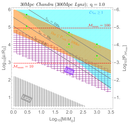
Figure 2: Regions in binary separation $a$ (in units of Schwarzschild radius of the total binary mass) and total-binary-mass space where lensing flares could be observable with a Chandra-like (Lynx-like) X-ray observatory at a distance of 30 Mpc (300 Mpc), assuming sources emit at the Eddington luminosity for their total binary mass. The teal region is where the instrument can detect at least one count per lensing flare duration. The orange region delineates binaries with orbital periods between $1-10^{2}$ ks. The gray lines are contours of constant lensing timescale, the shortest is set to the Chandra read-out time. The dashed red lines are lines of constant, maximum lensing magnification (Eq. 7). The right $y$-axis estimates the probability that a given binary will produce lensing at the maximum magnification, when observed for an entire orbital period. For reference, we draw the approximate regions of sensitivity for GW detection by LISA (GW frequencies of $10^{-3}-10^{-1}$ Hz, hatched purple) and LIGO (GW frequencies $>10$ Hz, hatched gray), assuming a binary on a circular orbit.

$\begin{array}[]{ccc}\includegraphics[scale={0.25}]{ex1_LC_3Mpc}&\includegraphics[scale={0.25}]{ex2_LC_30Mpc}&\includegraphics[scale={0.25}]{ex3_LC_30Mpc}\\ \includegraphics[scale={0.25}]{ex4_LC_3Mpc}&\includegraphics[scale={0.25}]{ex5_LC_30Mpc}&\includegraphics[scale={0.25}]{ex6_LC_30Mpc}\end{array}$

Figure 3: Simulated Chandra light curves of six different binary systems, zoomed in on the lensing flare. Each color represents one of the 100 realizations of the light curve, the spread of counts at each epoch gives an approximate uncertainty. Each panel corresponds to the binary parameters marked in the left panel of Figure 2 by green dots labeled ‘ex $\#$’.

Figure 3 shows example light curves from the specified locations in binary parameter space denoted in Figure 2 (labeled green dots). The axes are labeled in units of expected counts from a Chandra-like instrument for an Eddington luminosity source at the denoted distance, or a Lynx-like instrument with the same source at $10\times$ that distance. Each panel in Figure 3 zooms in on the flare caused by lensing of an emission region bound to one of the COs (we assume equal masses).

To compute the light curves we use the point source Doppler-boost plus lensing models found in §2.3 of (D’Orazio & Di Stefano, 2018). Denoting the Doppler+lensing magnification model $\mathcal{M}(t)$, the expected number of counts $K$ is found from randomly sampling the Poisson distribution,

$$\mathcal{P}(K)=\frac{(t_{\rm{bin}}\mathcal{C}_{0}\mathcal{M}(t))^{K}}{K!}\exp{\left[-t_{\rm{bin}}\mathcal{C}_{0}\mathcal{M}(t)\right]},$$ (14)

where $t_{\rm{bin}}$ is the bin size and $\mathcal{C}_{0}$ is in units of counts per second. Then $\mathcal{P}(K)$ provides the probability of detecting $K$ counts per $t_{\rm{bin}}$ given the average number of expected counts per bin $t_{\rm{bin}}\mathcal{C}_{0}\mathcal{M}(t)$.

In Figure 3, we plot a solid grey line to represent the magnification model, $t_{\rm{bin}}\mathcal{C}_{0}\mathcal{M}(t)$, and we plot scattered points to represent the expected counts drawn from the Poisson distribution. We realize the expected light curve 100 times (each realization denoted by a different color) to give an indication of the uncertainty at each observation time and, hence, the prospect of discerning the lensing flare. For each light curve we assume an equal mass ratio binary where each binary component has the same intrinsic luminosity. This implies that the lensing flare occurs twice per orbital period, but also that the lensing flare is less magnified than it would be in the case where only one of the binary components is bright. For the same reason, other sources of emission that are not lensed, such as that from a disk surrounding the binary, would further decrease the magnification of the flares shown in Figure 3 (see also D’Orazio et al., 2015, where the same issue is discussed in context of the orbital Doppler boost).

Figure 3 illustrates the distances to which lensing flares could be identified from different types of binaries. For BNS systems within $\sim 3$ Mpc ($30$ Mpc), a Chandra-like (Lynx-like) X-ray telescope could identify X-ray lensing flares, even when binning data over short, 10 second intervals needed to temporally resolve the lens flare. For more massive binaries, the longer flare duration and brighter intrinsic luminosity allows identification to farther distances. A Chandra-like (Lynx-like) instrument can identify lensing flares from $\approx 10^{2}-10^{3}{M_{\odot}}$ binaries out to $\sim 30$ $(300)$ Mpc. Using longer duration time bins could allow detection out to even farther distances than considered in Figure 3, but at the cost of washing out the lensing flare for short orbital period systems. We now turn towards estimating the number of binaries within these distances, and in the preferred range of orbital periods delineated in Figure 2.

4 Plausibility of detection

In this section we determine the plausibility of detecting a repeating self-lensing event from a CO binary by estimating the number density of CO binaries with orbital periods $P_{\rm{orb}}\mathrel{\hbox to0.0pt{\lower 4.0pt\hbox{\hskip 1.0pt$\sim$}\hss}\raise 1.0pt\hbox{$<$}}10^{2}$ks, and the fraction of which that are bright enough to be detectable with present or future X-ray observations. Non- repeating systems may be even more prevalent, though less certain in their identification, as discussed previously (see the discussion of Figures 1 and 2).

While the rate of CO mergers is beginning to be pinned down by LIGO/VIRGO, it is still orders of magnitude uncertain (10’s to 1000’s Gpc^-3 yr^-1. Furthermore, the inference from merger rate to the number density of systems at larger separations, where lensing signatures manifest, depends on the poorly understood rate at which CO-binary orbits decay and, hence, the mechanisms that bring CO binaries close enough to merge within a Hubble time. These mechanisms also dictate the length of time that the binary can be bright enough for observable lensing. While we do not tackle rate estimates in detail here, we demonstrate that such systems could be waiting to be discovered in the local universe. Whether or not any such systems exist rests primarily on the unknown fraction of CO binaries that do not merge within a Hubble time and the fraction of time that a CO binary emits near its Eddington luminosity. Null detections could help to narrow such uncertainties. We end this section by briefly considering mechanisms that can generate bright EM emission.

4.1 Rates

We proceed by estimating the number of CO binaries per orbital period and binary mass. We multiply this by the probability for lensing (Eq. 10) and the fraction of CO binaries that are EM bright and then integrate over all relevant binary masses and observationally accessible orbital periods. We consider two illustrative cases:

1. Isolated CO binaries driven to merger solely by GW decay.

2. Dynamically formed binary black holes (BBHs) that merge within globular clusters.

4.1.1 Isolated GW-driven binaries

For the isolated CO binaries, we first estimate $dn_{\rm gal}/dP_{\rm{orb}}$, the number of binaries per Milky-Way-like galaxy with orbital periods between $P_{\rm{orb}}$ and $P_{\rm{orb}}+dP_{\rm{orb}}$. As this quantity is very uncertain, we decide, within the context of this work, to take a simplest approach to its estimation. Instead of appealing to complex population synthesis calculations, which take as input many uncertain analytical prescriptions for uncertain orbital decay mechanisms, we assume that the CO binaries are on circular orbits and that only GW emission acts to change the binary orbital elements. We further assume that the population is in steady state. We recognize that each of these assumptions may break down for the systems that we consider, however, this simplest case serves as a baseline, with which we compare results from a second estimate based on a specific formation channel in the next subsection. With these assumptions, we solve the homogeneous advection equation that describes the evolution of CO- binary orbital periods over time (see also Christian & Loeb, 2017),

$$\partial_{P_{\rm{orb}}}\left[\left.\frac{dP_{\rm{orb}}}{dt}\right|_{\rm GW}\frac{dn_{\rm{gal}}}{dP_{\rm{orb}}}\right]=0.$$ (15)

This has solutions,

$$\frac{dn_{\rm{gal}}}{dP_{\rm{orb}}} = \frac{C}{A}\frac{P^{5/3}_{\rm{orb}}}{M^{5/3}}$$ (16)

$$A \equiv \frac{384}{5}(2\pi)^{8/3}\frac{G^{5/3}}{c^{5}}q_{s},$$

where $C$ is a constant of integration that we set via the LIGO-rate boundary condition.

We incorporate a distribution of binary masses by assuming that each total binary mass is drawn from a Salpeter mass function of the form $dN/dM\propto M^{-\alpha}$. Then we define,

$$p(M)\equiv\frac{1}{N_{\rm tot}}\frac{dN}{dM}=\frac{1-\alpha}{M^{1-\alpha}_{\rm{max}}-M^{1-\alpha}_{\rm{min}}}M^{-\alpha},$$ (17)

where $N_{\rm tot}=\int^{M_{\rm{max}}}_{M_{\rm{min}}}{\frac{dN}{dM}\ dM}$.

To fix the constant of integration, we impose a boundary condition requiring the flux of BBHs passing into the LIGO band be equal to the LIGO co-moving merger rate. Assuming that the constant $C$ is mass independent (that the mass dependent co-moving merger rate is flat between $M_{\rm{min}}$ and $M_{\rm{max}}$), and because $p(m)$ integrates to $1$, we find that $C=\mathcal{R}_{i}$. Where the co-moving merger rate, $\mathcal{R}_{i}\equiv dn_{i}/dt$, is estimated by LIGO for the i^th type of CO binary ($i\rightarrow$ BBH, BH-NS, BNS; see Table 1). This rate density is then converted into a rate per Milky-Way-like galaxy by assuming that there are $dN_{G}/dV=10^{-2}$ galaxies per Mpc³ (Montero-Dorta & Prada, 2009). Our solution for the number of CO binaries per galaxy, orbital period, and mass is then,

$$\frac{d^{2}n_{\rm{gal}}}{dP_{\rm{orb}}dM} = \mathcal{R}_{i}\frac{p(M)}{A}\left(\frac{P_{\rm{orb}}}{M}\right)^{5/3}.$$ (18)

Next we multiply our solution by the mass and orbital period dependent probability of a significant lensing event, $\mathcal{D}_{\rm{obs}}\mathcal{P}_{L}(P_{\rm{orb}},M)$, where the second term is the probability of a lensing flare given that an entire orbit is observed (Eq. (10)) and $\mathcal{D}_{\rm{obs}}$ is the fraction of an orbit that is observed with a cadence higher than once per flare duration. We then integrate over all binary masses and the range of orbital periods that are of observational interest, and multiply by the total number of galaxies per volume,  

$$\mathcal{N}_{\rm{lens}}(P_{\rm{max}})=\mathcal{D}_{\rm{obs}}f_{\rm EM}\Delta\Omega_{P_{\rm{max}}}\frac{dN_{G}}{dV}\int^{P_{\rm{max}}}_{0}{\int^{M_{\rm{max}}}_{M_{\rm{min}}}{\int^{z_{\rm{max}}(P_{\rm{orb}},M)}_{0}\frac{d^{2}V}{dzd\Omega}dz\frac{d^{2}n_{\rm{gal}}}{dP_{\rm{orb}}dM}\mathcal{P}_{L}(P_{\rm{orb}},M)\ dM}\ dP_{\rm{orb}}},$$ (19)

  where we have introduced the parameters $\chi$, the fraction of all CO binaries that will merge; $\Delta\Omega_{P_{\rm{max}}}$, the area of sky observed for at least the duration of $P_{\rm{max}}$; and $f_{\rm EM}$, the fraction of a binary lifetime (for orbital periods shorter than $P_{\rm{max}}$) that the binary is EM bright, where in this case bright means emitting near the Eddington luminosity. Here $z_{\rm{max}}$ is the maximum redshift out to which one could observe the EM emission. This is found by solving for a maximum luminosity distance by setting the minimally magnified count-rate (Eq. (13) multiplied by a minimum magnification factor of $1.34$), equal to a minimum detectable count rate given by the condition that $\mathcal{C}\tau_{ev}=1$. Hence, $z_{\rm{max}}$ is a function of $M$, $P$, and $q$ and represents the maximum redshift where at least one count can be collected during the (minimally) lensed flare. The quantity $d^{2}V/(dzd\Omega)$ is the co-moving volume per redshift and solid angle.

For BBHs and BNSs we assume a mass ratio of unity, choosing $M_{\rm{min}}=10{M_{\odot}}$ and $M_{\rm{max}}=100{M_{\odot}}$ for BBHs, and choosing $M_{\rm{min}}=2{M_{\odot}}$ and $M_{\rm{max}}=6{M_{\odot}}$ for BNSs. For BH-NS binaries, we allow the total binary mass to range from $M_{\rm{min}}=5{M_{\odot}}$ and $M_{\rm{max}}=50$, and then assign a mass ratio by assuming a $1.4{M_{\odot}}$ NS.

The results of computing the integral in Eq. (19) are listed in Table 1 for both Chandra-like and Lynx-like sensitivities, assuming our fiducial value of $P_{\rm{max}}=100$ ks. Assuming small $d_{\rm{max}}$ ($\mathrel{\hbox to0.0pt{\lower 4.0pt\hbox{\hskip 1.0pt$\sim$}\hss}\raise 1.0pt\hbox{$<$}}100$’s Mpc), the results in Table 1 scale as,  

$$\mathcal{N}_{\rm{lens}}=\begin{cases}1\times 10^{4}&(\rm{BBH})\\ 2\times 10^{4}&(\rm{BH-NS})\\ 3\times 10^{3}&(\rm{BNS})\end{cases}\times\frac{\Delta\Omega_{100}}{4\pi}\frac{\mathcal{D}_{\rm{obs}}f_{\rm EM}}{\chi}\left(\frac{\mathcal{R}}{10^{-5}\rm{gal}^{-1}\rm{yr}^{-1}}\right)\left(\frac{F_{\rm{min}}}{F_{\rm{min},\textit{Chandra}}}\right)^{3/2}\left(\frac{10^{2}\rm{ks}}{P_{\rm{max}}}\right)^{10/3},$$ (20)

  where we have defined a minimum flux sensitivity $F_{\rm{min}}$ compared to the sensitivity of Chandra. For Lynx, which we take to be $100\times$ more sensitive than Chandra, these numbers increase by a factor of $10^{3}$.

The number of possible lensing binaries increases steeply with the maximum allowed binary orbital period. The $P_{\rm{max}}$ dependence can be determined from Eq. (19): because $\mathcal{N}_{\rm{lens}}\propto(dn^{2}/dP_{\rm{orb}}dM)(\mathcal{P}_{L})(d^{3}_{\rm{max}})dP_{\rm{orb}}\propto P^{5/3}_{\rm{orb}}P^{-1/3}_{\rm{orb}}P^{1}_{\rm{orb}}P^{1}_{\rm{orb}}=P^{10/3}_{\rm{orb}}$. That is, the number of lensing candidates increases with $P$ because. a) there are more binaries at longer orbital periods because they spend a longer time there and b) because longer orbital periods imply longer lensing durations which allow a larger detection volume $\sim d^{3}_{\rm{max}}$ through the requirement that $\mathcal{C}\tau_{\rm{ev}}\geq 1$. This increase in number with $P_{\rm{max}}$ outweighs the weaker decrease in lensing probability with $P_{\rm{max}}$.

This scaling holds only as long as continuous observations can be made for duration $P_{\rm{max}}$. For orbital periods much longer than that of a typical observation time, the factor $\mathcal{D}_{\rm{obs}}$ is less than one, and the full $P^{10/3}_{\rm{max}}$ increase is not realized. Because $\mathcal{D}_{\rm{obs}}\propto\rm{min}\left[T_{\rm obs}/P,1\right]$ for total observation time $T_{\rm obs}$, the scaling goes as $P^{7/3}_{\rm{max}}T_{\rm obs}$ for $P_{\rm{orb}}>T_{\rm obs}$. Additionally an instrument specific drop in number with $P_{\rm{max}}$ will occur if $\Delta\Omega_{P_{\rm{max}}}$ decreases steeply with $P_{\rm{max}}$ above some value.

To further understand the numbers predicted by Eq. (19) and recorded in Table 1, we consider, as an example, the BNS population. At $P_{\rm{orb}}\leq 10^{2}$ ks, our steady-state model, tied to a LIGO rate of $10^{3}$Gpc${}^{-3}\rm{yr}^{-1}$ ($10^{-4}$ gal^-1yr^-1), implies that there are $\sim 10^{6}$ BNSs per galaxy. Because the merger time is approximately a Hubble time for a BNS with $P_{\rm{orb}}\rightarrow 10^{2}$ ks, this means that a galaxy harbors $\sim 10^{6}$ BNSs over its lifetime. The lensing probability reduces this number by a factor of $\sim 600$, leaving a few $\times 10^{3}$ near-line-of-sight aligned BNSs per galaxy. At a distance of $\sim 7$ Mpc for Chandra ($\sim 70$ Mpc for Lynx) there are $\sim 10$ ($\sim 10^{4}$) galaxies. Multiplying by $10^{3}$ lensing candidates per galaxy yields the (all-sky) numbers for BNS lensing candidates in Table 1.

Because such binaries could be part of an observable, high-mass X-ray binary population before they become BNSs, it serves as a consistency check to consider the implications of our rate calculation for the number of high-mass X-ray binaries expected per galaxy. If $10^{6}$ BNSs are formed per galaxy per Hubble time, and if winds and mass overflow can produce X-ray emission via accretion onto the first-formed CO for $10^{4}-10^{5}$ yr, then we expect 1-10 high-mass X-ray binaries per galaxy, which is not unreasonable (e.g. Fabbiano, 2019).

Eq. (20) and an estimate for $\Delta\Omega_{100}$, can be used to constrain the quantity $f_{\rm{EM}}/\chi$ even via the non-detection of lensing flares. This quantity elucidates the number of Eddington luminosity CO binaries with orbital periods below $100$ ks, and also the fraction of such CO binaries that merge vs. stall. This is interesting because the orbital period of a circular, equal-mass-ratio binary that will merge in a Hubble time is $P\leq 410[M/(60{M_{\odot}})]^{5/8}$ks. For Chandra, $\Delta\Omega_{100}/(4\pi)\sim 0.01$ (Evans et al., 2010), hence, we would expect to see at least one lensing systems with Chandra if $f_{\rm{EM}}/\chi\mathrel{\hbox to0.0pt{\lower 4.0pt\hbox{\hskip 1.0pt$\sim$}\hss}\raise 1.0pt\hbox{$>$}}10^{-2}$, and assuming a similar $\Delta\Omega_{100}$ for Lynx, if $f_{\rm{EM}}/\chi\mathrel{\hbox to0.0pt{\lower 4.0pt\hbox{\hskip 1.0pt$\sim$}\hss}\raise 1.0pt\hbox{$>$}}10^{-5}$. We offer estimates for $f_{\rm{EM}}$ in §4.2.

4.1.2 Dynamically formed BBHs

We next narrow our discussion from all CO binaries to only BBHs, and specifically those that form dynamically in globular clusters (GCs). The dynamical formation channel predicts a specific number of BBHs per GC and also the period distribution of these BBHs. Samsing et al. (2019) show that

$$\left.\frac{dn_{\rm{gal}}}{dP_{\rm{orb}}dM}\right|_{\rm dyn} \propto \frac{p(M)}{P^{5/3}_{\rm{orb}}}\exp{\left[-\xi_{\rm{HB}}\frac{1-\epsilon\left(P_{\rm{orb}}/P_{\rm{HB}}\right)^{-20/21}}{1-\epsilon}\right]}$$

$$\xi_{\rm{HB}} = \left(\frac{8192}{3645\pi}\frac{v^{11}_{d}}{c^{5}(GM)^{3}n_{\rm GC}}\right)^{2/7}$$

$$P_{\rm HB} \approx \frac{3\sqrt{3}\pi}{4}\frac{GM}{v^{3}_{d}}\qquad\epsilon\equiv\left(\frac{7}{9}\right)^{-10/7}$$ (21)

which introduces the GC velocity dispersion $v_{d}$ and stellar number density $n_{\rm GC}$ for which we take fiducial values of $v_{d}=12.5\rm{km}s^{-1}$ and $n_{\rm GC}=10^{5}$ pc^-3 (see, e.g., Samsing et al., 2019, and references therein). Here we have assumed that binaries are all equal mass due to the propensity for mass segregation and exchange interactions to produce equal mass ratio binaries (e.g. Heggie & Hut, 2003).

With Eq. (21) we repeat the calculation of §4.1.1 for GW-driven, isolated binaries, but without using the LIGO rate to tie our estimate to only those systems that will merge within a Hubble time. To do so, we assume that all GCs will have approximately $5$ BBHs in their core at any time (e.g., Kremer et al., 2019d) and that every Galaxy has 150 GCs (Harris, 2010). Then we normalize the number of dynamically formed BBHs per orbital period, $dn_{\rm{gal}}/d\log P|_{\rm dyn}$, by setting $5\times 150$ equal to the integral of the RHS of Eq. (21) over all orbital periods up to the hard binary limit, $P_{\rm HB}$.

The period distributions for self-lensing BBH systems, formed via both dynamical and isolated channels are plotted in Figure 4 for a range of binary masses. The orange lines are drawn for isolated GW decay matched to a LIGO rate of $100$ Gpc^-3 yr^-1. The black lines are drawn for the dynamically formed BBHs. The dotted-gray lines illustrate the period distribution before taking the lensing probability into account.

The dynamically formed BBH population peaks in number at orbital periods of a few 100 ks, ideal for the X-ray self-lensing observations, but has a lower total number than the LIGO normalized population, consistent with the low end of the LIGO BBH rates (See Table 1).

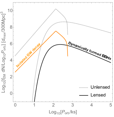
Figure 4: The number of compact-object binaries per log orbital period integrated over a range of binary masses. The orange lines are drawn for a population of compact objects undergoing orbital decay due only to GW radiation (§4.1.1) and are truncated at the maximum orbital periods for which GW decay could merge the pair in a Hubble time (assuming a binary mass ratio of $q=1$). The black lines represent the dynamically formed population of BBHs described in §4.1.2. The gray dotted lines are drawn without taking into account the probability for orbital alignment to cause strong lensing. The probability for a binary to be EM bright is set to $f_{\rm{EM}}=1$ for scaling purposes, in reality this number might be $10^{-5}$, but is uncertain.

$P_{\rm{max}}=10^{2}\rm{ks}$  $\mathcal{D}_{\rm{obs}}=1.0$
Binary type	$\mathcal{R}_{i}\$ [Gpc-3 yr-1]	—Number of Lynx Lensing Candidates—		—Number of Chandra Lensing Candidates—
		Isolated $\left[\frac{\Delta\Omega_{100}}{4\pi}f_{\rm{EM}}/\chi\right]$	Dynamical $\left[\frac{\Delta\Omega_{100}}{4\pi}f_{\rm{EM}}\right]$	Isolated $\left[\frac{\Delta\Omega_{100}}{4\pi}f_{\rm{EM}}/\chi\right]$	Dynamical $\left[\frac{\Delta\Omega_{100}}{4\pi}f_{\rm{EM}}\right]$
BBH	$10-100$	$(10^{6}-10^{7})$	$\sim 10^{5}$	$(10^{3}-10^{4})$	$\sim 10^{2}$
BH-NS	$\leq 600$	$\leq 10^{8}$	–	$\leq 10^{5}$	–
BNS	$100-3800$	$(10^{6}-10^{8})$	–	$(10^{3}-10^{5})$	–

Table 1: The approximate, all-sky number $\mathcal{N}_{\rm{lens}}$ of lensing systems by binary type and formation mechanism multiplied by the fraction $f_{\rm{EM}}$ that emit at or above the Eddington luminosity and by the solid angle $\Delta\Omega_{100}$ of sky observed for at least the duration of the maximum orbital period set to $P_{\rm{max}}=100\rm{ks}$. The quantity $\chi$ is the fraction that will merge within a Hubble time and is only relevant for the "Isolated" category which is tied to the LIGO merger rate. Merger rate ranges are from The LIGO Scientific Collaboration et al. (2018).

4.2 EM emission mechanisms

While there are a number of known X-ray bright accreting compact objects, namely the X-ray binaries (e.g., Charles & Coe, 2003), the only known X-ray bright double compact-object binaries are double neutron star systems identified by the existence of a pulsar in the binary (e.g., Burgay et al., 2003; Chatterjee et al., 2007). As the rate estimate of the previous sub-sections shows, this lack of EM identification of double compact-object binaries may be due to scarcity within the presently observable volume. It is also possible that without a unique identifier of the binary (as exists for the double neutron star system containing a pulsar), double compact-object systems may be confused with single compact-object systems, the point of our work here being to demonstrate self-lensing flares as possible identifiers. A final complication could be the duration for which systems at detectable orbital periods are EM bright, which we discuss presently.

The opportunity to use self-lensing as a tool to study CO binaries exists only if one or both COs emit bright EM radiation, a property we parameterized by the EM duty cycle $f_{\rm{EM}}$ in the previous subsections. One can estimate the EM duty cycle with the simple approximation $f_{\rm{EM}}\sim\tau_{\rm{EM}}/\tau_{\rm merge}$, which relies on an estimate of how long any member of a CO binary can be bright enough for detection and so depends on the distance from the observer and the binary properties, as well as the EM-radiation-generating mechanism itself. Because this is uncertain, and indeed something that an ongoing search for self-lensing flares could constrain, here we simply motivate a few ways that CO binaries could emit near their Eddington luminosities.

While NSs and magnetars can be bright after birth due to magnetically driven spin down power or fallback accretion, they typically only reach sub-Eddington luminosities that render them detectable within our own Milky Way and its satellites. (Kaspi & Beloborodov, 2017; Chatterjee et al., 2000). One exception is the Ultra Luminous X-ray sources that could be super Eddington accretors (Kaaret et al., 2017). However, as the physical nature of these objects is uncertain, we do not attempt to predict their prevalence in binaries or their EM duty cycle here.

BBHs can also be bright for limited times due to fallback accretion (Perna et al., 2014). A fallback disc could contain $M_{d}\equiv q_{d}M$ of material, where M is the total binary mass. If the disc can accrete onto the binary at a fraction $f_{\rm{Edd}}$ of the Eddington rate, $\dot{M}=f_{\rm{Edd}}2.3\times 10^{-8}{M_{\odot}}\rm{yr}^{-1}(M/{M_{\odot}})$, assuming $10\%$ accretion efficiency, then the disc could have a total active lifetime

$$\tau_{\rm{EM}} \approx \frac{q_{d}M}{f_{\rm{Edd}}2.3\times 10^{-8}{M_{\odot}}\rm{yr}^{-1}(M/{M_{\odot}})}$$

$$\approx 4.3\times 10^{5}\rm{yr}\ f^{-1}_{\rm{Edd}}\frac{q_{d}}{10^{-2}},$$

which is the fraction $q_{d}$ of the mass doubling time at rate $f_{\rm{Edd}}$. From this we estimate a duty cycle for EM bright emission $f_{\rm{EM}}\mathrel{\hbox to0.0pt{\lower 4.0pt\hbox{\hskip 1.0pt$\sim$}\hss}\raise 1.0pt\hbox{$<$}}10^{-5}$, assuming that a binary merges in a Hubble time. We note that Perna et al. (2016) and Kimura et al. (2017) explore the possibility of dormant fallback discs being reborn by tidal torques in BBH systems. Specifically, Kimura et al. (2017) find that fallback discs around each BH can be revitalized $\sim 10^{5}$ years before merger, but only with the brightest, super-Eddington stage of accretion happening less than a year before merger.

The formation of the second CO may also occur soon after a common-envelope phase, supplying gas to the CO binary (see Ivanova et al., 2013, for a review). It may be possible for residual accretion to continue to produce EM radiation after the common envelope is ejected.

Another intriguing possibility is accretion onto the CO binary from a stellar companion in an hierarchical triple system. It is increasingly clear that massive stars are born in binaries, and also in hierarchical triples (e.g., Moe & Di Stefano, 2017). The existence of a third star may play an important evolutionary role in allowing the compact binary to form. For example, several studies have invoked secular dynamical interactions (particularly the Kozai-Lidov mechanism) with a wide-orbit companion to shrink the inner orbit so that merger within a Hubble time is possible.

As the third star in an un-evolved star plus CO-binary triple evolves, it will emit winds. In some cases, it may come to fill its Roche lobe. In either case, a fraction of the mass from the outer star will come under the gravitational influence of the stellar remnants in the inner binary. As they fall toward the compact remnants, they can become X-ray bright. The duration of mass transfer is determined by the evolutionary time scale of the outer star. For stars of high mass, one or both components of the inner binary may be X-ray bright for $\sim 10^{5}$ yr, while the time scale is longer, up to $\sim 10^{7}$ yr, for stars of lower mass. An interesting point is that the time to merger evolves as mass is transferred. Changes by more than two orders of magnitude may not be unusual (Di Stefano, 2018). Thus, typical values of the duty cycle $f_{\rm{EM}}$ may be as large as a few percent to unity.

Recently, Samsing et al. (2019), Lopez et al. (2019), and Kremer et al. (2019a) pointed out that in the dynamical formation scenario, BBHs could interact with stars or even planets (Kremer et al., 2019b), allowing both or one BH to become bright via tidal disruptions. Such events could exceed the Eddington luminosity, though for short durations.

While here we have simply sketched a motivation for the possibility of bright EM emission from CO binaries, future work can be carried out to better quantify the possibility for bright (Eddington) and long lived ($\mathrel{\hbox to0.0pt{\lower 4.0pt\hbox{\hskip 1.0pt$\sim$}\hss}\raise 1.0pt\hbox{$>$}}10^{-5}$ of an average merging binary’s lifetime) EM emission caused by a combination of the above possibilities.

5 Discussion

We have shown that binary self-lensing of a bright component of a CO binary by the other could serve as a unique identifier of the progenitors of LIGO and LISA GW sources, namely the stellar-mass-CO inspirals and mergers. We estimate the timescales, magnification, and possible rates of such events. Binaries with periods of order $100$ ks can exhibit repeating self-lensing flares with maximum magnifications ranging from a few to $\times 100$, depending on binary mass. They are detectable within single X-ray observation times, and can merge via GW emission within a Hubble time. Longer orbital period systems (with lensing properties given by systems to the right of the vertical lines in Figure 1) may be more abundant, though detectable as single-flare events that can be followed-up to search for the predicted succeeding flares.

We estimate that, out to a distance to which a Lynx-like future X-ray observatory could see an Eddington limited source, $\sim 10^{7}f_{\rm{EM}}/\chi$ CO binaries, across the entire sky, would have orbital periods of $\mathrel{\hbox to0.0pt{\lower 4.0pt\hbox{\hskip 1.0pt$\sim$}\hss}\raise 1.0pt\hbox{$<$}}100$ ks and be inclined sufficiently to the line of sight to cause strong lensing flares. The same estimate using the flux-sensitivity of Chandra is $\sim 10^{4}f_{\rm{EM}}/\chi$. Here $f_{\rm{EM}}$ parameterizes the unknown duty cycle of CO binaries below a maximum orbital period that have at least one bright component (bolometric luminosity at the Eddington luminosity or greater), and $\chi$ is the fraction of CO binaries at of order $100$ ks orbital periods that will merge rather than stall. For example, $\chi$ could be less than one if gas dynamics slow or prevent merger (Tang et al., 2017; Derdzinski et al., 2019; Muñoz et al., 2019; Moody et al., 2019), or if the binary is broken up during dynamical formation (as happens for the 2-body and 3-body mergers of Samsing & D’Orazio, 2018; D’Orazio & Samsing, 2018).

While the above estimates invoke a steady-state population of GW-driven CO binaries, we also considered a population of BBHs that are driven to merger in GCs via dynamical processes. The total number of lensing candidates predicted via the dynamical channel is consistent with the low-end predictions of the "Isolated" GW-driven channel. It is interesting to note that the two populations have significantly different period distributions that, if probed by a self-lensing population, could differentiate between the two formation scenarios (see also Samsing et al., 2019).

Furthermore, within a given CO-binary formation model, we can constrain the value of $f_{\rm{EM}}/\chi$ by searching for such repeating flares in present X-ray data. Considering the isolated GW-decay model, null detection with Chandra-sensitivity archival data covering $1\%$ of the sky would constrain this quantity to be $f_{\rm{EM}}/\chi\mathrel{\hbox to0.0pt{\lower 4.0pt\hbox{\hskip 1.0pt$\sim$}\hss}\raise 1.0pt\hbox{$<$}}10^{-2}$ and null detections with a similar sky coverage at Lynx-sensitivity would require $f_{\rm{EM}}/\chi\mathrel{\hbox to0.0pt{\lower 4.0pt\hbox{\hskip 1.0pt$\sim$}\hss}\raise 1.0pt\hbox{$<$}}10^{-5}$ (see Eq. 20), which begins to become astrophysically interesting given expectations for certain astrophysical scenarios discussed in §4.2. A wide area X-ray survey with similar sensitivities would improve these constraints by up to two orders of magnitude. If independent measurements of the merging fraction $\chi$ can be made via, e.g., LISA vs. LIGO population analysis, then the EM duty cycle of CO binaries can be constrained.

More interesting would be an observation of a self-lensing event. From such an observation we can learn the orbital period and mass of the binary and its components. For multiple flare detections in a single system, precise phasing of the orbit allowed by flare detection could allow the determination of orbital precession caused by, e.g., surrounding matter or relativistic effects. Identification of multiple binaries via self-lensing would allow us to infer the orbital period distribution of CO binaries at large separations and compare to models such as those plotted in Figure 4. This would open a window into the CO-binary population at a time in their evolution before any GW instrument could detect them. It could also probe the population near formation; this is because $\mathcal{O}(100)$ ks orbital periods, which are ideal for self-lensing detection, are also approximately the orbital periods that delineate merging systems from those that do not merge via GW emission within a Hubble time. For example, equal mass ratio, $3{M_{\odot}}$ BNSs on circular orbits will merger in a Hubble time when starting from $P_{\rm{orb}}\sim 60$ ks while $60{M_{\odot}}$ BBHs will merge in a Hubble time starting from $P_{\rm{orb}}\sim 400$ ks. This suggests that observing BNSs near $100$ ks orbital periods can teach us something about the fraction of BNSs that merge (our parameter $\chi$).

While we have considered specifically Chandra- and Lynx-like instruments in order to observationally ground this study, it is important to consider the interplay between the sky coverage as a function of observation time (setting $\Delta\Omega_{P_{\rm{max}}}$), and the instrument sensitivity (setting $d_{\rm{max}}$). Reading off the scaling of sky coverage and sensitivity from Eq. (20), we can apply our calculation to other X-ray instruments. Compared to Chandra we find,

$$\mathcal{N}_{\rm{lens},\textit{Lynx}} \approx 10^{3}\mathcal{N}_{\rm{lens},\textit{Chandra}}$$

$$\mathcal{N}_{\rm{lens},\textit{Athena}~{}} \approx 30\mathcal{N}_{\rm{lens},\textit{Chandra}}$$

$$\mathcal{N}_{\rm{lens},\textit{Axis}~{}} \approx 30\mathcal{N}_{\rm{lens},\textit{Chandra}}$$ (23)

where, as throughout the rest of this work we have estimated a $100\times$ better sensitivity with Lynx. We have estimated a $10\times$ better sensitivity for Axis and Athena (Nandra et al., 2013; Reynolds & Mushotzky, 2017), with similar end-mission values of $\Delta\Omega_{100}$ for both (while the Athena mission has a larger field of view than Chandra, its mission duration may be shorter). While eRosita is an all-sky survey, it will only observe $\sim 0.01$ percent of the sky for greater than $10$ ks, and with a similar sensitivity to Chandra (Merloni et al., 2012). We also estimate that XMM Newton and SWIFT perform comparably to Chandra for such a task. Ultimately, the combination of data from all of these instruments will allow the most constraining power.

Systems that exhibit periodic self-lensing will also exhibit periodic modulations due to the relativistic Doppler boost. Because, we are considering systems with orbital periods $\mathrel{\hbox to0.0pt{\lower 4.0pt\hbox{\hskip 1.0pt$\sim$}\hss}\raise 1.0pt\hbox{$>$}}1$ ks, and with mass below $\sim 10^{3}{M_{\odot}}$, magnification due to the Doppler boost never becomes as large as in the lensing case. However, the range of binary inclination angles for which moderate Doppler-boost magnification occurs is wider (D’Orazio & Di Stefano, 2018), and so the probability of finding a moderately amplified, periodic, Doppler- boosted system can be higher.

As an example, consider the approximate amplitude of Doppler modulations, $(3-\alpha)v_{\rm{orb}}/c\cos{i}$ for line-sight inclination $i$ and spectral slope $\alpha$. We choose $\alpha=1$ for demonstration. For a $M=10^{3}{M_{\odot}}$ binary, for which Doppler amplification would be the largest, Figure 5 plots the line-of-sight inclination angle dependence of the Doppler-boost magnification as well as lensing magnification for the same binary system. From Figure 5, it clear that lensing magnification greatly dominates over Doppler magnification at small inclination angles, but that the Doppler amplification is still prevalent for a much wider range of inclination angles.

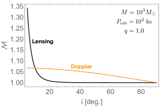
Figure 5: The magnification due to self-lensing (black-solid line) and the relativistic Doppler boost (orange-dashed line) as a function of inclination of the binary to the line of sight. The smallest inclination angle is chosen in order to align the source and the Einstein radius of the lens (strong lensing limit), smaller inclination angles result in lensing amplifications upwards of $100$ for the smallest source sizes (see Figure 2).

To determine for what systems a Doppler-boost detection will be plausible we ask: when will the count rate be high enough for Poisson error bars on the count number to be smaller than the maximum Doppler amplification. We use the unlensed count rate from Eq. (13) and the Doppler amplification motived above to determine the region of binary parameter space where

Poissonerror $$\leq$$ Doppler amplified counts

$$\sqrt{\mathcal{C}_{0}\frac{P_{\rm{orb}}}{2}} \leq \left(\frac{3-\alpha}{c}\frac{1}{1+q}\sqrt{\frac{GM}{a}}\right)\mathcal{C}_{0}\frac{P_{\rm{orb}}}{2}.$$ (24)

The analogous criterion for the lensing case is nearly identical to the count rate criteria depicted by the teal region of Figure 2.

In Figure 6 we plot this region in gray in a plot modeled after Figure 2, but for the Doppler boost instead of lensing magnification. As in Figure 2, the teal region specifies when the system is detectable, except in the Doppler case we use the criteria that one count be observed at the unlensed count rate over half of a binary orbit (rather than requiring one count at the lensed count rate over the duration of the lensing event). Importantly, the criteria for Doppler identification, Eq. (24), is only realized when many counts can be collected, for the most massive, longest period systems. Figure 6 shows that Doppler-boost identification is only viable for binaries with total mass greater than $\sim 10^{3}{M_{\odot}}$. In these cases however, the detection probability can be much higher than for the lensing case (a factor of $10-45\times$ higher for $M=10^{3}{M_{\odot}}$ and $P_{\rm{orb}}=1-100$ ks). Whether or not there are enough BBH systems with mass above $10^{3}{M_{\odot}}$ within a few $\times 100$ Mpc to capitalize on the higher probability of finding such Doppler-boost systems is uncertain.

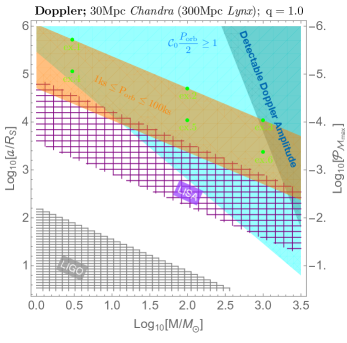
Figure 6: The same as Figure 2, except considering periodic modulation due only to the Doppler boost. Here the teal region labeled $\left<\mathcal{C}\right>P_{\rm{orb}}/2\geq 1$, denotes where the average flux over half of an orbital period results in at least one count for a Chandra-like (Lynx-like) instrument and an Eddington luminosity source at 30 Mpc (300 Mpc). The dark shaded region that overlays a subset of the teal region at high binary masses denotes where there are enough counts to detect the Doppler modulation, i.e., where the Poisson error in the number of counts is smaller than the typical Doppler magnification, Eq. (24).

While self-lensing offers a unique EM signature of CO binaries that may, in their distant future, pass through the LISA band and merge in the LIGO band, it may also offer an EM counterpart to low frequency, near-by LISA sources. This is hinted at by the small overlap of the orange, teal, and hatched purple regions in Figures 2 and 6 and is explored in further detail in Figure 7. Figure 7 plots GW characteristic strain vs. GW frequency, plotting the four-year-LISA (black; SNR=1) and O2 LIGO (grey; SNR=1) sensitivity curves for reference. The shaded purple regions denote the GW strain over the lifetime of inspiralling CO binaries at 10 Mpc (‘+” hatched) and 100 Mpc (‘x’ hatched) in the mass ranges of $3\leq M/{M_{\odot}}\leq 100$ (see D’Orazio & Samsing, 2018, for an explanation of how these are drawn). The orange region of Figures 2 and 6 is also plotted in orange in Figure 7, but in GW frequency space assuming circular orbits. The overlap of orange and purple regions above the LISA sensitivity curve shows that self-lensing EM counterparts to LISA sources are a possibility for the closest and most massive binaries. This could be interesting as a few such sources are predicted to exist (Kremer et al., 2019c).

The shorter orbital period lensing events, below our $1$ ks cut (to the right of the orange region in Figure 7), could still, in principle, be detected. LISA inspirals should be monitored for such periodic EM emission. Lensing events from sources entering the LIGO band are spaced too closely in time and are too short in duration to be discerned with current or near future X-ray telescopes. We note, however, that the microsecond cadence of gamma-ray burst detectors such as Fermi GBM (FERMI-Collaboration, 2015) may allow detection of such events. The detection of an EM chirp from such a lensing signature near merger has been investigated with a dynamical spacetime ray-tracing code by Schnittman et al. (2018).

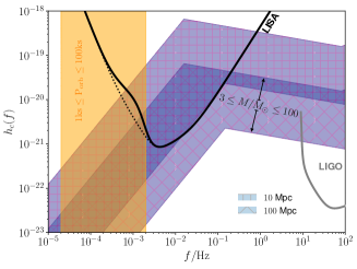
Figure 7: The overlap of the orange region of Figures 2 and 6 with the LISA band (Robson et al., 2019). For reference we have shaded in purple the tracks of characteristic strain vs. GW frequency of CO binaries with masses ranging from $3-100{M_{\odot}}$ at distances of 10 and 100 Mpc as they pass through the LISA band (SNR=1 drawn in black) and the LIGO band (SNR=1 drawn in gray).

6 Conclusions

We conclude with some caveats and prospects for future work.

We have assumed circular binary orbits in our lensing models. Inclusion of eccentricity changes the shape of lensing curves but does not significantly alter the lensing duration or magnification. Eccentric self-lensing is explored in Hu et al. (2019).

Here we have focused on X-ray observations of self-lensing because X-rays naturally emanate from the smallest regions bound to BHs and NSs. However, emission regions at optical and UV wavelengths can also exhibit self-lensing signatures and may benefit from the upcoming and present all-sky time-domain surveys such as the Zwicky Transient Facility (ZTF, Bellm et al., 2019) and The Large Synoptic Survey Telescope (LSST, Ivezic & et al., 2008). That is, optical emission may be more extended and, hence, not as highly magnified as the X-ray emission region, but a much larger volume of space could be surveyed in optical. This should be considered in future work.

Because of their repetition, symmetric pulse shape, and large magnifications, self-lensing flares have high potential for being a uniquely identifiable electromagnetic signature of compact-object binaries. Hence, in optical or in X-ray, these unique signatures should be searched for. Null search results will constrain the merging fraction in combination with the EM-bright lifetime of compact-object binaries, while a detection of self-lensing offers a direct window into their formation and early life.

References

- Abbott et al. (2016a) Abbott B. P., et al., 2016a, Physical Review X, 6, 041015
- Abbott et al. (2016b) Abbott B. P., et al., 2016b, Physical Review Letters, 116, 061102
- Abbott et al. (2016c) Abbott B. P., et al., 2016c, Physical Review Letters, 116, 241103
- Abbott et al. (2017a) Abbott B. P., et al., 2017a, Physical Review Letters, 118, 221101
- Abbott et al. (2017b) Abbott B. P., et al., 2017b, Physical Review Letters, 119, 141101
- Abbott et al. (2017c) Abbott B. P., et al., 2017c, Physical Review Letters, 119, 161101
- Abbott et al. (2017d) Abbott B. P., et al., 2017d, ApJL, 850, L40
- Abbott et al. (2017e) Abbott B. P., et al., 2017e, ApJL, 851, L35
- Amaro-Seoane et al. (2017) Amaro-Seoane P., et al., 2017, preprint, (arXiv:1702.00786)
- Antonini & Perets (2012) Antonini F., Perets H. B., 2012, ApJ, 757, 27
- Antonini et al. (2017) Antonini F., Toonen S., Hamers A. S., 2017, ApJ, 841, 77
- Askar et al. (2017) Askar A., Szkudlarek M., Gondek-Rosińska D., Giersz M., Bulik T., 2017, MNRAS, 464, L36
- Bae et al. (2014) Bae Y.-B., Kim C., Lee H. M., 2014, MNRAS, 440, 2714
- Banerjee et al. (2010) Banerjee S., Baumgardt H., Kroupa P., 2010, MNRAS, 402, 371
- Bartos et al. (2017) Bartos I., Kocsis B., Haiman Z., Márka S., 2017, ApJ, 835, 165
- Belczynski et al. (2016a) Belczynski K., Holz D. E., Bulik T., O’Shaughnessy R., 2016a, Nature, 534, 512
- Belczynski et al. (2016b) Belczynski K., Repetto S., Holz D. E., O’Shaughnessy R., Bulik T., Berti E., Fryer C., Dominik M., 2016b, ApJ, 819, 108
- Bellm et al. (2019) Bellm E. C., et al., 2019, PASP, 131, 018002
- Bird et al. (2016) Bird S., Cholis I., Muñoz J. B., Ali-Haïmoud Y., Kamionkowski M., Kovetz E. D., Raccanelli A., Riess A. G., 2016, Physical Review Letters, 116, 201301
- Burgay et al. (2003) Burgay M., et al., 2003, Nature, 426, 531
- Charles & Coe (2003) Charles P. A., Coe M. J., 2003, arXiv e-prints, pp astro–ph/0308020
- Chatterjee et al. (2000) Chatterjee P., Hernquist L., Narayan R., 2000, ApJ, 534, 373
- Chatterjee et al. (2007) Chatterjee S., Gaensler B. M., Melatos A., Brisken W. F., Stappers B. W., 2007, ApJ, 670, 1301
- Christian & Loeb (2017) Christian P., Loeb A., 2017, MNRAS, 469, 930
- D’Orazio & Di Stefano (2018) D’Orazio D. J., Di Stefano R., 2018, MNRAS, 474, 2975
- D’Orazio & Loeb (2018) D’Orazio D. J., Loeb A., 2018, PRD, 97, 083008
- D’Orazio & Samsing (2018) D’Orazio D. J., Samsing J., 2018, MNRAS, 481, 4775
- D’Orazio et al. (2015) D’Orazio D. J., Haiman Z., Schiminovich D., 2015, Nature, 525, 351
- Derdzinski et al. (2019) Derdzinski A. M., D’Orazio D., Duffell P., Haiman Z., MacFadyen A., 2019, MNRAS, 486, 2754
- Di Stefano (2018) Di Stefano R., 2018, arXiv e-prints, p. arXiv:1805.09338
- Dominik et al. (2012) Dominik M., Belczynski K., Fryer C., Holz D. E., Berti E., Bulik T., Mandel I., O’Shaughnessy R., 2012, ApJ, 759, 52
- Dominik et al. (2013) Dominik M., Belczynski K., Fryer C., Holz D. E., Berti E., Bulik T., Mandel I., O’Shaughnessy R., 2013, ApJ, 779, 72
- Dominik et al. (2015) Dominik M., et al., 2015, ApJ, 806, 263
- Evans et al. (2010) Evans I. N., et al., 2010, ApJS, 189, 37
- FERMI-Collaboration (2015) FERMI-Collaboration 2015, FERMI GBM charecteristics, http://gammaray.msfc.nasa.gov/gbm/
- Fabbiano (2019) Fabbiano G., 2019, arXiv e-prints, p. arXiv:1903.01970
- Fishbach et al. (2017) Fishbach M., Holz D. E., Farr B., 2017, ApJL, 840, L24
- Fryer et al. (2001) Fryer C. L., Woosley S. E., Heger A., 2001, ApJ, 550, 372
- Gaskin et al. (2018) Gaskin J. A., et al., 2018, in Space Telescopes and Instrumentation 2018: Ultraviolet to Gamma Ray. p. 106990N, doi:10.1117/12.2314149
- Gerosa & Berti (2017) Gerosa D., Berti E., 2017, PRD, 95, 124046
- Gerosa et al. (2013) Gerosa D., Kesden M., Berti E., O’Shaughnessy R., Sperhake U., 2013, PRD, 87, 104028
- Gerosa et al. (2015) Gerosa D., Kesden M., Sperhake U., Berti E., O’Shaughnessy R., 2015, PRD, 92, 064016
- Gerosa et al. (2019) Gerosa D., Ma S., Wong K. W. K., Berti E., O’Shaughnessy R., Chen Y., Belczynski K., 2019, PRD, 99, 103004
- Harris (2010) Harris W. E., 2010, arXiv e-prints, p. arXiv:1012.3224
- Heggie & Hut (2003) Heggie D., Hut P., 2003, The Gravitational Million-Body Problem: A Multidisciplinary Approach to Star Cluster Dynamics
- Hu et al. (2019) Hu B. X., D’Orazio D. J., Haiman Z., Smith K. L., Snios B., Charisi M., Di Stefano R., 2019, arXiv e-prints, p. arXiv:1910.05348
- Ivanova et al. (2013) Ivanova N., et al., 2013, A&ARv, 21, 59
- Ivezic & et al. (2008) Ivezic Z., et al. 2008, preprint, (arXiv:0805.2366)
- Kaaret et al. (2017) Kaaret P., Feng H., Roberts T. P., 2017, ARA&A, 55, 303
- Kaspi & Beloborodov (2017) Kaspi V. M., Beloborodov A. M., 2017, ARA&A, 55, 261
- Kesden et al. (2015) Kesden M., Gerosa D., O’Shaughnessy R., Berti E., Sperhake U., 2015, Physical Review Letters, 114, 081103
- Kimura et al. (2017) Kimura S. S., Takahashi S. Z., Toma K., 2017, MNRAS, 465, 4406
- Kremer et al. (2019a) Kremer K., Lu W., Rodriguez C. L., Lachat M., Rasio F., 2019a, arXiv e-prints, p. arXiv:1904.06353
- Kremer et al. (2019b) Kremer K., D’Orazio D. J., Samsing J., Chatterjee S., Rasio F. A., 2019b, arXiv e-prints, p. arXiv:1908.06978
- Kremer et al. (2019c) Kremer K., et al., 2019c, PRD, 99, 063003
- Kremer et al. (2019d) Kremer K., Chatterjee S., Ye C. S., Rodriguez C. L., Rasio F. A., 2019d, ApJ, 871, 38
- Liu & Lai (2017) Liu B., Lai D., 2017, ApJL, 846, L11
- Loeb (2016) Loeb A., 2016, ApJL, 819, L21
- Lopez et al. (2019) Lopez Martin J., Batta A., Ramirez-Ruiz E., Martinez I., Samsing J., 2019, ApJ, 877, 56
- Mandel & de Mink (2016) Mandel I., de Mink S. E., 2016, MNRAS, 458, 2634
- Marchant et al. (2016) Marchant P., Langer N., Podsiadlowski P., Tauris T. M., Moriya T. J., 2016, A&A, 588, A50
- McKernan et al. (2018) McKernan B., et al., 2018, ApJ, 866, 66
- Merloni et al. (2012) Merloni A., et al., 2012, arXiv e-prints, p. arXiv:1209.3114
- Moe & Di Stefano (2017) Moe M., Di Stefano R., 2017, ApJS, 230, 15
- Montero-Dorta & Prada (2009) Montero-Dorta A. D., Prada F., 2009, MNRAS, 399, 1106
- Moody et al. (2019) Moody M. S. L., Shi J.-M., Stone J. M., 2019, ApJ, 875, 66
- Muñoz et al. (2019) Muñoz D. J., Miranda R., Lai D., 2019, ApJ, 871, 84
- Nandra et al. (2013) Nandra K., et al., 2013, arXiv e-prints, p. arXiv:1306.2307
- Naoz (2016) Naoz S., 2016, ARA&A, 54, 441
- Park et al. (2017) Park D., Kim C., Lee H. M., Bae Y.-B., Belczynski K., 2017, MNRAS, 469, 4665
- Perna et al. (2014) Perna R., Duffell P., Cantiello M., MacFadyen A. I., 2014, ApJ, 781, 119
- Perna et al. (2016) Perna R., Lazzati D., Giacomazzo B., 2016, ApJ, 821, L18
- Portegies Zwart & McMillan (2000) Portegies Zwart S. F., McMillan S. L. W., 2000, ApJL, 528, L17
- Randall & Xianyu (2018) Randall L., Xianyu Z.-Z., 2018, ApJ, 864, 134
- Reynolds & Mushotzky (2017) Reynolds C. S., Mushotzky R., 2017, in AAS/High Energy Astrophysics Division #16. AAS/High Energy Astrophysics Division. p. 103.23
- Robson et al. (2019) Robson T., Cornish N. J., Liug C., 2019, Classical and Quantum Gravity, 36, 105011
- Rodriguez & Antonini (2018) Rodriguez C. L., Antonini F., 2018, ApJ, 863, 7
- Rodriguez & Loeb (2018) Rodriguez C. L., Loeb A., 2018, ApJL, 866, L5
- Rodriguez et al. (2015) Rodriguez C. L., Morscher M., Pattabiraman B., Chatterjee S., Haster C.-J., Rasio F. A., 2015, Physical Review Letters, 115, 051101
- Rodriguez et al. (2016a) Rodriguez C. L., Chatterjee S., Rasio F. A., 2016a, PRD, 93, 084029
- Rodriguez et al. (2016b) Rodriguez C. L., Zevin M., Pankow C., Kalogera V., Rasio F. A., 2016b, ApJL, 832, L2
- Rodriguez et al. (2018a) Rodriguez C. L., Amaro-Seoane P., Chatterjee S., Kremer K., Rasio F. A., Samsing J., Ye C. S., Zevin M., 2018a, PRD, 98, 123005
- Rodriguez et al. (2018b) Rodriguez C. L., Amaro-Seoane P., Chatterjee S., Rasio F. A., 2018b, Physical Review Letters, 120, 151101
- Samsing & D’Orazio (2018) Samsing J., D’Orazio D. J., 2018, MNRAS, 481, 5445
- Samsing et al. (2018) Samsing J., D’Orazio D. J., Askar A., Giersz M., 2018, arXiv e-prints, p. arXiv:1802.08654
- Samsing et al. (2019) Samsing J., Venumadhav T., Dai L., Martinez I., Batta A., Lopez Martin J., Ramirez-Ruiz E., Kremer K., 2019, arXiv e-prints, p. arXiv:1901.02889
- Schnittman et al. (2018) Schnittman J. D., Dal Canton T., Camp J., Tsang D., Kelly B. J., 2018, ApJ, 853, 123
- Silsbee & Tremaine (2017) Silsbee K., Tremaine S., 2017, ApJ, 836, 39
- Stone et al. (2017) Stone N. C., Metzger B. D., Haiman Z., 2017, MNRAS, 464, 946
- Tang et al. (2017) Tang Y., MacFadyen A., Haiman Z., 2017, MNRAS, 469, 4258
- Tanikawa (2013) Tanikawa A., 2013, MNRAS, 435, 1358
- The LIGO Scientific Collaboration et al. (2018) The LIGO Scientific Collaboration et al., 2018, arXiv e-prints, p. arXiv:1811.12907
- Voss & Tauris (2003) Voss R., Tauris T. M., 2003, MNRAS, 342, 1169
- Yang et al. (2015) Yang Q.-X., Xie F.-G., Yuan F., Zdziarski A. A., Gierliński M., Ho L. C., Yu Z., 2015, MNRAS, 447, 1692
- Zhang et al. (2019) Zhang F., Shao L., Zhu W., 2019, ApJ, 877, 87
- de Mink & Mandel (2016) de Mink S. E., Mandel I., 2016, MNRAS, 460, 3545