Chaining Meets Chain Rule:
Multilevel Entropic Regularization and Training of Neural Nets

Abstract

We derive generalization and excess risk bounds for neural nets using a family of complexity measures based on a multilevel relative entropy. The bounds are obtained by introducing the notion of generated hierarchical coverings of neural nets and by using the technique of chaining mutual information introduced in Asadi et al. NeurIPS’18. The resulting bounds are algorithm-dependent and exploit the multilevel structure of neural nets. This, in turn, leads to an empirical risk minimization problem with a multilevel entropic regularization. The minimization problem is resolved by introducing a multi-scale generalization of the celebrated Gibbs posterior distribution, proving that the derived distribution achieves the unique minimum. This leads to a new training procedure for neural nets with performance guarantees, which exploits the chain rule of relative entropy rather than the chain rule of derivatives (as in backpropagation). To obtain an efficient implementation of the latter, we further develop a multilevel Metropolis algorithm simulating the multi-scale Gibbs distribution, with an experiment for a two-layer neural net on the MNIST data set.

1 Introduction

We introduce a family of complexity measures for the hypotheses of neural nets, based on a multilevel relative entropy. These complexity measures take into account the multilevel structure of neural nets, as opposed to the classical relative entropy (KL-divergence) term derived from PAC-Bayesian bounds [1] or mutual information bounds [2, 3]. We derive these complexity measures by combining the technique of chaining mutual information (CMI) [4], an algorithm-dependent extension of the classical chaining technique paired with the mutual information bound [2], with the multilevel architecture of neural nets. It is observed in this paper that if a neural net is regularized in a multilevel manner as defined in Section 4, then one can readily construct hierarchical coverings with controlled diameters for its hypothesis set, and exploit this to obtain new multi-scale and algorithm-dependent generalization bounds and, in turn, new regularizers and training algorithms. The effect of such multilevel regularizations on the representation ability of neural nets has also been recently studied in [5, 6] for the special case where layers are nearly-identity functions as for ResNets [7]. Here, we demonstrate the advantage of multilevel architectures by showing how one can obtain accessible hierarchical coverings for their hypothesis sets, introducing the notion of architecture-generated coverings in Section 3. Then we derive our generalization bound for arbitrary-depth feedforward neural nets via applying the CMI technique directly on their hierarchical sequence of generated coverings. Although such a sequence of coverings may not give the tightest possible generalization bound, it has the major advantage of being easily accessible, and hence can be exploited in devising multilevel training algorithms. Designing training algorithms based on hierarchical coverings of hypothesis sets has first been studied in [8], and has recently regained traction in e.g. [9, 10], all in the context of online learning and prediction of individual sequences. With such approaches, hierarchical coverings are no longer viewed merely as methods of proof for generalization bounds: they further allow for algorithms achieving low statistical error.

In our case, the derived generalization bound puts forward a multilevel relative entropy term (see Definition 1). We then turn to minimizing the empirical error with this induced regularization, called here the multilevel entropic regularization. Interestingly, we can solve this minimization problem exactly, obtaining a multi-scale generalization of the celebrated Gibbs posterior distribution; see Sections 5 and 6. The target distribution is obtained in a backwards manner by successive marginalization and tilting of distributions, as described in the Marginalize-Tilt algorithm introduced in Section 6. Unlike the classical Gibbs distribution, its multi-scale counter-part possesses a temperature vector rather than a global temperature. We then present a multilevel training algorithm by simulating our target distribution via a multilevel Metropolis algorithm introduced for a two layer net in Section 7. In contrast to the celebrated back-propagation algorithm which exploits the chain rule of derivatives, our target distribution and its simulated version are derived from the chain rule of relative entropy, and take into account the interactions between different scales of the hypothesis sets of neural nets corresponding to different depths.

This paper introduces the new concepts and main results behind this alternative approach to training neural nets. Many directions emerge from this approach, in particular for its applicability. It is worth noting that Markov chain Monte Carlo (MCMC) methods are known to often better cope with non-convexity issues than gradient descent approaches, since they are able to backtrack from local minima [11]. Furthermore, in contrast to gradient descent, MCMC methods take into account parameter uncertainty that helps preventing overfitting [12]. However, compared to gradient based methods, these methods are typically computationally more demanding.

Further related literature

Information-theoretic approaches to statistical learning have been studied in the PAC-Bayesian theory; see [1, 13, 14] and references therein, and via the recent mutual information bound in e.g. [2, 3, 15, 16, 17, 18, 19]. Deriving generalization bounds for neural nets, based on the PAC-Bayesian theory, has been the focus of recent studies such as [20, 21, 22, 23]. The statistical properties of the Gibbs posterior distribution, also known as the Boltzmann distribution, or the exponential weights distribution in e.g. [24], have been studied in e.g. [25, 26, 27, 3, 15] via an information-theoretic viewpoint. Applications of the Gibbs distribution in devising and analyzing training algorithms have been the focus of recent studies such as [28, 29, 30]. Tilted distributions in unsupervised and semi-supervised statistical learning problems has also been studied in [31] in the context of community detection. For results on applying MCMC methods to large data sets, see [32] and references therein.

Notation

In this paper, all logarithms are in natural base and all information-theoretic measures are in nats. Let $\imath_{P\|Q}$, $D(P\|Q)$ and $D_{\lambda}(P\|Q)$ denote the relative information, the relative entropy, and the Rényi divergence of order $\lambda$ between probability measures $P$ and $Q$, and let $D(P_{Y|X}\|Q_{Y|X}|P_{X})\triangleq\int D(P_{Y|X=\omega}\|Q_{Y|X=\omega})\mathrm{d}P_{X}(\omega)$ denote conditional relative entropy (see Appendix A for precise definitions). In the framework of supervised statistical learning, $\mathcal{X}$ denotes the instances domain, $\mathcal{Y}$ is the labels domain, $\mathsf{Z}=\mathcal{X}\times\mathcal{Y}$ denotes the examples domain and $\mathcal{H}=\{h_{w}:w\in\mathcal{W}\}$ is the hypothesis set, where the hypotheses are indexed by an index set $\mathcal{W}$. Let $\ell:\mathcal{W}\times\mathsf{Z}\to\mathbb{R}^{+}$ be the loss function. A learning algorithm receives the training set $S=(Z_{1},Z_{2},...,Z_{n})$ of $n$ examples with i.i.d. random elements drawn from $\mathsf{Z}$ with an unknown distribution $\mu$. Then it picks an element $h_{W}\in\mathcal{H}$ as the output hypothesis according to a random transformation $P_{W|S}$. For any $w\in\mathcal{W}$, let $L_{\mu}(w)\triangleq\mathbb{E}[\ell(w,Z)]$ denote the statistical (or population) risk of hypothesis $h_{w}$, where $\leavevmode\nobreak\ Z\sim\mu$. For a given training set $S$, the empirical risk of hypothesis $h_{w}$ is defined as $L_{S}(w)\triangleq\frac{1}{n}\sum_{i=1}^{n}\ell(w,Z_{i}),$ and the generalization error of hypothesis $h_{w}$ (dependent on the training set) is defined as $\mathrm{gen}(w)\triangleq L_{\mu}(w)-L_{S}(w).$ Averaging with respect to the joint distribution $P_{S,W}=\mu^{\otimes n}P_{W|S}$, we denote the expected generalization error by $\mathrm{gen}(\mu,P_{W|S})\triangleq\mathbb{E}[\mathrm{gen}(W)],$ and the average statistical risk by $\mathrm{risk}(\mu,P_{W|S})\triangleq\mathbb{E}[L_{\mu}(W)].$ Throughout the paper, $\|A\|_{2}$ denotes the spectral norm of matrix $A$ and $|b|_{2}$ denotes the Euclidean norm of vector $b$. Let $\delta_{w}$ denote the Dirac measure centered at $w$.

2 Preliminary: The CMI technique

Chaining, originated from the work of Kolmogorov and Dudley, is a powerful technique in high dimensional probability for bounding the expected suprema of random processes while taking into account the dependencies between their random variables in a multi-scale manner. Here we emphasize the core idea of the chaining technique: performing refined approximations by using a telescoping sum, named as the chaining sum. If $\{X_{t}\}_{t\in T}$ is a random process, then for any $t\in T$ one can write

$$X_{t}=X_{\pi_{1}(t)}+\left(X_{\pi_{2}(t)}-X_{\pi_{1}(t)}\right)+\dots+\left(X_{\pi_{d}(t)}-X_{\pi_{d-1}(t)}\right)+\left(X_{t}-X_{\pi_{d}(t)}\right),$$

where $\pi_{1}(t),\pi_{2}(t),\dots,\pi_{d}(t)$ are finer and finer approximations of the index $t$. Each of the differences $X_{\pi_{k}(t)}-X_{\pi_{k-1}(t)}$, $k=1,2,\dots,d$, is called a link of the chaining sum. Informally speaking, if the approximations $\pi_{k}(t)$, $k=1,2,\dots,d$, are close enough to each other and $\pi_{d}(t)$ is close to $t$, then, in many important applications, controlling the expected supremum of each of the links with union bounds and summing them up will give a much tighter bound than bounding the supremum of $X_{t}$ upfront with a union bound. For instance, the approximations may be the projections of $t$ on an increasing sequence of partitions of $T$. For more information, see [33, 34, 35] and references therein.

The technique of chaining mutual information, recently introduced in [4], can be interpreted as an algorithm-dependent version of the above, extending a result of Fernique [36] by taking into account such dependencies. In brief, [4] asserts that one can replace the metric entropy in chaining with the mutual information between the input and the discretized output, to obtain an upper bound on the expected bias $\mathbb{E}[X_{W}]$ of an algorithm which selects its output from a random process $\{X_{t}\}_{t\in T}$. By writing the chaining sum with random index $W$ and after taking expectations, we obtain:

$$\mathbb{E}\left[X_{W}\right]=\mathbb{E}\left[X_{\pi_{1}(W)}\right]+\mathbb{E}\left[X_{\pi_{2}(W)}-X_{\pi_{1}(W)}\right]+\dots+\mathbb{E}\left[X_{W}-X_{\pi_{d}(W)}\right].$$ (1)

With this technique, rather than bounding $\mathbb{E}\left[X_{W}\right]$ with a single mutual information term such as in [2, 3], one bounds each link $\mathbb{E}\left[X_{\pi_{k}(W)}-X_{\pi_{k-1}(W)}\right]$, $k=1,2,\dots,d$, and then sums them up.

In this paper, first we note that unlike the classical chaining method in which we require finite size partitions whose cardinalities appear in the bounds, that requirement is unnecessary for the CMI technique. Therefore one may use a hierarchical sequence of coverings of the index set which includes covers of possibly uncountably infinite size. This fact will be useful for analyzing neural nets with continuous weight values in the next sections. For details, see Appendix B.

The second important contribution is to design the coverings to meet the multilayer structure of neural nets. In the classical chaining and the CMI in [4], these are applied on an arbitrary infinite sequence of $2^{-k}$-partitions. In this paper, we take a different approach and use the hierarchical sequences of generated coverings associated with multilevel architectures, as defined in the next section.

3 Multilevel architectures and their generated coverings

Assume that in a statistical learning problem, the hypothesis set $\mathcal{H}$ consists of multilevel functions, i.e., the index set $\mathcal{W}=\mathcal{W}_{1}\times\cdots\times\mathcal{W}_{d}$ consists of elements $w\in\mathcal{W}$ representable with $d\geq 2$ components as $w=(\mathbf{W}_{1},\dots,\mathbf{W}_{d})$. Examples for neural nets can be: 1. When the components are the layers. 2. When the components are stacks of layers plus skip connections, such as in ResNets [7]. For all $1\leq k\leq d$, let $\mathcal{G}_{k}$ be the exact covering of $\mathcal{W}$ determined by all possible values of the first $k$ components, i.e. any two indices are in the same set if and only their first $k$ components match:

$$\mathcal{G}_{k}\triangleq\left\{\{\mathbf{W}_{1}\}\times\cdots\times\{\mathbf{W}_{k}\}\times\mathcal{W}_{k+1}\times\cdots\times\mathcal{W}_{d}:(\mathbf{W}_{1},\dots,\mathbf{W}_{k})\in\mathcal{W}_{1}\times\cdots\times\mathcal{W}_{k}\right\}.$$

Notice that $\{\mathcal{G}_{k}\}_{k=1}^{d}$ is a hierarchical sequence of exact coverings of the index set $\mathcal{W}$, and the projection set of any $w\in\mathcal{W}$ in $\mathcal{G}_{k}$, i.e., the unique set in $\mathcal{G}_{k}$ which includes $w$, is determined only by the values of the first $k$ components of $w$. We call $\{\mathcal{G}_{k}\}_{k=1}^{d}$ the hierarchical sequence of generated coverings of the index set $\mathcal{W}$, and will use the CMI technique on this sequence in the next sections.

Remark 1.

The notion of generated coverings of $\mathcal{W}$ is akin in nature to the notion of generated filtrations of random processes in probability theory (for a definition, see e.g. [38, p. 171]) and applying the CMI technique on this sequence is akin to the martingale method.

We provide the following simple yet useful example by revisiting Example 1 of [4]:

Example 1.

Consider a canonical Gaussian process $X_{t}\triangleq\langle t,G^{n}\rangle,t\in T$ where $n=2$, $G^{2}=(G_{1},G_{2})$ has independent standard normal components and $T\triangleq\{t\in\mathbb{R}^{2}:|t|_{2}=1\}$. The process $\{X_{t}\}_{t\in T}$ can also be expressed according to the phase of each point $t\in T$, i.e. the unique number $\phi\in[0,2\pi)$ such that $t=(\sin\phi,\cos\phi)$. Assume that the indices are in the phase form and define the following dyadic sequence of partitions of $T$: For all integers $k\geq 1$,

$$\mathcal{P}_{k}\triangleq\left\{\left[0,\frac{2\pi}{2^{k}}\right),\left[\frac{2\pi}{2^{k}},2\times\frac{2\pi}{2^{k}}\right),...,\left[\left(2^{k}-1\right)\frac{2\pi}{2^{k}},2\pi\right)\right\};$$

see Figure 1.

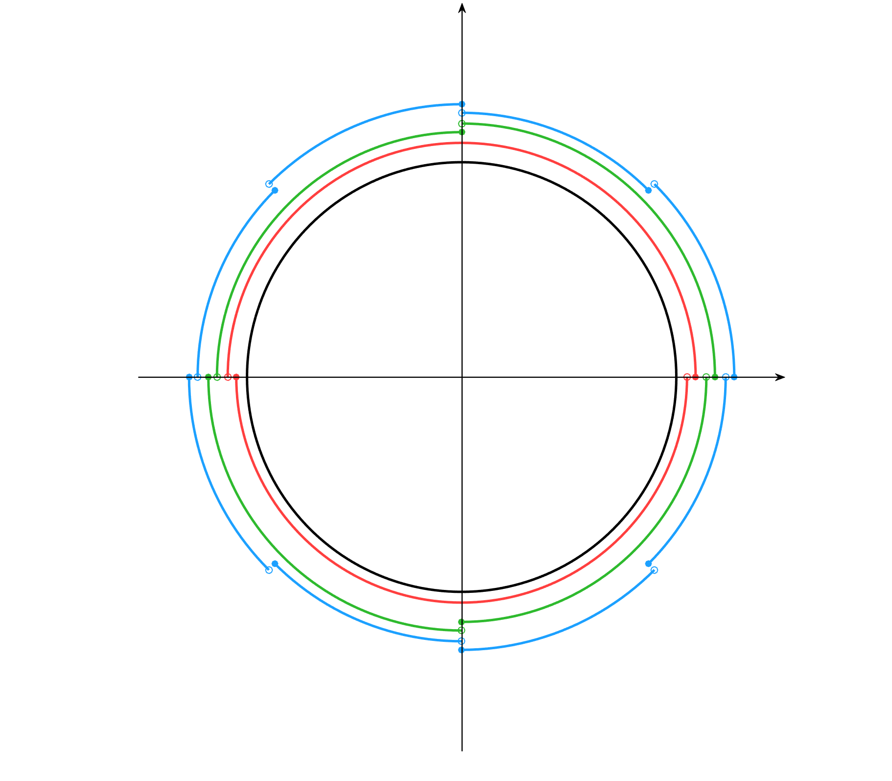
Figure 1: Dyadic sequence of partitions of $T$

Can $T$ and the sequence $\{\mathcal{P}_{k}\}_{k=1}^{\infty}$ be related to the hypothesis set of a multilevel architecture and its generated coverings? For all integers $i\geq 1$, let $\mathcal{W}_{i}\triangleq\left\{\begin{bmatrix}\cos\theta&-\sin\theta\\ \sin\theta&\cos\theta\end{bmatrix}\middle|\theta\in\left\{-\frac{\pi}{2^{i}},\frac{\pi}{2^{i}}\right\}\right\}.$ Notice that for each $t=[t_{1},t_{2}]\in T$, one can write

$$X_{t} =\begin{bmatrix}t_{1}&t_{2}\end{bmatrix}G^{2}$$

$$=\begin{bmatrix}1&0\end{bmatrix}\left(\cdots W_{2}W_{1}\right)G^{2},$$

where each $W_{i}\in\mathcal{W}_{i}$ is uniquely determined by $t$. Fixing the values of $W_{1},\dots,W_{k}$ and allowing the rest of the matrices to take arbitrary values in their corresponding $\mathcal{W}_{i}$ gives one of the elements of $\mathcal{P}_{k}$. Therefore, the sequence of generated coverings associated with the index set of the infinite-depth linear neural net

$$f_{W}(G^{2})=\begin{bmatrix}1&0\end{bmatrix}\left(\cdots W_{2}W_{1}\right)G^{2}$$

is $\{\mathcal{P}_{k}\}_{k=1}^{\infty}$.

4 Multilevel regularization

The purpose of multilevel regularization is to control the diameters of the generated coverings and the links of its corresponding chaining sum. Consider a $d$ layer feed-forward neural net with parameters $w\triangleq(\mathbf{W}_{1},\mathbf{W}_{2},\dots,\mathbf{W}_{d})\in\mathcal{W},$ where for all $1\leq k\leq d$, $\mathbf{W}_{k}\in\mathbb{R}^{\delta_{k}\times\delta_{k-1}}$ is a matrix between hidden layers $k-1$ and $k$. Let $\phi$ denote any non-linearity which is $1$-Lipschitz and satisfies $\phi(0)=0$, such as the entry-wise ReLU activation function, and let $\phi_{o}$ either be the soft-max function, or the identity function. For a given $R>0$, assume that the instances domain is $\mathcal{X}\triangleq\{x^{m}\in\mathbb{R}^{m}:|x^{m}|_{2}\leq R\}$. The feed-forward neural net with parameters $w$ is a function $h_{w}:\mathcal{X}\to\mathbb{R}^{\delta_{d}}$ defined as $h_{w}(x^{m})\triangleq\phi_{o}(\mathbf{W}_{d}(\phi(\cdots\phi(\mathbf{W}_{1}(x^{m}))\cdots))).$ For all $1\leq k\leq d$, let $M_{k}\in\mathbb{R}^{\delta_{k}\times\delta_{k-1}}$ be a fixed matrix such that $\|M_{k}\|_{2}>0$, and for $\alpha_{k}>0$, define the following set of matrices:

$$\mathcal{W}_{k}\triangleq\{\mathbf{W}\in\mathbb{R}^{\delta_{k+1}\times\delta_{k}}:\|\mathbf{W}-M_{k}\|_{2}\leq\alpha_{k}\|M_{k}\|_{2}\}.$$ (2)

We assume that the domain of $\mathbf{W}_{k}$ is restricted to $\mathcal{W}_{k}$. We are regularizing $\mathbf{W}_{k}$ with $M_{k}$ and $\alpha_{k}$, for all $1\leq k\leq d$, to constrain the links of the chaining sum , as we will see in Lemma 1. We name $M_{k}$ and $\alpha_{k}$ as the reference and radius of $\mathcal{W}_{k}$, respectively. A common example used in practice is to let the references be identity matrices, such as for residual nets (see e.g. [5, 6, 39]). For instance, for the linear neural net in Example 1, we can take $M_{k}=I_{2\times 2}$ and $\alpha_{k}=\pi 2^{-k}$, for all $k\geq 1$.

We define the projection of $w$ on the generated covering $\mathcal{G}_{k}$ as $(\mathbf{W}_{1},\dots,\mathbf{W}_{k},M_{k+1},\dots,M_{d})$. Let $M\triangleq\prod_{j=1}^{d}\|M_{j}\|_{2}$.

Lemma 1.

Let $1\leq k\leq d$. Assume that $w_{1}=(\mathbf{W}_{1},\dots,\mathbf{W}_{k-1},\mathbf{W}_{k},M_{k+1},\dots,M_{d})$ and $w_{2}=(\mathbf{W}_{1},\dots,\mathbf{W}_{k-1},M_{k},M_{k+1},\dots,M_{d})$. Then, for all $x^{m}\in\mathcal{X}$,

$$|h_{w_{1}}(x^{m})-h_{w_{2}}(x^{m})|_{2}\leq\alpha_{k}\exp\left(\sum_{i=1}^{k-1}\alpha_{i}\right)M|x^{m}|_{2}.$$

For a proof, see Appendix C.

Notice that for any $w\in\mathcal{W}$ and any $x^{m}\in\mathcal{X}$, if $\phi_{o}$ is the soft-max function, then $|h_{w}(x^{m})|_{2}\leq 1$, and if $\phi_{o}$ is the identity function, then from (2) and the triangle inequality, we derive $|h_{w}(x^{m})|_{2}\leq\exp\left(\sum_{i=1}^{d}\alpha_{i}\right)MR$. Let the loss function $\ell$ be chosen such that there exists $L>0$ for which for any $w_{1},w_{2}\in\mathcal{W}$ and any $z=(x^{m},y)\in\mathsf{Z}$ we have $|\ell(w_{1},z)-\ell(w_{2},z)|\leq L|h_{w_{1}}(x^{m})-h_{w_{2}}(x^{m})|_{2}$ . A commonly used example is the squared $\ell_{2}$ loss i.e. for the net with parameters $w$ and for any example $z=(x^{m},y)\in\mathsf{Z}$, define $\ell(w,z)\triangleq|h_{w}(x^{m})-y|_{2}^{2}$. For classification problems, assume that the labels $y$ are one-hot vectors, otherwise, let $|y|_{2}\leq 1$. Note that for this loss function, if $\phi_{o}$ is the soft-max function, then one can assume $L=4$, and if $\phi_{o}$ is the identity function, then one can take $L=2+2\exp\left(\sum_{i=1}^{d}\alpha_{i}\right)MR$.

5 Generalization and excess risk bounds

For all $1\leq k\leq d$, let $W_{k}$ denote a random matrix and define $\mathrm{gen}(W_{1},\dots,W_{k})\triangleq\mathrm{gen}(\left[W_{1},\dots,W_{k},M_{k+1},\dots,M_{d}\right])$ and $\beta_{k}\triangleq\alpha_{k}\exp\left(\sum_{i=1}^{k-1}\alpha_{i}\right).$ We can now state the following multi-scale and algorithm-dependent generalization bound derived from the CMI technique, in which mutual informations between the training set $S$ and the first $k$ layers appear:

Theorem 1.

Given the assumptions in the previous section, we have

$$\mathrm{gen}(\mu,P_{W|S})\leq\frac{LMR\sqrt{2}}{\sqrt{n}}\sum_{k=1}^{d}\beta_{k}\sqrt{I(S;W_{1},\dots,W_{k})}.$$ (3)

Proof outline. According to (1), one can write the chaining sum with respect to the sequence of generated coverings as

$$\mathrm{gen}(\mu,P_{W|S})=\mathbb{E}[\mathrm{gen}(W)] =\mathbb{E}[\mathrm{gen}(W_{1})]+\mathbb{E}[\mathrm{gen}(W_{1},W_{2})-\mathrm{gen}(W_{1})]+\dots$$

$$\quad+\mathbb{E}[\mathrm{gen}(W)-\mathrm{gen}(W_{1},\dots,W_{d-1})],$$

while, based on Lemma 1, observe that for all $1\leq k\leq d$,

$$\mathbb{E}[\mathrm{gen}(W_{1},\dots,W_{k})-\mathrm{gen}(W_{1},\dots,W_{k-1})]\leq\frac{LMR\sqrt{2}\beta_{k}}{\sqrt{n}}\sqrt{I(S;W_{1},\dots,W_{k})}.$$

For a complete proof, see Appendix C.

Notice that we can rewrite (3) as

$$\mathrm{risk}\left(\mu,P_{W|S}\right)=\mathbb{E}[L_{\mu}(W)]\leq\mathbb{E}[L_{S}(W)]+\frac{C}{\sqrt{n}}\sum_{k=1}^{d}\beta_{k}\sqrt{I(S;W_{1},\dots,W_{k})},$$ (4)

where $C\triangleq LMR\sqrt{2}$. The goal in statistical learning is to find an algorithm $P_{W|S}$ which minimizes $\mathrm{risk}\left(\mu,P_{W|S}\right)=\mathbb{E}[L_{\mu}(W)].$ To that end, we derive an upper bound on $\mathbb{E}[L_{\mu}(W)]$ from inequality (4) whose minimization over $P_{W|S}$ is algorithmically feasible. If for each $k=1,2,\dots,d$, we define $Q^{(k)}_{W_{1}\dots W_{k}}$ to be a fixed distribution on $\mathcal{W}_{1}\times\cdots\times\mathcal{W}_{k}$ that does not depend on the training set $S$, which we name as prior distribution, then from (4) we deduce

$$\mathrm{risk}\left(\mu,P_{W|S}\right) \leq\mathbb{E}[L_{S}(W)]+\frac{C}{\sqrt{n}}\sum_{k=1}^{d}\beta_{k}\left(\gamma_{k}I(S;W_{1},\dots,W_{k})+\frac{1}{4\gamma_{k}}\right)$$ (5)

$$\leq\mathbb{E}[L_{S}(W)]+\frac{C}{\sqrt{n}}\sum_{k=1}^{d}\beta_{k}\left(\gamma_{k}D\left(P_{W_{1}\dots W_{k}|S}\middle\|Q^{(k)}_{W_{1}\dots W_{k}}\middle|P_{S}\right)+\frac{1}{4\gamma_{k}}\right),$$ (6)

where (5) follows from the inequality $\sqrt{x}\leq cx+\frac{1}{4c}$ for all $x,c>0$, which is upper bounding the concave function $\sqrt{x}$ with a tangent line, and (6) follows from the crucial difference decomposition of mutual information: $I(X;Y)=D(P_{Y|X}\|Q_{Y}|P_{X})-D(P_{Y}\|Q_{Y})$; see Lemma 4 in Appendix A. Given fixed parameters $\gamma_{k}$, $k=1,2,\dots,d$, and for any fixed $n$, let $P^{\star}_{W|S}$ be the conditional distribution which minimizes the right side of (6), i.e.

$$P^{\star}_{W|S}\triangleq\operatorname*{arg\,min}_{P_{W|S}}\left\{\mathbb{E}[L_{S}(W)]+\frac{C}{\sqrt{n}}\sum_{k=1}^{d}\beta_{k}\gamma_{k}D\left(P_{W_{1}\dots W_{k}|S}\middle\|Q^{(k)}_{W_{1}\dots W_{k}}\middle|P_{S}\right)\right\}.$$ (7)

Note that we made the expression in (7) linear in $P_{S}$. This, in turn, implies that the algorithm $P^{\star}_{W|S}$ does not depend on the unknown input distribution $\mu$ (recall that $P_{S}=\mu^{\otimes n}$), which is a desired property of $P^{\star}_{W|S}$. For discrete $\mathcal{W}$, the algorithm $P_{W|S}^{\star}$ achieves the following excess risk bound:

Theorem 2.

Assume that $\mathcal{W}$ is a discrete set and for a given input distribution $\mu$, let $\widehat{w}(\mu)$ denote the index of a hypothesis which achieves the minimum statistical risk among $\mathcal{W}$. Then

$$\mathrm{risk}\left(\mu,P_{W|S}^{\star}\right)\leq\inf_{w\in\mathcal{W}}L_{\mu}(w)+\frac{C}{\sqrt{n}}\sum_{k=1}^{d}\beta_{k}\left(\gamma_{k}D\left(\delta_{\widehat{w}_{1}\dots\widehat{w}_{k}}\middle\|Q^{(k)}_{W_{1}\dots W_{k}}\right)+\frac{1}{4\gamma_{k}}\right).$$ (8)

Note that, for all $1\leq k\leq d$, the relative entropies in Theorem 2 are computed as

$$D\left(\delta_{\widehat{w}_{1}\dots\widehat{w}_{k}}\middle\|Q^{(k)}_{W_{1}\dots W_{k}}\right)=\log\frac{1}{Q^{(k)}_{W_{1}\dots W_{k}}(\widehat{w}_{1},\dots,\widehat{w}_{k})}.$$

For a proof of Theorem 2, a high-probability version, and a result for the case when $\mathcal{W}$ is not discrete, see Appendix C. A case of special and practical interest is when the prior distributions are consistent, i.e., when there exists a single distribution $Q_{W_{1}\dots W_{d}}$ such that $Q^{(k)}_{W_{1}\dots W_{k}}=Q_{W_{1}\dots W_{k}}$ for all $1\leq k\leq d$. In this case, both (7) and (8) can be expressed with the following new divergence:

Definition 1 (Multilevel relative entropy).

For probability measures $P_{X_{1}\dots X_{n}}$ and $Q_{X_{1}\dots X_{n}}$, and a vector $\mathbf{a}=(a_{1},\dots,a_{n})\in\mathbb{R}_{+}^{n}$, define the multilevel relative entropy as

$$D_{(\mathbf{a})}\left(P_{X_{1}\dots X_{n}}\|Q_{X_{1}\dots X_{n}}\right)\triangleq\sum_{i=1}^{n}a_{i}D\left(P_{X_{1}\dots X_{i}}\|Q_{X_{1}\dots X_{i}}\right).$$ (9)

The prior distributions $Q^{(k)}_{W_{1}\dots W_{k}}$ may be given by Gaussian matrices truncated on bounded-norm sets.

It is shown in [3] (with related results in [27, 24]) that the Gibbs posterior distribution $P^{\gamma,Q}_{W|S}\propto e^{-\gamma L_{s}(w)}Q$, as defined precisely in Definition 12 in Appendix D, is the unique solution to

$$\operatorname*{arg\,min}_{P_{W|S}}\left\{\mathbb{E}[L_{S}(W)]+\frac{1}{\gamma}D(P_{W|S}\|Q|P_{S})\right\},$$

where $\gamma$ is called the inverse temperature. Thus, based on (7), the desired distribution $P^{\star}_{W|S}$ is a multi-scale generalization of the Gibbs distribution. In the next section, we obtain the functional form of $P^{\star}_{W|S}$. Inspired from the terminology for the Gibbs distribution, we call the vector of coefficients $\left(\frac{C\beta_{1}\gamma_{1}}{\sqrt{n}},\dots,\frac{C\beta_{d}\gamma_{d}}{\sqrt{n}}\right)$ in (7) the temperature vector of $P^{\star}_{W|S}$. Note that for minimizing the excess risk bound (8), the optimal value for $\gamma_{k}$, for all $1\leq k\leq d$, is

$$\gamma_{k}^{\star}=\frac{1}{2\sqrt{D\left(\delta_{\widehat{w}_{1}\dots\widehat{w}_{k}}\middle\|Q^{(k)}_{W_{1}\dots W_{k}}\right)}}.$$

Furthermore, as a byproduct of the above analysis, we give new excess risk bounds for the Gibbs distribution in Propositions 3 and 4 in Appendix D (a related result has recently been obtained in [41], though using stability arguments). These results generalize Corollaries 2 and 3 in [3] to arbitrary subgaussian losses, and unlike their proof which is based on stability arguments of [15], merely uses the mutual information bound [2, 3].

6 The Marginalize-Tilt (MT) algorithm

The optimization problem (7), which was derived by chaining mutual information, can be solved via the chain rule of relative entropy, and based on a key property of conditional relative entropy (Lemma 7 in Appendix E), can be shown to have a unique solution. Note that if we know the solution to the following more general relative entropy sum minimization:

$$\operatorname*{arg\,min}_{P_{X_{1}\dots X_{d}}}\left\{a_{1}D\left(P_{X_{1}}\middle\|R^{(1)}_{X_{1}}\right)+a_{2}D\left(P_{X_{1}X_{2}}\middle\|R^{(2)}_{X_{1}X_{2}}\right)+\dots+a_{d}D\left(P_{X_{1}\dots X_{d}}\middle\|R^{(d)}_{X_{1}\dots X_{d}}\right)\right\},$$ (10)

where $a_{i}>0$ and distributions $R^{(i)}_{X_{1}\dots X_{i}}$ are given for all $1\leq i\leq d$, then we can use that to solve for $P^{\star}_{W|S=s}$ in (7) for any $s\in\mathsf{Z}^{n}$, by assuming the following: $X_{i}\triangleq W_{i}$ and $a_{i}\leftarrow\frac{C\beta_{i}\gamma_{i}}{\sqrt{n}}$ for all $1\leq i\leq d$, $R^{(i)}\leftarrow Q^{(i)}$ for all $1\leq i\leq d-1$, and

$$R^{(d)}(\mathrm{d}x)\leftarrow\frac{e^{-\frac{\sqrt{n}}{C\beta_{d}\gamma_{d}}L_{s}(x)}Q^{(d)}(\mathrm{d}x)}{\mathbb{E}\left[e^{-\frac{\sqrt{n}}{C\beta_{d}\gamma_{d}}L_{s}(\widetilde{X})}\right]},\quad\widetilde{X}\sim Q^{(d)},$$

where we combined the expected empirical risk with the last relative entropy in (7) and ignored the resulting term which does not depend of $P_{X_{1}\dots X_{n}}$ (such combination is similarly performed in [27, Section IV] for proving the optimality of the Gibbs distribution). The solution to (10), denoted as $P^{\star}_{X_{1}\dots X_{d}}$, is the output of Algorithm 1. If $P$ and $Q$ are distributions on a set $\mathcal{A}$, then let the relative information $\imath_{P\|Q}(a)=\log\frac{\mathrm{d}P}{\mathrm{d}Q}(a)$ denote the logarithm of the Radon–Nikodym derivative of $P$ with respect to $Q$ for all $a\in\mathcal{A}$. The algorithm uses the following:

Definition 2 (Tilted distribution).

Given distributions $P$ and $Q$, let $R$ be a dominating measure such that $R\gg P$ and $R\gg Q$. The tilted distribution $(P,Q)_{\lambda}\ll R$ for $\lambda\in[0,1]$ is defined with

$$\imath_{(P,Q)_{\lambda}\|R}(a)=\lambda\imath_{P\|R}(a)+(1-\lambda)\imath_{Q\|R}(a)+(1-\lambda)D_{\lambda}(P\|Q),$$

for all $a\in\mathcal{A}$. If $P\perp Q$, then $(P,Q)_{\lambda}$ is not defined for $\lambda\in(0,1)$.

Remark 2.

In the special case that $P$ and $Q$ are distributions on a discrete set $\mathcal{A}$, for all $a\in\mathcal{A}$, we have

$$(P,Q)_{\lambda}(a)=\frac{P^{\lambda}(a)Q^{1-\lambda}(a)}{\sum_{x\in\mathcal{A}}P^{\lambda}(x)Q^{1-\lambda}(x)}.$$

In the case that $P$ and $Q$ are distributions of real-valued absolutely continuous random variables with probability density functions $f_{0}$ and $f_{1}$, the tilted random variable has probability density function

$$f_{\lambda}(x)=\frac{e^{\lambda\log f_{0}(x)+(1-\lambda)\log f_{1}(x)}}{\int_{-\infty}^{\infty}e^{\lambda\log f_{0}(t)+(1-\lambda)\log f_{1}(t)}\mathrm{d}t}.$$

Notice that $(P,Q)_{\lambda}$ traverses between $Q$ and $P$ as $\lambda$ traverses between $0$ and $1$.

The following shows the useful role of tilted distributions in linearly combining relative entropies. For a proof, see [43, Theorem 30].

Lemma 2.

Let $\lambda\in[0,1]$. For any $P\ll Q$ and $P\ll R$,

$$\lambda D(P\|Q)+(1-\lambda)D(P\|R)=D\left(P\|(Q,R)_{\lambda}\right)+(1-\lambda)D_{\lambda}(Q\|R).$$

Theorem 3.

The output of Algorithm 1 is the unique solution to (10).

Proof outline. Algorithm 1 solves for $P^{\star}_{X_{1}\dots X_{d}}$ in a backwards manner: Starting from the last term in (10), the algorithm uses the chain rule of relative entropy (see Lemma 3 in Appendix A) to decompose it into two terms; a relative entropy and a conditional relative entropy:

$$a_{d}D\left(P_{X_{1}\dots X_{d-1}}\middle\|R^{(d)}_{X_{1}\dots X_{d-1}}\right)+a_{d}D\left(P_{X_{d}|X_{1}\dots X_{d-1}}\middle\|R^{(d)}_{X_{d}|X_{1}\dots X_{d-1}}\middle|P_{X_{1}\dots X_{d-1}}\right).$$

Then, based on Lemma 2, it linearly combines the relative entropy with the previous term in (10) using the corresponding tilted distribution. The algorithm iterates these two steps to reduce solving (10) to a simple problem: minimizing a sum of conditional relative entropies which all can be set equal to zero, simultaneously. This is accomplished with $P^{\star}_{X_{1}\dots X_{d}}$ given in line 7. For a complete proof, see Appendix E. The proof also implies that the minimum value of the expression in (10) is a summation of Rényi divergences between functions of distributions $R^{(i)}_{X_{1}\dots X_{i}}$, $1\leq i\leq d$.

Algorithm 1 Marginalize-Tilt (MT)

1:Distributions $R^{(i)}_{X_{1}\dots X_{i}}$ and coefficients $a_{i}$, for all $1\leq i\leq d$.

2:Solution $P^{\star}_{X_{1}\dots X_{d}}$ to the minimization problem (10).

3:$S^{(d)}_{X_{1}\dots X_{d}}\leftarrow R^{(d)}_{X_{1}\dots X_{d}}$

4:for $k=d-1\texttt{ to }1$ do

5:     $M_{X_{1}\dots X_{k}}\leftarrow S^{(k+1)}_{X_{1}\dots X_{k}}$ $\triangleright$ The marginalization step

6:     $S^{(k)}_{X_{1}\dots X_{k}}\leftarrow\left(R_{X_{1}\dots X_{k}}^{(k)},M_{X_{1}\dots X_{k}}\right)_{\frac{a_{k}}{a_{k}+\dots+a_{d}}}$ $\triangleright$ The tilting step

7:return $P^{\star}_{X_{1}\dots X_{d}}=S^{(1)}_{X_{1}}S^{(2)}_{X_{2}|X_{1}}\dots S^{(d)}_{X_{d}|X_{1}\dots X_{d-1}}$$\triangleright$ The unique solution to (10)

7 Multilevel training

By using the MT algorithm to solve (7), we obtain the “twisted distribution” $P^{\star}_{W|S=s}$ for all $s\in\mathsf{Z}^{n}$. We now seek an efficient implementation of the MT algorithm. We define the multilevel training as simulating $P^{\star}_{W|S=s}$, given the training set $S=s$. For a two layer net, we implement this with Algorithm 2. Let $f(w_{1},w_{2})\triangleq e^{-L_{s}(w_{1},w_{2})}$, where $w_{1}$ and $w_{2}$ are the matrices of the first and second layer, respectively. In the important case of having consistent product priors, i.e., when we can write $Q^{(1)}(w_{1})=\tilde{Q}^{(1)}(w_{1})$ and $Q^{(2)}(w_{1},w_{2})=\tilde{Q}^{(1)}(w_{1})\tilde{Q}^{(2)}(w_{2})$, assuming temperature vector $(a_{1},a_{2})$, distribution $P^{\star}_{W|S=s}(w_{1},w_{2})$ is equal to:

$$\frac{\left(\bigintsss_{v_{2}}f(w_{1},v_{2})^{\frac{1}{a_{2}}}\tilde{Q}^{(2)}(v_{2})\mathrm{d}v_{2}\right)^{\frac{a_{2}}{a_{1}+a_{2}}}\tilde{Q}^{(1)}(w_{1})}{\bigintsss_{v_{1}}\left(\bigintsss_{v_{2}}f(v_{1},v_{2})^{\frac{1}{a_{2}}}\tilde{Q}^{(2)}(v_{2})\mathrm{d}v_{2}\right)^{\frac{a_{2}}{a_{1}+a_{2}}}\tilde{Q}^{(1)}(v_{1})\mathrm{d}v_{1}}\times\frac{f(w_{1},w_{2})^{\frac{1}{a_{2}}}\tilde{Q}^{(2)}(w_{2})}{\bigintsss_{v_{2}}f(w_{1},v_{2})^{\frac{1}{a_{2}}}\tilde{Q}^{(2)}(v_{2})\mathrm{d}v_{2}},$$ (11)

see Appendix F for more details.

Algorithm 2 Multilevel Metropolis

1:Distributions $\tilde{Q}^{(1)}$ and $\tilde{Q}^{(2)}$, temperature vector $\mathbf{a}=(a_{1},a_{2})$, proposals $q_{1}$ and $q_{2}$, inner level running time $T^{\prime}$, and initializations $(w_{1}^{(1)},w_{2}^{(0)})$.

2:A sequence $(w_{1}^{(t)},w_{2}^{(t)})_{t=1}^{T}$ drawn from $P^{\star}_{W|S=s}$ in (11).

3:for $t=1\texttt{ to }T$ do

4:     $\widehat{w}_{1}\sim q_{1}\left(w_{1}^{(t)}\right)$ $\triangleright$ Symmetric proposal

5:     Initialize $v_{2}^{(0)}\leftarrow w_{2}^{(t-1)}$, generate sequence $\{v_{2}^{(i)}\}_{i=0}^{T^{\prime}}$ drawn from distribution $\frac{f\left(w_{1}^{(t)},v_{2}\right)^{\frac{1}{a_{2}}}\tilde{Q}^{(2)}(v_{2})}{\int_{v_{2}}f\left(w_{1}^{(t)},v_{2}\right)^{\frac{1}{a_{2}}}\tilde{Q}^{(2)}(v_{2})\mathrm{d}v_{2}}$, and let $w_{2}^{(t)}\leftarrow v_{2}^{(T^{\prime})}$. $\triangleright$ Inner level Metropolis algorithm

6:     Approximate $\frac{\int_{v_{2}}f\left(\widehat{w}_{1},v_{2}\right)^{\frac{1}{a_{2}}}\tilde{Q}^{(2)}(v_{2})\mathrm{d}v_{2}}{\int_{v_{2}}f\left(w_{1}^{(t)},v_{2}\right)^{\frac{1}{a_{2}}}\tilde{Q}^{(2)}(v_{2})\mathrm{d}v_{2}}\approx\frac{1}{T^{\prime}}\sum_{i=1}^{T^{\prime}}\left(\frac{f\left(\widehat{w}_{1},v_{2}^{(i)}\right)}{f\left(w^{(t)}_{1},v_{2}^{(i)}\right)}\right)^{\frac{1}{a_{2}}}\triangleq A$.

7:     $\alpha\leftarrow A^{\frac{a_{2}}{a_{1}+a_{2}}}\times\frac{\tilde{Q}^{(1)}\left(\widehat{w}_{1}\right)}{\tilde{Q}^{(1)}\left(w_{1}^{(t)}\right)}$$\triangleright$ Acceptance ratio

8:     $U\sim\mathrm{Unif}[0,1]$ $\triangleright$ Uniform distribution

9:     if  $U\leq\alpha$  then

10:          $w_{1}^{(t+1)}\leftarrow\widehat{w}_{1}$ $\triangleright$ Accept proposal

11:     else $w_{1}^{(t+1)}\leftarrow w_{1}^{(t)}$ $\triangleright$ Reject proposal and keep current state      

Algorithm 2 consists of two Metropolis algorithms, one in an outer level to sample $\{w_{1}^{(t)}\}_{t=1}^{T}$ with distribution as the first fraction in (11), and the other in the inner level at line 5 to sample $\{w_{2}^{(i)}\}_{i=1}^{T^{\prime}}$ given $w_{1}^{(t)}$ with conditional distribution equal to second fraction in (11). Line 6, which can be run concurrently with line 5, shows how the inner level sampling is used in the outer level algorithm: Note that to compute the acceptance ratio of the outer level algorithm, we can write

$$\frac{\bigintsss_{v_{2}}f\left(\widehat{w}_{1},v_{2}\right)^{\frac{1}{a_{2}}}\tilde{Q}^{(2)}(v_{2})\mathrm{d}v_{2}}{\bigintss_{v_{2}}f\left(w_{1}^{(t)},v_{2}\right)^{\frac{1}{a_{2}}}\tilde{Q}^{(2)}(v_{2})\mathrm{d}v_{2}} =\frac{\bigintss_{v_{2}}\left(\frac{f\left(\widehat{w}_{1},v_{2}\right)}{f\left(w_{1}^{(t)},v_{2}\right)}\right)^{\frac{1}{a_{2}}}f\left(w_{1}^{(t)},v_{2}\right)^{\frac{1}{a_{2}}}\tilde{Q}^{(2)}(v_{2})\mathrm{d}v_{2}}{\bigintss_{v_{2}}f\left(w_{1}^{(t)},v_{2}\right)^{\frac{1}{a_{2}}}\tilde{Q}^{(2)}(v_{2})\mathrm{d}v_{2}},$$

$$=\mathbb{E}\left[\left(\frac{f\left(\widehat{w}_{1},V_{2}\right)}{f\left(w_{1}^{(t)},V_{2}\right)}\right)^{\frac{1}{a_{2}}}\right],$$

where for any fixed $w_{1}^{(t)}$,

$$V_{2}\sim\frac{f\left(w_{1}^{(t)},v_{2}\right)^{\frac{1}{a_{2}}}\tilde{Q}^{(2)}(v_{2})\mathrm{d}v_{2}}{\bigintss_{v_{2}}f\left(w_{1}^{(t)},v_{2}\right)^{\frac{1}{a_{2}}}\tilde{Q}^{(2)}(v_{2})\mathrm{d}v_{2}}.$$

This justifies the Monte Carlo approximation in line 6. The initialization at line 5 is chosen to let the inner level algorithm mix faster along with the mixing of the outer level algorithm. Algorithm 2 reduces the dimensionality of the proposal distributions, which is a desired property, compared to simulating the Gibbs distribution when $w_{1}$ and $w_{2}$ are sampled jointly. For more details and explanations about Algorithm 2, see Appendix F.

Example 2.

We tested a basic implementation of Algorithm 2 with random walk Gaussian proposals on the MNIST data set (as a proof of concept). We used a two-layer net of size $784-100-10$ with ReLU activation function for the hidden layer, soft-max activation function for the output layer, and with squared $\ell_{2}$ loss function. We let $\mathbf{a}=(2\times 10^{-6},10^{-6})$, $T^{\prime}=10$ and ran the outer level algorithm for $T=40000$ iterations; see Figures 3 and 3. This number of iterations is large, in part due to the fact that we did not use any tricks to speed up the algorithm, such as tuning the proposals variances during the burn-in period, or lowering the temperatures gradually as in simulated annealing. For more details about this experiment, see Appendix G. The code is available at https://github.com/ARAsadi/Multilevel-Metropolis.

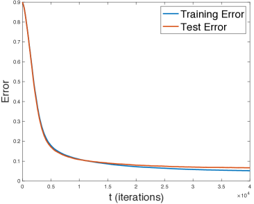
Figure 2: Example 2

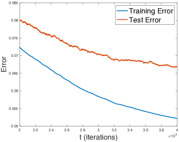
Figure 3: Example 2

Tuning the temperature parameter for simulating the Gibbs distribution is usually done with cross-validation [1, 13]. We leave for future work the problem of tuning the temperature vector for achieving low test error while having low mixing time. To simulate $P^{\star}_{W|S}$ for more than two layers, similar to line 6 of Algorithm 2, one can compute Monte Carlo approximations to the acceptance ratio of each layer, based on the samples from the next layers and the inner level algorithms. Various ideas could be used to decrease the running time of simulating the twisted distribution $P^{\star}_{W|S}$. In particular, one may use gradients as in Hamiltonian Monte Carlo [44, 45] and stochastic gradient Langevin dynamics [12], divide the training set into mini-batches with divide-and-conquer approaches, use sub-sampling methods [32], or simulate a variational Bayes approximation to the twisted distribution (see [46] for approximating the Gibbs distribution). We are currently invesitgating these directions.

Remark 3.

As a side result, in Appendix H, we show how to alternatively achieve the excess risk bound of Theorem 2 with an average predictor for the special case of binary classification with $\ell_{1}$ loss, based on an idea of [8].

8 Acknowledgement

We are grateful to Ramon van Handel for his generous time and for the many discussions on chaining.

Appendix A Information-theoretic tools

Definition 3 (Relative information).

Given probability measures $P$ and $Q$ defined on a measurable space $(\mathcal{A},\mathscr{F})$, such that $P\ll Q$, the relative information between $P$ and $Q$ in $a\in\mathcal{A}$ is the logarithm of the Radon–Nikodym derivative of $P$ with respect to $Q$:

$$\imath_{P\|Q}(a)=\log\frac{\mathrm{d}P}{\mathrm{d}Q}(a).$$

Definition 4 (Relative entropy).

The relative entropy between distributions $P$ and $Q$ defined on the same measurable space $(\mathcal{A},\mathscr{F})$, if $P\ll Q$ is

$$D(P\|Q)=\mathbb{E}[\imath_{P\|Q}(X)],\qquad X\sim P,$$

otherwise, we define $D(P\|Q)=\infty$.

Definition 5 (Conditional relative entropy).

The conditional relative entropy is defined as

$$D(P_{Y|X}\|Q_{Y|X}|P_{X}) =\int D(P_{Y|X=\omega}\|Q_{Y|X=\omega})\mathrm{d}P_{X}(\omega)$$

$$=\mathbb{E}[D(P_{Y|X}(\cdot|X)\|Q_{Y|X}(\cdot|X))],\quad X\sim P_{X}.$$

The following lemma is known as the chain rule of relative entropy. For a proof of this property of relative entropy, see e.g. [47, Theorem 2.5.3]:

Lemma 3 (Chain rule of relative entropy).

We have

$$D(P_{XY}\|Q_{XY})=D(P_{X}\|Q_{X})+D(P_{Y|X}\|Q_{Y|X}|P_{X}).$$

More generally,

$$D\left(P_{X_{1}\dots X_{n}}\|Q_{X_{1}\dots X_{n}}\right)=\sum_{i=1}^{n}D\left(P_{X_{i}|X_{1}\dots X_{i-1}}\|Q_{X_{i}|X_{1}\dots X_{i-1}}|P_{X_{1}\dots X_{i-1}}\right).$$

The following is a well-known property of mutual information:

Lemma 4 (Difference decomposition of mutual information).

For any $Q_{Y}$ such that $D(P_{Y}\|Q_{Y})<\infty$, we have

$$I(X;Y)=D(P_{Y|X}\|Q_{Y}|P_{X})-D(P_{Y}\|Q_{Y}).$$

We give the following general definition of Rényi divergence from [48]:

Definition 6 (Rényi divergence).

Given distributions $P$ and $Q$ defined on the same probability space, let probability measure $R$ be such that $P\ll R$ and $Q\ll R$, and let $Z\sim R$. Then, the Rényi divergence of order $\alpha\in(0,1)\cup(1,\infty)$ between $P$ and $Q$ is defined as

$$D_{\alpha}(P\|Q)=\frac{1}{\alpha-1}\log\mathbb{E}\left[\exp\left(\alpha\imath_{P\|R}(Z)+(1-\alpha)\imath_{Q\|R}(Z)\right)\right].$$

Due to its limiting behaviour, for $\alpha=1$ we define $D_{1}(P\|Q)=D(P\|Q)$.

For instance, for discrete distributions $P$ and $Q$ defined on a set $\mathcal{A}$ and for any $\alpha\in(0,1)\cup(1,\infty)$, we have

$$D_{\alpha}(P\|Q)=\frac{1}{\alpha-1}\log\left(\sum_{a\in\mathcal{A}}P^{\alpha}(a)Q^{1-\alpha}(a)\right).$$

Appendix B Chaining mutual information

In this section, we strengthen the results of [4]. First we give the necessary definitions:

Definition 7 (Subgaussian process).

The random process $\{X_{t}\}_{t\in T}$ on the metric space $(T,d)$ is called subgaussian if $\mathbb{E}[X_{t}]=0$ for all $t\in T$ and

$$\mathbb{E}[e^{\lambda(X_{t}-X_{s})}]\leq e^{\frac{1}{2}\lambda^{2}d^{2}(t,s)}\textrm{ \leavevmode\nobreak\ for all \leavevmode\nobreak\ }t,s\in T,\lambda\geq 0.$$

The following is a technical assumption which holds in almost all cases of interest:

Definition 8 (Separable process).

The random process $\{X_{t}\}_{t\in T}$ is called separable if there is a countable set $T_{0}\subseteq T$ such that $X_{t}\in\lim_{\begin{subarray}{c}s\rightarrow t\\ s\in T_{0}\end{subarray}}X_{s}$ for all $t\in T$ a.s., where $x\in\lim_{\begin{subarray}{c}s\rightarrow t\\ s\in T_{0}\end{subarray}}x_{s}$ means that there is a sequence $(s_{n})$ in $T_{0}$ such that $s_{n}\rightarrow t$ and $x_{s_{n}}\rightarrow x$.

For instance, if $t\to X_{t}$ is continuous almost surely, then $X_{t}$ is a separable process (see e.g. [33]).

Notice that, unlike a partition, an exact cover $\mathcal{P}=\{A_{i}:i\in M\}$ of the set $T$ may have countably or uncountably infinite number of blocks, i.e. $M$ may have countably or uncountably infinite size.

Definition 9 ($\epsilon$-cover).

We call a cover $\mathcal{P}=\{A_{i}:i\in M\}$ of the set $T$ an $\epsilon$-cover of the metric space $(T,d)$ if for all $i\in M$, $A_{i}$ can be contained withing a ball of radius $\epsilon$.

Definition 10 (Hierarchical sequence of covers).

A sequence of covers $\{\mathcal{P}_{k}\}_{k=m}^{\infty}$ of a set $T$ is called a hierarchical sequence (or an increasing sequence) if for all $k\geq m$ and each $A\in\mathcal{P}_{k+1}$, there exists $B\in\mathcal{P}_{k}$ such that $A\subseteq B$. For any such sequence of exact covers and any $t\in T$, let $[t]_{k}$ denote the unique set $A\in\mathcal{P}_{k}$ such that $t\in A$.

If $\mathcal{N}$ is a set, let $X_{\mathcal{N}}\triangleq\{X_{i}:i\in N\}$ denote a random process indexed by the elements of $\mathcal{N}$. For any bounded metric space $(S,d)$, let $k_{1}(S)$ be an integer such that $2^{-(k_{1}(S)-1)}\geq\mathrm{diam}(S)$.

Theorem 4.

Assume that $\{\mathrm{gen}(w)\}_{w\in\mathcal{W}}$ is a separable subgaussian process on the bounded metric space $(\mathcal{W},d)$. Let $\{\mathcal{P}_{k}\}_{k=k_{1}(\mathcal{W})}^{\infty}$ be a hierarchical sequence of exact coverings of $\mathcal{W}$, where for each $k\geq k_{1}(\mathcal{W})$, $\mathcal{P}_{k}$ is a $2^{-k}$-cover of $(\mathcal{W},d)$.

1. $$\mathrm{gen}(\mu,P_{W|S})\leq 3\sqrt{2}\sum_{k=k_{1}(\mathcal{W})}^{\infty}2^{-k}\sqrt{I([W]_{k};S)},$$

2. If $\mathbf{0}\in\{\ell(h_{w},\cdot):w\in\mathcal{W}\}$, then

   $$\mathrm{gen^{+}}(\mu,P_{W|S})\leq 3\sqrt{2}\sum_{k=k_{1}(\mathcal{W})}^{\infty}2^{-k}\sqrt{I([W]_{k};S)+\log 2},$$

   where $\mathbf{0}$ is a function identically equal to zero and $\mathrm{gen}^{+}(\mu,P_{W|S})\triangleq\mathbb{E}\left[|L_{\mu}(W)-L_{S}(W)|\right]$.

Theorem 4 is in the context of statistical learning. The more general counterpart in the context of random processes is Theorem 5:

Theorem 5.

Assume that $\{X_{t}\}_{t\in T}$ is a separable subgaussian process on the bounded metric space $(T,d)$. Let $\{\mathcal{P}_{k}\}_{k=k_{1}(T)}^{\infty}$ be a hierarchical sequence of exact coverings of $T$, where for each $k\geq k_{1}(T)$, $\mathcal{P}_{k}$ is a $2^{-k}$-cover of $(T,d)$. Let $W$ be a random variable taking values from $T$.

1. $$\mathbb{E}[X_{W}]\leq 3\sqrt{2}\sum_{k=k_{1}(T)}^{\infty}2^{-k}\sqrt{I([W]_{k};X_{T})}.$$

2. For any arbitrary $t_{0}\in T$,

   $$\mathbb{E}[|X_{W}-X_{t_{0}}|]\leq 3\sqrt{2}\sum_{k=k_{1}(T)}^{\infty}2^{-k}\sqrt{I([W]_{k};X_{T})+\log 2}.$$

Proof of Theorem 5.

For an arbitrary $k\geq k_{1}(T)$, consider $\mathcal{P}_{k}=\{A^{(k)}_{i}:i\in M_{k}\}$. Since $\mathcal{P}_{k}$ is a $2^{-k}$-cover of $(T,d)$, based on Definition 9, there exists a multi-set $\mathcal{N}_{k}\triangleq\{a_{i}:i\in M_{k}\}\subseteq T$ and a mapping $\pi_{\mathcal{N}_{k}}:T\to\mathcal{N}_{k}$ such that $\pi_{\mathcal{N}_{k}}(t)=a_{i}$ if $t\in A_{i}^{(k)}$ for all $i\in M_{k}$, and $d\left(t,\pi_{\mathcal{N}_{k}}(t)\right)\leq 2^{-k}$ for all $t\in T$. For an arbitrary $t_{0}\in T$, let $\mathcal{N}_{k_{0}}\triangleq\{t_{0}\}$. For any integer $n\geq k_{1}(T)$, we can write

$$X_{W}=X_{t_{0}}+\sum_{k=k_{1}(T)}^{n}\left(X_{\pi_{\mathcal{N}_{k}}(W)}-X_{\pi_{\mathcal{N}_{k-1}}(W)}\right)+\left(X_{W}-X_{\pi_{\mathcal{N}_{n}}(W)}\right).$$

Based on the definition of subgaussian processes, the process is centered, thus $\mathbb{E}[X_{t_{0}}]=0$. Therefore

$$\mathbb{E}[X_{W}]-\mathbb{E}\left[X_{W}-X_{\pi_{\mathcal{N}_{n}}(W)}\right]=\sum_{k=k_{1}(T)}^{n}\mathbb{E}\left[X_{\pi_{\mathcal{N}_{k}}(W)}-X_{\pi_{\mathcal{N}_{k-1}}(W)}\right].$$

For every $k\geq k_{1}(T)$ and $t\in T$, based on the triangle inequality,

$$d\left(\pi_{\mathcal{N}_{k}}(t),\pi_{\mathcal{N}_{k-1}}(t)\right) \leq d\left(t,\pi_{\mathcal{N}_{k}}(t)\right)+d\left(t,\pi_{\mathcal{N}_{k-1}}(t)\right)$$

$$\leq 3\times 2^{-k}.$$

Knowing the value of $\left(\pi_{\mathcal{N}_{k}}(W),\pi_{\mathcal{N}_{k-1}}(W)\right)$ is sufficient to determine which one of the random variables $\left\{X_{\pi_{\mathcal{N}_{k}}(t)}-X_{\pi_{\mathcal{N}_{k-1}}(t)}\right\}_{t\in T}$ is chosen according to $W$. Therefore
$\left(\pi_{\mathcal{N}_{k}}(W),\pi_{\mathcal{N}_{k-1}}(W)\right)$ is playing the role of the random index, and since $X_{\pi_{\mathcal{N}_{k}}(t)}-X_{\pi_{\mathcal{N}_{k-1}}(t)}$ is $d^{2}\left(\pi_{\mathcal{N}_{k}}(t),\pi_{\mathcal{N}_{k-1}}(t)\right)$-subgaussian, based on Theorem 2 of [3], an application of the data processing inequality and by summation, we have

$$\sum_{k=k_{1}(T)}^{n}\mathbb{E}\left[X_{\pi_{\mathcal{N}_{k}}(W)}-X_{\pi_{\mathcal{N}_{k-1}}(W)}\right]\leq\sum_{k=k_{1}(T)}^{n}3\sqrt{2}\times 2^{-k}\sqrt{I(\pi_{\mathcal{N}_{k}}(W),\pi_{\mathcal{N}_{k-1}}(W);X_{T})}.$$

Since $\{\mathcal{P}_{k}\}_{k=k_{1}(T)}^{\infty}$ is a hierarchical sequence of coverings, for any $t\in T$, knowing $\mathcal{N}_{k}(t)$ will uniquely determine $\mathcal{N}_{k-1}(t)$. Therefore

$$I\left(\pi_{\mathcal{N}_{k}}(W),\pi_{\mathcal{N}_{k-1}}(W);X_{T}\right) =I\left(\pi_{\mathcal{N}_{k}}(W);X_{T}\right)$$

$$=I\left([W]_{k};X_{T}\right).$$

The rest of the proof follows from the definition of separable processes and the fact that

$$\lim_{n\to\infty}\mathbb{E}\left[X_{W}-X_{\pi_{\mathcal{N}_{n}}(W)}\right]=0.$$

∎

If in Theorem 5, we let $T\triangleq\mathcal{W}$ and $X_{w}\triangleq\mathrm{gen}(w)$ for all $w\in\mathcal{W}$, then for each $k\geq k_{1}(T)$, due to the Markov chain

$$X_{T}=\{\mathrm{gen}(w)\}_{w\in\mathcal{W}}\leftrightarrow S\leftrightarrow W\leftrightarrow[W]_{k}$$ (12)

and the data processing inequality, we deduce $I([W]_{k};X_{T})\leq I([W]_{k};S)$. Therefore Theorem 4 follows from Theorem 5.

If we use Theorem 2 of [19] instead of Theorem 2 of [3], then we can tighten the bound of Theorem 4 to the following result. Recall that $S=(Z_{1},\dots,Z_{n})$ denotes the training set.

Proposition 1.

Assume that $\{\mathrm{gen}(w)\}_{w\in\mathcal{W}}$ is a separable subgaussian process on the bounded metric space $(\mathcal{W},d)$. Let $\{\mathcal{P}_{k}\}_{k=k_{1}(\mathcal{W})}^{\infty}$ be an increasing sequence of partitions of $\mathcal{W}$, where for each $k\geq k_{1}(\mathcal{W})$, $\mathcal{P}_{k}$ is a $2^{-k}$-partition of $(\mathcal{W},d)$. Then

$$\mathrm{gen}(\mu,P_{W|S})\leq 3\sqrt{2}\sum_{k=k_{1}(\mathcal{W})}^{\infty}2^{-k}\left(\sum_{i=1}^{n}\sqrt{I([W]_{k};Z_{i})}\right),$$ (13)

Appendix C Proofs of generalization and excess risk bounds

Proof of Lemma 1.

Since $\phi$ is $1$-Lipschitz and $\phi(0)=0$, for all vectors $x$ we have $|\phi(x)|_{2}\leq|x|_{2}$. Based on the triangle inequality, for all $1\leq i\leq k-1$, we can write

$$\|\mathbf{W}_{i}\|_{2} \leq\|\mathbf{W}_{i}-M_{i}\|_{2}+\|M_{i}\|_{2}$$

$$\leq(\alpha_{i}+1)\|M_{i}\|_{2}$$

$$\leq\exp(\alpha_{i})\|M_{i}\|_{2}.$$

Thus, for all $x^{m}\in\mathcal{X}$,

$$|\sigma(\mathbf{W}_{k-1}(\dots\sigma(\mathbf{W}_{1}(x^{m}))\dots))|_{2}\leq\exp\left(\sum_{i=1}^{k-1}\alpha_{i}\right)\left(\prod_{i=1}^{k-1}\|M_{i}\|_{2}\right)|x^{m}|_{2}.$$

This yields

$$|\sigma(\mathbf{W}_{k}(\dots(\sigma(\mathbf{W}_{1}(x^{m}))\dots)))- \sigma(M_{k}(\dots(\sigma(\mathbf{W}_{1}(x^{m}))\dots)))|_{2}$$

$$\leq\exp\left(\sum_{i=1}^{k-1}\alpha_{i}\right)\left(\prod_{i=1}^{k-1}\|M_{i}\|_{2}\right)\|\mathbf{W}_{k}-M_{k}\|_{2}|x^{m}|_{2}$$

$$\leq\alpha_{k}\exp\left(\sum_{i=1}^{k-1}\alpha_{i}\right)\left(\prod_{i=1}^{k}\|M_{i}\|_{2}\right)|x^{m}|_{2}.$$

Since $M_{i}$ is $\|M_{i}\|_{2}$-Lipschitz for all $k+1\leq i\leq d$, and soft-max is $1$-Lipschitz with respect to the Euclidean norm (see e.g. [49]), we conclude that

$$|h_{w_{1}}(x^{m})-h_{w_{2}}(x^{m})|_{2}\leq\alpha_{k}\exp\left(\sum_{i=1}^{k-1}\alpha_{i}\right)M|x^{m}|_{2}.$$

∎

Definition 11.

For all $1\leq k\leq d$, let

$$h_{[\mathbf{W}_{1},\dots,\mathbf{W}_{k}]}\triangleq h_{[\mathbf{W}_{1},\dots,\mathbf{W}_{k},M_{k+1},\dots,M_{d}]}$$

and

$$\ell([\mathbf{W}_{1},\dots,\mathbf{W}_{k}],z)\triangleq\ell([\mathbf{W}_{1},\dots,\mathbf{W}_{k},M_{k+1},\dots,M_{d}],z).$$

Proof of Theorem 1.

Based on the Azuma–Hoeffding inequality, $\{\mathrm{gen}(w)\}_{w\in\mathcal{W}}$ is a subgaussian process with the metric

$$d(w,w^{\prime})\triangleq\frac{\|\ell({w},\cdot)-\ell({w^{\prime}},\cdot)\|_{\infty}}{\sqrt{n}},$$

regardless of the choice of distribution $\mu$ on $\mathsf{Z}$. For any example $z=(x^{m},y)\in\mathsf{Z}$, we have

$$|\ell(w,z)-\ell(w^{\prime},z)|\leq L\left|h_{w}(x^{m})-h_{w^{\prime}}(x^{m})\right|_{2}.$$

Therefore

$$\|\ell(w,\cdot)-\ell(w^{\prime},\cdot)\|_{\infty}\leq L\sup_{x^{m}\in\mathcal{X}}|h_{w}(x^{m})-h_{w^{\prime}}(x^{m})|_{2}.$$ (14)

To apply the CMI technique, we write the following chaining sum:

$$\mathrm{gen}(W) =\mathrm{gen}(W_{1})+(\mathrm{gen}(W_{1},W_{2})-\mathrm{gen}(W_{1}))+\dots$$

$$\quad+(\mathrm{gen}(W)-\mathrm{gen}(W_{1},\dots,W_{d-1})).$$

Taking expectations with respect to $P_{WS}$ yields

$$\mathrm{gen}(\mu,P_{W|S})=\mathbb{E}[\mathrm{gen}(W)] =\mathbb{E}[\mathrm{gen}(W_{1})]+\mathbb{E}[\mathrm{gen}(W_{1},W_{2})-\mathrm{gen}(W_{1})]+\dots$$

$$\quad+\mathbb{E}[\mathrm{gen}(W)-\mathrm{gen}(W_{1},\dots,W_{d-1})],$$ (15)

Based on Lemma 1, for all $1\leq k\leq d$, we have

$$\sup_{x^{m}\in\mathcal{X}}|h_{[\mathbf{W}_{1},\dots,\mathbf{W}_{k}]}(x^{m})-h_{[\mathbf{W}_{1},\dots,\mathbf{W}_{k-1}]}(x^{m})|_{2}\leq\beta_{k}MR.$$ (16)

Using (14), we deduce

$$\|\ell([\mathbf{W}_{1},\dots,\mathbf{W}_{k}],\cdot)-\ell([\mathbf{W}_{1},\dots,\mathbf{W}_{k-1}],\cdot)\|_{\infty}\leq L\beta_{k}MR.$$ (17)

Notice that knowing the value of $(W_{1},\dots,W_{k})$ is enough to determine which one of the random variables $\left\{\mathrm{gen}(\mathbf{W}_{1},\dots,\mathbf{W}_{k})-\mathrm{gen}(\mathbf{W}_{1},\dots,\mathbf{W}_{k-1})\right\}_{w\in\mathcal{W}}$ is chosen according to $W$. Therefore $(W_{1},\dots,W_{k})$ is playing the role of the random index, and since

$$\mathrm{gen}(\mathbf{W}_{1},\dots,\mathbf{W}_{k})-\mathrm{gen}(\mathbf{W}_{1},\dots,\mathbf{W}_{k-1})$$

is $d^{2}\left([\mathbf{W}_{1},\dots,\mathbf{W}_{k}],[\mathbf{W}_{1},\dots,\mathbf{W}_{k-1}]\right)$-subgaussian, based on (17), Theorem 2 of [3] and an application of the data processing inequality on the Markov chain $\{\mathrm{gen}(w)\}_{w\in\mathcal{W}}\leftrightarrow S\leftrightarrow W\leftrightarrow(W_{1},\dots,W_{k})$, we obtain

$$\mathbb{E}[\mathrm{gen}(W_{1},\dots,W_{k})-\mathrm{gen}(W_{1},\dots,W_{k-1})]\leq\frac{LMR\sqrt{2}\beta_{k}}{\sqrt{n}}\sqrt{I(S;W_{1},\dots,W_{k})}.$$ (18)

From (15) and (18) we deduce

$$\mathrm{gen}(\mu,P_{W|S})=\mathbb{E}[\mathrm{gen}(W)]\leq\frac{LMR\sqrt{2}}{\sqrt{n}}\sum_{k=1}^{d}\beta_{k}\sqrt{I(S;W_{1},\dots,W_{k})}.$$

∎

Proof of Theorem 2.

By plugging in $P_{W_{1}\dots W_{k}|S}\leftarrow\delta_{\widehat{w}_{1}\dots\widehat{w}_{k}}$ in the right side of (6), and by noting that $P_{W|S}^{\star}$ is defined as the conditional distribution which minimizes that expression, we obtain (8). ∎

In the following, the notation $P_{X}\to Q_{Y|X}\to P_{Y}$ indicates that the joint distribution of $X$ and $Y$ is $P_{XY}=P_{X}Q_{Y|X}$. We state a high-probability result:

Corollary 1.

For a given $\mu$, let $\widehat{w}(\mu)$ denote the index of a hypothesis which achieves the minimum statistical risk among $\mathcal{W}$. If $P_{S}\to P_{W|S}^{\star}\to P_{W}$, then

$$\mathbb{P}\left[L_{\mu}(W)\leq\inf_{w\in\mathcal{W}}L_{\mu}(w)+\epsilon\right]\geq 1-\frac{C}{\epsilon\sqrt{n}}\sum_{k=1}^{d}\beta_{k}\left(\gamma_{k}D\left(\delta_{\widehat{w}_{1}\dots\widehat{w}_{k}}\middle\|Q^{(k)}_{W_{1}\dots W_{k}}\right)+\frac{1}{4\gamma_{k}}\right).$$ (19)

Proof.

Based on Theorem 2, we have

$$\mathbb{E}[L_{\mu}(W)]-\inf_{w\in\mathcal{W}}L_{\mu}(w)\leq\frac{C}{\sqrt{n}}\sum_{k=1}^{d}\beta_{k}\left(\gamma_{k}D\left(\delta_{\widehat{w}_{1}\dots\widehat{w}_{k}}\middle\|Q^{(k)}_{W_{1}\dots W_{k}}\right)+\frac{1}{4\gamma_{k}}\right).$$

Thus

$$\mathbb{E}\left[L_{\mu}(W)-\inf_{w\in\mathcal{W}}L_{\mu}(w)\right]\leq\frac{C}{\sqrt{n}}\sum_{k=1}^{d}\beta_{k}\left(\gamma_{k}D\left(\delta_{\widehat{w}_{1}\dots\widehat{w}_{k}}\middle\|Q^{(k)}_{W_{1}\dots W_{k}}\right)+\frac{1}{4\gamma_{k}}\right).$$

Since $L_{\mu}(W)-\inf_{w\in\mathcal{W}}L_{\mu}(w)$ is a positive random variable, by Markov’s inequality we obtain

$$\mathbb{P}\left[L_{\mu}(W)-\inf_{w\in\mathcal{W}}L_{\mu}(w)>\epsilon\right]\leq\frac{C}{\epsilon\sqrt{n}}\sum_{k=1}^{d}\beta_{k}\left(\gamma_{k}D\left(\delta_{\widehat{w}_{1}\dots\widehat{w}_{k}}\middle\|Q^{(k)}_{W_{1}\dots W_{k}}\right)+\frac{1}{4\gamma_{k}}\right),$$

which yields

$$\mathbb{P}\left[L_{\mu}(W)\leq\inf_{w\in\mathcal{W}}L_{\mu}(w)+\epsilon\right]\geq 1-\frac{C}{\epsilon\sqrt{n}}\sum_{k=1}^{d}\beta_{k}\left(\gamma_{k}D\left(\delta_{\widehat{w}_{1}\dots\widehat{w}_{k}}\middle\|Q^{(k)}_{W_{1}\dots W_{k}}\right)+\frac{1}{4\gamma_{k}}\right).$$

∎

For the case of $\mathcal{W}$ being an arbitrary set, we state the following excess risk bound, whose proof is analogous to the proof of Theorem 2:

Proposition 2.

Assume that $\mathcal{W}$ is an arbitrary set and for a given input distribution $\mu$, let $\widehat{w}(\mu)$ denote the index of a hypothesis which achieves the minimum statistical risk among $\mathcal{W}$. Let $B^{(\epsilon)}_{W_{1}\dots W_{d}}$ denote the uniform distribution over a neighborhood $U_{\epsilon}$ of $\widehat{w}(\mu)$ for which all $w\in U_{\epsilon}$ satisfy $L_{\mu}(w)\leq\inf_{w\in\mathcal{W}}L_{\mu}(w)+\epsilon$. Then

$$\mathrm{risk}\left(\mu,P_{W|S}^{\star}\right)\leq\inf_{w\in\mathcal{W}}L_{\mu}(w)+\epsilon+\frac{C}{\sqrt{n}}\sum_{k=1}^{d}\beta_{k}\left(\gamma_{k}D\left(B^{(\epsilon)}_{W_{1}\dots W_{k}}\middle\|Q^{(k)}_{W_{1}\dots W_{k}}\right)+\frac{1}{4\gamma_{k}}\right).$$ (20)

Proof.

By plugging in $P_{W_{1}\dots W_{k}|S}\leftarrow B^{(\epsilon)}_{W_{1}\dots W_{k}}$ in the right side of (6), and by noting that $P_{W|S}^{\star}$ is defined as the conditional distribution which minimizes that expression, we obtain (20). ∎

Appendix D Gibbs distribution results

Definition 12 (Gibbs distribution).

The Gibbs (posterior) distribution associated to parameter $\gamma$ and prior distribution $Q$, is denoted with $P^{\gamma,Q}_{W|S}$ and defined as follows:

$$P^{\gamma,Q}_{W|S=s}(\mathrm{d}w)\triangleq\frac{e^{-\gamma L_{s}(w)}Q(\mathrm{d}w)}{\mathbb{E}[e^{-\gamma L_{s}(\widetilde{W})}]},\qquad\widetilde{W}\sim Q.$$

Lemma 5.

[3] The Gibbs distribution $P^{\gamma,Q}_{W|S}$ is the unique solution to the optimization problem

$$\operatorname*{arg\,min}_{P_{W|S}}\left\{\mathbb{E}[L_{S}(W)]+\frac{1}{\gamma}D(P_{W|S}\|Q|P_{S})\right\}.$$

The next results are new excess risk bounds for the Gibbs distribution:

Proposition 3.

Assume that $\mathcal{W}$ is a countable set. For any input distribution $\mu$, let $\widehat{w}(\mu)$ denote the index of a hypothesis which achieves the minimum statistical risk among $\mathcal{W}$. If for all $w\in\mathcal{W}$, $\ell(w,Z)$ is $\sigma^{2}$-subgaussian where $Z\sim\mu$, then for any $\gamma>0$,

$$\mathrm{risk}\left(\mu,P_{W|S}^{\gamma,Q}\right)\leq\inf_{w\in\mathcal{W}}L_{\mu}(w)+\frac{1}{\gamma}D\left(\delta_{\widehat{w}(\mu)}\middle\|Q\right)+\frac{\gamma\sigma^{2}}{2n}.$$ (21)

Proof.

Assuming $\mu^{\otimes n}=P_{S}\to P_{W|S}^{\gamma,Q}\to P_{W}$, we can write

$$\mathrm{risk}\left(\mu,P_{W|S}^{\gamma,Q}\right) =\mathbb{E}[L_{\mu}(W)]$$

$$\leq\mathbb{E}[L_{S}(W)]+\sqrt{\frac{2\sigma^{2}}{n}}.\sqrt{I(S;W)}$$

$$\leq\mathbb{E}[L_{S}(W)]+\sqrt{\frac{2\sigma^{2}}{n}}\left(\frac{1}{\gamma}\sqrt{\frac{n}{2\sigma^{2}}}I(S;W)+\frac{1}{4\frac{1}{\gamma}\sqrt{\frac{n}{2\sigma^{2}}}}\right)$$ (22)

$$=\mathbb{E}[L_{S}(W)]+\frac{1}{\gamma}I(S;W)+\frac{\gamma\sigma^{2}}{2n}$$

$$\leq\mathbb{E}[L_{S}(W)]+\frac{1}{\gamma}D\left(P_{W|S}^{\gamma,Q}\middle\|Q\middle|P_{S}\right)+\frac{\gamma\sigma^{2}}{2n}$$

$$\leq\inf_{w\in\mathcal{W}}L_{\mu}(w)+\frac{1}{\gamma}D\left(\delta_{\widehat{w}(\mu)}\middle\|Q\right)+\frac{\gamma\sigma^{2}}{2n},$$ (23)

where (22) follows from the inequality

$$\sqrt{x}\leq cx+\frac{1}{4c}\iff 0\leq\left(\sqrt{cx}-\frac{1}{2\sqrt{c}}\right)^{2}\qquad\mathrm{for\ all\ }x,c>0,$$ (24)

which is upper bounding $\sqrt{x}$ with a tangent line, and (23) follows from Lemma 5 and by plugging $P_{W|S}\leftarrow\delta_{\widehat{w}(\mu)}$ into

$$\mathbb{E}[L_{S}(W)]+\frac{1}{\gamma}D(P_{W|S}\|Q|P_{S}).$$

∎

Corollary 2.

If we set $\gamma\leftarrow\frac{1}{\sigma}\sqrt{2nD\left(\delta_{\widehat{w}(\mu)}\middle\|Q\right)}\triangleq\gamma^{\star}$, then we minimize the right side of (21) to obtain

$$\mathrm{risk}\left(\mu,P_{W|S}^{Q,\gamma^{\star}}\right)\leq\inf_{w\in\mathcal{W}}L_{\mu}(w)+\sigma\sqrt{\frac{D\left(\delta_{\widehat{w}(\mu)}\middle\|Q\right)}{2n}}.$$

Proposition 4.

Assume that $\mathcal{W}$ is an uncountable set. For any input distribution $\mu$, let $\widehat{w}(\mu)$ denote the index of a hypothesis which achieves the minimum statistical risk among $\mathcal{W}$. If for all $w\in\mathcal{W}$, $\ell(w,Z)$ is $\sigma^{2}$-subgaussian where $Z\sim\mu$ and $\ell(\cdot,z)$ is $\rho$-Lipschitz for all $z\in\mathsf{Z}$, then for any $\gamma>0$,

$$\mathrm{risk}\left(\mu,P_{W|S}^{\gamma,Q}\right)\leq\inf_{w\in\mathcal{W}}L_{\mu}(w)+\inf_{a>0}\left(a\rho\sqrt{d}+\frac{1}{\gamma}D\left(\mathcal{N}\left(\widehat{w}(\mu),a^{2}I_{d}\right)\middle\|Q\right)\right)+\frac{\gamma\sigma^{2}}{2n},$$

where $\mathcal{N}\left(\widehat{w}(\mu),a^{2}I_{d}\right)$ denotes the Gaussian distribution centered at $\widehat{w}(\mu)$ with covariance matrix $a^{2}I_{d}$.

Proof.

Assuming $\mu^{\otimes n}=P_{S}\to P_{W|S}^{\gamma,Q}\to P_{W}$, we can write

$$\mathrm{risk}\left(\mu,P_{W|S}^{\gamma,Q}\right) =\mathbb{E}[L_{\mu}(W)]$$

$$\leq\mathbb{E}[L_{S}(W)]+\sqrt{\frac{2\sigma^{2}}{n}}.\sqrt{I(S;W)}$$

$$\leq\mathbb{E}[L_{S}(W)]+\sqrt{\frac{2\sigma^{2}}{n}}\left(\frac{1}{\gamma}\sqrt{\frac{n}{2\sigma^{2}}}I(S;W)+\frac{1}{4\frac{1}{\gamma}\sqrt{\frac{n}{2\sigma^{2}}}}\right)$$ (25)

$$=\mathbb{E}[L_{S}(W)]+\frac{1}{\gamma}I(S;W)+\frac{\gamma\sigma^{2}}{2n}$$

$$\leq\mathbb{E}[L_{S}(W)]+\frac{1}{\gamma}D\left(P_{W|S}^{\gamma,Q}\middle\|Q\middle|P_{S}\right)+\frac{\gamma\sigma^{2}}{2n}$$

$$\leq\inf_{w\in\mathcal{W}}L_{\mu}(w)+\inf_{a>0}\left(a\rho\sqrt{d}+\frac{1}{\gamma}D\left(\mathcal{N}(\widehat{w}(\mu),a^{2}I_{d})\|Q\right)\right)+\frac{\gamma\sigma^{2}}{2n},$$ (26)

where (25) follows from the inequality (24), and (26) follows from Lemma 5 and by plugging $P_{W|S}\leftarrow\mathcal{N}\left(\widehat{w}(\mu),a^{2}I_{d}\right)$ into

$$\mathbb{E}[L_{S}(W)]+\frac{1}{\gamma}D(P_{W|S}\|Q|P_{S}),$$

while writing

$$\mathbb{E}[L_{S}(W)] \leq\inf_{w\in\mathcal{W}}L_{\mu}(w)+a\rho\sqrt{d}$$ (27)

and taking infimum over $a>0$. Inequality (27) is based on the proof of [3, Corollary 3]. ∎

More generally, in the context of empirical processes, let $\mathcal{F}=\{f_{w}:w\in\mathcal{W}\}$ be a collection of measurable functions from a set $\mathsf{Z}$ to $\mathbb{R}$, indexed by the set $\mathcal{W}$. Let $Z_{1},Z_{2},\dots,Z_{n}$ be a sequence of i.i.d elements drawn from $\mathsf{Z}$ with distribution $\mu$, and define $S=(Z_{1},\dots,Z_{n})$. For each $w\in\mathcal{W}$, define the empirical mean of function $f_{w}$ as

$$\mu_{n}(f_{w})\triangleq\frac{1}{n}\sum_{i=1}^{n}f_{w}(Z_{i}),$$

and its true mean as

$$\mu(f_{w})\triangleq\mathbb{E}\left[f_{w}(Z)\right],\quad Z\sim\mu.$$

One can prove the following proposition, analogous to the poof of Proposition 3:

Proposition 5.

Assume that $\mathcal{W}$ is a countable set. For any input distribution $\mu$, let $\widehat{w}(\mu)$ denote the index of a function which has the minimum true mean among functions in $\mathcal{F}$. If $f_{w}(Z),\ Z\sim\mu$ is $\sigma^{2}$-subgaussian for all $w\in\mathcal{W}$, then for any $\gamma>0$,

$$\mathbb{E}\left[\mu(f_{W})\right]\leq\inf_{w\in\mathcal{W}}\mu(f_{w})+\frac{1}{\gamma}D(\delta_{\widehat{w}(\mu)}\|Q)+\frac{\gamma\sigma^{2}}{2n},$$

where $\mu^{\otimes n}=P_{S}\to P^{\gamma,Q}_{W|S}\to P_{W}$.

Appendix E Proof for the MT algorithm

We first state the following lemmas. Lemma 6 shows the useful role of tilted distributions in linearly combining relative entropies. For a proof, see [43, Theorem 30].

Lemma 6.

Let $\lambda\in[0,1]$. For any $P\ll Q$ and $P\ll R$,

$$\lambda D(P\|Q)+(1-\lambda)D(P\|R)=D\left(P\|(Q,R)_{\lambda}\right)+(1-\lambda)D_{\lambda}(Q\|R),$$

where $(Q,R)_{\lambda}$ denotes the tilted distribution. Therefore

$$\operatorname*{arg\,min}_{P}\left\{\lambda D(P\|Q)+(1-\lambda)D(P\|R)\right\}=(Q,R)_{\lambda},$$

and

$$\min_{P}\left\{\lambda D(P\|Q)+(1-\lambda)D(P\|R)\right\}=(1-\lambda)D_{\lambda}(Q\|R).$$

The next lemma is a crucial property of conditional relative entropy:

Lemma 7.

Given distribution $P_{X}$ defined on a set $\mathcal{A}$ and conditional distributions $P_{Y|X}$ and $Q_{Y|X}$, we have

$$D(P_{Y|X}\|Q_{Y|X}|P_{X})\geq 0,$$ (28)

with equality if and only if $P_{Y|X}=Q_{Y|X}$ holds on a set $\mathcal{A}^{\prime}\subseteq\mathcal{A}$ of conditioning values with $P_{X}(\mathcal{A}^{\prime})=1$.

The simplest case of (10) is when $d=2$, whose solution, characterized by the following result, is useful for obtaining the solution to the general case:

Proposition 6.

Let $Q_{X}$ and $R_{XY}$ be two arbitrary distributions. For any $a_{1},a_{2}>0$, we have

$$\operatorname*{arg\,min}_{P_{XY}}\left(a_{1}D(P_{X}\|Q_{X})+a_{2}D(P_{XY}\|R_{XY})\right)=P^{\star}_{XY},$$ (29)

where

$$\begin{cases}P^{\star}_{X}=(Q_{X},R_{X})_{\frac{a_{1}}{a_{1}+a_{2}}},\\ P^{\star}_{Y|X}=R_{Y|X}.\end{cases}$$

Proof.

Based on the chain rule of relative entropy, we have

$$D(P_{XY}\|R_{XY})=D(P_{X}\|R_{X})+D(P_{Y|X}\|R_{Y|X}|P_{X}).$$

Therefore

$$a_{1}D(P_{X}\|Q_{X})+a_{2}D(P_{XY}\|R_{XY})$$

$$=a_{1}D(P_{X}\|Q_{X})+a_{2}(D(P_{X}\|R_{X})+D(P_{Y|X}\|R_{Y|X}|P_{X}))$$

$$=(a_{1}D(P_{X}\|Q_{X})+a_{2}D(P_{X}\|R_{X}))+a_{2}D(P_{Y|X}\|R_{Y|X}|P_{X})$$

$$=(a_{1}+a_{2})D\left(P_{X}\middle\|(Q_{X},R_{X})_{\frac{a_{1}}{a_{1}+a_{2}}}\right)+a_{2}D_{\frac{a_{1}}{a_{1}+a_{2}}}(Q_{X}\|R_{X})+a_{2}D(P_{Y|X}\|R_{Y|X}|P_{X}),$$ (30)

where (30) is based on Lemma 6. Note that, due to Lemma 7, distribution $P^{\star}_{XY}$ is the unique distribution for which both relative entropies vanish simultaneously, and since the Rényi divergence does not depend on $P_{XY}$, equation (29) is proven. ∎

Inspired by the proof of Proposition 6, we now give the proof of the general case:

Proof of Theorem 3.

Similar to Proposition 6, for the general case of arbitrary $d\geq 3$, we can solve (10) backwards and iteratively:

$$\sum_{i=1}^{d}a_{i}D\left(P_{X_{1}\dots X_{i}}\|R^{(i)}_{X_{1}\dots X_{i}}\right)$$

$$=\sum_{i=1}^{d-1}a_{i}D\left(P_{X_{1}\dots X_{i}}\middle\|R^{(i)}_{X_{1}\dots X_{i}}\right)$$

$$\qquad+a_{d}\left(D\left(P_{X_{1}\dots X_{d-1}}\middle\|R^{(d)}_{X_{1}\dots X_{d-1}}\right)+D\left(P_{X_{d}|X_{1}\dots X_{d-1}}\middle\|R^{(d)}_{X_{d}|X_{1}\dots X_{d-1}}\middle|P_{X_{1}\dots X_{d-1}}\right)\right)$$

$$=\sum_{i=1}^{d-2}a_{i}D\left(P_{X_{1}\dots X_{i}}\middle\|R^{(i)}_{X_{1}\dots X_{i}}\right)$$

$$\quad+(a_{d-1}+a_{d})D\left(P_{X_{1}\dots X_{d-1}}\middle\|\left(R_{X_{1}\dots X_{d-1}}^{(d-1)},R_{X_{1}\dots X_{d-1}}^{(d)}\right)_{\frac{a_{d-1}}{a_{d-1}+a_{d}}}\right)$$

$$\quad+a_{d}D_{\frac{a_{d-1}}{a_{d-1}+a_{d}}}\left(R_{X_{1}\dots X_{d-1}}^{(d-1)}\middle\|R_{X_{1}\dots X_{d-1}}^{(d)}\right)$$

$$\quad+a_{d}D\left(P_{X_{d}|X_{1}\dots X_{d-1}}\middle\|R^{(d)}_{X_{d}|X_{1}\dots X_{d-1}}\middle|P_{X_{1}\dots X_{d-1}}\right),$$ (31)

where (31) follows from Lemma 6. Notice that we can set

$$P^{\star}_{X_{d}|X_{1}\dots X_{d-1}}\leftarrow R^{(d)}_{X_{d}|X_{1}\dots X_{d-1}}=S^{(d)}_{X_{d}|X_{1}\dots X_{d-1}},$$

to make the last conditional relative entropy in the right side of (31) vanish (and hence minimized, due to Lemma 7), regardless of any choice for $P_{X_{1}\dots X_{d-1}}$ that we may take later on. Since the Rényi divergence in (31) does not depend on $P_{X_{1}\dots X_{d}}$, we can ignore that term, and repeat this process to the sum of the remaining terms iteratively to obtain $P^{\star}_{X_{i}|X_{1}\dots X_{i-1}}=S^{(i)}_{X_{i}|X_{1}\dots X_{i-1}}$ for all $1\leq i\leq d-1$, where intermediate distributions $S^{(i)}_{X_{1}\dots X_{i}}$ are defined as in Algorithm 1. In view of the fact that

$$P^{\star}_{X_{1}\dots X_{d}}=P^{\star}_{X_{1}}P^{\star}_{X_{2}|X_{1}}\dots P^{\star}_{X_{d}|X_{1}\dots X_{d-1}},$$

we have obtained the desired distribution $P^{\star}_{X_{1}\dots X_{d}}$ as

$$P^{\star}_{X_{1}\dots X_{d}}=S^{(1)}_{X_{1}}S^{(2)}_{X_{2}|X_{1}}\dots S^{(d)}_{X_{d}|X_{1}\dots X_{d-1}}.$$

∎

The key point of the previous proof is to rewrite the expression in (10) as the sum of some Rényi divergences which do not depend on $P_{X_{1}\dots X_{d}}$, and some conditional relative entropies which can all be set equal to zero, simultaneously. Based on Lemma 7, this happens if and only if $P_{X_{1}\dots X_{d}}=P^{\star}_{X_{1}\dots X_{d}}$, up to almost sure equality.

Appendix F The multilevel Metropolis algorithm

Using the MT algorithm, we derive the twisted distribution $P^{\star}_{W|S}$ for a two-layer net with prior distribution $Q^{(1)}_{W_{1}}$ and $Q^{(2)}_{W_{1}W_{2}}$, and temperature vector $(a_{1},a_{2})$, as

$$P^{\star}_{W|S=s}(w_{1},w_{2}) =\frac{\left(\bigintsss_{v_{2}}f(w_{1},v_{2})^{\frac{1}{a_{2}}}Q^{(2)}(w_{1},v_{2})\mathrm{d}v_{2}\right)^{\frac{a_{2}}{a_{1}+a_{2}}}Q^{(1)}(w_{1})^{\frac{a_{1}}{a_{1}+a_{2}}}}{\bigintsss_{v_{1}}\left(\bigintsss_{v_{2}}f(v_{1},v_{2})^{\frac{1}{a_{2}}}Q^{(2)}(v_{1},v_{2})\mathrm{d}v_{2}\right)^{\frac{a_{2}}{a_{1}+a_{2}}}Q^{(1)}(v_{1})^{\frac{a_{1}}{a_{1}+a_{2}}}\mathrm{d}v_{1}}$$

$$\quad\times\frac{f(w_{1},w_{2})^{\frac{1}{a_{2}}}Q^{(2)}(w_{1},w_{2})}{\bigintsss_{v_{2}}f(w_{1},v_{2})^{\frac{1}{a_{2}}}Q^{(2)}(w_{1},v_{2})\mathrm{d}v_{2}}.$$ (32)

In the case of having consistent product prior distributions $Q^{(1)}(w_{1})=\tilde{Q}^{(1)}(w_{1})$ and $Q^{(2)}(w_{1},w_{2})=\tilde{Q}^{(1)}(w_{1})\tilde{Q}^{(2)}(w_{2})$, equality (32) simplifies to

$$P^{\star}_{W|S=s}(w_{1},w_{2})$$

$$=\frac{\left(\bigintsss_{v_{2}}f(w_{1},v_{2})^{\frac{1}{a_{2}}}\tilde{Q}^{(2)}(v_{2})\mathrm{d}v_{2}\right)^{\frac{a_{2}}{a_{1}+a_{2}}}\tilde{Q}^{(1)}(w_{1})}{\bigintsss_{v_{1}}\left(\bigintsss_{v_{2}}f(v_{1},v_{2})^{\frac{1}{a_{2}}}\tilde{Q}^{(2)}(v_{2})\mathrm{d}v_{2}\right)^{\frac{a_{2}}{a_{1}+a_{2}}}\tilde{Q}^{(1)}(v_{1})\mathrm{d}v_{1}}\times\frac{f(w_{1},w_{2})^{\frac{1}{a_{2}}}\tilde{Q}^{(2)}(w_{2})}{\bigintsss_{v_{2}}f(w_{1},v_{2})^{\frac{1}{a_{2}}}\tilde{Q}^{(2)}(v_{2})\mathrm{d}v_{2}}.$$

Notice that we can run line 5 and line 6 of Algorithm 2 concurrently, that is, each time we sample $v_{2}^{(i)}$, we can compute the next term in the sum in line 6, hence the required space is a constant times the required space for storing matrices $w_{1}$ and $w_{2}$ and does not depend on the number of iterations. The computational complexity of the algorithm depends on the proposal distributions. The algorithm performs $T\times T^{\prime}$ total iterations and at each of these iterations, the algorithm computes the empirical error over the entire training set.

Appendix G Experiment

The MNIST data set is available at http://yann.lecun.com/exdb/mnist/. This benchmark data set has 60000 training examples and 10000 test examples consisting of images with $28\times 28$ gray pixels and with $10$ classes. We flattened the images into vectors of length $784$ and normalized their values to between $0$ and $1$. Let $I_{m\times l}$ denote the $m\times l$ matrix with entries equal to $1$ on its main diagonal and zero elsewhere. We initialized the training algorithm at the reference matrices $M_{1}=I_{100\times 784}$ and $M_{2}=I_{10\times 100}$. For simplicity, we let the distributions $\tilde{Q}^{(1)}$ and $\tilde{Q}^{(2)}$ to be flat distributions, and we chose the temperature vector to be $\mathbf{a}=(2\times 10^{-6},10^{-6})$. The proposal distributions $q_{1}$ and $q_{2}$ are centered Gaussian distributions with independent entries having variances $0.001$ and $0.0005$, respectively. The training error at iteration $t=40000$ reached $0.052154361878265$ and the test error reached $0.066840303697749$.

The computing infrastructure had the following specifications: 4.2 GHz Intel Core i7-7700K, 16 GB 2400 MHz DDR4 Memory, and Radeon Pro 575 4096 MB Graphics.

Appendix H Average predictors

Definition 13 (Gibbs average predictor).

We define the Gibbs average predictor as

$$h^{\gamma,Q}_{s}(x)\triangleq\mathbb{E}[h_{W}(x)],\qquad W\sim P^{\gamma,Q}_{W|S=s}.$$

for all $s\in\mathsf{Z}^{n}$ and $x\in\mathcal{X}$, where $P^{\gamma,Q}_{W|S=s}$ is the Gibbs posterior distribution defined in Definition 12.

Notice that the Gibbs average predictor is a deterministic function from $\mathcal{X}$ to $\mathcal{Y}$. If $\ell(h,z)$ is convex in $h$, then based on Jensen’s inequality,

$$\ell(h^{\gamma,Q}_{s},z)\leq\mathbb{E}[\ell(h_{W},z)],\qquad W\sim P^{\gamma,Q}_{W|S=s}.$$ (33)

Averaging both sides of (33) with respect to $Z\sim\mu$ and swapping the expectations on the right side gives

$$L_{\mu}\left(h^{\gamma,Q}_{s}\right) \leq\mathbb{E}[L_{\mu}(W)],\qquad W\sim P^{\gamma,Q}_{W|S=s}.$$

Taking expectations with respect to $P_{S}$ yields

$$\mathbb{E}\left[L_{\mu}\left(h^{\gamma,Q}_{S}\right)\right] \leq\mathbb{E}[L_{\mu}(W)],\qquad P_{S}\to P^{\gamma,Q}_{W|S}\to P_{W}$$

$$=\mathrm{risk}\left(\mu,P^{\gamma,Q}_{W|S}\right).$$ (34)

Assume that $\mathcal{Y}=\{0,1\}$ and that the loss function is the $\ell_{1}$ loss. Based on the key idea of [8, Equation (4.3)], since $y$ can only take values $0$ or $1$, we have the following lemma:

Lemma 8.

If $\{h_{w}^{(k)}\}_{k=1}^{d}$ and $\{h_{w^{\prime}}^{(k)}\}_{k=1}^{d}$ are collections of functions which take values from $\mathcal{X}$ to $[0,1]$, and $\xi_{k}>0$, $1\leq k\leq d$ are such that $\sum_{k=1}^{d}\xi_{k}=1$, then

$$\left|\sum_{k=1}^{d}\xi_{k}h^{(k)}_{w}(x)-y\right|-\left|\sum_{k=1}^{d}\xi_{k}h^{(k)}_{w^{\prime}}(x)-y\right|=\sum_{k=1}^{d}\xi_{k}\left[\left|h^{(k)}_{w}(x)-y\right|-\left|h^{(k)}_{w^{\prime}}(x)-y\right|\right].$$ (35)

Corollary 3.

Averaging both sides of (35) with respect to $z=(x,y)\sim\mu$ yields

$$L_{\mu}\left(\sum_{k=1}^{d}\xi_{k}h^{(k)}_{w}\right)-L_{\mu}\left(\sum_{k=1}^{d}\xi_{k}h^{(k)}_{w^{\prime}}\right)=\sum_{k=1}^{d}\xi_{k}\left(L_{\mu}\left(h^{(k)}_{w}\right)-L_{\mu}\left(h^{(k)}_{w^{\prime}}\right)\right).$$ (36)

Assume that $\mathcal{W}$ is a discrete set. We now construct an average predictor which achieves the excess risk bound of Theorem 2. For all $1\leq k\leq d$, let

$$p_{k}\triangleq\frac{\beta_{k}}{\sum_{i=1}^{d}\beta_{i}}.$$

Note that $\sum_{k=1}^{d}p_{k}=1$. For all $1\leq k\leq d$, let

$$\mathcal{H}_{k}\triangleq\left\{\frac{1}{2}+\frac{h_{[\mathbf{W}_{1},\dots,\mathbf{W}_{k}]}-h_{[\mathbf{W}_{1},\dots,\mathbf{W}_{k-1}]}}{2\beta_{k}MR}:w\in\mathcal{W}\right\}.$$

Based on inequality (16), the domain of all $h\in\mathcal{H}_{k}$ is $[0,1]$. Given training set $S$, let $h_{S}^{(k)}$ be the Gibbs average predictor obtained from $\mathcal{H}_{k}$ with prior $Q^{(k)}$ and inverse temperature

$$\zeta_{k}\triangleq\frac{\sqrt{n}}{\gamma_{k}(\sum_{i=1}^{d}\beta_{i})LMR}.$$

Based on (34), the proof of Proposition 3, and after taking average from both sides of (36) with respect to $P_{S}$, we get:

$$\mathbb{E}\left[L_{\mu}\left(\sum_{k=1}^{d}p_{k}h^{(k)}_{S}\right)\right]-\inf_{w\in\mathcal{W}} L_{\mu}(w)=\sum_{k=1}^{d}p_{k}\left(\mathbb{E}\left[L_{\mu}\left(h^{(k)}_{S}\right)\right]-\mathbb{E}\left[L_{\mu}\left(h^{(k)}_{\widehat{w}}\right)\right]\right)$$

$$\leq LMR\sum_{k=1}^{d}p_{k}\left(\frac{\gamma_{k}(\sum_{i=1}^{d}\beta_{i})}{\sqrt{n}}D\left(\delta_{\widehat{w}_{1}\dots\widehat{w}_{k}}\middle\|Q^{(k)}_{W_{1}\dots W_{k}}\right)+\frac{\sum_{i=1}^{d}\beta_{i}}{2\sqrt{n}\gamma_{k}}\right)$$

$$=\frac{C}{\sqrt{n}}\sum_{k=1}^{d}\beta_{k}\left(\gamma_{k}D\left(\delta_{\widehat{w}_{1}\dots\widehat{w}_{k}}\middle\|Q^{(k)}_{W_{1}\dots W_{k}}\right)+\frac{1}{2\gamma_{k}}\right).$$

Remark 4.

The results of this section can be viewed as the “dual" of the results of [8] in the supervised learning context.

References

- [1] Olivier Catoni. PAC-Bayesian supervised classification: the thermodynamics of statistical learning. arXiv preprint arXiv:0712.0248, 2007.
- [2] Daniel Russo and James Zou. Controlling bias in adaptive data analysis using information theory. In Artificial Intelligence and Statistics, pages 1232–1240, 2016.
- [3] Aolin Xu and Maxim Raginsky. Information-theoretic analysis of generalization capability of learning algorithms. In Advances in Neural Information Processing Systems, pages 2524–2533, 2017.
- [4] Amir R. Asadi, Emmanuel Abbe, and Sergio Verdú. Chaining mutual information and tightening generalization bounds. In Advances in Neural Information Processing Systems, pages 7234–7243, 2018.
- [5] Moritz Hardt and Tengyu Ma. Identity matters in deep learning. arXiv preprint arXiv:1611.04231, 2016.
- [6] Peter L. Bartlett, Steven N. Evans, and Philip M. Long. Representing smooth functions as compositions of near-identity functions with implications for deep network optimization. arXiv preprint arXiv:1804.05012, 2018.
- [7] Kaiming He, Xiangyu Zhang, Shaoqing Ren, and Jian Sun. Deep residual learning for image recognition. In Proceedings of the IEEE conference on computer vision and pattern recognition, pages 770–778, 2016.
- [8] Nicoló Cesa-Bianchi and Gábor Lugosi. On prediction of individual sequences. The Annals of Statistics, 27(6):1865–1895, 1999.
- [9] Pierre Gaillard and Sébastien Gerchinovitz. A chaining algorithm for online nonparametric regression. In Conference on Learning Theory, pages 764–796, 2015.
- [10] Nicolò Cesa-Bianchi, Pierre Gaillard, Claudio Gentile, and Sébastien Gerchinovitz. Algorithmic chaining and the role of partial feedback in online nonparametric learning. arXiv preprint arXiv:1702.08211, 2017.
- [11] Stuart Geman and Donald Geman. Stochastic relaxation, Gibbs distributions, and the Bayesian restoration of images. In Readings in computer vision, pages 564–584. Elsevier, 1987.
- [12] Max Welling and Yee W. Teh. Bayesian learning via stochastic gradient Langevin dynamics. In Proceedings of the 28th International Conference on Machine Learning (ICML), pages 681–688, 2011.
- [13] Benjamin Guedj. A primer on PAC-bayesian learning. arXiv preprint arXiv:1901.05353, 2019.
- [14] Jean-Yves Audibert and Olivier Bousquet. PAC-Bayesian generic chaining. In Advances in neural information processing systems, pages 1125–1132, 2004.
- [15] Maxim Raginsky, Alexander Rakhlin, Matthew Tsao, Yihong Wu, and Aolin Xu. Information-theoretic analysis of stability and bias of learning algorithms. In 2016 IEEE Information Theory Workshop (ITW), pages 26–30. IEEE, 2016.
- [16] Jiantao Jiao, Yanjun Han, and Tsachy Weissman. Dependence measures bounding the exploration bias for general measurements. In 2017 IEEE International Symposium on Information Theory (ISIT), pages 1475–1479. IEEE, 2017.
- [17] Ankit Pensia, Varun Jog, and Po-Ling Loh. Generalization error bounds for noisy, iterative algorithms. In 2018 IEEE International Symposium on Information Theory (ISIT), pages 546–550. IEEE, 2018.
- [18] Raef Bassily, Shay Moran, Ido Nachum, Jonathan Shafer, and Amir Yehudayoff. Learners that use little information. arXiv preprint arXiv:1710.05233, 2017.
- [19] Yuheng Bu, Shaofeng Zou, and Venugopal V. Veeravalli. Tightening mutual information based bounds on generalization error. arXiv preprint arXiv:1901.04609, 2019.
- [20] Gintare Karolina Dziugaite and Daniel M. Roy. Computing nonvacuous generalization bounds for deep (stochastic) neural networks with many more parameters than training data. arXiv preprint arXiv:1703.11008, 2017.
- [21] Behnam Neyshabur, Srinadh Bhojanapalli, and Nathan Srebro. A PAC-Bayesian approach to spectrally-normalized margin bounds for neural networks. arXiv preprint arXiv:1707.09564, 2017.
- [22] Wenda Zhou, Victor Veitch, Morgane Austern, Ryan P. Adams, and Peter Orbanz. Non-vacuous generalization bounds at the imagenet scale: a PAC-Bayesian compression approach. arXiv preprint arXiv:1804.05862, 2018.
- [23] Gintare Karolina Dziugaite and Daniel M. Roy. Data-dependent PAC-Bayes priors via differential privacy. In Advances in Neural Information Processing Systems, pages 8430–8441, 2018.
- [24] Philippe Rigollet and Alexandre B. Tsybakov. Sparse estimation by exponential weighting. Statistical Science, 27(4):558–575, 2012.
- [25] Tong Zhang. Theoretical analysis of a class of randomized regularization methods. In Proceedings of the twelfth annual conference on Computational learning theory, pages 156–163. ACM, 1999.
- [26] Tong Zhang. From -entropy to KL-entropy: Analysis of minimum information complexity density estimation. The Annals of Statistics, 34(5):2180–2210, 2006.
- [27] Tong Zhang. Information-theoretic upper and lower bounds for statistical estimation. IEEE Transactions on Information Theory, 52(4):1307–1321, 2006.
- [28] Pratik Chaudhari, Anna Choromanska, Stefano Soatto, Yann LeCun, Carlo Baldassi, Christian Borgs, Jennifer Chayes, Levent Sagun, and Riccardo Zecchina. Entropy-SGD: Biasing gradient descent into wide valleys. arXiv preprint arXiv:1611.01838, 2016.
- [29] Maxim Raginsky, Alexander Rakhlin, and Matus Telgarsky. Non-convex learning via stochastic gradient Langevin dynamics: a nonasymptotic analysis. arXiv preprint arXiv:1702.03849, 2017.
- [30] Gintare Karolina Dziugaite and Daniel M. Roy. Entropy-SGD optimizes the prior of a PAC-Bayes bound: Generalization properties of entropy-SGD and data-dependent priors. arXiv preprint arXiv:1712.09376, 2017.
- [31] Amir R. Asadi, Emmanuel Abbe, and Sergio Verdú. Compressing data on graphs with clusters. In 2017 IEEE International Symposium on Information Theory (ISIT), pages 1583–1587. IEEE, 2017.
- [32] Rémi Bardenet, Arnaud Doucet, and Chris Holmes. On Markov chain Monte Carlo methods for tall data. The Journal of Machine Learning Research, 18(1):1515–1557, 2017.
- [33] Ramon van Handel. Probability in high dimension. [Online]. Available: https://www.princeton.edu/~rvan/APC550.pdf, Dec. 21 2016.
- [34] Roman Vershynin. High-Dimensional Probability: An Introduction with Applications in Data Science. Cambridge Series in Statistical and Probabilistic Mathematics. Cambridge University Press, 2018.
- [35] Michel Talagrand. Upper and lower bounds for stochastic processes: modern methods and classical problems, volume 60. Springer Science & Business Media, 2014.
- [36] Xavier Fernique. Evaluations de processus Gaussiens composes. In Probability in Banach Spaces, pages 67–83. Springer, 1976.
- [37] Sergio Verdú. Fifty years of Shannon theory. IEEE Transactions on information theory, 44(6):2057–2078, 1998.
- [38] Erhan Çınlar. Probability and stochastics, volume 261. Springer Science & Business Media, 2011.
- [39] Peter L. Bartlett, Dylan J. Foster, and Matus J. Telgarsky. Spectrally-normalized margin bounds for neural networks. In Advances in Neural Information Processing Systems, pages 6240–6249, 2017.
- [40] Martin Anthony and Peter L. Bartlett. Neural network learning: Theoretical foundations. Cambridge University Press, 2009.
- [41] Ilja Kuzborskij, Nicolò Cesa-Bianchi, and Csaba Szepesvári. Distribution-dependent analysis of Gibbs-ERM principle. arXiv preprint arXiv:1902.01846, 2019.
- [42] Jean-Francois Bercher. A simple probabilistic construction yielding generalized entropies and divergences, escort distributions and q-gaussians. Physica A: Statistical Mechanics and its Applications, 391(19):4460–4469, 2012.
- [43] Tim Van Erven and Peter Harremos. Rényi divergence and Kullback-Leibler divergence. IEEE Transactions on Information Theory, 60(7):3797–3820, 2014.
- [44] Radford M. Neal. Bayesian training of backpropagation networks by the hybrid Monte Carlo method. Technical report, Citeseer, 1992.
- [45] Tianqi Chen, Emily Fox, and Carlos Guestrin. Stochastic gradient Hamiltonian Monte Carlo. In International Conference on Machine Learning, pages 1683–1691, 2014.
- [46] Pierre Alquier, James Ridgway, and Nicolas Chopin. On the properties of variational approximations of Gibbs posteriors. The Journal of Machine Learning Research, 17(1):8374–8414, 2016.
- [47] Thomas M. Cover and Joy A. Thomas. Elements of Information Theory. John Wiley & Sons, 2012.
- [48] Sergio Verdú. -mutual information. In 2015 Information Theory and Applications Workshop (ITA), pages 1–6. IEEE, 2015.
- [49] Bolin Gao and Lacra Pavel. On the properties of the softmax function with application in game theory and reinforcement learning. arXiv preprint arXiv:1704.00805, 2017.