Program Synthesis and Semantic Parsing
with Learned Code Idioms

Abstract

Program synthesis of general-purpose source code from natural language specifications is challenging due to the needto reason about high-level patterns in the target program and low-level implementation details at the same time.In this work, we present Patois, a system that allows a neural program synthesizer to explicitly interleavehigh-level and low-level reasoning at every generation step.It accomplishes this by automatically mining common code idioms from a given corpus, incorporatingthem into the underlying language for neural synthesis, and training a tree-based neural synthesizer to use theseidioms during code generation.We evaluate Patois on two complex semantic parsing datasets and show that using learned code idiomsimproves the synthesizer’s accuracy.

1 Introduction

Program synthesis is a task of translating an incomplete specification (natural language, input-output examples, ora combination of the two) into the most likely program that satisfies this specification ina given language [15].In the last decade, it has advanced dramatically thanks to the novel neural and neuro-symbolictechniques [10, 5, 19], first mass-market applications [28], and massivedatasets [9, 39, 41].Table 1 shows a few examples of typical tasks of program synthesis from natural language.Most of the successful applications apply program synthesis to manually crafted domain-specific languages (DSLs) suchas FlashFill and Karel, or to subsets of general-purpose functional languages such as SQL and Lisp.However, scaling program synthesis to real-life programs in a general-purpose language with complex controlflow remains an open challenge.We conjecture that one of the main current challenges of synthesizing a program is insufficient separationbetween high-level and low-level reasoning.In a typical program generation process, be it a neural model or a symbolic search, the program isgenerated in terms of its syntax tokens, which represent low-level implementation details ofthe latent high-level patterns in the program.In contrast, humans switch between high-level reasoning (“a binary search over an array”) andlow-level implementation (“while l < r: m = (l+r)/2 …”) repeatedlywhen writing a single function.Reasoning over multiple abstraction levels at once complicates the generation task for a model.

Table 1: Representative program synthesis tasks from real-world semantic parsing datasets.

Dataset	Natural Language Specification	Program
Hearthstone [24]	Mana Wyrn (1, 3, 1, Minion, Mage, Common) Whenever you cast a spell, gain +1 Attack.	⬇ def create_minion(self, player): return Minion(1, 3, effects=[Effect(SpellCast(), ActionTag(Give(ChangeAttack(1)), SelfSelector()))])
Spider [41]	For each stadium, how many concerts are there? Schema: stadium = {stadium_id, name, …}, …	⬇ FROM concert AS T1 JOIN stadium AS T2 ON T1.stadium_id = T2.stadium_id GROUP BY T1.stadium_id

This conjecture is supported by two key observations.First, recent work [12, 25] has achieved great results by splitting the synthesis process intosketch generation and sketch completion.The first stage generates a high-level sketch of the target program, and the second stage fills in missing details inthe sketch.Such separation improves the accuracy of synthesis as compared to an equivalent end-to-end generation.However, it allows only one stage of high-level reasoning at the root level of the program, whereas(a) real-life programs involve common patterns at all syntactic levels, and(b) programmers often interleave high-level and low-level reasoning during implementation.Second, many successful applications of inductive program synthesis such as FlashFill [14]rely on a manually designed DSL to make the underlying search process scalable.Such DSLs include high-level operators that implement common subroutines in a given domain.Thus, they(i) compress the search space, ensuring that every syntactically valid DSL program expresses someuseful task, and(ii) enable logical reasoning over the domain-specific operator semantics, making the search efficient.However, DSL design is laborious and requires domain expertise.Recently, Ellis et al. [13] showed that such DSLs are learnable in the classic domains of inductive program synthesis;in this work, we target general-purpose code generation, where DSL design is difficult even for experts.In this work, we present a system, called Patois, that equips a program synthesizer with automatically learnedhigh-level code idioms (common program fragments) and trains it to use these idioms in program generation.While syntactic by definition, code idioms often represent useful semantic concepts.Moreover, they compress and abstract the programs by explicitly representing common patterns withunique tokens, thus simplifying generative process for the synthesis model.Patois has three main components, illustrated in Figure 1.First, it employs nonparameteric Bayesian inference to mine the code idioms that frequently occur in a given corpus.Second, it marks the occurrences of these idioms in the training dataset as new named operators in an extended grammar.Finally, it trains a neural generative model to optionally emit these named idioms instead of the original codefragments, which allows it to learn idiom usage conditioned on a task specification.During generation, the model has the ability to emit entire idioms in a single step instead of multiple stepsof program tree nodes comprising the idioms’ definitions.As a result, Patois interleaves high-level idioms with low-level tokens at all levels of programsynthesis, generalizing beyond fixed top-level sketch generation.We evaluate Patois on two challenging semantic parsing datasets:Hearthstone [24], a dataset of small domain-specific Python programs,and Spider [41], a large dataset of SQL queries over various databases.We find that equipping the synthesizer with learned idioms improves its accuracy in generatingprograms that satisfy the task description.

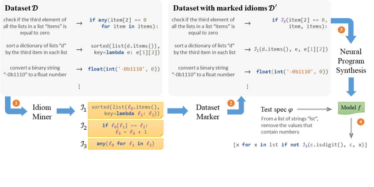
0-1=dj0-1=If0-1=0-1=Compare0-1=0-1=Subscript0-1=0-1=$\ell_{0}\colon\texttt{list}$0-1=Index0-1=0-1=$\ell_{1}\colon\texttt{int}$0-1=Eq0-1=Num0-1=0-1=$\ell_{2}$0-1=stmt*0-1=0-1=Assign0-1=0-1=$\ell_{3}$0-1=BinOp0-1=0-1=$\ell_{3}$0-1=Add0-1=Num0-1=0-1=10-1=…

Figure 1: Top: An overview of Patois.A miner \raisebox{-.8pt}{\small1}⃝ extracts common idioms from the programs in a given dataset.All the idiom occurrences in the dataset programs are \raisebox{-.8pt}{\small2}⃝ marked as optional alternative grammar operators.The dataset with marked occurrences is used to \raisebox{-.8pt}{\small3}⃝ train a neural generative model.At inference time, the model \raisebox{-.8pt}{\small4}⃝ generates programs with named idioms, which are inlined beforeprogram execution.Note that idioms may have named subexpressions, may repeat, and may occur at any program level.For clarity, we typeset idioms using function-like syntax ${\mathcal{I}_{j}}(\ell_{1},\dots,\ell_{k})$ in this paper, although they are actually represented as AST fragments with no syntax.
Bottom: AST fragment representation of the idiom $\mathcal{I}_{2}$ in Python.Here sans-serif nodes are fixed non-terminals, monospaced nodes are fixed terminals,and nodes are named arguments.

2 Background

Program Synthesis

We consider the following formulation of the program synthesis problem.Assume an underlying programming language $\dsl$ of programs.Each program $P\in\dsl$ can be represented either as a sequence $y_{1}\cdots y_{|P|}$ of its tokens, or,equivalently, as an abstract syntax tree (AST) $T$ parsed according to the context-free grammar (CFG)$\mathcal{G}$ of the language $\dsl$.The goal of a program synthesis model $f\colon\spec\mapsto P$ is to generate a program $P$ thatmaximizes the conditional probability $\Pr\left(P\mid\spec\right)$ the most likely program giventhe specification.We also assume a training set $\mathcal{D}=\left\{\langle\spec_{j},P_{j}\rangle\right\}_{j=1}^{|\mathcal{D}|}$, sampledfrom an unknown true distribution $\mathfrak{D}$, from whichwe wish to estimate the conditional probability $\Pr\left(P\mid\spec\right)$.In this work, we consider general-purpose programming languages $\dsl$ with a known context-free grammar $\mathcal{G}$such as Python and SQL.Each specification $\spec$ is represented asa natural language task description, a sequence of words $X=x_{1}\cdots x_{|X|}$(although the Patois synthesizer can be conditioned on any other type of incomplete spec).In principle, we do not impose any restrictions on the generative model $f$ apart from it beingable to emit syntactically valid programs.However, as we detail in Section 4, the Patois framework is most easily implemented on top ofstructural generative models such as sequence-to-tree models [38] and graph neuralnetworks [21, 7].

Code Idioms

Following Allamanis and Sutton [2], we define code idioms as fragments $\mathcal{I}$ of valid ASTs $T$ in theCFG $\mathcal{G}$, trees of nonterminals and terminals from $\mathcal{G}$ that may occur as subtrees of valid parse treesfrom $\mathcal{G}$.The grammar $\mathcal{G}$ extended with a set of idiom fragments forms a tree substitution grammar (TSG).We also associate a non-unique label $\ell$ with each nonterminal leaf in every idiom, and requirethat every instantiation of an idiom $\mathcal{I}$ must have its identically-labeled nonterminals instantiated to identicalsubtrees.This enables the role of idioms as subroutines, where labels act as “named arguments” in the “body” of anidiom.See Figure 1 for an example.

3 Mining Code Idioms

The first step of Patois is obtaining a set of frequent and useful AST fragments as code idioms.The trade-off between frequency and usefulness is crucial: it is trivial to mine commonly occurring shortpatterns, but they are often meaningless [1].Instead, we employ and extend the methodology of Allamanis et al. [3] and frame idiom mining as a nonparametericBayesian problem.We represent idiom mining as inference over probabilistic tree substitution grammars (pTSG).A pTSG is a probabilistic context-free grammar extended with production rules that expand to a whole AST fragmentinstead of a single level of symbols [8, 29].The grammar $\mathcal{G}$ of our original language $\dsl$ induces a pTSG $\mathcal{G}_{0}$ with no fragment rules and withchoice probabilities estimated from the corpus $\mathcal{D}$.To construct a pTSG corresponding to the extension of $\dsl$ with common tree fragments representing idioms,we define a distribution $\mathfrak{G}$ over pTSGs as follows.We first choose a Pitman-Yor process [36] as a prior distribution $\mathfrak{G}_{0}$ over pTSGs.It is a nonparameteric process that has proven to be effective for mining code idioms in prior work thanks to itsmodeling of production choices as a Zipfian distribution (in other words, it implements the desired “rich get richer”effect, which encourages a smaller number of larger and more common idioms).

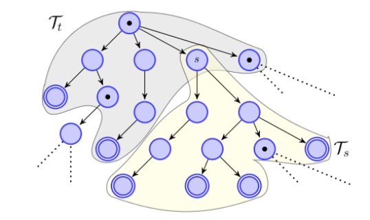
Figure 2: MCMC sampling for an AST (figure from [2]).Dots show the inferred nodes where the AST is split into fragments.

Formally, it is a “stick-breaking” process [31] that defines $\mathfrak{G}_{0}$ as adistribution for each set of idioms $\widetilde{\mathcal{I}}_{N}$ rooted at a nonterminal symbol $N$ as

$$\Pr(\mathcal{I}\in\widetilde{\mathcal{I}}_{N})\bydef\sum_{k=0}^{\infty}\pi_{k}\,\delta\left(\mathcal{I}=\mathcal{I}_{k}\right),\quad\mathcal{I}_{k}\sim\mathcal{G}_{0}$$

$$\pi_{k}\bydef u_{k}\prod_{j=1}^{k-1}(1-u_{j}),\ u_{k}\sim\mathrm{Beta}\left(1-d,\,\alpha+kd\right)$$

where $\delta(\cdot)$ is the delta function, and $\alpha$, $d$ are hyperparameters.See Allamanis et al. [3] for details.Patois uses $\mathfrak{G}_{0}$ to compute a posterior distribution $\mathfrak{G}_{1}=\Pr\left(\mathcal{G}_{1}\mid T_{1},\dots,T_{N}\right)$ using Bayes’ rule, where $T_{1},\dots,T_{N}$ are concrete AST fragments in the training set$\mathcal{D}$.As this calculation is computationally intractable, we approximate it using type-based MCMC [23].At each iteration $t$ of the MCMC process, Patois generates a pTSG $\mathcal{G}_{t}$ whose distribution approaches$\mathfrak{G}_{1}$ as $t\to\infty$.It works by sampling splitting points for each AST $T$ in the corpus $\mathcal{D}$, which by construction definea set of fragments constituting $\mathcal{G}_{t}$ (see Figure 2).The split probabilities of this Gibbs sampling are set in a way that incentivizes merging adjacent tree fragments thatoften cooccur in $\mathcal{D}$.The final idioms are then extracted from the pTSG obtained at the last MCMC iteration.While the Pitman-Yor process helps avoid overfitting the idioms to $\mathcal{D}$, not all sampled idioms are useful forsynthesis.Thus we rank and filter the idioms before using them in the training.In this work, we reuse two ranking functions defined by Allamanis et al. [3]:

$$\mathsf{Score_{Cov}}\left(\mathcal{I}\right) \bydef\text{coverage}=\mathsf{count}(T\in\mathcal{D}\mid\mathcal{I}\in T)$$

$$\mathsf{Score_{CXE}}\left(\mathcal{I}\right) \bydef\text{coverage}\cdot\text{cross-entropy gain}=\frac{\mathsf{count}(T\in\mathcal{D}\mid\mathcal{I}\in T)}{|\mathcal{D}|}\cdot\frac{1}{|\mathcal{I}|}\log\frac{\Pr_{\mathfrak{G}_{1}}(\mathcal{I})}{\Pr_{\mathfrak{G}_{0}}(\mathcal{I})}$$

and also filter out any terminal idioms (those that do not contain any named arguments $\ell$).We conclude with a brief analysis of computational complexity of idiom mining.Every iteration of the MCMC sampling traverses the entire dataset $\mathcal{D}$ once to sample the random variables thatdefine the splitting points in each AST.When run for $M$ iterations, the complexity of idiom mining is $\order{M\cdot\sum_{T\in\mathcal{D}}|T|}$.Idiom ranking adds an additional step with complexity $\order{|\widetilde{\mathcal{I}}|\log|\widetilde{\mathcal{I}}|}$ where$\widetilde{\mathcal{I}}$ is the set of idioms obtained at the last iteration.In our experiments (detailed in Section 5) we set $M=10$, and the entire idiom mining takes less than 10minutes on a dataset of $|\mathcal{D}|\approx\numprint{10000}$ ASTs.

4 Using Idioms in Program Synthesis

Given a set of common idioms $\widetilde{\mathcal{I}}=\{\mathcal{I}_{1},\dots,\mathcal{I}_{N}\}$ mined by Patois,we now aim to learn a synthesis model $f$ that emits whole idioms $\mathcal{I}_{j}$ as atomic actions instead ofindividual AST nodes that comprise $\mathcal{I}_{j}$.Achieving this involves two key challenges.First, since idioms are represented as AST fragments without concrete syntax, Patois works best when thesynthesis model $f$ is structural, it generates the program AST instead of its syntax.Prior work [38, 40, 7] also showed that tree- and graph-based code generation modelsoutperform sequence-to-sequence models, and thus we adopt a similar architecture in this work.Second, exposing the model $f$ to idiom usage patterns is not obvious.One approach could be to extend the grammar with new named operators $\mathsf{op}_{\mathcal{I}}(\ell_{1},\dots,\ell_{k})$ foreach idiom $\mathcal{I}$, replace every occurrence of $\mathcal{I}$ with $\mathsf{op}_{\mathcal{I}}$ in the data, andtrain the synthesizer on the rewritten dataset.However, this would not allow $f$ to learn from the idiom definitions (bodies).In addition, idiom occurrences often overlap, and any deterministic rewriting strategy would arbitrarily discard someoccurrences from the corpus, thus limiting the model’s exposure to idiom usage.In our experiments, we found that greedy rewriting discarded as many as $75\%$ potential idiom occurrences from thedataset.Therefore, a successful training strategy must preserve all occurrences and instead let the model learn arewriting strategy that optimizes end-to-end synthesis accuracy.To this end, we present a novel training setup for code generation that encourages the model to choose the mostuseful subset of idioms and the best representation of each program in terms of the idioms.It works by 1 marking occurrences of the idioms $\widetilde{\mathcal{I}}$ in the training set $\mathcal{D}$ 2 at training time, encouraging the model to emit either the whole idiom or itsbody for every potential idiom occurrence in the AST 3 at inference time, replacing the model’s state after emitting an idiom $\mathcal{I}$ with the state the model wouldhave if it had emitted $\mathcal{I}$’s body step by step.

4.1 Model Architecture

The synthesis model $f$ of Patois combines a spec encoder $f_{\text{enc}}$ and an AST decoder $f_{\text{dec}}$,following the formulation of Yin and Neubig [38].The encoder $f_{\text{enc}}$ embeds the NL specification $X=x_{1}\cdots x_{n}$ intoword representations $\hat{X}=\vect{\hat{x}}_{1}\cdots\vect{\hat{x}}_{n}$.The decoder $f_{\text{dec}}$ uses an LSTM to model the sequential generation of the AST in the depth-first order,wherein each timestep $t$ corresponds to an action $a_{t}$ — either (a) expanding a productionfrom the grammar, (b) expanding an idiom, or (c) generating a terminal token.Thus, the probability of generating an AST $T$ given $\hat{X}$ is

$$\Pr(T\mid\hat{X})=\prod\nolimits_{t}\Pr\bigl{(}a_{t}\mid T_{t},\hat{X}\bigr{)}$$ (1)

where $a_{t}$ is the action taken at timestep $t$, and $T_{t}$ is the partial AST generated before $t$.The probability $\Pr(a_{t}\mid T_{t},\hat{X})$ is computed from the decoder’s hidden state $\vect{h}_{t-1}$depending on $a_{t}$.

Production Actions

For actions $a_{t}=\textsc{ApplyRule}[R]$ corresponding to expanding production rules $R\in\mathcal{G}$ from the original CFG $\mathcal{G}$, we compute the probability$\Pr(a_{t}\mid T_{t},\hat{X})$ by encoding the current partial AST structure similarly to Yin and Neubig [38].Specifically, we compute the new hidden state as$\vect{h}_{t}=f_{\text{LSTM}}\left([\vect{a}_{t-1}\conc\vect{c}_{t}\conc\vect{h}_{p_{t}}\conc\vect{a}_{p_{t}}\conc\vect{n}_{f_{t}}],\ \vect{h}_{t-1}\right)$where $\vect{a}_{t-1}$ is the embedding of the previous action, $\vect{c}_{t}$ is the result of soft attention applied tothe spec embeddings $\hat{X}$ as per Bahdanau et al. [4], $p_{t}$ is the timestep corresponding to expanding theparent AST node of the current node, and $\vect{n}_{f_{t}}$ is the embedding of the current node type.The hidden state $\vect{h}_{t}$ is then used to compute probabilities of the syntactically appropriate production rules$R\in\mathcal{G}$:

$$\Pr(a_{t}=\textsc{ApplyRule}[R]\mid T_{t},\hat{X})=\mathsf{softmax}_{R}\left(g(\vect{h}_{t})\right)$$ (2)

where $g(\cdot)$ is a 2-layer MLP with a $\mathsf{tanh}$ non-linearity.

Terminal Actions

For actions$a_{t}=\textsc{GetToken}[y]$, we compute the probability $\Pr(a_{t}\mid T_{t},\hat{X})$by combining a small vocabulary $\mathcal{V}$ of tokens commonly observed in the training data with acopying mechanism [24, 30] over the input $X$ to handle UNK tokens.Specifically, we learn twofunctions $p_{\text{gen}}(\vect{h}_{t})$ and $p_{\text{copy}}(\vect{h}_{t},X)$ such that$p_{\text{gen}}$ produces a score for each vocabulary token $y\in\mathcal{V}$and $p_{\text{copy}}$ computes a score forcopying the token $y$ from the input.The scores are then normalized across the entries corresponding to the same constant, as in [38, 7].

4.2 Training to Emit Idioms

As discussed earlier, training the model to emit idioms presents computational and learning challenges.Ideally, we would like to extend Eq. 1 to maximize

$$\mathcal{J}=\sum_{\tau\in\mathcal{T}}\prod_{i=1}^{|\tau|}\Pr(a_{\tau_{i}}\mid T_{\tau_{i}},\hat{X})$$ (3)

where $\mathcal{T}$ is a set of different action traces that may produce the output AST $T$.The traces $\tau\in\mathcal{T}$ differ only in their possible choices of idiom actions$\textsc{ApplyRule}[\mathsf{op}_{\mathcal{I}}]$ that emit some tree fragments of $T$ in a single step.However, computing Eq. 3 is intractable because idiom occurrences overlap and cause combinatorialexplosion in the number of traces $\mathcal{T}$.Instead, we apply Jensen’s inequality and maximize a lower bound:

$$\log\mathcal{J}=\log\sum_{\tau\in\mathcal{T}}\prod_{i=1}^{|\tau|}\Pr(a_{\tau_{i}}\mid T_{\tau_{i}},\hat{X})\geq\log(|\mathcal{T}|)+\frac{1}{|\mathcal{T}|}\sum_{\tau\in\mathcal{T}}\sum_{i=1}^{|\tau|}\log\Pr(a_{\tau_{i}}\mid T_{\tau_{i}},\hat{X})$$ (4)

Let $A(T_{t})=\{a^{*}_{t}\}\cup I(T_{t})$ be the set of all valid actions to expand theAST $T_{t}$ at timestep $t$.Here $a^{*}_{t}$ is the action from the original action trace that generates $T$ using the original CFG and$I(T_{t})$ is the set of idiom actions $\textsc{ApplyRule}[\mathsf{op}_{\mathcal{I}}]$ also applicable at the node to be expandedin $T_{t}$.Let $c(\mathcal{T},t)$ also denote the number of traces $\tau\in\mathcal{T}$ that admit an action choice for the AST$T_{t}$ from the original action trace.Since each action $a\in A(T_{t})$ occurs in the sum in Eq. 4 with probability${c(\mathcal{T},t)}\,\big{/}\,{|A(T_{t})|}$, we canrearrange this sum over traces as a sum over timesteps of the original trace:

$$\frac{1}{|\mathcal{T}|}\sum_{\tau\in\mathcal{T}}\sum_{i=1}^{|\tau|}\log\Pr(a_{\tau_{i}}\mid T_{\tau_{i}},\hat{X})=\frac{1}{|\mathcal{T}|}\sum_{t}\sum_{a\in A(T_{t})}\frac{c(\mathcal{T},t)}{|A(T_{t})|}\log\Pr(a\mid T_{\tau_{i}},\hat{X})$$

$$\quad=\sum_{t}\frac{1}{|A(T_{t})|}\sum_{a\in A(T_{t})}\frac{c(\mathcal{T},t)}{|\mathcal{T}|}\log\Pr(a\mid T_{\tau_{i}},\hat{X})=\operatorname*{\mathbb{E}}_{T_{t}\sim\mathcal{T}}\frac{1}{|A(T_{t})|}\sum_{a\in A(T_{t})}\log\Pr(a\mid T_{\tau_{i}},\hat{X})$$

$$\quad\approx\sum_{t}\frac{1}{|A(T_{t})|}\Bigl{[}\log\Pr(a^{*}_{t}\mid T_{t},\hat{X})+\sum_{\mathclap{\mathcal{I}\in M(T_{t})}}\log\Pr(a_{t}=\textsc{ApplyRule}[\mathsf{op}_{\mathcal{I}}]\mid T_{t},\hat{X})\Bigr{]}$$ (5)

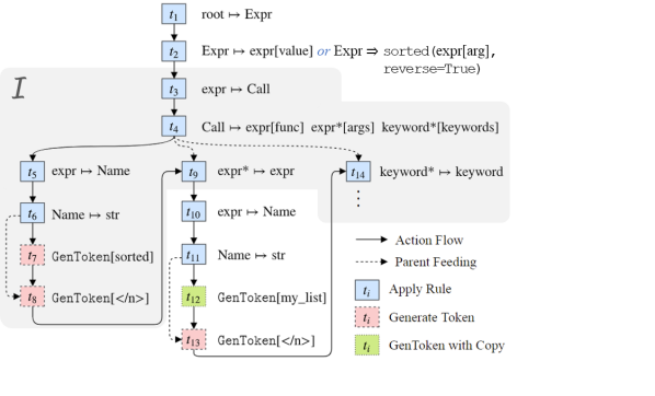
Figure 3: Decoding the AST sorted(my_list,reverse=True), figure adapted from[38].Suppose an idiom$\mathcal{I}=\$sorted( , reverse=True)is mined and added as an operator $\mathsf{op}_{\mathcal{I}}(\ell)$ to the grammar.At training time, Patois adjusts the cross-entropy objective at timestep $t_{2}$ to additionally allow$\mathsf{op}_{\mathcal{I}}$ as a valid production, with no change to further decoding.At inference time, if decoder emits an action $a_{t_{2}}=\textsc{ApplyRule}[\mathsf{op}_{\mathcal{I}}]$, Patois unrolls$\mathcal{I}$ on the fly by teacher-forcing the shaded portion of the AST generation.

In the last step of Section 4.2, we approximate the expectation over ASTs randomly drawn from alltraces $\mathcal{T}$ using only the original trace (containing all possible $T_{t}$) as a Monte Carlo estimate.Intuitively, at each timestep during training we encourage the model to emit either the original AST action forthis timestep or any applicable idiom that matches the AST at this step, with no penalty to either choice.However, to avoid the combinatorial explosion, we only teacher-force the original generation trace (not the idiombodies), thus optimizing the bound in Section 4.2.Figure 3 illustrates this optimization process on an example.At inference time, whenever the model emits an $\textsc{ApplyRule}[\mathsf{op}_{\mathcal{I}}]$ action, we teacher-force the body of$\mathcal{I}$ by substituting the embedding of the previous action $\vect{a}_{t-1}$ with embedding of the previousaction in the idiom definition, thus emulating the tree fragment expansion.Outside the bounds of $\mathcal{I}$ (within the hole subtrees of $\mathcal{I}$) we use the actual $\vect{a}_{t-1}$ as usual.

5 Evaluation

Datasets

We evaluate Patois on two semantic parsing datasets:Hearthstone [24]and Spider [41].Hearthstone is a dataset of 665 card descriptions from the tradingcard game of the same name, along with the implementations of their effects in Python using the game APIs.The descriptions act as NL specs $X$, and are on average 39.1 words long.Spider is a dataset of 10,181 questions describing 5,693unique SQL queries over 200 databases with multiple tables each.Each question pertains to a particular database, whose schema is given to the synthesizer.Database schemas do not overlap between the train and test splits, thus challenging the model to generalize acrossdifferent domains.The questions are on average 13 words long and databases have on average 27.6 columns and 8.8 foreign keys.

Implementation

We mine the idioms using the training split of each dataset.Thus Patois cannot indirectly overfit to the test set by learning its idioms, but it also cannot generalize beyond theidioms that occur in the training set.We run type-based MCMC (Section 3) for 10 iterations with $\alpha=5$ and $d=\numprint{0.5}$.After ranking (with either $\mathsf{Score_{COV}}$ or $\mathsf{Score_{CXE}}$) and filtering, we use $K$top-ranked idioms to train the generative model.We ran ablation experiments with $K\in\left\{10,20,40,80\right\}$.As described in Section 4, for all our experiments we used a tree-based decoder witha pointer mechanism as the synthesizer $f$, which we implemented in PyTorch [27].For the Hearthstone dataset, we use a bidirectional LSTM [16] to implement the description encoder $\hat{X}=f_{\text{enc}}(X)$, similarly to Yin and Neubig [38].The word embeddings $\vect{\hat{x}}$ and hidden LSTM states $\vect{h}$ have dimension 256.The models are trained using the Adadelta optimizer [42] with learning rate $1.0$, $\rho=0.95$,$\varepsilon=\numprint{e-6}$ for up to 2,600 steps with a batch size of 10.For the Spider dataset,word embeddings $\vect{\hat{x}}$ have dimension 300, and hidden LSTM states $\vect{h}$ have dimension 256.The models are trained using the Adam optimizer [20] with $\beta_{1}=0.9$, $\beta_{2}=0.999$,$\varepsilon=\numprint{e-9}$ for up to 40,000 steps with a batch size of 10.The learning rate warms up linearly up to 2.5×10^-4 during the first 2,000 steps,and then decays polynomially by $\left(1-t/T\right)^{-0.5}$ where $T$ is the total number of steps.Each model configuration is trained on one NVIDIA GTX 1080 Ti GPU.The Spider tasks additionally include the database schema as an input in the description.We follow a recent approach of embedding the schema using relation-aware self-attention within theencoder [34].Specifically, we initialize a representation for each column, table, and word in the question, and then update theserepresentations using 4 layers of relation-aware self-attention [32] using a graph that describes therelations between columns and tables in the schema.See Section A in the appendix for more details about the Spider schema encoder.

5.1 Experimental Results

In each configuration, we compare the performance of equivalent trained models on the same dataset with and withoutidiom-based training of Patois.For fairness, we show the performance of the same decoder implementation described in Section 4.1 as abaseline rather than the state-of-the-art results achieved by different approaches from the literature.Thus, our baseline is the decoder described in Section 4.1 trained with a regular cross-entropy objectiverather than the Patois objective in Section 4.2.Following prior work, we evaluate program generation as a semantic parsing task, and measure(i) exact match accuracy and BLEU scores for Hearthstone and(ii) exact match accuracy of program sketches for Spider.

Table 2: Ablation tests on the Hearthstone dev set.

Model	$\bm{K}$	[t]1.08cmExact match	[t]1.08cmSentence BLEU	[t]1.08cmCorpus BLEU
Baseline decoder	—	0.197	0.767	0.763
Patois, $\mathsf{Score_{Cov}}$	10	0.151	0.781	0.785
	20	0.091	0.745	0.745
	40	0.167	0.765	0.764
	80	0.197	0.780	0.774
Patois, $\mathsf{Score_{CXE}}$	10	0.151	0.780	0.783
	20	0.167	0.787	0.782
	40	0.182	0.773	0.770
	80	0.151	0.771	0.768

Table 3: Ablation tests on the Spider dev set.

Model	$\bm{K}$	Exact match
Baseline decoder	—	0.395
Patois, $\mathsf{Score_{Cov}}$	10	0.394
	20	0.379
	40	0.395
	80	0.407
Patois, $\mathsf{Score_{CXE}}$	10	0.368
	20	0.382
	40	0.387
	80	0.416

Tables 3 and 3 show our ablation analysis of different configurations of Patois on theHearthstone and Spider dev sets, respectively.Table 4 shows the test set results of the best model configuration for Hearthstone(the test instances for the Spider dataset are unreleased).

Table 4: Test set results on Hearthstone (using the best configurations on the dev set).

Model	[t]1.08cmExact match	[t]1.08cmSentence BLEU	[t]1.08cmCorpus BLEU
Baseline	0.152	0.743	0.723
Patois	0.197	0.780	0.766

As the results show, small numbers of idioms do not significantly change the exact match accuracy but improve BLEUscore, and $K=80$ gives a significant improvement in both the exact match accuracy and BLEU scores.The improvement is even more pronounced on the test set with $4.5\%$ improvement in exact match accuracy and morethan 4 BLEU points, which shows that mined training set idioms generalize well to the whole data distribution.As mentioned above, we compare only to the same baseline architecture for fairness, but Patois could also be easilyimplemented on top of the structural CNN decoder of Sun et al. [35], the current state of the art on theHearthstone dataset.

⬇

super().__init__( , ,

CHARACTER_CLASS. ,

CARD_RARITY. , )

⬇

copy.copy( )

 

⬇

def __init__(self):

⬇

INTERSECT EXCEPT

 

Figure 4: Five examples of commonly used idioms from the Hearthstone and Spider datasets.

Figure 4 shows some examples of idioms that were frequently used by the model.On Hearthstone, the most popular idioms involve common syntactic elements (class and function definitions) anddomain-specific APIs commonly used in card implementations (CARD_RARITY enumerations orcopy.copy calls).On Spider, they capture the most common combinations of SQL syntax, such as a SELECT querywith a single COUNT column and optional INTERSECT orEXCEPT clauses.Notably, popular idioms are also often big: for instance, the first idiom in Figure 4expands to a tree fragment with more than 20 nodes.Emitting it in a single step vastly simplifies the decoding process.

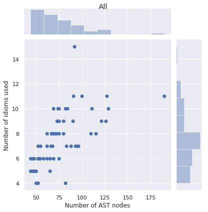
Figure 5: The distribution of used idioms in the inferred ASTs on the Hearthstone test set.Left: in the ASTs exactly matched with ground truth; Right: all ASTs.

We further conducted qualitative experiments to analyze actual idiom usage by Patois on the Hearthstone test set.Figure 5 shows the distribution of idioms used in the inferred (not ground truth) ASTs.A typical program involves 7 idioms on average, or 6 for the programs that exactly match the ground truth.Despite the widespread usage of idioms, not all of the mined idioms $\widetilde{\mathcal{I}}$ were useful: only 51 out of$K=80$ idioms appear in the inferred ASTs.This highlights the need for an end-to-end version of Patois where idiom mining would be directly optimized to benefitsynthesis.

6 Related Work

Program synthesis & Semantic parsing

Program synthesis from natural language and input-output examples has a long history in Programming Languages (PL) andMachine Learning (ML) communities (see Gulwani et al. [15] for a survey).When an input specification is limited to natural language, the resulting problem can be considered semanticparsing [22].There has been a lot of recent interest in applying recurrent sequence-based and tree-based neural networks to semanticparsing [38, 21, 11, 18, 40].These approaches commonly use insights from the PL literature, such as grammar-based constraints to reduce the searchspace, non-deterministic training oracles to enable multiple executable interpretations of intent, and supervision fromprogram execution.They typically either supervise the training on one or more golden programs, or use reinforcement learning to supervisethe training from a neural program execution result [26].Our Patois approach is applicable to any underlying neural semantic parsing model, as long as it is supervised by acorpus of golden programs.It is, however, most easily applicable to tree-based and graph-based models, which directly emit the AST of the targetprogram.In this work we have evaluated Patois as applied on top of the sequence-to-tree decoder of Yin and Neubig [38], andextended it with a novel training regime that teaches the decoder to emit idiom operators in place of the idiomaticcode fragments.

Sketch generation

Two recent works [12, 25] learn abstractions of the target program to compress and abstract thereasoning process of a neural synthesizer.Both of them split the generation process into sketch generation and sketch completion, wherein the firststage emits a partial tree/sequence (a sketch of the program) and the second stage fills in the holes in thissketch.While sketch generation is typically implemented with a neural model, sketch completion can be either a different neuralmodel or a combinatorial search.In contrast to Patois, both works define the grammar of sketches manually by a deterministic program abstractionprocedure and only allow a single top-level sketch for each program.In addition, an earlier work of Bošnjak et al. [6] also formulates program synthesis as sketch completion,but in their work program sketches are manually provided rather than learned.In Patois, we learn the abstractions (code idioms) automatically from a corpus and allow them to appearanywhere in the program, as is common in real-life programming.

Learning abstractions

Recently, Ellis et al. [13] developed an Explore, Compress & Compile (EC²) framework for automaticallylearning DSLs for program synthesis from I/O examples (such as the DSLs used by FlashFill [14] andDeepCoder [5]).The workflow of EC² is similar to Patois, with three stages:(a) learn new DSL subroutines from a corpus of tasks,(b) train a recognition model that maps a task specification to a distribution over DSL operatorsas in DeepCoder [5], and(c) use these operators in a program synthesizer.Patois differs from EC² in three aspects:(i) we assume a natural language specification instead of examples,(ii) to handle NL specifications, our synthesizer is a neural semantic parser instead of enumerativesearch, and(iii) most importantly, we discover idioms that compress general-purpose languages instead ofextending DSLs.Unlike for inductive synthesis DSLs such as FlashFill, the existence of useful DSL abstractions forgeneral-purpose languages is not obvious, and our work is the first to demonstrate them.Concurrently with this work, Iyer et al. [17] developed a different approach of learning code idioms forsemantic parsing.They mine the idioms using a variation of byte-pair encoding (BPE) compression extended to ASTs and greedilyrewrite all the dataset ASTs in terms of the found idioms for training.While the BPE-based idiom mining is more computationally efficient than non-parametric Bayesian inference of Patois,introducing ASTs greedily tends to lose information about overlapping idioms, which we address in Patois using ournovel training objective described in Section 4.2.As described previously, our code idiom mining is an extension of the procedure developed byAllamanis et al. [2, 3].They are the first to use the tree substitution grammar formalism and Bayesian inference to find non-trivial commonidioms in a corpus of code.However, their problem formalization does not involve any application for the learned idioms beyond their explanatorypower.

7 Conclusion

Semantic parsing, or neural program synthesis from natural language, has made tremendous progress over the past years,but state-of-the-art models still struggle with program generation at multiple levels of abstraction.In this work, we present a framework that allows incorporating learned coding patterns from a corpus into the vocabularyof a neural synthesizer, thus enabling it to emit high-level or low-level program constructsinterchangeably at each generation step.Our current instantiation, Patois, uses Bayesian inference to mine common code idioms, and employs anovel nondeterministic training regime to teach a tree-based generative model to optionally emit whole idiomfragments.Such dataset abstraction using idioms improves the performance of neural program synthesis.Patois is only the first step toward learned abstractions in program synthesis.While code idioms often correlate with latent semantic conceptsand our training regime allows the model to learn which idioms to use and in which context,our current method does not mine them with the intent to directly optimize their usefulness for generation.In future work, we want to alleviate this by jointly learning the mining and synthesis models, thusoptimizing the idioms’ usefulness for synthesis by construction.We also want to incorporate program semantics into the idiom definition, such as data flow patterns ornatural language phrases from task specs.

Appendix A Encoder for Spider dataset

Table 5: Description of edge types present in the directed graph created to represent the schema. An edge exists from node $x$ to node $y$ if the pair fulfills one of the descriptions listed in the table, with the corresponding label. Otherwise, no edge exists from $x$ to $y$.

Type of $x$	Type of $y$	Edge label	Description
Column	Column	Same-Table	$x$ and $y$ belong to the same table.
		Foreign-Key-Col-F	$x$ is a foreign key for $y$.
		Foreign-Key-Col-R	$y$ is a foreign key for $x$.
Column	Table	Primary-Key-F	$x$ is the primary key of $y$.
		Belongs-To-F	$x$ is a column of $y$ (but not the primary key).
Table	Column	Primary-Key-R	$y$ is the primary key of $x$.
		Belongs-To-R	$y$ is a column of $x$ (but not the primary key).
Table	Table	Foreign-Key-Tab-F	Table $x$ has a foreign key column in $y$.
		Foreign-Key-Tab-R	Same as above, but $x$ and $y$ are reversed.
		Foreign-Key-Tab-B	$x$ and $y$ have foreign keys in both directions.

In the Spider dataset, each entry contains a question along with a database schema, containing tables and columns.We will use the following notation:

• $c_{i}$ for each column in the schema. Each column contains words $c_{i,1},\cdots,c_{i,|c_{i}|}$.

• $t_{i}$ for each table in the schema. Each table contains words $t_{i,1},\cdots,t_{i,|t_{i}|}$.

• $q$ for the input question. The question contains words $q_{1},\cdots,q_{|q|}$.

A.1 Encoding the Schema as a Graph

We begin by representing the database schema using a directed graph $\mathcal{G}$, where each node and edge has a label.We represent each table and column in the schema as a node in this graph, labeled with the words in the name;for columns, we prepend the type of the column to the label.For each pair of nodes $x$ and $y$ in the graph, Table 5 describes when there exists an edge from $x$ to $y$ and the label it should have.

A.2 Initial Encoding of the Input

We now obtain an initial representation for each of the nodes in the graph, as well as for the words in the input question.Formally, we perform the following:

$$(\mathbf{c}_{i,0}^{\text{fwd}},\mathbf{c}_{i,0}^{\text{rev}}),\cdots,(\mathbf{c}_{i,|c_{i}|}^{\text{fwd}},\mathbf{c}_{i,|c_{i}|}^{\text{rev}}) =\text{BiLSTM}_{\text{Column}}(c_{i}^{\text{type}},c_{i,1},\cdots,c_{i,|c_{i}|});\quad\mathbf{c}_{i}^{\text{init}}=\text{Concat}(\mathbf{c}_{i,|c_{i}|}^{\text{fwd}},\mathbf{c}_{i,0}^{\text{rev}})$$

$$(\mathbf{t}_{i,1}^{\text{fwd}},\mathbf{t}_{i,1}^{\text{rev}}),\cdots,(\mathbf{t}_{i,|t_{i}|}^{\text{fwd}},\mathbf{t}_{i,|t_{i}|}^{\text{rev}}) =\text{BiLSTM}_{\text{Table}}(t_{i,1},\cdots,t_{i,|t_{i}|});\quad\mathbf{t}_{i}^{\text{init}}=\text{Concat}(\mathbf{t}_{i,|c_{i}|}^{\text{fwd}},\mathbf{t}_{i,1}^{\text{rev}})$$

$$(\mathbf{q}_{1}^{\text{fwd}},\mathbf{q}_{1}^{\text{rev}}),\cdots,(\mathbf{q}_{|q|}^{\text{fwd}},\mathbf{q}_{|q|}^{\text{rev}}) =\text{BiLSTM}_{\text{Question}}(q_{1},\cdots,q_{|q|});\quad\mathbf{q}_{i}^{\text{init}}=\text{Concat}(\mathbf{q}_{i}^{\text{fwd}},\mathbf{q}_{i}^{\text{rev}})$$

where each of the BiLSTM functions first lookup word embeddings for each of the input tokens.The LSTMs do not share any parameters with each other.

A.3 Relation-Aware Self-Attention

At this point, we have representations $\mathbf{c}_{i}^{\text{init}}$, $\mathbf{t}_{i}^{\text{init}}$, and $\mathbf{q}_{i}^{\text{init}}$.Now, we would like to imbue these representations with the information in the schema graph.We use a form of self-attention [37] that is relation-aware [33] to achieve this goal.In one step of relation-aware self-attention, we begin with an input $\mathbf{x}$ of $n$ elements (where $x_{i}\in\mathbb{R}^{d_{x}}$) and transform each $x_{i}$ into $y_{i}\in\mathbb{R}^{d_{z}}$.We follow the formulation described in Shaw et al. [33]:

$$e_{ij}^{(h)} =\frac{x_{i}W_{Q}^{(h)}(x_{j}W_{K}^{(h)}+\mathbf{\color[rgb]{1,0,0}r_{ij}^{K}})^{T}}{\sqrt{d_{z}/H}};\quad\alpha_{ij}^{(h)}=\frac{\exp(e_{ij}^{(h)})}{\sum_{l=1}^{n}\exp(e_{il}^{(h)})}$$

$$z_{i}^{(h)} =\sum_{j=1}^{n}\alpha_{ij}^{(h)}(x_{j}W_{V}^{(h)}+\mathbf{\color[rgb]{1,0,0}r_{ij}^{V}});\quad z_{i}=\text{Concat}(z_{i}^{(0)},\cdots,z_{i}^{(H)})$$

$$\tilde{y}_{i} =\text{LayerNorm}(x_{i}+z_{i});\quad y_{i}=\text{LayerNorm}(\tilde{y}_{i}+\text{FC}(\text{ReLU}(\text{FC}(\tilde{y}_{i})))$$

The $r_{ij}$ terms encode the relationship between the two elements $x_{i}$ and $x_{j}$ in the input.We explain how we obtain $r_{ij}$ in the next part.For the application within the Spider encoder, we first construct the input $x$ of $|c|+|t|+|q|$ elements using $\mathbf{c}_{i}^{\text{init}}$, $\mathbf{t}_{i}^{\text{init}}$, and $\mathbf{q}_{i}^{\text{init}}$:

$$x=(\mathbf{c}_{1}^{\text{init}},\cdots,\mathbf{c}_{|c|}^{\text{init}},\mathbf{t}_{1}^{\text{init}},\cdots,\mathbf{t}_{|t|}^{\text{init}},\mathbf{q}_{1}^{\text{init}},\cdots,\mathbf{q}_{|q|}^{\text{init}}).$$

We then apply a stack of 4 relation-aware self-attention layers.We set $d_{z}=d_{x}$ to facilitate this stacking.The weights of the encoder layers are not tied; each layer has its own set of weights.We define a discrete set of possible relation types, and map each type to an embedding to obtain $r_{ij}^{V}$ and $r_{ij}^{K}$.We need a value of $r_{ij}$ for every pair of elements in $x$.If $x_{i}$ and $x_{j}$ both correspond to nodes in $\mathcal{G}$ (i.e. each is either a column or table) with an edge from $x_{i}$ to $x_{j}$, then we use the label on that edge (possibilities listed in Table 5).However, this is not sufficient to obtain $r_{ij}$ for every pair of $i$ and $j$.In the graph we created for the schema, we have no nodes corresponding to the question words;not every pair of nodes in the graph has an edge between them (the graph is not complete);and we have no self-edges (for when $i=j$).As such, we add more types beyond what is defined in Table 5:

• $x_{i}\in$ question, $x_{j}\in$ question:Question-Dist-$d$, where $d=\text{clip}(j-i,D)$; $\text{clip}(a,D)=\max(-D,\min(D,a))$. We use $D=2$.

• If $i=j$, then Column-Identity or Table-Identity.

• $x_{i}\in$ question, $x_{j}\in\text{column}\cup\text{table}$; or $x_{i}\in\text{column}\cup\text{table}$, $x_{j}\in$ question:
  Question-Column, Question-Table, Column-Question or Table-Questiondepending on the type of $x_{i}$ and $x_{j}$.

• Otherwise, one of Column-Column, Column-Table, Table-Column, or Table-Table.

In the end, we add $2+5+4+4$ types beyond the $10$ in Table 5, for a total of 25 types.After processing through the stack of $N$ encoder layers, we obtain

$$(\mathbf{c}_{1}^{\text{final}},\cdots,\mathbf{c}_{|c|}^{\text{final}},\mathbf{t}_{1}^{\text{final}},\cdots,\mathbf{t}_{|t|}^{\text{final}},\mathbf{q}_{1}^{\text{final}},\cdots,\mathbf{q}_{|q|}^{\text{final}})=y.$$

We use $\mathbf{c}_{i}^{\text{final}}$, $\mathbf{t}_{i}^{\text{final}}$, and $\mathbf{q}_{i}^{\text{final}}$in the decoder.

References

- Aggarwal and Han [2014] C. C. Aggarwal and J. Han. Frequent pattern mining. Springer, 2014.
- Allamanis and Sutton [2014] M. Allamanis and C. Sutton. Mining idioms from source code. In Proceedings of the 22nd ACM SIGSOFT InternationalSymposium on Foundations of Software Engineering (FSE), pages 472–483.ACM, 2014.
- Allamanis et al. [2018] M. Allamanis, E. T. Barr, C. Bird, P. Devanbu, M. Marron, and C. Sutton. Mining semantic loop idioms. IEEE Transactions on Software Engineering, 2018.
- Bahdanau et al. [2015] D. Bahdanau, K. Cho, and Y. Bengio. Neural machine translation by jointly learning to align andtranslate. In Proceedings of the 3rd International Conference onLearning Representations (ICLR), 2015.
- Balog et al. [2017] M. Balog, A. L. Gaunt, M. Brockschmidt, S. Nowozin, and D. Tarlow. DeepCoder: Learning to write programs. In Proceedings of the 5th International Conference onLearning Representations (ICLR), 2017.
- Bošnjak et al. [2017] M. Bošnjak, T. Rocktäschel, J. Naradowsky, and S. Riedel. Programming with a differentiable Forth interpreter. In Proceedings of the 34th International Conference onMachine Learning (ICML), volume 70, pages 547–556, 2017.
- Brockschmidt et al. [2019] M. Brockschmidt, M. Allamanis, A. L. Gaunt, and O. Polozov. Generative code modeling with graphs. In Proceedings of the 7th International Conference onLearning Representations (ICLR), 2019.
- Cohn et al. [2010] T. Cohn, P. Blunsom, and S. Goldwater. Inducing tree-substitution grammars. Journal of Machine Learning Research, 11(Nov):3053–3096, 2010.
- Devlin et al. [2017a] J. Devlin, R. Bunel, R. Singh, M. Hausknecht, and P. Kohli. Neural program meta-induction. In Advances in Neural Information Processing Systems (NIPS),pages 2080–2088, 2017a.
- Devlin et al. [2017b] J. Devlin, J. Uesato, S. Bhupatiraju, R. Singh, A.-r. Mohamed, and P. Kohli. RobustFill: Neural program learning under noisy I/O. In Proceedings of the 34th International Conference onMachine Learning (ICML), 2017b.
- Dong and Lapata [2016] L. Dong and M. Lapata. Language to logical form with neural attention. In Proceedings of the 54th Annual Meeting of theAssociation for Computational Linguistics (ACL), 2016.
- Dong and Lapata [2018] L. Dong and M. Lapata. Coarse-to-fine decoding for neural semantic parsing. In Proceedings of the 56th Annual Meeting of theAssociation for Computational Linguistics (ACL), 2018.
- Ellis et al. [2018] K. Ellis, L. Morales, M. Sablé-Meyer, A. Solar-Lezama, and J. Tenenbaum. Learning libraries of subroutines for neurally-guided Bayesianprogram induction. In Advances in Neural Information Processing Systems, pages7816–7826, 2018.
- Gulwani [2011] S. Gulwani. Automating string processing in spreadsheets using input-outputexamples. In Proceedings of the 38th ACM Symposium on Principles ofProgramming Languages (POPL), volume 46, pages 317–330, 2011.
- Gulwani et al. [2017] S. Gulwani, O. Polozov, and R. Singh. Program synthesis. Foundations and Trends® inProgramming Languages, 4(1-2):1–119, 2017.
- Hochreiter and Schmidhuber [1997] S. Hochreiter and J. Schmidhuber. Long short-term memory. Neural computation, 9(8):1735–1780, 1997.
- Iyer et al. [2019] S. Iyer, A. Cheung, and L. Zettlemoyer. Learning programmatic idioms for scalable semantic parsing. In EMNLP, 2019.
- Jia and Liang [2016] R. Jia and P. Liang. Data recombination for neural semantic parsing. In Proceedings of the 54th Annual Meeting of theAssociation for Computational Linguistics (ACL), volume 1, pages 12–22,2016.
- Kalyan et al. [2018] A. Kalyan, A. Mohta, O. Polozov, D. Batra, P. Jain, and S. Gulwani. Neural-guided deductive search for real-time program synthesis fromexamples. In Proceedings of the 6th International Conference onLearning Representations (ICLR), 2018.
- Kingma and Ba [2015] D. P. Kingma and J. Ba. Adam: A method for stochastic optimization. In Proceedings of 3rd International Conference on LearningRepresentations (ICLR), 2015.
- Li et al. [2016] Y. Li, D. Tarlow, M. Brockschmidt, and R. Zemel. Gated graph sequence neural networks. In Proceedings of the 4th International Conference onLearning Representations (ICLR), 2016.
- Liang [2016] P. Liang. Learning executable semantic parsers for natural languageunderstanding. Communications of the ACM, 59(9):68–76,2016.
- Liang et al. [2010] P. Liang, M. I. Jordan, and D. Klein. Type-based MCMC. In Human Language Technologies: The 2010 Annual Conference ofthe North American Chapter of the Association for Computational Linguistics,pages 573–581. Association for Computational Linguistics, 2010.
- Ling et al. [2016] W. Ling, P. Blunsom, E. Grefenstette, K. M. Hermann, T. Kočiskỳ,F. Wang, and A. Senior. Latent predictor networks for code generation. In ACL, volume 1, pages 599–609, 2016. URL https://github.com/deepmind/card2code.
- Murali et al. [2018] V. Murali, L. Qi, S. Chaudhuri, and C. Jermaine. Neural sketch learning for conditional program generation. In Proceedings of the 6th International Conference onLearning Representations (ICLR), 2018.
- Neelakantan et al. [2017] A. Neelakantan, Q. V. Le, M. Abadi, A. McCallum, and D. Amodei. Learning a natural language interface with neural programmer. In Proceedings of the 5th International Conference onLearning Representations (ICLR), 2017.
- Paszke et al. [2017] A. Paszke, S. Gross, S. Chintala, G. Chanan, E. Yang, Z. DeVito, Z. Lin,A. Desmaison, L. Antiga, and A. Lerer. Automatic differentiation in PyTorch. 2017.
- Polozov and Gulwani [2015] O. Polozov and S. Gulwani. FlashMeta: A framework for inductive program synthesis. In Proceedings of the 2015 ACM SIGPLAN InternationalConference on Object-Oriented Programming, Systems, Languages, andApplications (OOPSLA), pages 107–126, 2015.
- Post and Gildea [2009] M. Post and D. Gildea. Bayesian learning of a tree substitution grammar. In Proceedings of the ACL-IJCNLP 2009 Conference Short Papers,pages 45–48. Association for Computational Linguistics, 2009.
- See et al. [2017] A. See, P. J. Liu, and C. D. Manning. Get to the point: Summarization with pointer-generator networks. In Proceedings of the 55th Annual Meeting of theAssociation for Computational Linguistics (ACL), volume 1, pages1073–1083, 2017.
- Sethuraman [1994] J. Sethuraman. A constructive definition of Dirichlet priors. Statistica sinica, pages 639–650, 1994.
- Shaw et al. [2018a] P. Shaw, J. Uszkoreit, and A. Vaswani. Self-attention with relative position representations. In Proceedings of the 2018 Conference of the North AmericanChapter of the Association for Computational Linguistics: Human LanguageTechnologies, Volume 2 (Short Papers), 2018a.
- Shaw et al. [2018b] P. Shaw, J. Uszkoreit, and A. Vaswani. Self-Attention with Relative Position Representations. In Proceedings of the 2018 Conference of the NorthAmerican Chapter of the Association for Computational Linguistics:Human Language Technologies, Volume 2 (Short Papers), pages464–468. Association for Computational Linguistics, 2018b. doi: 10.18653/v1/N18-2074.
- Shin [2019] R. Shin. Encoding database schemas with relation-aware self-attention fortext-to-SQL parsers. arXiv preprint arXiv:1906.11790, 2019.
- Sun et al. [2019] Z. Sun, Q. Zhu, L. Mou, Y. Xiong, G. Li, and L. Zhang. A grammar-based structural CNN decoder for code generation. In AAAI, 2019.
- Teh and Jordan [2010] Y. W. Teh and M. I. Jordan. Hierarchical Bayesian nonparametric models with applications. Bayesian nonparametrics, 1:158–207, 2010.
- Vaswani et al. [2017] A. Vaswani, N. Shazeer, N. Parmar, J. Uszkoreit, L. Jones, A. N. Gomez,Ł. Kaiser, and I. Polosukhin. Attention is all you need. In Advances in Neural Information Processing Systems,pages 5998–6008. Curran Associates, Inc., 2017.
- Yin and Neubig [2017] P. Yin and G. Neubig. A syntactic neural model for general-purpose code generation. In ACL, July 2017.
- Yin et al. [2018a] P. Yin, B. Deng, E. Chen, B. Vasilescu, and G. Neubig. Learning to mine aligned code and natural language pairs fromStackOverflow. In International Conference on Mining Software Repositories(MSR), pages 476–486. ACM, 2018a.
- Yin et al. [2018b] P. Yin, C. Zhou, J. He, and G. Neubig. StructVAE: Tree-structured latent variable models forsemi-supervised semantic parsing. In Proceedings of the 56th Annual Meeting of theAssociation for Computational Linguistics (ACL), 2018b.
- Yu et al. [2018] T. Yu, R. Zhang, K. Yang, M. Yasunaga, D. Wang, Z. Li, J. Ma, I. Li, Q. Yao,S. Roman, Z. Zhang, and D. Radev. Spider: A large-scale human-labeled dataset for complex andcross-domain semantic parsing and text-to-SQL task. In EMNLP, 2018. URL https://yale-lily.github.io/spider.
- Zeiler [2012] M. D. Zeiler. Adadelta: an adaptive learning rate method. arXiv preprint arXiv:1212.5701, 2012.