Reinforcement Learning Based Protective Strategy in Distribution Systems

Abstract

The protection of power systems has always been a critical part of the electric grid reliability. Protective relays are the key devices that protects the grid. Their ultimate objective is to detect and remove faulted components in the power system while maintaining reliability and selectivity. As the electric gird is undergoing a tremendous change with the improving penetration of renewable energy, distributed generation and more flexible loads, protective relays are challenged by the increasing need to distinguish faulty conditions from normal system variations. Moreover, the prevention of system cascading failure also requires more adaptive coordination between relays. Reinforcement learning has achieved numerous successes in many difficult control problems, as it offers adaptive and precise control under complex and unpredictable environments. This paper formulates the protective relay decision making in a distribution system as a multi-agent reinforcement learning problem. A set of three relays are trained and tested using simulation. Our results indicate that well-trained reinforcement learning agents could achieve both robust fault detection and high-speed fault clearing.

I INTRODUCTION

I-A Background of Protective Relays

Power system is one of the most complex artificial engineering systems. Protective relays play a significant role for operation and control of power systems. The goal of the protective relays is to detect abnormal conditions, such as short circuit and equipment failures, and isolate the corresponding elements to prevent possible cascading destruction. Strategy design of protective relays should guarantee their correct operations to isolate faults under abnormal conditions and not to affect power system operation under normal conditions. To minimize the impacts of tripping relays on power systems, selective tripping is necessary. Moreover, since continuing faults may create unrecoverable damages to equipment and cause cascading failures, quick tripping is significant for protective relays. Therefore, protective relays are expected to achieve high-speed fault clearing when maintaining reliability and selectivity. Since these three requirements are mutually contradictory but have no priority over each other, protective relays usually make trade-offs for the balanced performance.

Over-current relays are the most widely used relays among traditional relays. This basic kind of relays use the current magnitude as the indicator of a fault. When a short-circuit fault occurs, the fault current is almost always much greater than the nominal current under the normal conditions. Therefore, a quantitative pickup current threshold and operating time are set based on the study and actual operating experience. The operating principle is to trip the relays if the measured current surpasses the setting value. Moreover, in case of possible operation failure, coordination between adjacent relays is necessary. The fundamental coordination idea is illustrated in Figure 1. Assume a fault occurs in yellow zone and then define the relay inside yellow zone as primary relay while the one in red zone as backup relay. To achieve the selectivity, the primary relay should be tripped if the fault occurs in the yellow zone. The backup relay should be tripped only if the primary relay does not work. To implement the coordination, the inverse-time curve is designed, describing the relation between the tripping time and fault current. Higher fault current means less tripping time. As the primary relay is closer to the fault, the measured current is higher and hence it is expected to trip faster. After some time delay, the backup relay will work if the fault is not cleared.

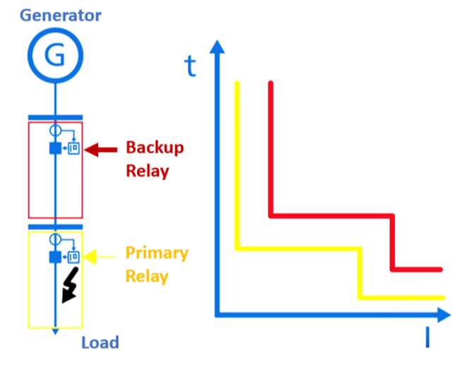
Figure 1: Inverse-time over-current curve [1]

Traditional over-current relays mentioned above rely on the specific assumptions that may cause operation failures: 1) the current under normal conditions is always smaller than the short-circuit one and 2) faults cause higher short-circuit current if located closer to the relays. Therefore, there has been a substantial literature body of literature exploring advanced operating strategies for over-current relays. Most studies of improving the performance of the over-current relays focus on the aspects of coordination [2] [3], fault detection [4] and fault section estimation [5]. Among various possible methods, machine learning is popular for advanced over-current relays. Neural networks [6] [7] are applied to determine the coefficients of the inverse-time over-current curve. Other research work based on support vector machine [8] [9] directly determined the operation of the relays.

Except for over-current relays, there are other communication-free relays including directional relays and distance relays equipped in distribution systems. Overall strategy design of protective relays share the same basic idea: relays separate the state space into multiple regions to determine whether to operate and how to cooperate with others.

I-B Reinforcement Learning Applied in Power System

As a main brunch of machine learning methods, reinforcement learning offers a panel of methods that allow controllers to learn a goal-driven control law from interactions with a real system or a simulated model. During the process of reinforcement learning, agents observe the system states, take actions determined by the policy and update the policy according the feed-back rewards. In such way, they process the accumulated experience and progressively learn a control law.

As reviewed in [11], many researchers have proposed reinforcement learning based control methods over various power system operating states and across different time scales. For electricity market simulation, several market decision strategies [12] [13] have been proposed based on off-line Q-learning. Other Q-learning based methods have been applied to voltage control [14], automatic generation control [15], demand control [16] and etc. There are also several innovative methods proposed to solve transient instability problems, including transient angle instability [17] and oscillatory angle stability [18].

However, little effort has been made for the reinforcement learning based protective strategy, one of the most important control problems in power systems. The only work [19] is about using Q-learning to determine the protection strategy of all communication-based agents. The prerequisite of global communication leaves this method impractical.

I-C Contribution of This Paper

Since reinforcement learning has been considered in a variety of power system control and decision problems, it confirms the potential of reinforcement learning in power systems. In this paper, we propose a reinforcement learning based protection strategy for the relays in distribution systems. To simplify the problem, the distribution system in this paper is assume to have a radial topology, which is consistent with most of real situations. With such assumption, relays are sequentially trained to learn how to distinguish faults and normal conditions and how to cooperate with others, only based on their local measurements.

This proposed method has the following two major advantages: 1) such communication-free method solves the impractical problem existing in the previous work; and 2) according to the experiment results, it has higher reliability and operation speed when compared with traditional over-current relays.

The rest of this paper is organized as follows. Section II introduces the simulation system, the way how to model the relays, Q-learning algorithm and training procedure. Section III shows the high accuracy and operation speed of the proposed method and provides a clear interpretation of the learned policy. Conclusion and future works are given in the Section IV.

II Problem Formulation

II-A Protective Relays

In order to precisely characterize the operation of protective relays, we first explain what (ideal) relays are supposed to do using a concrete setting given in Fig. 2. This is a single-source radial system that mimics the common application instances of over-current relay coordination and this is used as a test case in the standard literature on protective relays [c1, c2]. There are three relays respectively protecting three segments of the distribution line. Each relay is located to the right of a bus, clearing any fault that happens between their bus and the next bus to the right.

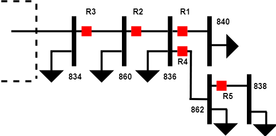
Figure 2: Protective Relays in Radial Network

The desired operation of relays are as follows. Each relay needs to protect its own region, which is between its own bus and the first down-stream bus. For improved reliability, relays that are not at the end of the line also needs to provide backup for its first downstream neighbor: when its neighbor fails to operate for any reason, it needs to trip the line and clears the fault. For example, in Fig. 2, if a fault occurs between bus 4 and 5, relay 1 is the main relay protecting this segment and it should trip the line immediately. If relay 1 fails to work, relay 2, which provides backup for relay 1, needs to trip the line instead. The time delay between detecting and clearing a fault should be as short as possible for primary relays, while backup relays should react slower to ensure that they are only triggered when the corresponding main relay is not working.

According to the above description, the desired operation of a network of protective relays can be formalized as follows. Suppose there are $n$ relays. Denote the control action of $i$th relay as $A_{i}$ and the index of its downstream neighbor as $n_{i}$. For $A_{i}$, 1 means to trip while 0 means to hold. Let $X_{p_{i}}$ and $X_{b_{i}}$ respectively be the primary and backup protection region of relay $i$. Suppose $X_{f}$ is the location of the fault, then the ideal control action $A_{i}$ of relay $i$ can be characterized as

$$A_{i}=\mathbbm{1}((X_{f}{\in}X_{P_{i}})\cup((X_{f}{\in}X_{b_{i}})\cap(A_{n_{i}}=0)))$$

where $\mathbbm{1}(\cdot)$ is an indicator function.

However, each relay in practice only knows the local measurements including voltage, current and power. Further, since relays are not aware of downstream neighbors’ actions, to prevent their conflicts, a basic idea is using time delays to achieve the correct coordination. Let $s_{i}(t)$ be the local states of $i_{th}$ relay at time $t$. Designing a protection strategy is to find a function $T_{i}$ such that:

$$a_{i}(t)=T_{i}(s_{i}(t)|\theta_{i})\ for\ i=1,...,n$$

where $n$ is the number of relays, $\theta_{i}$ is the parameters of $T_{i}$, $a_{i}(t)$ is the time delay for tripping. For convenience, define $a_{i}(t)$: when it is finite positive, it indicates the time delay for tripping; when it is positive infinite, it means to hold. An optimal protection strategy is to find $T_{i}$ that minimizes $a_{i}(t)$ and guarantees

$$0\leq{a_{i}(t)}<\infty\ if\ X_{f}{\in}X_{P_{i}}$$

and

$$a_{i}(t)-a_{n_{i}}(t)>\xi\ if\ X_{f}{\in}X_{b_{i}}$$

where $\xi$ is a security margin.

II-B Protective Relay Problem as an MDP

Markov decision processes (MDP) is a canonical formalism for stochastic control problems. The goal is to solve sequential decision making (control) problems in stochastic environments where the control actions can influence the evolution of the state of the system. In this section, we formulate the optimal relay protection strategy as the solution of an MDP.

II-B1 MDP Model

We first give a brief summary of the MDP theory. An MDP is a tuple $(\mathcal{S},\mathcal{A},R,P,\gamma)$ where $\mathcal{S}$ is the state space, $\mathcal{A}$ is the action space. $P=(P(\cdot|s,a),(s,a)\in\mathcal{S}\times\mathcal{A})$ are the state tranistion probabilities. $P(s^{\prime}|s,a)$ specifies the probability of transition to $s^{\prime}$ upon taking action $a$ in state $s$. $R:\mathcal{S}\times\mathcal{A}\rightarrow\mathbb{R}$ is the reward function, and $\gamma\in[0,1)$ is the discount factor.

A policy $\pi:\mathcal{S}\rightarrow\mathcal{A}$ specifies the control action to take in each possible state. The performance of a policy is measured using the metric of value of a policy, $V_{\pi}$, defined as

$$V_{\pi}(s)=\mathbb{E}\left[\sum^{\infty}_{t=0}\gamma^{t}R(s_{t},a_{t})|s_{0}=s\right],~{}\text{where,}$$

$$a_{t}=\pi(s_{t}),s_{t+1}\sim P(\cdot|s_{t},a_{t}).$$

The optimal value function $V^{*}$ is defined as

$$V^{*}(s)=\max_{\pi}~{}V_{\pi}(s)$$

Given $V^{*}$, the optimal policy $\pi^{*}$ can be calculated using the Bellman equation as

$$\pi^{*}(s)=\arg\max_{a\in\mathcal{A}}~{}(R(s,a)+\gamma\sum_{s^{\prime}\in\mathcal{S}}P(s^{\prime}|s,a)V^{*}(s^{\prime}))$$

Similar to the value function, Q-value function of a policy $\pi$, $Q_{\pi}$, is defined as

$$Q_{\pi}(s,a)=\mathbb{E}\left[\sum^{\infty}_{t=0}\gamma^{t}R(s_{t},a_{t})|s_{0}=s,a_{0}=a\right]$$

Optimal Q-value function $Q^{*}$ is also defined similarly, $Q^{*}(s,a)=\max_{\pi}Q_{\pi}(s,a)$. Optimal Q-value function will help us to compute the optimal policy directly without using the Bellman equation, as

$$\pi^{*}(s)=\arg\max_{a\in\mathcal{A}}~{}Q^{*}(s,a)$$

II-B2 Protective Relay as MDP

We model the protective relays as collection of MDP agents. Each relay can only observe its local measurement of voltage and current. Each relay also knows the status of the local current breaker circuits, i.e., if it is open or close. Since relays don’t observe the measurements at other relays, an implicit coordination mechanism is also needed in each relay. This is achieved by including a local counter that ensure the necessary time delay in its operation as backup relay. These variables constitute the state $s_{i}(t)$ of each relay $i$ at time $t$. Table I summarizes this state space representation. Note that the state representation include the past $m$ measurements of voltage and current.

State Variable	Description
Voltage	Voltage measurements of past $m$ timesteps
Current	Current measurements of past $m$ timesteps
Status	Current breaker state: open or close
Counter	Current value of the time counter

TABLE I: Relay State Space

To define the action space clearly, we first specify the possible action each relay can take. When a relay detects a fault it will decide to trip. However, to facilitate the coordination between the network of relays, rather than tripping instantaneously, it will trigger a counter with a time countdown, indicating the relay will trip after certain time steps. If the fault is cleared by another relay during the countdown, the relay will reset the counter to prevent mis-operation. Table II summarizes the action space of each relay.

Action	Description
Countdown	Continue the counter
Set	Set counter to value 1 - 9
Reset	Stop activated counter

TABLE II: Relay Action Space

The reward given to each relay is determined by its current action and fault status. A positive reward occurs if, i) it remains closed during normal conditions, ii) it correctly operates after a fault in its assigned region or in its first downstream region when the corresponding main relay failed. A negative reward is caused by, i) mis-operation under normal conditions; 2) tripping after a fault outside its assigned region. The magnitude of the rewards are designed in such a way to facilitate the learning, implicitly signifying relative importance of false positives and true negatives. The reward function for each relay is shown in Table III.

Condition	Trip	Hold
Normal	-150	+3
After fault in main region	+120	-3 for each post-fault step
After fault as backup	+100	-2 for each post-fault step
After fault outside assigned region	-150	+5

TABLE III: Rewards

Given an MDP formulation, the optimal value/Q-value function ($V^{*}/Q^{*}$) or the optimal control policy ($\pi^{*}$) can be computed using dynamic programming methods like value iteration or policy iteration [L]. However, these dynamic programming method requires the knowledge of the full model of the system, namely, the transition kernel $P$ and reward function $R$. In most real world applications, the stochastic system model is either unknown or extremely difficult to model. In the protective relay problem, the probability transition kernel represents all the possible stochastic variations in voltage and current in the distribution network, due a large number of scenarios like weather (and the resulting shift in demand/supply) and renewable energy generation. In these scenarios, the optimal policy has to be learned from through the repeated interactions with environment and from the state/reward observations.

II-C Reinforcement Learning

Reinforcement learning (RL) is a method for computing the optimal policy for an MDP when the model is unknown. RL achieves this without explicitly constructing an empirical model. Instead, it directly learns the optimal Q-value function or optimal policy from the sequential observation of states and rewards.

Q-learning is one of the most popular RL algorithm which learn the optimal $Q^{*}$ from the sequence of observations $\left(s_{t},a_{t},R_{t},s_{t+1}\right)$. Q-learning algorithm is implemented as follows. At each time step $t$, the RL agent updates the Q-function $Q_{t}$ as

$$Q_{t+1}(s_{t},a_{t}) =(1-\alpha_{t})Q_{t}(s_{t},a_{t})$$

$$\hskip 28.45274pt+\alpha_{t}(R_{t}+\gamma\max_{b}Q_{t}(s_{t+1},b))$$

where $\alpha_{t}$ is the step size (learning rate). It is known that if each-state action pairs is sampled infinitely often and under some suitable conditions on the step size, $Q_{t}$ will converge to the optimal Q-function $Q^{*}$[sutton2018reinforcement].

Using a standard tabular Q-learning algorithm as described above is infeasible in problems with continuous state/action space. To address this problem, Q-function is typically approximated using a deep neural network, i.e., $Q(s,a)\approx Q_{w}(s,a)$ where $w$ is the parameter of the neural network. Deep neural networks have achieved tremendous success in both supervised learning (image recognition, speech processing) and reinforcement learning (AlphaGo games) tasks. They can approximate arbitrary functions without explicitly designing the features like in classical approximation techniques. The parameter of the neural network can be updated using a (stochastic) gradient descent with step size $\alpha$ as

$$w =w+\alpha\nabla Q_{w}(s_{t},a_{t})$$

$$\hskip 28.45274pt(R_{t}+\gamma\max_{b}Q_{w}(s_{t+1},b)-Q_{w}(s_{t},a_{t}))$$ (1)

Unlike supervised learning algorithm, the data samples $(s_{t},a_{t},R_{t},s_{t+1})$ obtained by an RL algorithm is correlated in time due to the underlying system dynamics. This often leads to a very slow convergence or non-convergence of the gradient descent algorithms like (II-C). The idea of experience replay is to break this temporal correlation by randomly sampling some data points from a buffer of previously observed (experienced) data points to perform the gradient step in (II-C) [mnih2015human]. New observation are then added to the replay buffer and the process is repeated.

In the gradient descent equation (II-C), the target $R_{t}+\gamma\max_{b}Q_{w}(s_{t+1},b)$ depends on the neural network parameter $w$, unlike the targets used for supervised learning which are fixed before learning begins. This often leads to poor convergence in RL algorithms. To addresses this issue, deep RL algorithms maintain a separate neural network for the target. The target network is kept fixed for multiple steps. The update equation with target network is given below.

$$w =w+\alpha\nabla Q_{w}(s_{t},a_{t})$$

$$\hskip 28.45274pt(R_{t}+\gamma\max_{b}Q_{w^{-}}(s_{t+1},b)-Q_{w}(s_{t},a_{t}))$$

$$w^{-}=w\quad\text{after every $N$ steps.}$$

The combination of neural networks, experience replay and target network forms the core of the DQN algorithm [mnih2015human].

In the following, we use the DQN algorithm for training each relay.

III Experiment Design

III-A Environment Implementation

The testbed shown in Fig. 2 is implemented using Power System Simulator for Engineering (PSS/E) by Siemens, a commercial power system simulation software. The simulation process is controlled by Python using the official PSSPY interface library and the dynamic simulation module. The environment is wrapped according to the OpenAI Gym[22] format that provides APIs for agents to start, step through and end an episode.

In this context, an episode is defined as a short simulation segment that contains a fault. In the beginning of each episode, the operating condition (e.g. generator output, load size) is randomized to mimic the load deviation of distribution systems. During an episode, a fault is added to the system at a random time-step. The fault is set to have random fault impedance within a range determined according to the proposed model in [23] and occurs at a random location. Each step, the environment receives actions from the agents, simulates for another step according to the actions and returns the corresponding state variables and reward to each agent. To create cases that require the backup mechanic, the environment has a probability to ignore a trip action from an agent, which corresponds to the case when the breaker fails as a relay tries to trip the line. In this case, the first upstream relay needs to trip the line instead.

In practice, the load level of distribution systems varies a lot with the time of day. To simulate this, the system is assigned a random trend factor from 70% to 130% in the beginning of each episode. On top of that, each of the 5 loads in the system have their own load multiplier between 80% and 120% of the system-wide trend factor. The capacity of each load is determined by multiplying the base case capacity and the local multiplier. A powerflow solution is then calculated using the random load profile as the initial condition for the dynamic simulation.

III-B Training Strategy

III-B1 Single Relay System

Using th environment described above, the relays can be trained to protect the system. We first present the process of training relay 1, which is the simplest case as it does not need to consider coordination with other relays. The expected operation of relay 1 is exactly the same as in a single-relay system: it needs to trip for any fault in its primary region, and remain closed for other faults. There is no coordination with other relays, so the operation of relay 1 is independent. The policy of relay 1 is trained by running many random episodes and updating the DQN such that it gives the action that maximizes the expected total reward. During the training of relay 1, the other relays are deactivated since their operation would not have any impact on the optimal policy of relay 1. The complete training process of relay 1 is shown in Algorithm 1.

Algorithm 1 Training Process of Single Relay System

  Initialize DQN weights

  Initialize replay buffer

  repeat

     Initialize PSS/E simulation with random parameters

     repeat

        Read observations for relay 1 $S$ from PSS/E

        Choose action A[i] using $\epsilon-greedy$

        Send action $A$ to PSS/E

        Receive reward $R$ and next state $S^{\prime}$

        Store $(S,A,R,S^{\prime})$ to replay buffer

        if Buffer size $\geq$ N then

           Randomly sample a batch of size N from replays

           Update DQN weights using the sampled batch

        end if

     until Current episode terminated

  until Iteration limit reached or DQN converged

III-B2 Multi-Relay System

When there are multiple relays operation in the same system, the coordination between relays becomes a Multi-Agent Reinforcement Learning (MARL) problem. If a relay needs to provide backup for another relay, its policy needs to adapt to the policy of its downstream neighbor. When training the relays under this context, the assumption required for Q-Learning to converge is violated since the policies of all agents are constantly changing, making the environment non-static from the perspective of every agent. Moreover, since communication between agents is not practical, each agent can only observe the environment from their own location. The formulation that involves these two constraints is known as Decentralized Partially Observable Markov Decision Process (Dec-POMDP)[24]. There are existing literatures[25][26] addressing this kind of problems, but the performance of most algorithms are unstable and the convergence is hardly guaranteed. However, this problem can be greatly simplified by taking advantage of the environment’s special structure, to the extent that even a simple single-agent DQN algorithm can perform well.

To further explain why the environment structure can help on simplifying the problem, we start from the very end of the radial network in Fig. 2. The relay protecting the last segment is relay 1, which has no downstream neighbors and can be trained using the single-agent training method described in the previous section. After the training of relay 1 is finished, it will react to the system dynamics using its policy. Since relay 1 only needs to clear local faults (i.e. faults between bus 4 - 5) and ignores disturbances at any other location, its policy does not need to change after training relay 2 and 3. This enables us to train relay 2 with relay 1 in commission. Since the policy of relay 1 remains fixed when training relay 2, the environment from the perspective of relay is no longer changing. Similarly, after the training of relay 2 is complete, relay 3 can be trained with the policy of relay 1 and 2 remain fixed. The sequential-training approach allows us to get around the assumption violation in typical MARL problems and use the many nice features of single-agent algorithms to train the relays. The training process for each relay in a multi-relay system is shown in Algorithm 2.

Algorithm 2 Training Process for Systems with N relays

  Initialize DQN weights

  Initialize replay buffer

  for Relay number i = 1 to N do

     repeat

        Initialize PSS/E simulation with random parameters

        repeat

           Read observations for all relays $S$ from PSS/E

           Initialize Action vector $A$ = $zeros(N)$

           Choose action A[i] using $\epsilon-greedy$

           for Relay number j = 1 to i do

              Set action A[j] = $\operatorname*{arg\,max}_{a}Q(S[i],a)$

           end for

           for Relay number k = i+j to N do

              Set action A[k] = 0

           end for

           Send action vector $A$ to PSS/E

           Receive reward $R$ and next state $S^{\prime}$

           Store $(S,A,R,S^{\prime})$ to replay buffer

           if Replay buffer size $\geq$ M then

              Randomly sample a batch of size M from buffer

              Update DQN weights using the sampled batch

           end if

        until Current episode terminated

     until Iteration limit reached or DQN converged

  end for

III-C Agent Implementation

The relays are implemented using the open-source library Keras-RL[27]. All 3 agents use the same model shown in Table. IV. Since the Python interface of PSS/E(i.e. the Environment) and TensorFlow(i.e. the Agents) is inherently incompatible, they must run on two separate processes simultaneously. The environment is wrapped as a TCP/IP server that accepts connections through a pre-allocated port and keeps running in the background. While agents communicate with the server using the same port via $localhost$. Also, to accommodate the TCP/IP requirement, a dedicated encoder/decoder pair is also written to pack the data as byte strings before transmitting through the port.

TABLE IV: Agent DQN Model

Property	Description
Hidden Layers	2
Layer Size	128/64
Activation	ReLU/ReLU/Linear
Optimizer	Adam
Loss	MSE

IV Results and Discussion

IV-A Agent Training

The 3 relays are implemented and trained using the strategy discussed in Sec. III B. Relay 1 is trained using the single-relay approach described in Algorithm 1, in which the other relays are disabled during simulation. The learning curves of relay 1 is plotted by running multiple trials of the training process and recording the convergence trajectory. Fig. 3 shows the convergence of episodic reward and the convergence of incorrect operation during training. It can be seen from the plots that the policy of relay 1 converges stably, as the number of incorrect operation gradually vanishes along the training process.

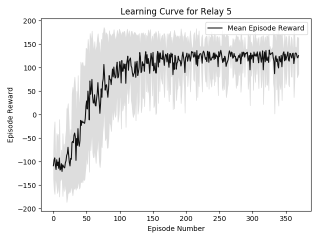
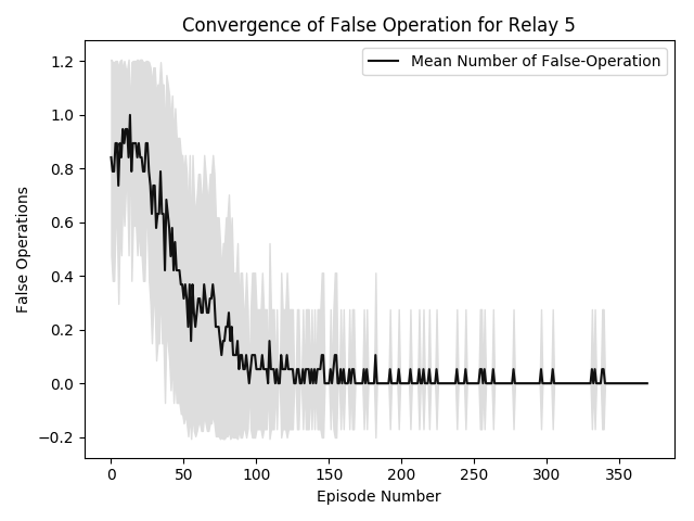
Figure 3: Convergence Plots of Single Relay

Relay 2 and 3 are trained using the multi-relay approach in Algorithm 2, where the trained policies of downstream relays obtained previously are used in training. Since the operation of relays that need to coordinate with others is more complex than the single relay case, a longer training time is needed before the policy stabilizes. The convergence plot of backup relays are shown in Fig. 4.

IV-B Experiment Result

The trained agents are put in to the same stochastic environment to evaluate their performance. The scenarios are divided into 3 categories: Operation for the main region, backup for the downstream neighbor and faults at other locations. The performance on each category is tested on 5000 random episodes. There are two kinds of wrong operations: false-negative and false-positive. False-positive means that a relay trips the line when there is no fault, the location of fault is outside of the relay’s assigned region or trips before the primary relay. False-negative means that a relay never operated in the entire episode when the fault is inside the relay’s assigned region or the immediate downstream neighbor is deactivated. In each episode, the number of failed or mis-operation is the sum of such operations from all 3 relays. Results of the test are documented in Table. V.

TABLE V: Categorized Test Result on Random Environment

Scenario	Expected Operation	False positive	False negative	Success Rate
Local Fault	Trip	N/A	13	99.74%
Backup	Trip	N/A	0	100%
Remote Fault	Hold	4	N/A	99.92%
No Fault	Hold	0	N/A	100%

The agents also demonstrate very fast tripping speed during the test. The simulation step length is 1/10 of a cycle, which equals 600 steps per second. In the end of each step, the recorded voltage and power are fed to the agents as observations. The operation speeds of the agents are measured in steps, and is shown in Table VI. The operation speeds of the 3 agents are roughly the same. It can be seen that all relays react to the fault very quickly.

TABLE VI: Operation Speed of Agents

Type	Average Operation Time in Step	Average Operation Time in Second
Local Fault	3	0.005
Backup	5	0.00833

IV-C Comparison With Traditional Strategy

Traditional over-current relays operate based on a set current threshold, which is determined under the assumption that normal current is always ignorable compared to fault current. The threshold is also computed based on a fixed operating condition (i.e. substation feeder capacity and load profile). However, in distribution systems, where over-current relays are mostly used, the load profile greatly varies with the time of day. Moreover, with the increasing penetration of renewable and distributed generation, the load variation is expected to be even more diverged. Under realistic large load variation, the initial assumption of over-current relays can be violated, since the fault current cannot be assumed to be much larger than normal current across different scenarios. In fact, when the system is lightly loaded, the fault current with a relatively large fault impedance can even be smaller than the normal operating current when the system is heavily loaded.

To demonstrate this, the distribution of measured current at bus 4 is plotted in Fig. 3. This distribution is obtained by running 500 random episodes, in which the fault is placed between bus 4 and bus 5. The current magnitude before and after the fault is sampled and plotted as a histogram. A Probability Density Function (PDF) is created by fitting the distribution recorded in the histogram. It is clearly shown in Fig. 3 that the range of pre-fault and post-fault current is overlapping with each other. Traditional relays use a fixed threshold (Pickup Current) to detect fault conditions, which means if the current measurement is greater than a pre-set value, the tripping mechanism is triggered. The threshold is reflected as a vertical line in Fig. 3. If the current measurement falls to the right of the line (i.e. current greater than pickup current), the relay is set to trip the line. Using the distribution in Fig. 3, the total number of incorrect operations can be minimized by setting the threshold to the point of intersection of the red and green curve. The optimal threshold is shown in Fig.3 as the blue line. The probability of false-positive and false-negative operations associated with the optimal threshold is calculated using the data sampled in the random tests and is shown in Table VII.

TABLE VII: Success Rate of Traditional Overcurrent Relay

Scenario	Expected Operation	Success Rate
Local Fault	Trip	92.3%
No Fault	Hold	98.3%

It can be seen that the RL based relay far out-performs the optimal traditional setting in both normal and faulty scenario. Since Relay 1 does not need to coordinate with other relays, its operation is the simpler compared to that of relay 2 and 3. With the increased complexity of backup coordination taken into account, the performance margin of RL based relay is expected to be even larger compared to traditional over-current relays.

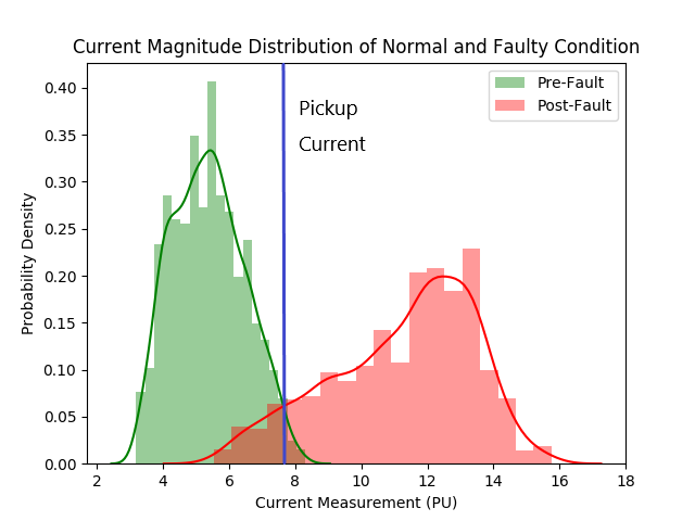
Figure 4: Distribution of Current Magnitude Measured at Bus 4

IV-D Policy Interpretation

Intuitively, the RL agents takes the advantage of making decisions based on not only the current observation, but also with the historical values several steps before. The observations stored in the FIFO buffer form a trajectory, which can be more indicative than using a single step snapshot. The trajectories formed under different scenarios (i.e. local fault, normal operation, remote fault) can be accurately classified by the agent. Fig. 4 shows the recorded observation trajectory plotted as current versus voltage. The red trajectories are taken when relay 1 trips the line for a local fault between bus 4 and 5, while the green trajectories are taken before the fault occurs during the same episode. It can be clearly seen that the trajectory strays away from the normal trail when a fault happens, which results in a voltage decrease and current increase. Such sudden change in the observation is captured by the agents as a measure to interpreted the current system condition.

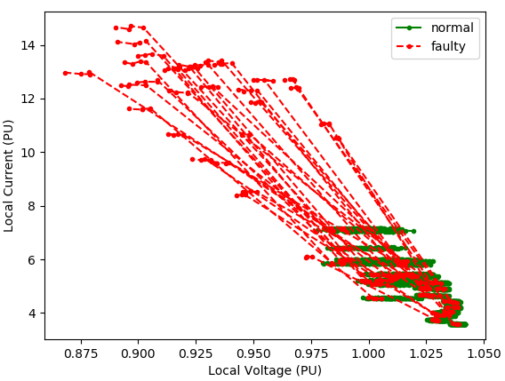
Figure 5: Observation Trajectories During Normal and Fault Condition

V Conclusion and Future Works

V-A Advantages of RL Based Relays

We have proposed a RL based relaying strategy, where the relays are modeled as DQN agents and trained in a stochastic simulation environment. The RL based relays demonstrated various advantages over traditional over-current settings. Firstly, after training in the simulation environment, the agents can reliably identify the system condition and fault location under large load variation and different fault scenarios. With a special sequential training strategy, the agents can also coordinate with their downstream neighbor to accomplish backup operation. Secondly, the reaction time of the agents is very short, typically within half of a cycle. This allows the breaker to clear the fault quickly and prevent damages on equipments. Thirdly, in contrast to many proposed new relay control strategy in published literatures, the RL based relays do not require any communication with the data center or other relays, which makes implementation simpler and cheaper.

V-B Practical Considerations

Apart from the performance advantage of RL based relays, they are also easy to train and deploy to real distribution systems. Their biggest advantage lies in the ability to work without communication. In practice, many distribution systems are not designed to carry communication lines between towers or power line transmission devices, which makes communication based designs relatively hard to implement and cost ineffective. Our purposed RL based relay can achieve very good performance while still being communication-free. The core engine of a RL based relay (i.e. the trained neural network) is also easily programmable as the network size is very small. It can be implemented using either a general-purpose micro-controller or specially designed AI chip.

V-C Challenges and Future Directions

On top of this paper, there is great potential in exploring the possible applications of rapidly developing reinforcement learning strategies in the field of power system protection. Based on this paper, future works may include RL based relay design in systems with distributed generation and/or different network topologies. Enabling communication between agents or training use a multi-agent approach could have better performance for more complex systems. Furthermore, RL approaches could also be used in other parts of power system protection, such as precise fault locating, device protection or automatic re-closing.

References

- [1] OMICRON Energy, “How does overcurrent protection work?”, YouTube, 2017, [Online]. Available: https://www.youtube.com/watch?v=bQ6fZrrP0H4. [Accessed: 06-Mar-2019].
- [2] W. El-Khattam and T. S. Sidhu, “Restoration of directional overcurrent relay coordination in distributed generation systems utilizing fault current limiter”, IEEE Transactions on Power Delivery, 2008, vol. 23, no. 2, pp. 576–585
- [3] H. Zhan, C. Wang, Y. Wang, X. Yang, X. Zhang, C. Wu, and Y. Chen, “Relay protection coordination integrated optimal placement and sizing of distributed generation sources in distribution networks”, IEEE Transactions on Smart Grid, 2016, vol. 7, no. 1, pp. 55–65
- [4] P. Dash, S. Samantaray, and G. Panda, “Fault classification and section identification of an advanced series-compensated transmission line using support vector machine”, IEEE transactions on power delivery, 2007, vol. 22, no. 1, pp. 67–73
- [5] H.-T. Yang, W.-Y. Chang, and C.-L. Huang, ”A new neural networks approach to on-line fault section estimation using information of protective relays and circuit breakers”, IEEE Transactions on Power delivery, 1994, vol. 9, no. 1, pp. 220–230
- [6] P. Mahat, Z. Chen, B. Bak-Jensen and C.L. Bak, ”A Simple Adaptive Overcurrent Protection of Distribution Systems With Distributed Generation”, IEEE Transactions on Smart Grid, 2011, vol.2, no.3, pp 428-437
- [7] H. A. Abyane, K. Faez and H. K. Karegar, ”A new method for overcurrent relay (O/C) using neural network and fuzzy logic”, TENCON ’97 Brisbane - Australia. Proceedings of IEEE TENCON ’97. IEEE Region 10 Annual Conference: Speech and Image Technologies for Computing and Telecommunications (Cat. No.97CH36162), Brisbane, Queensland, Australia, 1997, pp. 407-410 vol.1
- [8] D. N. Vishwakarma and Z. Moravej, ”ANN based directional overcurrent relay”, 2001 IEEE/PES Transmission and Distribution Conference and Exposition. Developing New Perspectives (Cat. No.01CH37294), 2001, Atlanta, GA, USA, pp. 59-64 vol.1
- [9] Y. Zhang, M. D. Ilic and O. Tonguz, ”Application of Support Vector Machine Classification to Enhanced Protection Relay Logic in Electric Power Grids”, 2007 Large Engineering Systems Conference on Power Engineering, 2007, Montreal, Que., pp. 31-38
- [10] X. Zheng, X. Geng, L. Xie, D. Duan, L. Yang and S. Cui, ”A SVM-based setting of protection relays in distribution systems”, 2018 IEEE Texas Power and Energy Conference (TPEC), 2018, College Station, TX, pp. 1-6.
- [11] M. Glavic, R. Fonteneau and D. Ernst, ”Reinforcement Learning for Electric Power System Decision and Control: Past Considerations and Perspectives”, IFAC-PapersOnLine, 2017, vol. 50, no. 1, pp. 6918-6927
- [12] B. Kim, Y. Zhang, M. van der Schaar and J. Lee, ”Dynamic Pricing and Energy Consumption Scheduling With Reinforcement Learning”, IEEE Transactions on Smart Grid, 2016, vol. 7, no. 5, pp. 2187-2198
- [13] R. Lincoln, S. Galloway, B. Stephen and G. Burt, ”Comparing Policy Gradient and Value Function Based Reinforcement Learning Methods in Simulated Electrical Power Trade”, IEEE Transactions on Power Systems, 2012, vol. 27, no. 1, pp. 373-380
- [14] Y. Xu, W. Zhang, W. Liu and F. Ferrese, ”Multiagent-Based Reinforcement Learning for Optimal Reactive Power Dispatch”, IEEE Transactions on Systems, Man, and Cybernetics, Part C (Applications and Reviews), 2012, vol. 42, no. 6, pp. 1742-1751
- [15] T. Yu, B. Zhou, K. W. Chan, L. Chen and B. Yang, ”Stochastic Optimal Relaxed Automatic Generation Control in Non-Markov Environment Based on Multi-StepLearning”, IEEE Transactions on Power Systems, 2011, vol. 26, no. 3, pp. 1272-1282
- [16] F. Ruelens, B. J. Claessens, S. Vandael, B. De Schutter, R. Babuška and R. Belmans, ”Residential Demand Response of Thermostatically Controlled Loads Using Batch Reinforcement Learning”, IEEE Transactions on Smart Grid, 2017, vol. 8, no. 5, pp. 2149-2159
- [17] M. Glavic, ”Design of a resistive brake controller for power system stability enhancement using reinforcement learning”, IEEE Transactions on Control Systems Technology, 2005, vol. 13, no. 5, pp. 743-751
- [18] T. Ademoye and A. Feliachi, ”Reinforcement learning tuned decentralized synergetic control of power systems”,Electric Power Systems Research, 2012, vol. 86, pp. 34-40
- [19] H. C. Kiliçkiran, B. Kekezoglu and G. Nikolaos Paterakis, ”Reinforcement Learning for Optimal Protection Coordination”, 2018 International Conference on Smart Energy Systems and Technologies (SEST), Sevilla, 2018, pp. 1-6
- [20] V. Minh et al., ”Human-level control through deep reinforcement learning”, Nature, 2015, 518.7540:529
- [21] M. Abadi et al., ”TensorFlow: Large-scale machine learning on heterogeneous systems”, software available from tensorflow.org
- [22] G. Brockman, V. Cheung, L. Pettersson, J. Schneider, J. Schulman, J. Tang and W. Zaremba, OpenAI Gym, 2016, arXiv:1606.01540
- [23] D.A.S. José and S. Elmer, ”Typical expected values of the fault resistance in power systems”, 2010 IEEE/PES Transmission and Distribution Conference and Exposition: Latin America, T and D-LA 2010. 602 - 609. 10.1109/TDC-LA.2010.5762944.
- [24] S. Kapoor, ”Multi-Agent Reinforcement Learning: A Report on Challenges and Approaches”, Computing Research Repository, arXiv, 2018, arXiv:1807.09427
- [25] R. Lowe, Y. Wu, A. Tamar, J. Harb, P. Abbeel and I. Mordatch, ”Multi-Agent Actor-Critic for Mixed Cooperative-Competitive Environments”, Advances in Neural Information Processing Systems, 2017, pp. 6379-6390
- [26] L. Kraemer and B. Banerjee, ”Multi-Agent Reinforcement Learning as a Rehearsal for Decentralized Planning”, Neuralcomputing, 2016, 190:82-94
- [27] M. Plappert, keras-rl, GitHub Repository, 2016, https://github.com/keras-rl/keras-rl