Lead-lag Relationships in Foreign Exchange Markets

Abstract

Lead-lag relationships among assets represent a useful tool for analyzing high frequency financial data. However, research on these relationships predominantly focuses on correlation analyses for the dynamics of stock prices, spots and futures on market indexes, whereas foreign exchange data have been less explored. To provide a valuable insight on the nature of the lead-lag relationships in foreign exchange markets here we perform a detailed study for the one-minute log returns on exchange rates through three different approaches: i) lagged correlations, ii) lagged partial correlations and iii) Granger causality. In all studies, we find that even though for most pairs of exchange rates lagged effects are absent, there are many pairs which pass statistical significance tests. Out of the statistically significant relationships, we construct directed networks and investigate the influence of individual exchange rates through the PageRank algorithm. The algorithm, in general, ranks stock market indexes quoted in their respective currencies, as most influential. In contrast to the claims of the efficient market hypothesis, these findings suggest that all market information does not spread instantaneously.

1 Introduction

Financial systems consist of many units influencing each other through interactions of different nature and scale, thereby exhibiting rather complex dynamics. The time series of the system observables, which capture these dynamics, are functions with pronounced random components. Hence, one requires convenient statistical tools to infer both the behavior of individual units and the overall performance of the financial system. In this aspect, a lot of effort has been put into developing tools for studying the pairwise relationships between assets as they provide direct estimate for the intensity of the mutual interactions. Besides this, the pairwise relationships also have particular practical relevance in construction of optimal portfolios and efficient asset allocations. As a result, various statistical approaches have been applied to plethora of financial markets, among which, equity prices at stock markets [1, 2], currencies at foreign exchanges [3, 4] and even market indexes [5].

The majority of these studies mainly focus on relationships based on simultaneous observations of the logarithmic returns of the examined assets. The results obtained from such studies are able to explain the mutual interactions only when the time needed for spreading of the news across the financial market is negligible in comparison to the period of calculation of log returns. The relevance of the results obtained in such situations is backed by the efficient market hypothesis. The hypothesis states that the current price of any asset traded in the market incorporates all relevant information and no prediction regarding the future evolution would be profitable without taking additional risks [6]. Numerous studies confirm that in practice this usually holds when one considers log returns on daily or longer time scale. When shorter time scales are considered, such as one-minute log returns, one might expect significant delay effects. To address this issue, one usually resorts to the usage of lagged approaches. These approaches give estimates for the relationship between the observations of the two quantities of interest which are apart from each other for certain period  [7, 8]. The variable whose values are delayed is called the lagger, whereas the other one is the leader.

Research on these lead-lag relationships predominantly focuses on correlation analyses of dynamics of stock prices or market indexes [9, 10, 11]. To the best of our knowledge, the examination of the lead-lag relationships in a foreign exchange market remains largely unexplored. To bridge this gap, here we study the relationships between one-minute log returns on exchange rates with a lag of one minute. We focus on returns lagged for one minute due to three reasons. First, even though past research suggests that the lead-lag relationships can be felt in the price of the lagger even up to 45 minutes later, as trading becomes more and more automatic, the lagging period has decreased dramatically to typical value measured in seconds [9], or even milliseconds [12]. Second, the foreign exchange is known to be a very liquid one, with most of the transactions being ordered automatically and one can not expect significant lags that span longer than one minute. This reasoning was supported by studying lagged effects with two-minute lags. In this case, we found that although such lagged relationships might appear sporadically, the pattern is not persistent as it is when one-minute lags are considered.

We consider three different approaches to estimate the lead-lag relationships: i) lagged correlations, ii) lagged partial correlations and iii) Granger causality. The lagged correlations provide a direct estimate for the intensity of linear lead-lag relationship between two exchange rates. The lagged partial correlations extend this approach by eliminating the possible serial autocorrelation of the lagger and the contemporaneous correlation of both rates under study. Finally, the Granger causality [13] statistically tests for possible causal relationship between two exchange rates by considering the predictive potential by using past returns. We find that, with few exceptions, the lagged correlations between exchange rate pairs which relate currencies do not pass tests of statistical significance, which is in accordance with the efficient market hypothesis. However, there are many statistically significant lagged correlations, particularly when one considers rates which involve stock market indexes. In these correlation coefficients, the stock market indexes, which are known to have slower dynamics than the currency exchange raters, appear as leaders. Interestingly, this is opposite to previous findings which suggest that assets with faster dynamics behave as leaders [7, 8, 14]. The partial correlation analysis further confirmed our findings. The Granger causality analysis, in addition to providing a test for the findings in the correlation analysis, revealed that the leaders in the lead-lag relationships also increase the predictive ability for the determination of future returns of the lagger. Based on these observations one could believe that the information from the leader towards the lagger does not transfer simultaneously, but it can be seen as a process that stretches for a certain period.

Out of the statistically significant pairwise correlations and causality relationships we obtained matrices, which can be regarded as directed networks that describe the effect of one asset towards another. To infer the most influential leaders, in the spirit of [15], we apply the PageRank algorithm. PageRank is a widely used procedure that has been applied in original or modified form to various domains [16, 17, 18, 19]. The resulting ranking allows us to infer the major sources of information spillover in the studied financial network.

The outline of the paper is as follows. In Section 2 we introduce the methods applied for the estimation of the lagged correlations, lagged partial correlations and causality, as well as the generation of the resulting networks. Section 3 presents the empirical results. The last section summarizes our findings and provides directions for future research.

2 Methods

2.1 Lagged correlations

The dynamics of the prices of financial assets are known to be non-stationary. Hence, one can not simply use them to examine the relationship between different assets. Nevertheless, the logarithmic return,

$$r_{n}=\log p(t_{n+1})-\log p(t_{n}),$$ (1)

where the price $p$ is assumed to be observed at discrete moments $t_{n}$, is usually assumed to be weakly stationary [20]. This property of log returns makes them more appropriate quantities for uncovering statistical relationships between assets.

Assuming that we have observations of the log returns $r_{i}$ and $r_{j}$ of two prices at the series of discrete moments $t_{n}$, the $\tau$-lagged covariance between them is given by

$$C_{i,j}(\tau)=\langle\left[r_{i}\left(t_{n}\right)-\langle r_{i}\rangle\right]\left[r_{j}\left(t_{n}+\tau\right)-\langle r_{j}\rangle\right]\rangle,$$ (2)

where the angular brackets denote averaging. We emphasize that one should keep the order of indices since in this notation the first index is the leader, while the second denotes the lagger. In general, the lagged covariances are not commutative $C_{i,j}(\tau)\neq C_{j,i}(\tau)$, in contrast to the ordinary, zero-lag covariances. Since the log return of one price might typically deviate more than that of the other one, a more appropriate quantity is the correlation coefficient

$$\rho_{i,j}(\tau)=\frac{C_{i,j}(\tau)}{\sqrt{C_{i,i}(0)C_{j,j}(0)}}=\frac{C_{i,j}(\tau)}{\sigma_{i}\sigma_{j}}.$$ (3)

In the last expression the notation is simplified by using the standard deviation $\sigma_{i}=\sqrt{C_{i,i}}$.

2.2 Lagged partial correlations

In reality, the existence of lagged correlation can be due to one exchange rate being the driving force of the other, or due to the combination of mutual contemporaneous correlation and lagged autocorrelation. In order to isolate this potential effect, we calculate the partial correlation coefficient. For three random variables $X$, $Y$, and $Z$ with respective pairwise correlations $\rho(X,Y)$, $\rho(Y,Z)$, and $\rho(X,Z)$, the partial correlation between $X$ and $Y$ with $Z$ considered known, is defined as

$$\rho(X,Y|Z)=\frac{\rho(X,Y)-\rho(X,Z)\rho(Y,Z)}{\sqrt{[1-\rho^{2}(X,Z)][1-\rho^{2}(Y,Z)]}}.$$ (4)

Therefore, when the current return of the lagger $j$ has the role of known variable, the correlation between its next value and current return on the leader $i$ is

$$\rho_{i,j}^{P}(\tau)=\frac{\rho_{i,j}(\tau)-\rho_{i,j}(0)\rho_{j,j}(\tau)}{\sqrt{[1-\rho_{i,j}^{2}(0)][1-\rho_{j,j}^{2}(\tau)]}}.$$ (5)

The last expression is useful when one has calculated already the values of the ordinary correlations and thus would immediately obtain the partial one. Another approach for calculation of the partial correlation is based on linear regression [21]. It can be described as follows. Let $Z$ be the variable whose influence has to be removed, the two other variables being $X$ and $Y$, and their best estimates by observing $Z$ being $\hat{X}_{Z}$ and $\hat{Y}_{Z}$ respectively. The respective partial correlation is then the ordinary correlation between the residuals $r_{X}=X-\hat{X}_{Z}$ and $r_{Y}=Y-\hat{Y}_{Z}$, given by

$$\rho(X,Y|Z)=\rho(X-\hat{X}_{Z},Y-\hat{Y}_{Z}).$$ (6)

This approach allows for easier calculation of the statistical significance of the estimated partial correlation, and as such has been widely applied in studies of relationships between currencies and stocks [22, 23, 24].

2.3 Lagged correlation networks

As the lagged correlations are not commutative (in contrast to the contemporaneous correlations), the resulting network is directed. In order to keep the strength of influence we create a weighted network where the direction is from the lagger towards the leader with weight that is equal to the absolute value of the lagged correlation coefficient $w_{j,i}=|\rho_{j,i}|$. We consider absolute values since the sign of the correlation coefficient denotes only the direction of change of the exchange rate. Typically, extraction of the core of financial correlation networks is performed with the Minimal Spanning Tree (MST) sub-graph procedure [2] or the Planar Maximally Filtered Graph (PMFG) [22, 25]. Because the obtained statistically validated lagged correlation networks are rather sparse, we may instead use the PageRank algorithm in order to determine the most influential leaders [15]. The PageRank algorithm was originally used to rank web pages, by assuming that pages with more incoming links from others are more important. A particular feature which favors PageRank above other ranking procedures is that it intrinsically assigns higher weights to links that originate from important nodes.

The application of PageRank first involves creating a row stochastic matrix from the weighted network with elements

$$a_{j,i}=\frac{w_{j,i}}{\sum_{k}w_{j,k}}.$$ (7)

The last matrix can be seen as a Markov chain transition matrix. In terms of Markov chain theory, the element $a_{j,i}$ corresponds to the probability of jumping from state $j$ to $i$. For such matrices arising from correlation networks, the bigger values within $j$-th row correspond to the columns $i$ associated with rates from which $j$ obtains larger impact. As such, the resulting rankings should provide information regarding the market news spreading among the the exchange rates included in the analysis. Higher ranking should correspond to exchange rates whose changes in returns will also have a higher overall impact in the overall system dynamics.

2.4 Granger causality

The potential influence of the return on certain exchange rate on future returns on other exchange rates can be assessed by applying the causality analysis in the sense of Granger [13]. WIthin this framework, cause and effect relationship between a pair of two dynamical variables exists if knowledge of past values of one of them improves the prediction of the future of the other. Granger causality is estimated as follows. Consider the linear regression of the nearest future value of some variable $x$ from its past $p$ terms

$$x_{n+1}=\sum_{k=0}^{p-1}\alpha_{k}x_{n-k}+\varepsilon_{n},$$ (8)

where $\varepsilon_{n}$ is the regression residual. The weights $\alpha_{k}$ are such that the residual variance $\sigma_{\varepsilon}^{2}$ is minimal, so the linear regression is optimal. Now, make an optimal combined regression by using $q$ past values of the variable $y$ as well

$$x_{n+1}=\sum_{k=0}^{p-1}\alpha_{k}x_{n-l}+\sum_{l=0}^{q-1}\beta_{l}y_{n-l}+\eta_{n}.$$ (9)

If some of the parameters $\beta_{l}$ are nonzero with certain statistical significance, which in turn leads to reduced variance $\sigma_{\eta}^{2}<\sigma_{\varepsilon}^{2}$, then it is said that $y$ Granger causes $x$. If $x$ also Granger causes $y$ than one has a feedback system. The regression depth $q$ (and $p$ as well) depends on the problem at hand. We consider only one past step, as it has been observed that in foreign exchange markets the serial autocorrelation quickly vanishes. Another reason for this choice is that, as it will be seen in the Data Section, due to the presence of gaps and periods of repeating identical values in the studied time series, there is a much smaller number of consecutive nonzero returns than the one required for a meaningful regression with more explanatory variables. Therefore, our Granger causality setting for the effect of exchange rate $i$ on exchange rate $j$ is described as

$$r_{j}(t_{n+1})=\alpha_{i,j}r_{j}(t_{n})+\beta_{i,j}r_{i}(t_{n})+\gamma_{i,j}+\eta_{i,j,n}.$$ (10)

In the last equation $\alpha_{i,j}$ estimates the self driving force, $\beta_{i,j}$ measures the influence of the return of exchange rate $r_{i}$, $\gamma_{i,j}$ accounts for possible nonzero mean return of the rate $r_{j}$, and $\eta_{i,j,n}$ is the noise term. When $\beta_{i,j}$ is zero, then $r_{j}$ is not caused by $r_{i}$, otherwise there is causal relationship from returns on rate $i$ to $j$.

The quality of a regression model is usually estimated in terms of the mean of the squared residuals. Concretely, let us denote with $S_{0}$ the variance of the dependent variable. Correspondingly, let $S$ be the mean of the square of the residuals obtained from regression of the kinds of Eqs. (8) or (10). The estimate of the quality of the model is then given by the coefficient of determination

$$R^{2}=1-\frac{S}{S_{0}}.$$ (11)

When one compares two regression models, nested into each other, one needs a way to compare them. Because the one with more parameters is expected to have better performance than the other, one needs to know whether it significantly outperforms the simpler peer. The respective tool for such estimates is the $F$-test. Consider a simpler regression model with $p_{1}$ parameters which result in residual sum of squares $S_{1}$, and its bigger alternative with $p_{2}$ parameters and residual sum of squares $S_{2}$ , applied on the same $N$ data items. Then, if both have the same quality in the null hypothesis, the respective $F$-test statistic

$$F=\frac{\frac{S_{1}-S_{2}}{p_{2}-p_{1}}}{\frac{S_{2}}{N-p_{2}}},$$ (12)

has $F$ distribution with $(p_{2}-p_{1},N-p_{2})$ degrees of freedom.

We note that a more general approach can be obtained with the vector autoregression model (VAR) [26]. VAR is a generalization of the previously explained procedure, where the log return $r_{j}(t_{n+1})$ is regressed with more than one, or even all other returns. Unfortunately, we cannot apply this procedure on the data under study, because many exchange rates have either zero return, or missing values at different moments, and the regression would then be meaningless.

3 Data

3.1 Data source

We use data gathered from www.histdata.com. The dataset contains highly frequent one-minute exchange rate values only on the bid quotes, which is a slight drawback since generally as price of an asset is considered the mean of the respective bid and ask values. Even though the bid is not simply a drifted version of the mean price, it can serve in the analysis as an estimate for the value from the point of view of the brokers.

We extract exchange rate data for 66 pairs among 33 assets consisting of 19 currencies, 10 indexes of major stock markets, 2 oil types, and gold and silver. The list of assets together with their abbreviations is given in Table 1.

Table 1: List of studied assets

Currencies
AUD – Australian Dollar	MXN – Mexican Peso
CAD – Canadian Dollar	NOK – Norwegian Krone
CHF – Swiss Franc	NZD – New Zealand Dollar
CZK – Czech Koruna	PLN – Polish Zloty
DKK – Danish Krone	SEK – Swedish Krona
EUR – EURO	SGD – Singapore Dollar
GBP – British Pound	TRY – Turkish Lira
HKD – Hong Kong Dollar	USD – US Dollar
HUF – Hungarian Forint	ZAR – South African Rand
JPY Japanese Yen
Indexes
AUX – ASX 200	JPX – Nikkei Index 400
ETX – EUROSTOXX 50	NSX – NASDAQ 100
FRX – CAC 40	SPX – S&P 500
GRX – DAX 30	UDX – Dollar Index
HKX – HAN SENG	UKX – FTSE 100
Commodities
BCO – Brent Crude Oil	XAG – Silver
WTI – West Texas Intermediate	XAU – Gold

3.2 Data preprocessing

In spite of the foreign exchange market being highly dynamic, the data which we study includes several cases where a rate has the same value in few consecutive minutes. This means that the respective one-minute returns are zero. In addition, there are gaps with missing data in the time series. We filter out the data from such situations and examine four different lead-lag scenarios, as illustrated in Fig. 1.One can think of the correlations and causal relationships studied in these scenarios as conditional ones, because the calculations are conditioned on the presence of nonzero return on certain variables. In the first scenario, only the leader is restricted to have nonzero return, while the lagger is allowed to be dormant in the following minute. In this aspect, we calculate the lagged correlation only from pairs in which the exchange rate which precedes has only nonzero returns. If in such case one obtains statistically significant correlation, it should mean that, although sometimes the lagger might retain its value in the following minute, when it modifies, the change would likely have the same sign and similar size as the leader had in the past minute. We argue that this is due to market information flowing from the leader towards the lagger. In addition, the statistically significant correlation might represent a potential statistical arbitrage, since after observing the return of the leader, fast-profit seekers could take the appropriate position on the lagger. We consider this as potential arbitrage, because even though the lagger’s exchange rate would more likely have the right direction of change, the expectation of the profit might not compensate the transaction costs. Obviously, a detailed study involving also data on the transaction costs and ask quotes could reveal whether these lead-lag relationships are indeed profitable.

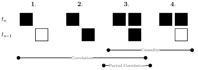
Figure 1: Visual representation of the four scenarios of restrictions on the values of the log returns and in which calculations are they used (bottom lines). In all four cases the left square denotes the leader, while the right one(s) correspond to the lagger. Full square denotes that only observations with nonzero value is considered, while empty one means that the log return which is used might have zero value as well.

The second case corresponds to the correlations obtained from the observations of simultaneous nonzero returns on the leader and the lagger in the next minute. Under such circumstances, one has an estimate on how much of the change of the price of the lagger, which certainly occurred, is possibly influenced by the previous return on the leader.

In order to calculate the partial correlation, in the third scenario we further specify the lagger to have nonzero return at the same minute as the leader. Such restriction is necessary for removal of the correlation between simultaneous returns of the leader and the lagger and the lagged autocorrelation of the latter, as potential contributors. This scenario was also used for determination of causal relationships.

In the last case we use observations of nonzero returns on the leader and lagger at the same minute, and apply it solely for identifying Granger causality. Under this scenario, one checks for predictability potential based on linear regression when one has two signals – simultaneous observations of nonzero values of the two relevant returns.

The collected data spans from January 2016 until December 2018. For computational reasons we calculated the quantities of interest for each of the 36 months separately. In representing the rankings, the averages of the monthly results are given.

Moreover, we point out that even though log returns are usually assumed to be weakly stationary, the empirical data may not exhibit such properties. This might be especially true for foreign exchange markets where the assets display extremely high dynamics and volatility. To statistically test whether the data used here is appropriate for studying lead-lag relationships that we are interested in, we utilize the Dickey-Fuller test [27]. This is a standard test used in time series analysis for examining the weak stationarity of a series. Under the null hypothesis, the test assumes that the time series under study has unit root. More precisely, we have applied augmented version of the test [28], where the difference of consecutive returns $\Delta r_{i}(t_{n})=r_{i}(t_{n})-r_{i}(t_{n-1})$ is regressed with the past return $r_{i}(t_{n-1})$, and the previous difference $\Delta r_{i}(t_{n-1})$. We could not examine lags of the difference of log returns of higher order because the presence of gaps in the data would decrease the number of samples where chains of consecutive differences are available. Correspondingly, this would weaken the statistical power of the test. Also, possible presence of time trend in the series was accounted for. To sum up, we have considered the following regression model

$$\Delta r_{i}(t_{n})=\alpha+\delta t_{n}+\theta r_{i}(t_{n-1})+\gamma_{1}\Delta r_{i}(t_{n-1})+\epsilon_{n},$$ (13)

where $\alpha$, $\delta$, $\theta$, and $\gamma_{1}$ are coefficients, and $\epsilon_{n}$ is the error term. Under the null hypothesis, $\theta=0$ suggests presence of unit root.

The Dickey Fuller test statistic calculated for each month in 2016 separately, and for all exchange rates is reported in the Table 2. Because the critical value of the test statistic for level 0.01 is -3.96 [29], one can observe that in each case the null hypothesis of presence of unit root can be rejected with high confidence. Accordingly, one can consider that the time series of log returns are weakly stationary.

Table 2: Dickey-Fuller test statistic (DFTS) for studied exchange rates in 2016

Rate	DFTS	Rate	DFTS	Rate	DFTS
AUD/CAD	-125.6	EUR/SEK	-113.8	USD/CAD	-121.8
AUD/CHF	-122.1	EUR/TRY	-117.0	USD/CHF	-122.5
AUD/JPY	-121.4	EUR/USD	-131.0	USD/CZK	-118.8
AUD/NZD	-126.3	FRX/EUR	-89.9	USD/DKK	-122.1
AUD/USD	-122.0	GBP/AUD	-123.8	USD/HKD	-49.2
AUX/AUD	-79.8	GBP/CAD	-123.7	USD/HUF	-111.1
BCO/USD	-96.4	GBP/CHF	-123.5	USD/JPY	-117.4
CAD/CHF	-122.6	GBP/JPY	-118.7	USD/MXN	-113.2
CAD/JPY	-120.4	GBP/NZD	-123.2	USD/NOK	-118.3
CHF/JPY	-118.5	GBP/USD	-120.5	USD/PLN	-116.3
ETX/EUR	-54.7	GRX/EUR	-92.5	USD/SEK	-125.5
EUR/AUD	-119.0	HKX/HKD	-83.8	USD/SGD	-116.4
EUR/CAD	-122.0	JPX/JPY	-68.9	USD/TRY	-103.1
EUR/CHF	-121.4	NSX/USD	-105.4	USD/ZAR	-111.4
EUR/CZK	-39.6	NZD/CAD	-123.7	WTI/USD	-98.4
EUR/DKK	-28.1	NZD/CHF	-122.6	XAG/USD	-108.9
EUR/GBP	-122.6	NZD/JPY	-121.1	XAU/AUD	-117.4
EUR/HUF	-91.2	NZD/USD	-121.0	XAU/CHF	-118.9
EUR/JPY	-117.7	SGD/JPY	-118.8	XAU/EUR	-118.7
EUR/NOK	-121.7	SPX/USD	-75.7	XAU/GBP	-102.1
EUR/NZD	-122.1	UDX/USD	-105.9	XAU/USD	-117.4
EUR/PLN	-101.8	UKX/GBP	-89.9	ZAR/JPY	-110.2

Finally, we point that here we have considered exchange rates as assets, instead of using values of currencies or commodities. To obtain the value of a currency one should quote it in terms of another one, taken as base, by using the appropriate exchange rate [30]. However, one does not always have a direct exchange rate between the appropriate base and any other currency in this market. In such cases two or more exchange rates might be needed for determination of the value of the asset. When many gaps in the data are present, or when some returns are inactive for certain period, getting such values can be problematic. Besides this, it has been found that the choice of basic currency can result in nontrivial difference in the obtained correlations [keskin2011topology, 30].

4 Results and discussion

4.1 Statistical significance of results

To determine statistical significance of the results, we applied the Bonferroni threshold correction. The Bonferroni correction is standardly used for handling situations when one makes multiple tests simultaneously, as is the case with the overall significance of the correlation matrix [31, 32]. For correlations between each of the $N$ assets the Bonferroni correction is $N\cdot N$. Thus, the appropriate threshold for $p$ value at level $0.01$, which is widely applied in the literature [32], is $0.01/(66\cdot 66)$. This threshold was applied for the two types of lagged correlations and for the Granger causality relationships.

4.2 Lagged correlations

As it was elaborated in Section 2.1, the lagged correlations quantify the relationship between series of one-minute log returns of two exchange rates with one of them trailing the other for a unit period. The existence of statistically significant correlation implies that the one with preceding returns presumably influences the other. We calculated such lagged correlations for all pairs in the dataset and summarized them in the respective $66\times 66$ correlation matrix. Due to the very intensive trading of the currencies, and highly dynamical nature of their values, most of the lagged correlations between exchange rates involving currencies do not pass the statistical significance tests. However, there are many nonzero terms in the lagged correlation matrix, notably those involving stock market indexes. As expected, the correlation matrix is asymmetrical because the influence is not identical in both directions. Out of this lagged correlation matrix we create a directed network where a link from node $j$ to $i$ exists if the rate $i$ has statistically significant correlation with $j$, and where $i$ is the leader.

In the second, third and fourth columns of Table 3 we present the ten most influential exchange rates on average, according to the PageRank for the three years under consideration and the three lagged correlation scenarios respectively. The results appear rather surprising, since market indexes with slower dynamics are put on top. This is opposite to previous findings where it was discovered that the more liquid assets lead the others [7, 8, 14]. In particular, the first four entries, all corresponding to such market indexes, appear rather high on the rank list nearly every month. The following ones, such as WTI oil exhibit varying influence in the lagged correlation matrix and are ranked rather differently in different months. The reason that the market indexes are most influential could be the fact that their price dynamics is slower and every change of their value incorporates some market news.

Table 3: Top ten most influential exchange rates in five cases: LC1, LC2 and LC3 – lagged correlations in scenarios 1, 2, and 3 respectively; LPC – most influential rates in lagged partial correlations; C1 and C2 – ranking of Granger causality significance in scenarios 3 and 4 respectively.

Rank	LC1	LC2	LC3	LPC	C1	C2
1	ETX/EUR	ETX/EUR	ETX/EUR	ETX/EUR	ETX/EUR	ETX/EUR
2	JPX/JPY	JPX/JPY	JPX/JPY	JPX/JPY	JPX/JPY	JPX/JPY
3	AUX/AUD	AUX/AUD	AUX/AUD	SPX/USD	SPX/USD	SPX/USD
4	SPX/USD	SPX/USD	SPX/USD	AUX/AUD	AUX/AUD	AUX/AUD
5	USD/CZK	USD/CZK	USD/CZK	WTI/USD	USD/CZK	USD/CZK
6	WTI/USD	WTI/USD	WTI/USD	USD/CZK	WTI/USD	WTI/USD
7	EUR/USD	USD/HUF	USD/HUF	NZD/USD	AUD/USD	AUD/USD
8	USD/HUF	ZAR/JPY	ZAR/JPY	AUD/USD	NZD/USD	UDX/USD
9	ZAR/JPY	EUR/USD	AUD/USD	USD/DKK	UDX/USD	NZD/USD
10	UDX/USD	UDX/USD	EUR/USD	BCO/USD	BCO/USD	USD/DKK

To validate whether some correlations are not a random result, but simply correspond to low influence, we also look at the results without the Bonferroni correction. The results for the statistically significant lagged correlations, which pass the threshold $p=0.01$ in each of the studied 36 months are displayed in Table 4. These results correspond to the first three scenarios. One can note that mostly the same correlations are present in the three situations. Only in few cases some additional correlation pairs appear when either the return in the leader is nonzero, or both the leader and the lagger in the next minute have nonzero returns. Although accidental emergence of correlation among $N$ uncorrelated time series with such significance threshold would not be a surprise, its appearance in 36 months consecutively suggests that some relationships between all such pairs really exist. From the same table one can notice some interesting patterns. First, dominant leaders are the same four stock market indexes AUX, ETX, JPX, and SPX, that appear as top sources of information spillover as detected with the PageRank. They influence the other indexes FRX, GRX, HKX, NSX, UKX and UDX. It is interesting that the other US-based index NSX is not as influential as the SPX. In addition, one can note that as laggers appear many exchange rates involving the Japanese Yen. When the above mentioned leading market indexes gain value, the Yen seems to react by weakening with respect to other assets. Another intriguing observation is the lowering of the value of gold ounce, XAU, quoted in AUD, when these indexes rise. One can also note that rise or fall of the MXN with respect to the US dollar, is followed by similar behavior of the TRY. These two minor currencies have been also found to be mutually related in a previous study [30]. Finally, it is interesting that the fall of the MXN with respect to the USD, is followed by similar behavior of the ZAR with respect to the JPY.

Table 4: Persistent statistically significant correlations.

Leader	Positively correlated lagger
AUX/AUD	AUD/JPY, CAD/CHF, CAD/JPY, FRX/EUR,
	GRX/EUR, HKX/HKD, NSX/USD, NDZ/JPY,
	SGD/JPY, SPX/USD, UDX/USD, UKX/GBP,
	USD/JPY
ETX/EUR	AUD/JPY, CAD/JPY, FRX/EUR, GBP/JPY,
	GRX/EUR, HKX/HKD, NSX/USD, NDZ/JPY,
	SGD/JPY, SPX/USD, UDX/USD, UKX/GBP,
	USD/JPY
JPX/JPY	AUD/JPY, CAD/CHF, CAD/JPY, CHF/JPY3,
	EUR/JPY, FRX/EUR, GBP/JPY, GRX/EUR,
	HKX/HKD, NSX/USD, NDZ/JPY, SGD/JPY,
	SPX/USD3, UDX/USD, UKX/GBP, USD/JPY
SPX/USD	AUD/JPY, CAD/JPY, SGD/JPY3
USD/MXN	USD/TRY
Leader	Negatively correlated lagger
AUD/USD	USD/TRY
ETX/EUR	XAU/AUD
JPX/JPY	XAU/AUD
SPX/USD	XAU/AUD
USD/MXN	ZAR/JPY4

4.3 Lagged partial correlations

We quantify the importance of the exchange rates as determined from the lagged partial correlations through the PageRank algorithm, as well. In the fifth column of Table 3, we show the ranking of the most influential exchange rates. The same four major market indexes, as in the lagged correlation case, appear at the top of the rankings. When applying the ordinary critical value of $0.01$ instead of the Bonferroni correction we find similar results as in the previous section. These results are provided in Table 5. However, these results also suggest why at the top is the European stock market index ETX. Namely, the log returns on it, lead the returns of all market indexes AUX, FRX, GRX, HKX, JPX, NSX, SPX, and UKX. It is influenced by the FRX and GRX, which is a feedback relationship, something that was not present in the ordinary correlations. This influence is not symmetrical and is more pronounced from the ETX towards FRX and GRX, than in the opposite direction.

We find that other bidirectional partial correlations are those between the two oil brands, and between TRY and ZAR when quoted in US dollars. We remark that in the ordinary case, these currencies did not possess any mutual lagged correlation. Moreover, our results show that the value of TRY and ZAR in US dollars seems to be also similar in their trailing of the dynamics of the two Oceanic currencies AUD and NZD as quoted in the USD. The returns on AUD/USD also show sign of having some influence on those on SGD/USD. Particularly important is the fact that the return on the silver in USD, precedes similar behavior of the gold in the next minute. In a related observation involving precious metals, it appears that the CHF adjusts its value in terms of gold, after the neighboring EUR has done it one minute before. When any of the MXN, TRY, or ZAR gains its value in USD, ZAR is induced to behave similarly with respect ot the JPY. Also, it is likely that the MXN has some influence on the ZAR which was not observed from the ordinary lagged correlations. Finally, interesting observations are those involving currencies from the Eurozone. The value of PLN in USD seems to influence the HUF quoted in the same currency base. It is also peculiar that the value of the minor currency CZK given in terms of US dollars, influences the major EUR, but not the opposite.

4.4 Granger causality

The tests for presence of Granger causality were performed under scenarios 3 and 4, where both the leader and lagger must have nonzero returns simultaneously, while in scenario 3 additionally the lagger also needs to have non-vanishing returns in two consecutive periods. The statistically significant causal relationships were presented in a directed network and the importance of exchange rates was again determined with the PageRank algorithm. We note that the networks which we have considered for depicting the causal relationships are not weighted, which means that a link between two pairs exists only if the source node is influenced by the target node, and the weight of each such link is one. As expected, the rates involving market indexes appear at the top of the list. The rankings of ten rates with strongest causal influence are provided in the last two columns in table 3, where similar ordering with the other two measures (lagged correlations and lagged partial correlations) is observed. Clearly, it can be argued that the lagged correlations, both partial and ordinary, suggest that a causal relationship is present between a leader and its lagger. By lowering the threshold for statistical significance to $0.01$, as in previous cases, we obtain almost the same pairs of exchange rates as in the case of partial correlations. The only exception is the existence of statistically significant partial lagged correlation between the JPX/JPY as leader and the CHF/JPY. The causality relationships under both scenarios between the same pair does not pass the threshold for only one month, December in 2017. This might be result of statistical nature and one could speculate that both scenarios produce the same results.

We state that one might be suspicious in the predictability under scenario 3, where we determine causality when the lagger is constrained to have nonzero return in the next minute. However, in the weaker case, when non-vanishing returns of the leader and the lagger are observed simultaneously, one can use them as signals, and make a regression on the future value of the return on the lagger.

Table 5: Persistent statistically significant partial correlations and causality relationships.

Leader	Same direction
AUX/AUD	AUD/JPY, CAD/CHF, CAD/JPY, FRX/EUR,
	GBP/JPY, GRX/EUR, HKX/HKD, NSX/USD,
	NDZ/JPY, SGD/JPY, SPX/USD, UDX/USD,
	UKX/GBP, USD/JPY, ZAR/JPY
BCO/USD	WTI/USD
ETX/EUR	AUD/JPY, AUX/AUD, CAD/CHF, CAD/JPY,
	FRX/EUR, GBP/JPY, GRX/EUR, HKX/HKD,
	JPX/JPY, NSX/USD, NDZ/JPY, SGD/JPY,
	SPX/USD, UDX/USD, UKX/GBP, USD/JPY
FRX/EUR	ETX/EUR, GRX/EUR
GRX/EUR	ETX/EUR
JPX/JPY	AUD/JPY, CAD/CHF, CAD/JPY, CHF/JPY ,
	EUR/JPY, FRX/EUR, GBP/JPY, GRX/EUR,
	HKX/HKD, NSX/USD, NDZ/JPY, SGD/JPY,
	SPX/USD, UDX/USD, UKX/GBP, USD/JPY
SPX/USD	AUD/JPY, CAD/JPY, GRX/EUR, NSX/USD,
	NZD/JPY, SGD/JPY, UDX/USD
USD/CAD	USD/ZAR
USD/MXN	EUR/TRY, USD/TRY, USD/ZAR
USD/PLN	USD/HUF
USD/TRY	USD/ZAR
USD/ZAR	EUR/TRY, USD/TRY
WTI/USD	BCO/USD
XAG/USD	XAU/USD
XAU/EUR	XAU/CHF
ZAR/JPY	SGD/JPY
Leader	Opposite direction
AUD/USD	USD/SGD, USD/TRY, USD/ZAR
AUX/AUD	XAU/AUD
ETX/EUR	XAU/AUD
JPX/JPY	XAU/AUD
NZD/USD	USD/TRY, USD/ZAR
SPX/USD	XAU/AUD
USD/CZK	EUR/USD
USD/MXN	ZAR/JPY
USD/TRY	ZAR/JPY
USD/ZAR	ZAR/JPY
ZAR/JPY	EUR/TRY

Since the foreign exchange is known to be very liquid, one can not expect significant lags that span longer than one minute. To empirically check this hypothesis we also made an analysis where we examine whether these lagged relationships persist for longer periods. For this purpose we re-estimated our metrics for lead-lag relationships by taking into account for lagger returns that trail two minutes. We found that there are some pairs of exchange rates that pass the significance threshold of 0.01. However, they are not consistent. In particular, no such pair passed the test for all months in 2016. This is a further indication that the relevant lagging time scale is of order of one minute. Due to spatial constraints, we do not show these results, but make them available upon request.

5 Conclusions

To conclude, here we studied the relations between pairs of exchange rates where one exchange rate lags the other for one minute, and considered three different approaches. The first one considers lagged correlations which quantify similarity of log returns between lead and lagged exchange rate. The second approach restricts the lagged correlations to partial, in order to account for the potential autocorrelation. Finally, the last approach tries to uncover the causal relationships in the foreign exchange market in the sense of Granger.

The existence of statistically significant lagged correlations shows that, even though, the foreign exchange market is known to have very fast dynamics, information spreading is not instantaneous. We discovered that the rates which cause others to follow their dynamics are mostly those which involve stock market indexes. Observing changes in the value of an index, implies that certain currencies, or market indexes would more likely gain, while others would loose value. This was further confirmed by the calculation of the lagged partial correlation between the leader and the lagger exchange rate. By applying the PageRank algorithm on the statistically significant correlations in both cases we found that the most influential rates are indeed those involving market indexes. The same conclusions hold even when we estimated the Granger causality between pairs of exchange rates. When lagging period is two minutes, these lead-lag effects disappear, which suggests that the typical lagging time is of the order of one minute.

In spite of the fact that the existence of lagged correlations and causality challenges the efficient market hypothesis in foreign exchange markets, we are still uncertain of the existence of arbitrage. In order for this phenomenon to be proven, one should verify whether the potential statistical-arbitrage-based profit can overcome the transaction costs. Investigating the presence of arbitrage should be a topic of future research which, besides the bid quotes, requires additional information such as ask price, transaction costs and time needed to complete the transaction.

As a final remark, we state that here we did not investigate the temporal dynamics of the discovered correlation patterns. A more detailed study which captures the dependencies among these temporal correlations could reveal novel insights for the nature of the lead-lag relationships in foreign exchange markets.

6 Acknowledgement

We are grateful to histdata.com for freely sharing their data. This research was partially supported by the Faculty of Computer Science and Engineering at “SS. Cyril and Methodius” University in Skopje, Macedonia and by DFG through grant “Random search processes, Lévy flights, and random walks on complex networks”.

References

- [1] Vasiliki Plerou, Parameswaran Gopikrishnan, Bernd Rosenow, Luís A Nunes Amaral, and H Eugene Stanley. Universal and nonuniversal properties of cross correlations in financial time series. Phys. Rev. Lett., 83(7):1471, 1999.
- [2] Rosario N Mantegna. Hierarchical structure in financial markets. Eur. Phys. Jour. B, 11(1):193–197, 1999.
- [3] Takayuki Mizuno, Hideki Takayasu, and Misako Takayasu. Correlation networks among currencies. Phys. A, 364:336–342, 2006.
- [4] Michael J Naylor, Lawrence C Rose, and Brendan J Moyle. Topology of foreign exchange markets using hierarchical structure methods. Phys. A, 382(1):199–208, 2007.
- [5] Mehmet Eryiğit and Resul Eryiğit. Network structure of cross-correlations among the world market indices. Phys. A, 388(17):3551–3562, 2009.
- [6] Burton G Malkiel and Eugene F Fama. Efficient capital markets: A review of theory and empirical work. J. Finance, 25(2):383–417, 1970.
- [7] Ira G Kawaller, Paul D Koch, and Timothy W Koch. The temporal price relationship between s&p 500 futures and the s&p 500 index. J. Finance, 42(5):1309–1329, 1987.
- [8] Andrew W Lo and A Craig MacKinlay. When are contrarian profits due to stock market overreaction? Rev. Financ. Stud., 3(2):175–205, 1990.
- [9] Nicolas Huth and Frédéric Abergel. High frequency lead/lag relationships—empirical facts. J. Empir. Finance, 26:41–58, 2014.
- [10] Lisi Xia, Daming You, Xin Jiang, and Wei Chen. Emergence and temporal structure of lead–lag correlations in collective stock dynamics. Phys. A, 502:545–553, 2018.
- [11] Sebastien Valeyre, Denis S Grebenkov, and Sofiane Aboura. Emergence of correlations between securities at short time scales. Phys. A, 526:121026, 2019.
- [12] Thong Minh Dao, Frank McGroarty, and Andrew Urquhart. Ultra-high-frequency lead–lag relationship and information arrival. Quant. Finance, 18(5):725–735, 2018.
- [13] Clive WJ Granger. Investigating causal relations by econometric models and cross-spectral methods. Econometrica, pages 424–438, 1969.
- [14] Bence Tóth and János Kertész. Increasing market efficiency: Evolution of cross-correlations of stock returns. Phys. A, 360(2):505–515, 2006.
- [15] Sergey Brin and Lawrence Page. The anatomy of a large-scale hypertextual web search engine. Computer networks and ISDN systems, 30(1-7):107–117, 1998.
- [16] Scott White and Padhraic Smyth. Algorithms for estimating relative importance in networks. In Proceedings of the ninth ACM SIGKDD international conference on Knowledge discovery and data mining, pages 266–275. ACM, 2003.
- [17] Nan Ma, Jiancheng Guan, and Yi Zhao. Bringing pagerank to the citation analysis. Information Processing & Management, 44(2):800–810, 2008.
- [18] Matthew E Falagas, Vasilios D Kouranos, Ricardo Arencibia-Jorge, and Drosos E Karageorgopoulos. Comparison of scimago journal rank indicator with journal impact factor. The FASEB journal, 22(8):2623–2628, 2008.
- [19] Filippo Radicchi. Who is the best player ever? a complex network analysis of the history of professional tennis. PloS one, 6(2):e17249, 2011.
- [20] Jianqing Fan and Qiwei Yao. The elements of financial econometrics. Cambridge University Press, 2017.
- [21] Kunihiro Baba, Ritei Shibata, and Masaaki Sibuya. Partial correlation and conditional correlation as measures of conditional independence. Aust. N Z J Stat., 46(4):657–664, 2004.
- [22] Dror Y Kenett, Michele Tumminello, Asaf Madi, Gitit Gur-Gershgoren, Rosario N Mantegna, and Eshel Ben-Jacob. Dominating clasp of the financial sector revealed by partial correlation analysis of the stock market. PloS one, 5(12):e15032, 2010.
- [23] Dror Y Kenett, Xuqing Huang, Irena Vodenska, Shlomo Havlin, and H Eugene Stanley. Partial correlation analysis: Applications for financial markets. Quant. Finance, 15(4):569–578, 2015.
- [24] Yong Mai, Huan Chen, Jun-Zhong Zou, and Sai-Ping Li. Currency co-movement and network correlation structure of foreign exchange market. Phys. A, 492:65–74, 2018.
- [25] Michele Tumminello, Tomaso Aste, Tiziana Di Matteo, and Rosario N Mantegna. A tool for filtering information in complex systems. PNAS, 102(30):10421–10426, 2005.
- [26] Helmut Lütkepohl. New introduction to multiple time series analysis. Springer Science & Business Media, 2005.
- [27] David A Dickey and Wayne A Fuller. Distribution of the estimators for autoregressive time series with a unit root. Journal of the American statistical association, 74(366a):427–431, 1979.
- [28] Jeffrey M Wooldridge. Introductory econometrics: A modern approach. Nelson Education, 2015.
- [29] Wayne A Fuller. Introduction to statistical time series, volume 428. John Wiley & Sons, 2009.
- [30] Lasko Basnarkov, Viktor Stojkoski, Zoran Utkovski, and Ljupco Kocarev. Correlation patterns in foreign exchange markets. Phys. A, 525:1026–1037, 2019.
- [31] Michele Tumminello, Salvatore Micciche, Fabrizio Lillo, Jyrki Piilo, and Rosario N Mantegna. Statistically validated networks in bipartite complex systems. PloS One, 6(3):e17994, 2011.
- [32] Chester Curme, Michele Tumminello, Rosario N Mantegna, H Eugene Stanley, and Dror Y Kenett. Emergence of statistically validated financial intraday lead-lag relationships. Quant. Finance, 15(8):1375–1386, 2015.