AC Oscillation of a Spin Soliton Driven by a Constant Force
Abstract
The phenomena of AC oscillation generated by a DC drive, such as the famous Josephson AC effect in superconductors and Bloch oscillation in solid physics, are of great interest in physics. Here we report another example of such counter-intuitive phenomenon that a spin soliton in a two-component Bose-Einstein condensate is driven by a constant force: The initially static spin soliton first moves in a direction opposite to the force and then changes direction, showing an extraordinary AC oscillation in a long term. In sharp contrast to the Josephson AC effect and Bloch oscillation, we find that the nonlinear interactions play important roles and the spin soliton can exhibit a periodic transition between negative and positive inertial mass even in the absence of periodic potentials. We then develop an explicit quasiparticle model that can account for this extraordinary oscillation satisfactorily. Important implications and possible applications of our finding are discussed.
The phenomena of AC oscillation generated by a DC drive are of great interest because of their counter-intuitive character Barone ; Makhlin ; bloch ; blochuse . The Josephson AC effect is the famous one. It was first predicted in the context of electron tunneling across an insulating barrier between two superconductors Jose , in which a unidirectional driving voltage can result in oscillating electronic currents. The underlying mechanism is quantum phase coherence. The Bloch oscillation in solid physics is another example, which describes the motion of an electron in a periodic potential driven by a DC electric field BO ; BO2 . It is a direct consequence of the periodicity of the energy band structure that can induce a transition between the negative effective mass and positive massDahan . These striking phenomena not only are interesting in physics but also have important applications. For instance, a superconducting quantum interference device (SQUID) based on the Josephson effect has been invented that is extremely sensitive to magnetic measurements squid .
In this paper, we report that a spin soliton in a cigar-shaped two-component Bose-Einstein condensate (BEC) can also demonstrate the AC oscillation in the presence of an external unidirectional constant force. The oscillation frequency is proportional to the force, and the amplitude is inversely proportional to the force. The underlying mechanism, however, is distinct from the phase-coherent mechanism of a typical Josephson oscillation in superconductors Jose and many other Josephson-like oscillations in various quantum systems Liu ; Levy ; Polo ; Cataliotti ; Valtolina . We find that the inertial mass of the spin soliton can exhibit a periodic transition between negative and positive values because of a particular relation between its energy and moving velocity. This is somewhat similar to what occurs in the Bloch oscillation BO ; BO2 ; Dahan ; however, the periodic potential is absent and the nonlinear interactions between the degenerate atoms play an important role in our situation. This inertial mass transition effect implies that the spin soliton can sometimes accelerate along the force direction and sometimes accelerate in the opposite direction, leading to an AC oscillation. We then develop a quasiparticle model to describe the motion of the spin soliton that can quantitatively account for this extraordinary oscillation. An experimental observation, important implications and a possible application to weak force measurements are discussed.
Spin solitons in a two-component BEC. We consider a two-component BEC system which is tightly confined in the radial direction so that the radial characteristic length is smaller than the healing length and its dynamics is essentially one-dimensional (1D) Kevrekidis . Rescaling the atomic mass and Planck’s constant to be , the mean-field energy for the quasi-1D BEC system can be written as Kevrekidis . is the axial coordinate, and denotes the condensate wave function, where refers to the two components. The dimensionless dynamical equations can be written as the following coupled model,
| (1) | |||
| (2) |
The parameters and denote intraspecies interactions between the atoms in the components and , respectively, and describes the interspecies interactions between the atoms.
For , the system is described by an integrable Manakov model Mana , and various types of solitons have been deduced using the traditional inverse scattering method, Bäcklund transformation method and Hirota bilinear method Mat ; Hirota ; Zhao ; Lingdnls , such as bright-bright, bright-dark, and dark-dark solitons. Nevertheless, these solutions cannot be extended to non-Manakov cases where the constraint condition is not satisfied. Here, we claim that under the conditions of and , we can derive an exact soliton solution with a the constraint condition ( for simplicity, see Appendix A for details). A soliton solution with , as an example, can be written in the following explicit form:
| (3) | |||||
| (4) | |||||
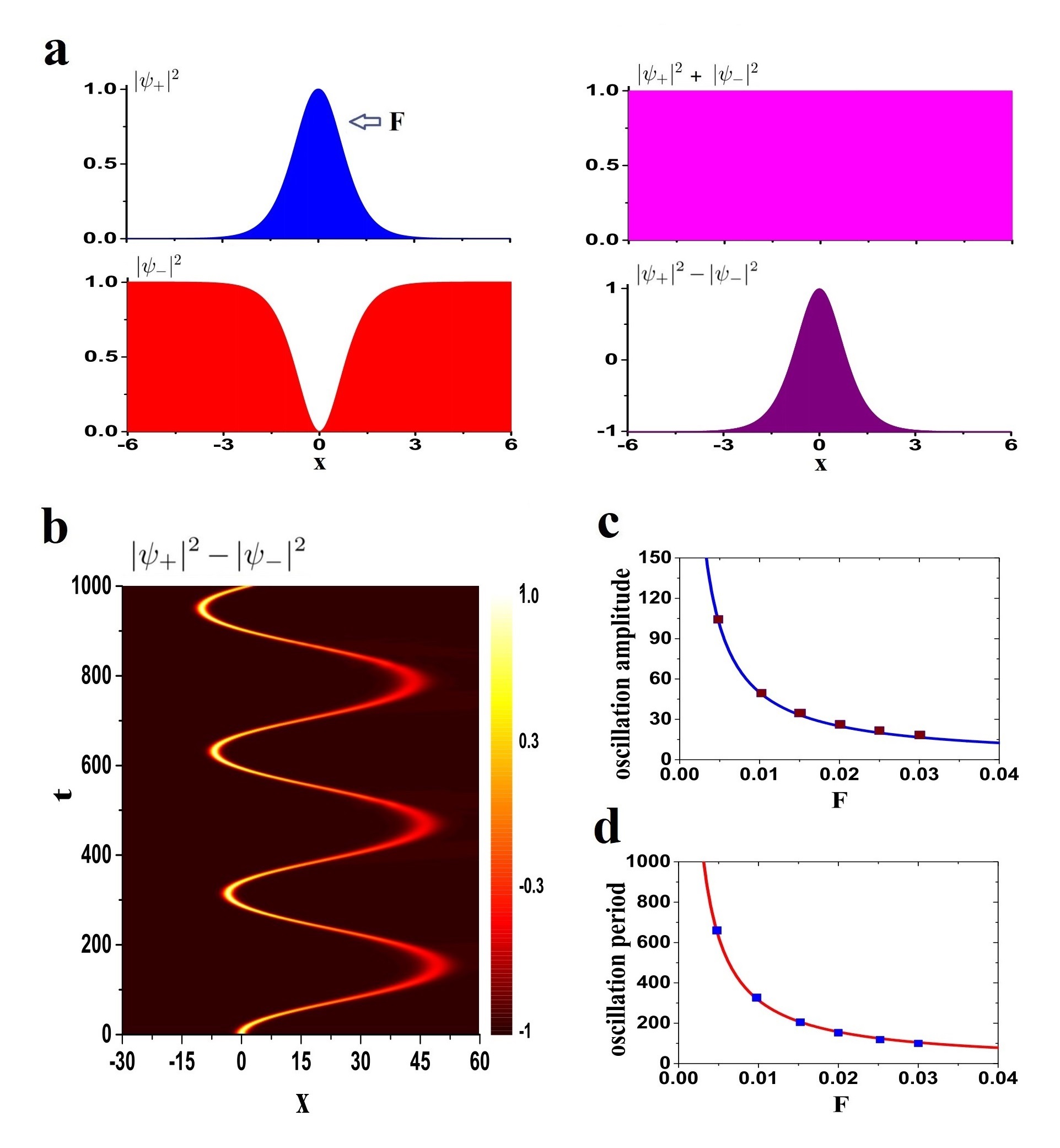
where denotes the maximum speed of soliton. The moving velocity of the soliton should be smaller than , and when it equals the speed of sound, the above solution degenerates to a plane wave. When , we have a static soliton, as shown in Fig. 1 (a). The particle density in the () component admits a bright soliton (dark soliton). The bright soliton in one component is induced by the effective potential generated by the dark soliton in the other component Carr .
The total density distribution of the soliton solution is uniform, i.e., , while the population imbalance of ranged in exhibits an explicit soliton profile. This differs from that of the usual dark-bright solitons reported previously, where the sum density distribution also shows a soliton profile Busch ; Nistazakis ; Carr ; BEC ; Hamner . For each position, the solution has the analogous structures of a spin-half system represented by a Bloch sphere pspin ; Liu2 ; Liu3 ; Liu4 ; Liu5 , therefore, we term it as spin soliton. A linear stability analysis has indicated that the spin soliton is stable (see Appendix B). Note that the spin soliton emerges in the phase separation regime with , the background densities of its two components are different and equal to zero and unit, respectively. In contrast, for the “magnetic soliton” found very recently Qu , the background densities of its two components have the same value of with a unit total density background. It has the character of phase miscibility and emerges in the regime of .
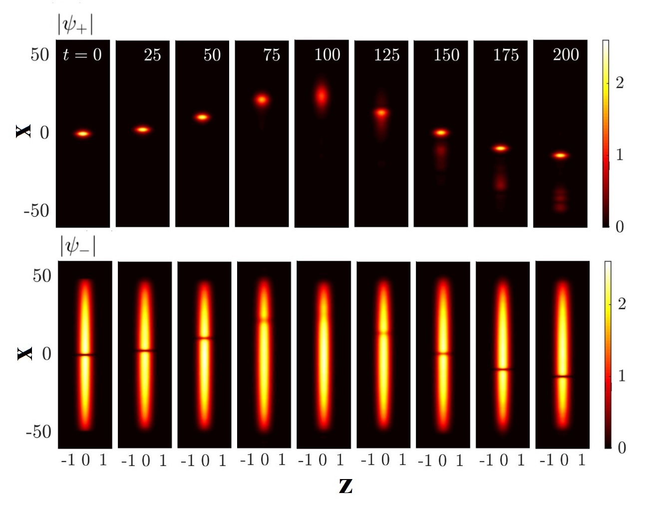
The AC oscillation of a spin soliton. We now investigate the dynamics of the spin soliton driven by a constant force. Initially, the spin soliton is set to be static, as shown in Fig. 1 (a). A weak unidirectional force (sketched by Fig. 1 (a)) or, equivalently, a linear potential , is added only to the bright soliton component to avoid accelerating the whole particle density background. In simulations, a term of is added to the mean-field energy. Here, “weak” means that the external potential varies slowly over the size scale of the soliton Busch ; therefore, it cannot destroy the soliton structure. We solve the nonlinear Schrödinger equation numerically in a spatial range of by the discrete Cosine transform method with homogeneous Neumann boundary conditions Yang ; Tang .
We chose to demonstrate our results. Strikingly, the spin soliton moves in a direction opposite to the force for a while and then changes direction, showing an oscillation over the long term, as shown by the spin density evolution in Fig. 1 (b). During the evolution, the whole particle density remains almost uniform with only an approximately mass density fluctuation. We perform further numerical calculations to investigate the dependence of the oscillation amplitude and period on external force . The results are shown in Fig. 1 (c) and (d), respectively. It is clearly shown that the oscillation frequency is proportional to the force and the amplitude is inversely proportional to the oscillation frequency.
Our extensive simulations show that the oscillation behavior can emerge even for a bit higher or lower bright soliton component, when the force strength is smaller than . We have tuned the coupling strengths by in absolute magnitudes deviated from and , the AC oscillation still can be observed clearly. It indicates that the striking oscillation phenomenon is rather robust.
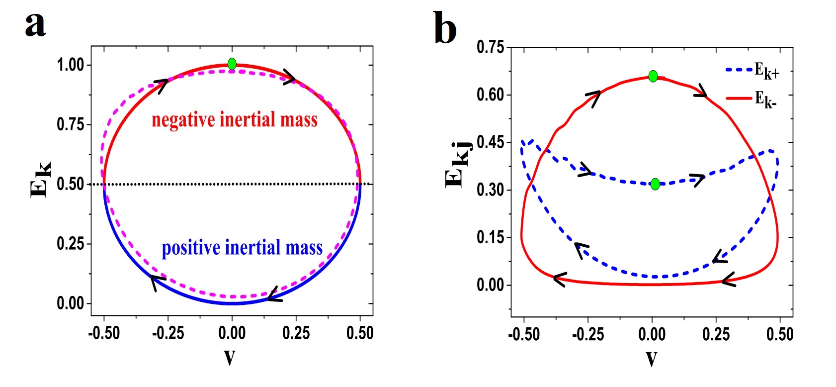
Negative-positive mass transition. To understand this striking oscillation behavior, we first investigate the kinetic energy of the spin soliton. The exact spin soliton solution of the explicit expressions (3-4) cannot describe the acceleration process because, in the presence of an external force, the spin soliton will evolve with a broadening or shrinking of its width and change shape. Thus, we have to calculate the kinetic energy of the spin soliton (the interaction energy keeps nearly zero for a spin soliton) by directly solving the nonlinear Schrödinger equation according to . The parameter is chosen to be a bit larger than the soliton size, i.e., and . Our extensive numerical calculations suggest a simple approximate relation between the kinetic energy and moving velocity of note1 , which gives two branches of , as shown in Fig. 2 (a). This explicit dispersion relation is further verified analytically according to the Lagrangian variational method (see Appendix C for details).
The density profile of the spin soliton is spatially localized during the whole evolution (see Fig. 1 (b)); therefore, the spin soliton can be viewed as a quasiparticle. The inertial mass of the spin soliton can be derived from the relation between the soliton energy and velocity according to Brand , i.e.,
| (5) |
The inertial mass of the spin soliton is shown in Fig. 2 (a). It is seen that the spin soliton admits both negative mass (upper semicircle) and positive mass (lower semicircle) during each oscillation period.
We also calculate the inertial mass for the dark soliton and bright soliton separately according to the individual kinetic energy in each component of the BEC. The results are shown in Fig. 2 (b). The relations also agrees well with the ones given by Lagrangian method. We see that the bright soliton admits positive inertial mass, and the dark soliton admits mainly negative mass, similar to scalar soliton systems Lewenstein ; PNAS . However, in contrast to a scalar soliton, the density profile of the bright soliton obtained here depends on the moving velocity, and its inertial mass varies with the velocity accordingly (see the blue dashed line in Fig. 2(b)). The dark soliton (red solid line in Fig. 2(b)), however, might exhibit positive mass around the maximum velocities.
When applying an external force, the bright soliton initially tends to move along the direction of the force. At same time, it drags the dark soliton to move along the force direction because the interaction between the dark soliton and bright soliton is indeed attractive due to the repulsive interaction between the two components. However, the dark soliton admits a relatively larger negative mass, implying that it prefers to move against the drag force (i.e., buoyancy effect) and can dominate the initial motion direction of the spin soliton. In the following temporal evolution, due to the interplay between the bright and dark solitons, the total inertial mass of the spin soliton can periodically change from negative to positive values. In contrast to the oscillation behavior of the magnetic soliton that is directly induced by the axial harmonic trap potential Qu , the striking oscillation of our spin soliton emerges in the absence of axial trapping potential and is due to the intrinsic mechanism of positive-negative mass transition.
Negative mass is an interesting subject Bondi ; Kromer ; Bonnor and is even believed to play an important role in the expansion of the early universe. Negative mass has also been reported in BEC systems. Recently, an experimental observation of negative mass effects was realized through the engineering of the dispersion relation by spin-orbit coupling effects negativemass , in which negative mass leads to dynamical instability and a sudden increase in the atomic density. Recently, interactions of solitons with positive and negative masses were investigated in a BEC trapped by an optical-lattice potential Sakaguchi .
Quasiparticle model. The concept of the inertial mass captures the response of the spin soliton to an applied force, encapsulating Newton’s equations of quasiparticle dynamics. The external potential energy of a soliton ( denotes the soliton center position). The force acting on the spin soliton is then . Thus, the dynamical trajectory of the spin soliton should be governed by . Let us consider the explicit expression of the inertial mass (5) and set the initial conditions to . The analytical solution of the above Newton equation is readily obtained as follows:
| (6) |
We can see that the oscillation amplitude and period , which agrees well with numerical simulations (see Fig. 1 (c) and (d)).
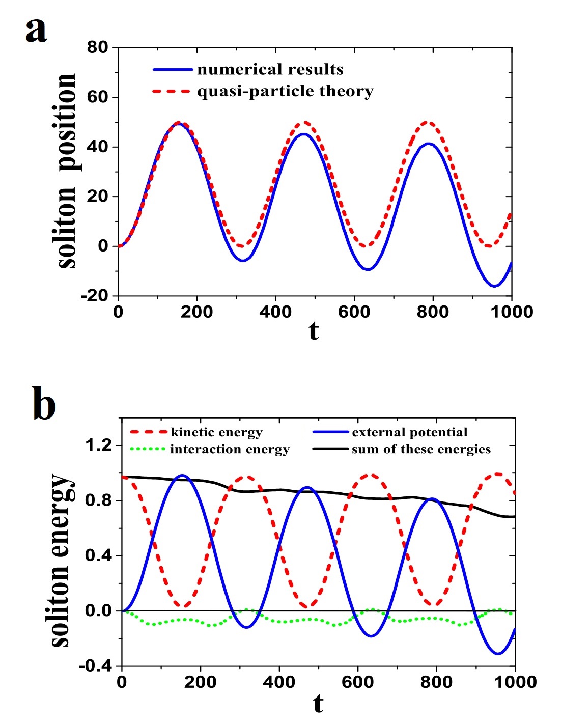
We have compared the theoretical prediction with numerical simulations for the AC oscillation in Fig. 1 (b). As shown in Fig. 3 (a), both the oscillation amplitude and period can be well predicted by the simple model, except for a small downward shift in the trajectory. To understand this deviation, in Fig. 3 (b), we integrate over the local soliton profile (safely in regime) and plot the temporal evolution of the kinetic energy , external potential energy , interaction energy of soliton Carr ; Kivshar , and sum of these energies. Compared to the other two types of energy, the total interaction energy sum over three terms keeps nearly zero, while each of them is not. Note that the interaction plays an important role manifesting that the dispersion relation or inertial mass are explicitly dependent on the interaction parameters. The kinetic energy oscillates periodically, and there is a periodic transition between the kinetic energy and external potential energy. However, the external potential energy shifts downward, and the energy sum shows an “unphysical” decay. These effects are due to the soliton energy spreading to other regimes through the excitation of dispersive waves or other nonlinear waves. Our numerical simulations indicate that dispersive waves mainly emerge in the dark soliton component and are almost absent in the bright soliton component. The total energy in the full space is conserved in our numerical simulations. Due to total energy conservation, with an increase in the dispersive wave energy, the external potential energy of the soliton will decrease, leading to a deviation in the spin soliton trajectory from our quasiparticle model.
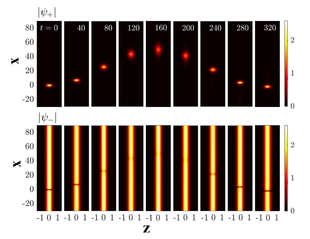
The AC oscillation in 3D setting. We now extend to investigate the AC oscillation in three-dimensional (3D) setting, that is, the BECs are trapped by a harmonic trap . Here, we use a strongly confining transverse frequency to ensure that radial characteristic length is smaller than the healing length for quasi-1D approximation (radial characteristic length is , and the healing length is about in this case). We will show that the striking AC oscillation emerges and is rather robust in the genuinely 3D situation. The 3D dynamical equations and simulation methods are given Appendix D.
We first set corresponding to the above quasi-1D BEC, the results presented in Fig. 4 demonstrate a perfect one cycle oscillation (see the movie dbmv for a more complete dynamics to ). The oscillation period () agrees to its 1D counterpart as well as our theory.
When , i.e., a harmonic trap along the -axis presents, we have still observed a kind of periodic oscillation shown in Fig. 5 (see the movie dbmv2 for a more complete dynamics to ). Its period is about , which is however much shorter than the one in Fig. 4. In this situation, the intrinsic AC oscillation has been dramatically influenced by the external potential. One can see some smear of the bright soliton component in Fig. 5, due to the nonlinear excitation generated by the external harmonic trap. Therefore, to observe our intrinsic AC oscillation, the external trap should be weak enough satisfying the limitation .
Discussion. We demonstrate that AC oscillation emerges for a driven spin soliton in a two-component BEC and reveal its distinctive mechanism associated with the negative-positive mass transition. Our numerical simulations indicate that spin soliton and the AC oscillation are stable and robust and can emerge in genuinely 3D situation. This striking phenomenon is expected to be observed in current experiments.
Let us consider ultra-cold atoms prepared in the internal states and (denoted by and , respectively). For hyperfine states, the scattering lengths can be manipulated by external magnetic fields Widera ; Tojo ; Mertes , which can be used to ensure that the nonlinear interaction strength nearly satisfies the condition for spin solitons. Recent experiments indicated that vector solitons can be prepared well in BEC systems BEC ; Hamner ; Bersano . Our numerical simulation also indicates that the AC oscillation phenomenon of a spin soliton is robust against a low level of noise and some parameter deviations from ideal condition. A weak magnetic field can be applied along the principal axis of the cigar-shaped BEC to drive the bright soliton in the state without influencing the component.
In principle, the AC oscillation phenomenon of a spin soliton can be used to diagnose weak forces or related physical quantities through a direct measurement of the moving period of ultracold atoms, for instance, the cigar-shaped BEC with a spin soliton could serve as a bubble level instrument that can work in a microgravity environment. This approach offers an alternative to the approach employed in recent experiments with optomechanical systems Schreppler ; Moller , where forces are determined through the measurement of optical frequencies.
Acknowledgments
Stimulating discussions with Xi-Wang Luo, and Jun-Peng Cao are acknowledged. Zhao is grateful to Ling-Zheng Meng and Peng Gao for their help in numerical simulations. This work is supported by the National Natural Science Foundation of China (Contract No. 11775176, 11775030, 11674034, U1930403), the Major Basic Research Program of Natural Science of Shaanxi Province (Grant No. 2018KJXX-094), and the Key Innovative Research Team of Quantum Many-Body Theory and Quantum Control in Shaanxi Province (Grant No. 2017KCT-12). W.W. acknowledges support from the Swedish Research Council Grant No. 642-2013-7837, and the Goran Gustafsson Foundation for Research in Natural Sciences and Medicine, and the Fundamental Research Funds for the Central Universities, China.
Appendix A: The method of deriving exact soliton solution
To obtain spin solitons, we firstly set a constrain condition on the mass density distributions . With this condition, we can further simplify the Eq. (1) and (2) as follows,
| (7) |
If and are both negative or positive, there are dark solitons or bright solitons in the two components. Obviously, the superposition of them can not be unform at all. Therefore, we need the second constrain condition that and have different signs for spin solitons. In this case, there are one dark soliton and one bright soliton in the two components respectively, and it is possible to satisfy the condition . We choose and to derive spin solitons analytically and exactly, from the well-known results of scalar nonlinear Schrdinger equation. Then, we can give static bright soliton and dark soliton solution of Eq. (7) as follows
| (8) |
where and determine the amplitude of bright soliton and plane wave background for dark soliton component respectively. Finally, the constrain condition further gives that , and . In this way, we construct a static spin soliton solution of Eq. (1) and (2) as follows
| (9) |
where denotes the speed of sound. One can derive spin soliton solution with velocity in similar ways, and the spin soliton solution is given in the text. This means that it is possible to construct exact spin soliton solutions with the condition . It should be noted that the spin soliton solutions fails to hold for the case , for which the coupled model becomes the well-known integrable Manakov model, and mass solitons exist with many different forms.
Appendix B: The stability of spin soliton in 1D
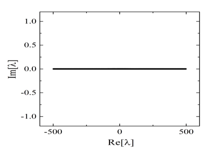
We perform linear stability analysis on the spin soliton. Introducing weak perturbations on the spin soliton, , (where and are the spin soliton solution), we can obtain linearized equation for the eigenvalue of . The excitation spectrum is shown in Fig. 6. indicates that spin soliton is stable. Numerical simulations also indicate that spin soliton is indeed robust against noises in one dimension case.
Appendix C: The analytic derivation of the relation between soliton energy and velocity by Lagrangian variational method
The dynamical equation of a two-component BEC driven by a constant force can be written as follows,
| (10) |
With considering the constrain condition , i.e., we can simplify Eq. (10) as follows,
| (11) |
where . The above equation can be further written as:
| (12) |
where , which are introduced to simplify the following calculations.
In the presence of the force term, the system become non-integrable and the exact analytic expressions for the dynamic evolution of the spin solitons can not be obtained. We thus exploit the Lagrangian variational method to evaluate the dynamics of the spin soliton by introducing the following trial functions,
| (13) | |||||
Note that the total density keeps a constant in temporal evolution. The soliton position, amplitudes and width vary in time.
We now use the Lagrangian variational method to derive expressions of . The Lagrangian of the system is: . The factor is introduced for the dark soliton state, or it is impossible to integrate the term . This problem was firstly solved by Yuri S. Kivshar et al. in 1995 Kivshar . It should be noted that is kept for spin soliton. Substituting the trial wavefunctions into the Lagrangian, and after taking the particularly elaborate integrals, we obtain that , where , etc. Our initial conditions are , . From the conservation of the norm of the bright component, we have . It is now straightforward to apply the Lagrangian equation , where . We have obtained three nontrivial equations along with two trivial equations, the three nontrivial equations are , , . Using the initial conditions, we find the following solution:
| (14) |
Substituting the trial functions into kinetic energy , we obtain the dispersion relation
| (15) |
This also means that , which agrees well with the numerical simulation results in main text. The interaction energy can be also calculated .
Moreover, the soliton center and speed evolve as: , . This indicates that the spin soliton oscillates periodically in the presence of a constant force. These results agree perfectly with the results calculated from the quasi-particle model in the main text.
Appendix D: The 3D dynamical equations for AC oscillation
The evolution of spin soliton in 3D case in the presence of a harmonic trap can be described by
| (16) |
where . Other parameters are the same as those of the homogeneous case. In order to perverse the feature of our spin soliton, we study the Thomas-Fermi regime i.e. we use a weak harmonic trap of frequency . In this case, the dark soliton is modulated by the Thomas-Fermi ground state . The initial states are , . With , , and , we integrate the Gross-Pitaevskii equation numerically using the finite element method and the fourth-order Runge-Kutta method. We have applied periodic boundary conditions to the bright soliton component and homogeneous Neumann boundary conditions to the dark soliton component. With , , and , we solve the Gross-Pitaevskii equation numerically using the finite element method and the fourth-order Runge-Kutta method, and we applied periodic boundary conditions to both the bright and dark components as the condensate is trapped.
References
- (1) A. Barone and G. Patern, Physics and Applications of the Josephson Effect (John Wiley and Sons, New York, 1982).
- (2) Y. Makhlin, G. Schon, and A. Shnirman, Quantum-state engineering with Josephson-junction devices, Rev. Mod. Phys. 73, 357 (2001), and references therein.
- (3) S. Yu. Kruchinin, F. Krausz, V. S. Yakovlev, Colloquium: Strong-field phenomena in periodic systems, Rev. Mod. Phys. 90, 021002 (2018).
- (4) Z.A. Geiger, K.M. Fujiwara, et al., Observation and Uses of Position-Space Bloch Oscillations in an Ultracold Gas, Phys. Rev. Lett. 120, 213201 (2018).
- (5) B.D. Josephson, Possible new effects in superconductive tunneling, Phys. Lett. 1, 251 (1962).
- (6) F. Bloch, Quantum mechanics of electrons in crystal lattices, Z. Phys. 52, 555 (1928).
- (7) C. Zener, A theory of the electrical breakdown of solid dielectrics, Proc. R. Soc. London, Ser. A 145, 523 (1934).
- (8) M.B. Dahan, E. Peik, J. Reichel, Y. Castin, and C. Salomon, Bloch Oscillations of Atoms in an Optical Potential, Phys. Rev. Lett. 76, 4508 (1996).
- (9) J. Clarke and A.I. Braginski, Fundamentals and Technology of SQUIDs and SQUID Systems (Wiley, New York, 2004).
- (10) F.S. Cataliotti, S. Burger, C. Fort, et al., Josephson junction arrays with Bose-Einstein condensates, Science 293, 843 (2001).
- (11) B. Liu, L. Fu, S. Yang, and J. Liu, Josephson oscillation and transition to self-trapping for Bose-Einstein condensates in a triple-well trap, Phys. Rev. A 75, 033601 (2007).
- (12) S. Levy, E. Lahoud, I. Shomroni, J. Steinhauer, The ac and dc Josephson effects in a Bose-Einstein condensate, Nature 449, 579-583 (2007).
- (13) G. Valtolina, A. Burchianti, A. Amico, et al., Josephson effect in fermionic superfluids across the BEC-BCS crossover, Science 350, 1505-1508 (2015).
- (14) J. Polo, V. Ahufinger, F.W.J. Hekking, et al., Damping of Josephson Oscillations in Strongly Correlated One-Dimensional Atomic Gases, Phys. Rev. Lett. 121, 090404 (2018).
- (15) P.G. Kevrekidis, D.J. Frantzeskakis, and R. Carretero-Gonzalez, Emergent Nonlinear Phenomena in Bose-Einstein Condensates: Theory and Experiment (Springer, Berlin Heidelberg, 2008).
- (16) S.V. Manakov, On the theory of two-dimensional stationary self-focusing of electromagnetic waves, Sov. Phys. -JETP 38, 248 (1974).
- (17) V.B. Matveev and M.A. Salle, Darboux Transformation and Solitons (Springer-Verlag, Berlin, 1991).
- (18) R. Hirota, The Direct Method in Soliton Theory (Cambridge: Cambridge University Press, 2004).
- (19) L.C. Zhao, J. Liu, Localized nonlinear waves in a two-mode nonlinear fiber, J. Opt. Soc. Am. B 29, 3119-3127 (2012).
- (20) L. Ling, L.C. Zhao, B. Guo, Darboux transformation and multi-dark soliton for N-component nonlinear Schrödinger equations, Nonlinearity 28, 3243-3261 (2015).
- (21) M.O.D. Alotaibi and L.D. Carr, Dynamics of dark-bright vector solitons in Bose-Einstein condensates, Phys. Rev. A 96, 013601 (2017).
- (22) Th. Busch and J.R. Anglin, Dark-Bright Solitons in Inhomogeneous Bose-Einstein Condensates, Phys. Rev. Lett. 87, 010401 (2001).
- (23) H.E. Nistazakis, D.J. Frantzeskakis, P.G. Kevrekidis, et al., Bright-dark soliton complexes in spinor Bose-Einstein condensates, Phys. Rev. A 77, 033612 (2008).
- (24) C. Becker, S. Stellmer, P.S. Panahi, et al., Oscillations and interactions of dark and dark-bright solitons in Bose-Einstein condensates, Nature Phys. 4, 496-501 (2008).
- (25) C. Hamner, J.J. Chang, P. Engels, and M.A. Hoefer, Generation of Dark-Bright Soliton Trains in Superfluid-Superfluid Counterflow, Phys. Rev. Lett. 106, 065302 (2011).
- (26) D.M. Stamper-Kurn and M. Ueda, Spinor Bose gases: Symmetries, magnetism, and quantum dynamics, Rev. Mod. Phys. 85, 1191 (2013).
- (27) J. Liu, B. Wu, and Q. Niu, Nonlinear Evolution of Quantum States in the Adiabatic Regime, Phys. Rev. Lett. 90, 170404 (2003).
- (28) C. Zhang, J. Liu, M.G. Raizen, and Q. Niu, Transition to Instability in a Kicked Bose-Einstein Condensate, Phys. Rev. Lett. 92, 054101 (2004).
- (29) B. Wu and J. Liu, Commutability between the Semiclassical and Adiabatic Limits, Phys. Rev. Lett. 96, 020405 (2006).
- (30) L. Fu, J. Liu, Adiabatic Berry phase in an atom-molecule conversion system, Ann. Phys. 325, 2425-2434 (2010).
- (31) C. Qu, L.P. Pitaevskii, and S. Stringari, Magnetic Solitons in a Binary Bose-Einstein Condensate, Phys. Rev. Lett. 116, 160402 (2016).
- (32) J.K. Yang, Nonlinear Waves in Integrable and Nonintegrable Systems (SIAM, Philadelphia, 2010).
- (33) W. Bao, Q. Tang, Z. Xu, Numerical methods and comparison for computing dark and bright solitons in the nonlinear Schrödinger equation, J. Comp. Phys. 235, 423-445 (2013).
- (34) This relation is independent of both the initial position and weak forces, but it varies with the initial velocity of the spin soliton. For instance, when the initial velocity is set to be , the maximum velocity is found to shift from to 0.6 .
- (35) S.S. Shamailov, J. Brand, Quasiparticles of widely tuneable inertial mass: The dispersion relation of atomic Josephson vortices and related solitary waves, SciPost Phys. 4, 018 (2018).
- (36) A. Muryshev, G.V. Shlyapnikov, W. Ertmer, et al., Dynamics of Dark Solitons in Elongated Bose-Einstein Condensates, Phys. Rev. Lett. 89, 110401 (2002).
- (37) M.L. Aycocka, H.M. Hurst, D.K. Emkin, et al., Brownian motion of solitons in a Bose-Einstein condensate, PNAS 114, 2503-2508 (2017).
- (38) H. Bondi, Negative Mass in General Relativity, Rev. Mod. Phys. 29, 423 (1957).
- (39) H. Kromer, Proposed Negative-Mass Microwave Amplifier, Phys. Rev. 109, 1856 (1958).
- (40) W.B. Bonnor, F.I. Cooperstock, Does the electron contain negative mass, Phys. Lett. A 139, 442-444 (1989).
- (41) M.A. Khamehchi, K. Hossain, M.E. Mossman, et al., Negative-Mass Hydrodynamics in a Spin-Orbit-Coupled Bose-Einstein Condensate, Phys. Rev. Lett. 118, 155301 (2017).
- (42) H. Sakaguchi, B.A. Malomed, Interactions of solitons with positive and negative masses: shuttle motion and coacceleration, Phys. Rev. E 99, 022216 (2019).
- (43) Y.S. Kivshar, W. Królikowski, Lagrangian approach for dark solitons, Opt. Commun. 114, 353-362 (1995).
- (44) Please see the movie: https://www.youtube.com/watch?v=iwO67fpY890&feature=youtu.be.
- (45) Please see the movie: https://www.youtube.com/watch?v=sTOhRcoet0g&feature=youtu.be.
- (46) A. Widera, O. Mandel, M. Greiner, et al., Entanglement Interferometry for Precision Measurement of Atomic Scattering Properties, Phys. Rev. Lett. 92, 160406 (2004).
- (47) K.M. Mertes, J.W. Merrill, R. Carretero-Gonzalez, et al., Nonequilibrium Dynamics and Superfluid Ring Excitations in Binary Bose-Einstein Condensates, Phys. Rev. Lett. 99, 190402 (2007).
- (48) S. Tojo, Y. Taguchi, Y. Masuyama, et al., Controlling phase separation of binary Bose-Einstein condensates via mixed-spin-channel Feshbach resonance, Phys. Rev. A 82, 033609 (2010).
- (49) T.M. Berano, V. Gokroo, M.A. Khamehchi,et al., Three-Component Soliton States in Spinor F=1 Bose-Einstein Condensates, Phys. Rev. Lett. 120, 063202 (2018).
- (50) S. Schreppler, N. Spethmann, N. Brahms, et al., Optically measuring force near the standard quantum limit, Science 344, 1486-1489 (2014).
- (51) C.B. Moller, R.A. Thomas, G. Vasilakis, et al., Quantum back-action-evading measurement of motion in a negative mass reference frame, Nature 547, 191-195 (2017).