Two-Grid based Adaptive Proper Orthogonal Decomposition Method for Time Dependent Partial Differential Equations

Abstract

In this article, we propose a two-grid based adaptive proper orthogonal decomposition (POD) method to solve the time dependent partial differential equations. Based on the error obtained in the coarse grid, we propose an error indicator for the numerical solution obtained in the fine grid. Our new algorithm is cheap and easy to be implement. We apply our new method to the solution of time-dependent advection-diffusion equations with the Kolmogorov flow and the ABC flow. The numerical results show that our method is more efficient than the existing POD methods.

1 Introduction

Time dependent partial differential equations play an important role in scientific and engineering computing. Many physical phenomena are described by time dependent partial differential equations, for example, the seawater intrusion bakker2000simple , the heat transfer cannon1984one , fluid equations biferale1995eddy ; Xin-KPP . The design and analysis of high efficiency numerical schemes for time dependent partial differential equations has always been an active research topic.

For the spatial discretization of the time dependent partial differential equations, some classical discretization methods, for example, the finite element method brenner2007mathematical , the finite difference method leveque2007finite , the plane wave method kosloff1983fourier , can be used. However, for many complex systems, these classical discretization methods will usually result in discretized systems with millons or even billions of degree of freedom, especially when the spatial dimension is equal to or larger than three. Therefore, if we use these classical discretization methods to deal with the spatial discretization at each time interval, the computational cost will be very huge bieterman1982finite ; bueno2014fourier ; smith1985numerical .

We realize that many model reduction methods have been developed to reduce the degrees of freedom and then the computational costs Reduced-Order-Methods . The general idea for these methods is to project the orginal system onto a low-dimensional approximation subspace so that the number of freedoms involved in the discretization will be reduced significantly. The proper orthogonal decomposition (POD) lumley-1967 ; sirovich-1987 method is one of the most commonly used ways to define the low-dimensional subspace. Other model reduction methods include reduced basis methodsboyaval2010reduced ; hesthaven-rozza-2015 ; maday2006reduced ; maday2002reduced , balanced truncation gugercin2004survey and Krylov subspace methods feldmann1995efficient . We refer to benner-gugercin-willcox-2015 ; chinesta-huerta-willcox-2017 for the reviews of the model reduction methods.

The POD method has been widely used in time dependent partial differential equations, see, e.g., atwell2001proper ; benner-gugercin-willcox-2015 ; Burgers-equation ; POD-arbitrary-FEM ; POD-parabolic ; APOD-Spectral-Xin ; pinnau2008model . Some review about POD method and its applications can be found in hesthaven-rozza-2015 ; volkwein-2011 . The basic idea of the POD method is to start with an ensemble of data, called snapshots, then construct POD modes by performing singular value decomposition (SVD) to these snapshots burkardt2006pod ; ito1998reduced ; ly2001modeling ; pinnau2008model ; sirovich-1987 . After that, by projecting the orginal system onto the reduced-order subspace spanned by these POD modes, an POD reduced model is then obtained and solved instead of the orignal system. By choosing the snapshots properly, the number of the POD modes will usually be much less than the degrees of freedom resulted by the traditional methods. Therefore, it will be much cheaper to discretize the time dependent partial differential equations in the subspace spanned by these POD modes.

We see that the choice of the snapshot ensemble is a crucial issue in constructing POD modes, and can greatly affect the approximation of solution for the original systems. We refer to kunisch-volkwein-2010 for a discussion on this issue, which will not be addressed here.

For the classical POD method for time dependent partial differential equations, the snapshots are usually collected from trajectories of the dynamical system at certain discrete time instances obtained by one of the traditional methods over some interval $[0,T_{0}]$ burkardt2006pod ; sirovich-1987 . Once the POD modes are chosen, they will be fixed and not updated during the time evolution. However, as the time evolution of the solution takes place, the feature of the solution will usually change. Therefore, if the POD modes are not updated any more, the approximation error obtained by the POD methods may become nonnegligible.

To improve the efficiency of the POD methods, some adaptive POD approaches have been introduced in the past years. In peherstorfer-willcox15a , the authors proposed dynamic reduced models for dynamic data-driven application systems. The dynamic reduced models take into account the changes in the underlying system by exploiting the opportunity presented by the dynamic sensor data and adaptively incorporating sensor data during the dynamic process. In APOD-two-Gs , some local POD and Galerkin projection method was proposed, however, the assumption that the Galerkin approximation converges to the right solution if an appropriately large number of modes is used, which may not be true, especially for the case that the POD modes are obtained by the snapshots in some time subinterval other than the whole time interval. In zhuang ; APOD-residual-estimates ; terragni2015simulation , some adaptive POD methods for time dependent paritial equations are proposed by constructing some residual type error indicators to determine whether the POD modes need to be updated. The residual type error indicator is efficient, however, since the calculation of the residual involves the data in the original high dimensional space, it is usually expensive to compute.

In this paper, we propose a two-grid based adaptive POD method, where we use the error obtained in the coarse mesh to construct the error indicator to tell us if we need to update the POD subspace in the fine mesh or not. Since the degree of freedom corresponding to the coarse mesh is much less than that corresponding to the fine mesh, it is cheap to calculate the error indicator. Therefore, by our method, we can easily compute the error indicator, and then update the POD subspace when needed.

We note that the two-grid approach has been widely used in the discretization of different kinds of partial differential equations dai-zhou-2008 ; xu-zhou-2000 ; xu-zhou-2001 . The main difference lies in that the coarse grid in this paper is only used to obtain the indicator which tells us at which instants we need to update the POD modes. From some special perspective, our two-grid approach here can be viewed as one of the widely used multi-fidelity type approaches. The multi-fidelity methods accelerate the solution of original systems by combining high-fidelity and low-fidelity model evaluations, and have been widely used in many different applications forrester-sobester-keane-2007 ; ng-willcox-2014 ; teckentrup-jantsch-webster-2015 . Some review about multi-fidelity methods can be found in peherstorfer-willcox-gunzburger-2018 .

The rest of this paper is organized as follows. First, we give some preliminaries in Section 2, including a brief introduction for the finite element method, the standard POD-Galerkin method, the general framework for adaptive POD method, and the residual based adaptive POD method. Then, we propose our two-grid based adaptive POD method in Section 3. Next, we apply our new method to the simulation of some typical time dependent partial differential equations, including advection-diffusion equation with three-space dimensional velocity field, such as Kolmogorov flow and ABC flow, and use these numerical experiments to show the efficiency and the advantage of our method to the existing methods in Section 4. Finally, we give some concluding remarks in Section 5, and provide some additional numerical experiments for tuning the parameters and the coarse mesh size in Appendix A and Appendix B, respectively.

2 Preliminaries

We consider the following general time dependent partial differential equation

$$\left\{\begin{aligned} &u_{t}-D_{0}\Delta u+\vec{B}(x,y,z,t)\cdot\nabla u+c(x,y,z,t)u=f(x,y,z,t),\quad\text{in}\Omega\times(0,T]\\ &u(x,y,z,0)=h(x,y,z),\\ &u(x+l,y,z,t)=u(x,y+l,z,t)=u(x,y,z+l,t)=u(x,y,z,t),\\ \end{aligned}\right.$$ (1)

where $\Omega=[0,l]^{3},f\in L^{2}(0,T;L^{2}(\Omega)),c\in L^{\infty}(\Omega),\vec{B}\in C(0,T;W^{1,\infty}(\Omega)^{3})$ and $D_{0}$ is a constant.
Define a bilinear form

$$a(t;u,v)=D_{0}(\nabla u,\nabla v)-D_{0}\int_{\partial\Omega}\frac{\partial u}{\partial n}vd\sigma+(\vec{B}\cdot\nabla u,v)+(cu,v),\forall u,v\in H^{1}(\Omega),$$

where $(\cdot,\cdot)$ stands for the inner product in $L^{2}(\Omega)$, and the function space

$$V=\{v\in H^{1}(\Omega):v|_{x=0}=v|_{x=l},v|_{y=0}=v|_{y=l},v|_{z=0}=v|_{z=l}\}.$$

Then the variational form of equation (1) can be written as follows: find $u\in V$ such that

$$(\frac{\partial u}{\partial t},v)+a(t;u,v)=(f(x,y,z,t),v),\forall v\in V.$$ (2)

In order to solve (2) numerically, we choose the implicit Euler scheme acary2010implicit ; tone2006long for the temporal discretization. We partition the time interval into $N\in\mathbb{N}$ subintervals with equal length $\delta t=T/N$, and set $u^{k}(x,y,z)=u(x,y,z,t_{k})$ where $t_{k}=k*\delta t$, for $k\in\{0,1,\ldots,N\}$. Then the semi-discretization scheme of (2) can be written as:

$$\left.\begin{aligned} (\frac{u^{k}(x,y,z)-u^{k-1}(x,y,z)}{\delta t},v)+a(t_{k};u^{k}(x,y,z),v)=(f(x,y,z,t_{k}),v),\forall v\in V.\quad\end{aligned}\right.$$ (3)

2.1 Standard finite element method

In this subsection, we introduce the standard finite element discretization for the equation (3) briefly. For more detailed introduction on standard finite element method, please refer to e.g. shen2013finite ; thomee1984galerkin .
Let $\mathcal{T}_{h}$ be a regular mesh over $\Omega$, that is, there exists a constant $\gamma^{\ast}$ such that chen2014adaptive

$$\frac{h_{\tau}}{\rho_{\tau}}<\gamma^{\ast},\forall\tau\in\mathcal{T}_{h}$$

where $h_{\tau}$ is the diameter of $\tau$ for each $\tau\in\mathcal{T}_{h}$ and $\rho_{\tau}$ is the diameter of the biggest ball contained in $\tau\in\mathcal{T}_{h},h=\max{h_{\tau},\tau\in\mathcal{T}_{h}}$. Denote $\#\mathcal{T}_{h}$ the degree of freedom of mesh $\mathcal{T}_{h}$. Define the finite element space as

$$V_{h}=\{v_{h}:v_{h}|_{e}\in P_{e},\forall e\in\mathcal{T}_{h}\quad\text{and}\quad v_{h}\in C^{0}(\bar{\Omega})\}\cap V,$$

where $P_{e}$ is a set of polynomial function on element $e$.

Let $\{\phi_{h,i}\}_{i=1}^{n}$ be a basis for $V_{h}$, that is

$$V_{h}:=\text{span}\{\phi_{h,1},\phi_{h,2},\ldots,\phi_{h,n}\}.$$

Then the numerical approximation of $u^{k}(x,y,z)$ can be expressed as

$$u^{k}_{h}(x,y,z)=\sum\limits_{i=1}^{n}\beta^{k}_{h,i}\phi_{h,i}(x,y,z).$$ (4)

Inserting (4) into (3), and setting $v=\phi_{h,j},j=1,2,3,\ldots,n$, respectively, we obtain

$$\left.\begin{aligned} \sum\limits_{i=1}^{n}[\frac{\beta^{k}_{h,i}-\beta^{k-1}_{h,i}}{\delta t}(\phi_{h,i},\phi_{h,j})+\beta^{k}_{h,i}a(t_{k};\phi_{h,i},\phi_{h,j})]=(f(x,y,z,t_{k}),\phi_{h,j}).\end{aligned}\right.$$ (5)

We can rewrite (5) as

$$\left.\begin{aligned} \sum\limits_{i=1}^{n}\beta^{k}_{h,i}[(\phi_{h,i},\phi_{h,j})+\delta ta(t_{k};\phi_{h,i},\phi_{h,j})]=\delta t(f(x,y,z,t_{k}),\phi_{h,j})\\ +\sum\limits_{i=1}^{n}\beta^{k-1}_{h,i}(\phi_{h,i},\phi_{h,j}).\qquad\qquad\qquad\end{aligned}\right.$$ (6)

Define

$$\vec{A}^{k}_{h,ij}=(\phi_{h,j},\phi_{h,i})+\delta ta(t_{k};\phi_{h,j},\phi_{h,i}),\quad\vec{u}^{k}_{h}=(\beta^{k}_{h,1},\beta^{k}_{h,2},\beta^{k}_{h,3},\ldots,\beta^{k}_{h,n})^{T},$$

$$\vec{b}_{h}^{k}=\delta t*((f,\phi_{h,1}),\ldots,(f,\phi_{h,n}))^{T},\quad\vec{C}_{h,ij}=(\phi_{h,j},\phi_{h,i}).$$

Then (6) can be written as the following algebraic form

$$\vec{A}^{k}_{h}\vec{u}^{k}_{h}=\vec{b}^{k}_{h}+\vec{C}_{h}\vec{u}^{k-1}_{h}.$$ (7)

2.2 POD method

For the classical POD method for time dependent partial differential equations, the snapshots are usually collected from trajectories of the dynamical system at certain discrete time instances obtained by one of the traditional methods over some interval $[0,T_{0}]$. Then, the POD modes are constructed by performing SVD to these snapshots. Projecting the original dynamic system onto the reduced-order subspace spanned by the POD modes, we then obtain the POD reduced model. To understand this process clearly, we show the sketch of the POD method in Fig. 1.

Figure 1: Sketch of the POD method. $I_{\mbox{FEM}}$ and $I_{\mbox{POD}}$ refer to the time intervals where (3) is discretized in $V_{h}$ and the subspace spanned by the POD modes, respectively.

Now, we turn to introduce the details for each step of POD method for discreting problem (3).

• Snapshots
  Discretize (3) in $V_{h}$ on the interval $[0,T_{0}]$, and collect the numerical solution per $\delta M$ steps($\delta M$ is a parameter to be specified in the numerical experiment). Set $n_{s}=\lfloor\frac{T_{0}}{\delta t\cdot\delta M}\rfloor$, where $\lfloor*\rfloor$ means the round down, and denote

  $$\vec{U}_{h}=[\vec{u}^{0}_{h},\vec{u}^{\delta M}_{h},\ldots,\vec{u}^{n_{s}\cdot\delta M}_{h}],$$

• POD modes
  Perform SVD to the snapshots matrix $\vec{U}_{h}\in\mathbb{R}^{n\times(n_{s}+1)}$, and obtain

  $$\vec{U}_{h}=\vec{R}\vec{S}\vec{V}^{T},$$ (8)

  where $\vec{R}=\left[R_{1},R_{2},\ldots,R_{r}\right]\in\mathbb{R}^{n\times r}$, $\vec{V}=[V_{1},\ldots,V_{r}]\in\mathbb{R}^{(n_{s}+1)\times r}$ are the left and right projection matrices, respectively, and $\vec{S}=\operatorname{diag}\{\sigma_{1},\sigma_{2},\cdots,\sigma_{r}\}$ with $\sigma_{1}\geq\sigma_{2}\geq\cdots\geq\sigma_{r}>0$. The rank of $\vec{U}_{h}$ is $r$, and obviously $r\leq\min(n,n_{s}+1)$.

  Set $m=\min\{k|\sum\limits_{i=1}^{k}\vec{S}_{i,i}>\gamma_{1}*\operatorname{Trace}(\vec{S})\}$($\gamma_{1}$ is a parameter to be specified in the numerical experiment), then the POD modes are constructed by

  $$(\psi_{h,1},\psi_{h,2},\ldots,\psi_{h,m})=(\phi_{h,1},\phi_{h,2},\ldots,\phi_{h,n})\vec{\widetilde{R}},$$ (9)

  where $\vec{\widetilde{R}}=[R_{1},R_{2},\ldots,R_{m}]$.

  For the convenience of the following discussion, we summarize the process of constructing POD modes as routine POD$\underline{\hbox to5.69046pt{}}$Mode$(\vec{U}_{h},\gamma_{1},\Phi_{h},m,\Psi_{h})$, where $\Phi_{h}=(\phi_{h,1},\phi_{h,2},\ldots,\phi_{h,n})$ and $\Psi_{h}=(\psi_{h,1},\psi_{h,2},\ldots,\psi_{h,m})$, please see Algorithm 1 for the details.

  Algorithm 1 PODMode$(\vec{U}_{h},\gamma,\Phi_{h},m,\Psi_{h})$

  0:  $\vec{U}_{h}$,$\gamma$, $\Phi_{h}=(\phi_{h,1},\phi_{h,2},\ldots,\phi_{h,n})$.

  0:  $m$ and POD modes $\{\psi_{h,1},\psi_{h,2},\ldots,\psi_{h,m}\}$.

    Step1: Perform SVD to $\vec{U}_{h}$, and obtain $\vec{U}_{h}=\vec{R}\vec{S}\vec{V}^{T}$, where $\vec{S}=diag(\sigma_{1},\sigma_{2},\ldots,\sigma_{r})$ with $\sigma_{1}\geq\sigma_{2}\geq\cdots\geq\sigma_{r}>0$.

    Step2: Set $m=\min\{k|\sum\limits_{i=1}^{k}\vec{S}_{i,i}>\gamma*\operatorname{Trace}(\vec{S})\}$.

    Step3: $(\psi_{h,1},\psi_{h,2},\ldots,\psi_{h,m})=\Phi_{h}\vec{R}[:,1:m]$.

• Galerkin projection
    For $t>T_{0}$, we discretize (3) in $\mbox{span}\{\psi_{h,1},\psi_{h,2},\ldots,\psi_{h,m}\}$, which is also called the POD subspace. That is, the solution of (3) is approximated by

  $$u^{k}_{h,\mbox{POD}}(x,y,z)=\sum\limits_{i=1}^{m}\tilde{\beta}^{k}_{h,i}\psi_{h,i}(x,y,z).$$ (10)

  Inserting (10) into (3), and setting $v=\psi_{h,j},j=1,2,3,\ldots,m$, respectively, we then obtain the following discretized problem:

  $$\sum\limits_{i=1}^{m}\tilde{\beta}^{k}_{h,i}[(\psi_{h,i},\psi_{h,j})+\delta ta(t_{k};\psi_{h,i},\psi_{h,j})]=\delta t(f(x,y,z,t_{k}),\psi_{h,j})$$ (11)

  $$+\sum\limits_{i=1}^{m}\tilde{\beta}^{k-1}_{h,i}(\psi_{h,i},\psi_{h,j}).$$

  We define

  $$\vec{\widetilde{A}}^{k}_{h,ij}=(\psi_{h,j},\psi_{h,i})+\delta ta(t_{k};\psi_{h,j},\psi_{h,i}),$$

  $$\vec{\tilde{b}}_{h}^{k}=\delta t*((f,\psi_{h,1}),\ldots,(f,\psi_{h,m}))^{T},\quad\vec{\widetilde{C}}_{h,ij}=(\psi_{h,j},\psi_{h,i}),$$

  $$\quad\vec{u}_{h,\mbox{POD}}^{k}=(\tilde{\beta}^{k}_{h,1},\tilde{\beta}^{k}_{h,2},\tilde{\beta}^{k}_{h,3},\ldots,\tilde{\beta}^{k}_{h,m})^{T}.$$

  Then (11) can be written as the following algebraic form

  $$\vec{\widetilde{A}}^{k}_{h}\vec{u}_{h,\mbox{POD}}^{k}=\vec{\widetilde{b}}^{k}_{h}+\vec{\widetilde{C}}_{h}\vec{u}_{h,\mbox{POD}}^{k-1}.$$ (12)

By some simple calculation, we have that

$$\left.\begin{aligned} &\vec{\widetilde{A}}^{k}_{h}=\vec{\widetilde{R}}^{T}\vec{A}_{h}^{k}\vec{\widetilde{R}},\quad\vec{\widetilde{b}}^{k}_{h}=\vec{\widetilde{R}}^{T}*\vec{b}^{k}_{h},\quad\vec{\widetilde{C}}_{h}=\vec{\widetilde{R}}^{T}\vec{C}_{h}\vec{\widetilde{R}}.\\ \end{aligned}\right.$$

Summarizing the above discussion, we then get the standard POD method for discretizing (3), which is shown as Algorithm 2.

Algorithm 2 POD method

1:  Give $\delta t,\gamma_{1},T_{0}$, $\delta M$, and the mesh $\mathcal{T}_{h}$. Set $n_{s}=\lfloor\frac{T_{0}}{\delta t\cdot\delta M}\rfloor$.

2:  Discretize (3) in $V_{h}$ on interval $[0,T_{0}]$, and obtain $u^{k}_{h},k=0,\cdots,\lfloor T_{0}/\delta t\rfloor]$.

3:  Take snapshots $\vec{U}_{h}$ at $t_{0},t_{\delta M},\ldots,t_{n_{s}\delta M}$, respectively, that is    $\vec{U}_{h}=[\vec{u}^{0}_{h},\vec{u}^{\delta M}_{h},\ldots,\vec{u}^{n_{s}\cdot\delta M}_{h}].$

4:  Construct POD modes $\Psi_{h}$ by POD$\underline{\hbox to5.69046pt{}}$Mode$(\vec{U}_{h},\gamma_{1},\Phi_{h},m,\Psi_{h})$.

5:  $t=T_{0}$.

6:  while $t\leq T$ do

7:     $t=t+\delta t,k=k+1$.

8:     Discretize (3) in the subspace $\text{span}\{\psi_{h,1},\psi_{h,2},\ldots,\psi_{h,m}\}$, and obtain $\vec{u}_{h,\mbox{POD}}^{k}$.

9:  end while

2.3 Adaptive POD method

As the time evolution of the system, the feature of the solution may change a lot. Therefore, to improve the efficiency of the POD method, the adaptive updation of the POD mdoes are required. Similar to the adaptive finite element method dai2008convergence , the adaptive POD method consists of the loop of the form

$$~{}~{}~{}~{}~{}\mbox{Solve}\rightarrow\mbox{Estimate}\rightarrow\mbox{Mark}\rightarrow\mbox{Update}.$$

(13)

Here, we introduce this loop briefly. Suppose we have the POD modes
$\{\psi_{h,1},\cdots,\psi_{h,m}\}$, which can be written as

$$(\psi_{h,1},\psi_{h,2},\ldots,\psi_{h,m})=(\phi_{h,1},\phi_{h,2},\ldots,\phi_{h,n})\vec{\widetilde{R}},$$

where $\vec{\widetilde{R}}=[R_{1},R_{2},\ldots,R_{m}]$.

First, we discretize the equation (3) in the space spanned by these POD modes $\{\psi_{h,1},\cdots,\psi_{h,m}\}$, and obtain the POD approximation. Then, we construct an error indicator to Estimate the error of the POD approximation. Next, we Mark the time instance where the error indicator is too large. Finally, we Update the POD modes at the marked time instance, and obtain the new POD modes. We repeat this loop in the new time interval until the terminal point.

The design of error indicator is an essential part in the Estimate step. For the error indicator, there are usually two requirements, one is that it can estimate the error of the approximate solution very well, the other is that it should be very cheap to compute. In fact, the main difference between different adaptive POD methods lies in the construction of the error indicator. In this step, we design and calculate the error indicator $\eta_{k}$ at each time instance $t=k\delta t$.

In the Mark step, we mark the time instance $t_{k}$ if $\eta_{k}>\eta_{0}$ where $\eta_{0}$ is a user defined threshold, which means that the error of POD approximation is so large that we need to update the POD modes.

For the Update of the POD modes, we can do as follows. When we come to the time instance $t=p\delta t$ which is marked, we go back to the previous time instance $t=(p-1)\delta t$. Starting from the time instance $t=(p-1)\delta t$, we discretize (3) in the finite element space $V_{h}$ and obtain $u^{p}_{h},u^{p+1}_{h},\ldots,u^{p+\lfloor\frac{\delta T}{\delta t}\rfloor}_{h}$. Set $n_{s_{1}}=\lfloor\frac{\delta T}{\delta t\cdot\delta M}\rfloor$ and denote

$$\vec{W}_{h,1}=[\vec{u}^{p}_{h},\vec{u}^{p+\delta M}_{h},\ldots,\vec{u}^{p+n_{s_{1}}\cdot\delta M}_{h}].$$

Performing SVD to $\vec{W}_{h,1}$, we get

$$\vec{W}_{h,1}=\vec{R}_{1}\vec{S}_{1}\vec{V}_{1}.$$

Here $\vec{R}_{1}\in\mathbb{R}^{n\times r_{1}}$, $\vec{V}_{1}\in\mathbb{R}^{(n_{s_{1}}+1)\times r_{1}}$ are the left and right projection matrices, respectively, and $\vec{S}_{1}=\operatorname{diag}\{\sigma_{1,1},\sigma_{1,2},\cdots,\sigma_{1,r_{1}}\}$ with $\sigma_{1,1}\geq\sigma_{1,2}\geq\cdots\geq\sigma_{1,r_{1}}>0$. The rank of $\vec{W}_{h,1}$ is $r_{1}\leq\min(n,n_{s_{1}}+1)$.

Set $m_{1}=\min\{k:\sum\limits_{i=1}^{k}\vec{S}_{1,ii}\geq\gamma_{2}\operatorname{Trace}(\vec{S}_{1})\}$($\gamma_{2}$ is a parameter to be specified in the numerical experiment), then we combine the first $m_{1}$ column of $\vec{R}_{1}$ and the old (previously used) POD modes, and get new matrix $\vec{W}_{h,2}$. That is

$$\vec{W}_{h,2}=[\vec{R}_{1}[:,1:m_{1}],\vec{\tilde{R}}].$$

We then preform SVD to $\vec{W}_{h,2}$ and obtain

$$\vec{W}_{h,2}=\vec{R}_{2}\vec{S}_{2}\vec{V}_{2}.$$ (14)

Here $\vec{R}_{2}\in\mathbb{R}^{n\times r_{2}}$ and $\vec{V}_{2}\in\mathbb{R}^{(m_{1}+m)\times r_{2}}$ are the left and right projection matrices, respectively, and $\vec{S}_{2}=\operatorname{diag}\{\sigma_{2,1},\sigma_{2,2},\cdots,\sigma_{2,r_{2}}\}$ with $\sigma_{2,1}\geq\sigma_{2,2}\geq\cdots\geq\sigma_{2,r_{2}}>0$. The rank of $\vec{W}_{h,2}$ is $r_{2}$, $r_{2}\leq\min(n,m_{1}+m)$.

Set $m_{2}=\min\{k:\sum\limits_{i=1}^{k}\vec{S}_{2,ii}\geq\gamma_{3}\operatorname{Trace}(\vec{S}_{2})\}$($\gamma_{3}$ is a parameter to be specified in the numerical experiment), then the new POD modes are

$$\psi^{new}_{h,i}=\sum\limits_{j=1}^{n}\vec{R}_{2,ji}\phi_{h,j},\quad i=1,2,\ldots,m_{2}.$$ (15)

For the convenience of the following discussion, we summarize the process of updating the POD modes as routine UpdatePODMode$(\vec{W}_{h,1},\gamma_{2},\gamma_{3},\Phi_{h},m,\Psi_{h})$, which is shown as Algorithm 3.

Algorithm 3 Update$\underline{\hbox to5.69046pt{}}$POD$\underline{\hbox to5.69046pt{}}$Mode$(\vec{W}_{h,1},\gamma_{2},\gamma_{3},\Phi_{h},m,\Psi_{h})$

0:  $W_{h,1}$,$\gamma_{2}$,$\gamma_{3}$, $\Phi_{h}=(\phi_{h,1},\phi_{h,2},\ldots,\phi_{h,n})$, $m$ and $m$ old POD modes $\Psi_{h}$, $\Psi_{h}$ = $\Phi_{h}\vec{\tilde{R}}$.

0:  new $m$ and new $m$ POD modes $\{\psi_{h,1},\psi_{h,2},\ldots,\psi_{h,m}\}$.

  step1: preform SVD to $\vec{W}_{h,1}$, and obtain $\vec{W}_{h,1}=\vec{R}_{1}\vec{S}_{1}\vec{V}_{1}$, where $\vec{S}_{1}=\operatorname{diag}\{\sigma_{1,1},\sigma_{1,2},\cdots,\sigma_{1,r_{1}}\}$ with $\sigma_{1,1}\geq\sigma_{1,2}\geq\cdots\geq\sigma_{1,r_{1}}>0$.

  step2: set $m_{1}=\min\{k|\sum\limits_{i=1}^{k}\vec{S}_{1,ii}>\gamma_{2}*\operatorname{Trace}(\vec{S}_{1})\}$.

   step3: preform SVD to the matrix $\vec{W}_{h,2}=[\vec{R}_{1}[:,1:m_{1}],\vec{\tilde{R}}]$, and obtain $\vec{W}_{h,2}=\vec{R}_{2}\vec{S}_{2}\vec{V}_{2}$, where $\vec{S}_{2}=\operatorname{diag}\{\sigma_{2,1},\sigma_{2,2},\cdots,\sigma_{2,r_{2}}\}$ with $\sigma_{2,1}\geq\sigma_{2,2}\geq\cdots\geq\sigma_{2,r_{2}}>0$.

  step4: set $m=\min\{k|\sum\limits_{i=1}^{k}\vec{S}_{2,ii}>\gamma_{3}*\operatorname{Trace}(\vec{S}_{2})\}.$

  step5: $(\psi_{h,1},\psi_{h,2},\ldots,\psi_{h,m})=\Phi_{h}\vec{R}_{2}[:,1:m].$     

Then we obtain the following framework of the adaptive POD method for discretizing problem (3), see Algorithm 4 for the details.

Algorithm 4 Adaptive POD method

1:  Give $\delta t,T_{0}$, $\delta T,\gamma_{1},\gamma_{2},\gamma_{3},\delta M$ and the mesh $\mathcal{T}_{h}$. Set $n_{s}=\lfloor\frac{T_{0}}{\delta t\cdot\delta M}\rfloor$

2:  Discretize (3) in $V_{h}$ on interval $[0,T_{0}]$ and obtain $u_{h}^{k},\forall k\in[0,{\lfloor{T_{0}}/{\delta t}\rfloor}]$ , then take snapshots $\vec{U}_{h}$ at different times $t_{0},t_{\delta M},\ldots,t_{n_{s}\cdot\delta M}$, that is    $\vec{U}_{h}=[\vec{u}^{0}_{h},\vec{u}^{\delta M}_{h},\ldots,\vec{u}^{n_{s}\cdot\delta M}_{h}]$.

3:  Construct POD modes $\Psi_{h}$ by POD$\underline{\hbox to5.69046pt{}}$Mode$(\vec{U}_{h},\gamma_{1},\Phi_{h},m,\Psi_{h})$.

4:  $t=T_{0}$.

5:  while $t\leq T$ do

6:     $t=t+\delta t$, $k=k+1$.

7:     Discretize (3) in the space $\text{span}\{\psi_{h,1},\ldots,\psi_{h,m}\}$, and obtain $u_{h,\mbox{POD}}^{k}$, then compute error indicator $\eta_{k}$ by some strategy.

8:     if  $\eta_{k}>\eta_{0}$ then

9:        $t=t-\delta t,k=k-1$.

10:        Discretize (3) in $V_{h}$ on interval $[t,t+\delta T]$ to get $u_{h}^{k+i}$, $i=1,\ldots,\frac{\delta T}{\delta t}$, from which to get snapshots $\vec{W}_{h,1}$, then update POD models $\Psi_{h}$ by Update$\underline{\hbox to5.69046pt{}}$POD$\underline{\hbox to5.69046pt{}}$Mode$(\vec{W}_{h,1},\gamma_{2},\gamma_{3},\Phi_{h},m,\Psi_{h})$. $k=k+\frac{\delta T}{\delta t}$.

11:     end if

12:  end while

2.4 Residual based adaptive POD method

The main difference between different adaptive POD methods is the way to construct the error indicator. Among the existing adaptive POD methods, the residual based adaptive POD method is the most widely used zhuang ; APOD-residual-estimates . The residual based adaptive POD algorithm uses the residual to construct the error indicator. Based on the residual corresponding to the POD approximation, people construct the error indicator $\eta_{k}$ at time instance $t=k\delta t$ as:

$$\eta_{k}=\frac{\|\vec{A}^{k}_{h}\vec{\widetilde{R}}\vec{u}_{h,\mbox{POD}}^{k}-\vec{b}^{k}_{h}-\vec{C}_{h}\vec{\widetilde{R}}\vec{u}_{h,\mbox{POD}}^{k-1}\|_{2}}{\|\vec{b}^{k}_{h}+\vec{C}_{h}\vec{\widetilde{R}}\vec{u}_{h,\mbox{POD}}^{k-1}\|_{2}}.$$ (16)

3 Two-grid based adaptive POD method

For the residual based adaptive POD algorithm, we can see from (16) that in order to calculate the error indicator, we need to go back to the finite element space $V_{h}$ to calculate the residual, which is too expensive. Here, we propose a two-grid based adaptive POD algorithm (TG-APOD). The main idea is to construct two finite element spaces, the coarse finite element space and the fine finite element space, then construct the POD subspace in the fine finite element space, and use the coarse finite element space to construct the error indicator to tell us when the POD modes need to be updated.

We first construct a coarse partition $\mathcal{T}_{H}$ for the space domain $\Omega$ with mesh size $H$ which is much larger than $h$ and a coarse partition for the time domain with time step $\Delta t$ which is much bigger than $\delta t$. The finite element space corresponding to the partition $\mathcal{T}_{H}$ is denoted as $V_{H}$. In our following discussion, the coarse mesh means the coarse spacial mesh size $H$ together with the coarse time step $\Delta t$, and the fine mesh means the fine spacial mesh size $h$ together with the fine time step $\delta t$. For simplicity, we require that there exist some integers $M_{1}\gg 1$ and $M_{2}\gg 1$, such that $\Delta t=M_{1}\delta t$ and $H=M_{2}h$.

We first discretize the partial differential equation (2) by the same time discretized scheme as that used for obtaining (3), that is, the implicit Euler scheme, with the coarse time step $\Delta t$, to obtained the following equation, which is similar as (3) but with a coarse time step $\Delta t$,

$$\left.\begin{aligned} (\frac{u^{k}(x,y,z)-u^{k-1}(x,y,z)}{\Delta t},v)+a(t_{k};u^{k}(x,y,z),v)=(f(x,y,z,t_{k}),v),\forall v\in V.\quad\end{aligned}\right.$$ (17)

Then, we discretize the above equation in $V_{H}$ and obtain the finite element approximation $\vec{u}^{k}_{H}$. We then discretize (17) by the adaptive POD method to obtain its adaptive POD approximation $\vec{u}_{H,\mbox{POD}}^{k}$ with the error indicator $\eta_{k}$ being defined as

$$\eta_{k}=\frac{\|\vec{u}^{k}_{H}-\vec{u}_{H,\mbox{POD}}^{k}\|_{2}}{\|\vec{u}^{k}_{H}\|_{2}}.$$ (18)

Now, we introduce each step of the loop (13) one by one for our TG-APOD algorithm.

• Solve. Discretize the problem (3) in the subspace spanned by the POD modes $\{\psi_{h,1},\cdots,\psi_{h,m}\}$.

• Estimate. For $t=k\Delta t$, we calculate the error indicator defined in (18), from which we decide if we need to update the POD modes.

• Mark. Giving a threshold $\eta_{0}$, we set

  $$\mbox{flag}_{k}=\begin{cases}1,&\mbox{if $\eta_{k}>\eta_{0}$},\\ 0,&\mbox{otherwise}.\end{cases}$$ (19)

• Update. If $\mbox{flag}_{k}=1$, then we move to $t_{k-1}$, and discretize the equation (3) in the fine finite element space $V_{h}$ on time interval $[t_{k-1},t_{k-1}+\delta T]$, to get $u_{h}^{k+i}$, $i=1,\ldots,\frac{\delta T}{\delta t}$, from which to get snapshots $\vec{W}_{h,1}$, then update POD models $\Psi_{h}$ by Update$\underline{\hbox to5.69046pt{}}$POD$\underline{\hbox to5.69046pt{}}$Mode$(\vec{W}_{h,1},\gamma_{2},\gamma_{3},\Phi_{h},m,\Psi_{h})$.

From the discussion above, we see that the steps Estimate and Mark only depend on the coarse mesh. Therefore, we can get the set of all the marked time instances from the calculation on the coarse mesh.

We summarize the discussion above and obtain our two-grid based adaptive POD method, and state it as Algorithm 5.

Algorithm 5 Two-grid based adaptive POD method

1:  Give coarse mesh $\mathcal{T}_{H}$ with coarse time step $\Delta t$ and fine mesh $\mathcal{T}_{h}$ with fine time step $\delta t$, $T_{0}$, $\mathbb{S}=\{\}$,$\delta T$, $\gamma_{1}$, $\gamma_{2}$, $\gamma_{3}$, $\eta_{0}$, $\delta M$.

2:  Discretize (3) in $V_{H}$ on interval $[0,T_{0}]$, and take the snapshots $\vec{U}_{H}$.

3:  Construct POD modes $\Psi_{H}$ by POD$\underline{\hbox to5.69046pt{}}$Mode$(\vec{U}_{H},\gamma_{1},\Phi_{H},m,\Psi_{H})$.

4:  $t=T_{0}$.

5:  while $t\leq T$ do

6:     $t=t+\Delta t$.

7:     Discretize (3) in $V_{H}$ to get $u_{H}^{k}$, and discretize (3) in the space $\text{span}\{\psi_{H,1},\ldots,\psi_{H,m}\}$ to get $u_{H,\mbox{POD}}^{k}$, $k=\frac{t}{\Delta t}$, then compute the error $\eta_{k}$ by (18).

8:     if  $\eta(t)>\eta_{0}$ then

9:        $t=t-\Delta t.$

10:        $\mathbb{S}=\mathbb{S}\cup\{t\}.$

11:        Discretize (3) in $V_{H}$ on interval $[t,t+\delta T]$, and take snapshots $\vec{W}_{H,1}$, then update POD modes $\Psi_{H}$ by Update$\underline{\hbox to5.69046pt{}}$POD$\underline{\hbox to5.69046pt{}}$Mode$(\vec{W}_{H,1},\gamma_{2},\gamma_{3},\Phi_{H},m,\Psi_{H}).$

12:     end if

13:  end while

14:  Discretize (3) in $V_{h}$ on interval $[0,T_{0}]$, and get the snapshots $\vec{U}_{h}$.

15:  Construct POD modes $\Psi_{h}$ by POD$\underline{\hbox to5.69046pt{}}$Mode$(\vec{U}_{h},\gamma_{1},\Phi_{h},m,\Psi_{h})$.

16:  $t=T_{0}$.

17:  while $t\leq T$. do

18:     $t=t+\delta t$.

19:     Discretize (3) in the space $\text{span}\{\psi_{h,1},\ldots,\psi_{h,m}\}$, and obtain $u_{h,\mbox{POD}}^{k}$, $k=\frac{t}{\delta t}$.

20:     if  $t\in\mathbb{S}$ then

21:        Discretize (3) in $V_{h}$ on interval $[t,t+\delta T]$, and take snapshots $\vec{W}_{h,1}$, then update POD mode $\Psi_{h}$ by Update$\underline{\hbox to5.69046pt{}}$POD$\underline{\hbox to5.69046pt{}}$Mode$(\vec{W}_{h,1},\gamma_{2},\gamma_{3},\Phi_{h},m,\Psi_{h}).$

22:     end if

23:  end while

Remark 1

For our two-grid based adaptive POD method, the steps Estimate and Mark are all carried out in the coarse mesh. Since $\Delta t\gg\delta t$, the number of calculation for the error indicator is much smaller than that carried in the fine time interval. Besides, $H\gg h$ means $\#\mathcal{T}_{H}\ll\#\mathcal{T}_{h}$, which implies that the cost for calculating the error indicator $\eta_{k}$ is cheap. These two facts make our two-grid based adaptive POD method much cheaper than the existing adaptive POD methods.

4 Numerical examples

In this section, we apply our new method to two types of fluid equations, the Kolmogorov flow and the ABC flow, which will show the efficiency of our two-grid based adaptive POD algorithm. For these two types of equations, we compare our new algorithm with the POD algorithm and the residual based adaptive POD algorithm. In our experiments, we use the standard finite element approximation corresponding to the fine mesh as the reference solution, and the relative error of approximation obtained by the POD algorithm, or the residual based adaptive POD algorithm, or our new two-grid based adaptive POD algorithm is calculated as

$$\text{Error}=\frac{\|\vec{u}_{h}^{k}-\vec{u}_{h,*}^{k}\|_{2}}{\|\vec{u}_{h}^{k}\|_{2}},$$ (20)

where $\vec{u}_{h}^{k}$ and $\vec{u}_{h,*}^{k}$ represent finite element approximations and different kinds of POD approximations at $t_{k}$.

Our numerical experiments are carried out on the high performance computers of the State Key Laboratory of Scientific and Engineering Computing, Chinese Academy of Sciences, and our code is written based on the adaptive finite element software platform PHG phg .

In our following statements for numerical experiments, we will sometimes use “Residual-APOD” to denote the residual based adaptive POD method, and use “TG-APOD” to denote our two-grid based adaptive POD method.

4.1 Kolmogorov flow

We first consider the following advection-dominated equation with the cosines term (Kolmogorov flow) Kolmogorov-flow ; galloway1992numerical ; obukhov1983kolmogorov ,

$$\left\{\begin{aligned} &u_{t}-\epsilon\Delta u+\vec{B}(x,y,z,t)\cdot\nabla u=f(x,y,z,t),\quad(x,y,z)\in\Omega,t\in[0,T],\\ &u(x,y,z,0)=0,\\ &u(x+2\pi,y,z,t)=u(x,y+2\pi,z,t)=u(x,y,z+2\pi,t)=u(x,y,z,t),\\ \end{aligned}\right.$$ (21)

where

$$\vec{B}(x,y,z,t) = (\cos(y),\cos(z),\cos(x))+(\sin(z),\sin(x),\sin(y))\cos(t),$$

$$f(x,y,z,t) = -\cos(y)-\sin(z)*\cos(t),$$

$$\Omega=[0,2\pi ]^{3} ,T=100.$$

For this example, we have tested $4$ different cases with $\epsilon=0.5,0.1$, $0.05$, and $0.01$, respectively. We divide the $[0,2\pi]^{3}$ into tetrahedrons to get the initial mesh containing $6$ elements, then refine the initial mesh $22$ times uniformly using bisection to get our fine meshes. We set $\delta t=0.005$, and the type of the finite element basis is the piecewise linear function. For the three cases with $\epsilon=0.5,0.1$, and $0.05$, the parameters are chosen as $T_{0}=1.5,\delta T=1,\delta M=5$; for case of $\epsilon=0.01$, the parameters are chosen as $T_{0}=5,\delta T=3,\delta M=20$. In the two-grid based adaptive POD algorithm, we refine the initial mesh $16$ times uniformly using bisection to obtain the coarse mesh, and the time step of the coarse mesh is set to $0.09$. In fact, we have done some numerical experiments for testing different coarse mesh size, all the numerical results can be found in Appendix B, from which we can see that this choice for the coarse mesh size is the best one taking into account both the accuracy and the cpu time. We use $36$ processors for the simulation.

Next, we will state how we choose the parameters $\gamma_{i}$ ($i=1,2,3$) and $\eta_{0}$.

• For the choice of the parameters $\gamma_{i}$ ($i=1,2,3$), we have done several numerical experiments in Appendix A for tuning the these parameters, from which we find that the case of $\gamma_{1}=\gamma_{2}=0.999$, $\gamma_{3}=1.0-1.0\times 10^{-8}$ is a good choice. Therefore, in the following numerical experiments, we fix them as $\gamma_{1}=\gamma_{2}=0.999$, $\gamma_{3}=1.0-1.0\times 10^{-8}$.

  In fact, the above choice is reasonable. Since the parameters $\gamma_{1}$ and $\gamma_{2}$ are both for extracting POD modes from the snapshots obtained from the standard finite element approximation of the original dynamic system, we do not need to set them too close to $1$. In fact, $\gamma_{1}$ and $\gamma_{2}$ being too close to $1$ may result in too many POD modes, which will cost too much cpu time. However, for $\gamma_{3}$, since it is used for extracting POD modes from the existing POD modes, we need to set to close to $1$, which means more information should be kept.

• For the choice of the parameter $\eta_{0}$, from the numerical experiments we have done and our understanding for our two-grid based adaptive POD method, we observe that if the parameters $\gamma_{i}$ ($i=1,2,3$) are chosen properly, e.g., $\gamma_{1}=\gamma_{2}=0.999$, $\gamma_{3}=1.0-1.0\times 10^{-8}$, the magnitude of the error obtained by our method will be close to that of $\eta_{0}$, which implies that we do not need to tune the parameter $\eta_{0}$. In fact, if we need to obtain results with expected accuracy, we only need to set $\eta_{0}$ close to or a little smaller than that. In our following numerical experiments, we always choose $\eta_{0}=0.005$ for our two-grid based adaptive POD method.

Anyway, in the following numerical experiments for our two-grid based adaptive POD method, we will choose the parameters $\gamma_{i}$ ($i=1,2,3$) and $\eta_{0}$ as: $\gamma_{1}=\gamma_{2}=0.999$, $\gamma_{3}=1.0-1.0\times 10^{-8}$, and $\eta_{0}=0.005$.

We first use some numerical experiments to show the efficiency of our error indicator and the mark startegy. Fig. 6 shows the evolution curves of the error indicator and the error, and the time instance being marked to tell us when we should update the POD modes.

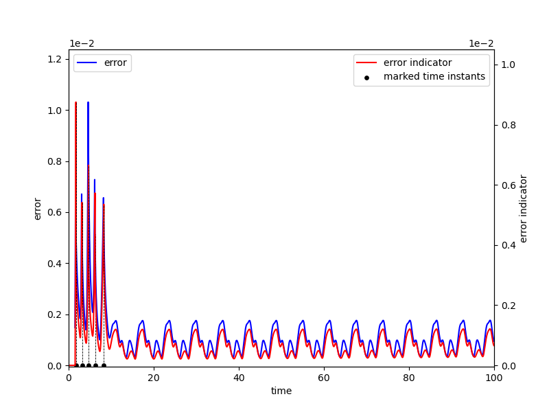
Figure 2: *

a).$\epsilon=0.5$.

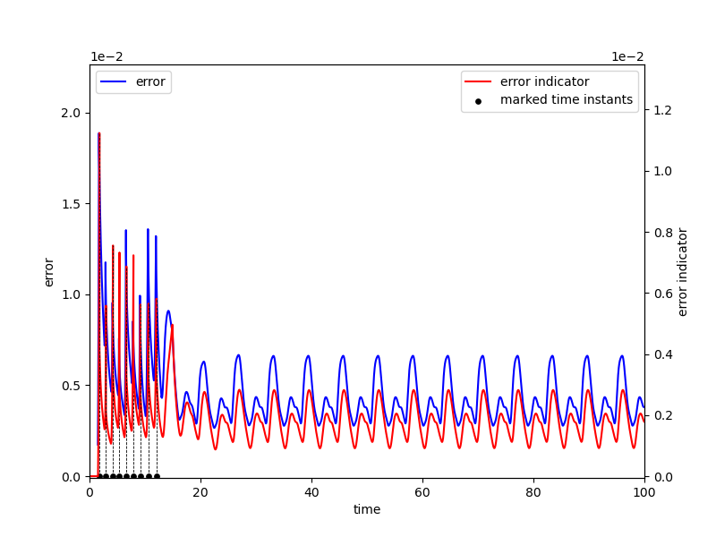
Figure 3: *

b).$\epsilon=0.1$.

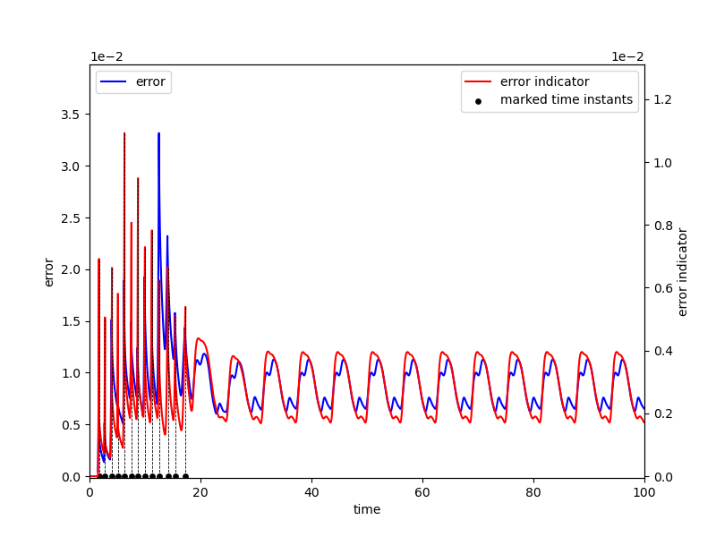
Figure 4: *

c).$\epsilon=0.05$.

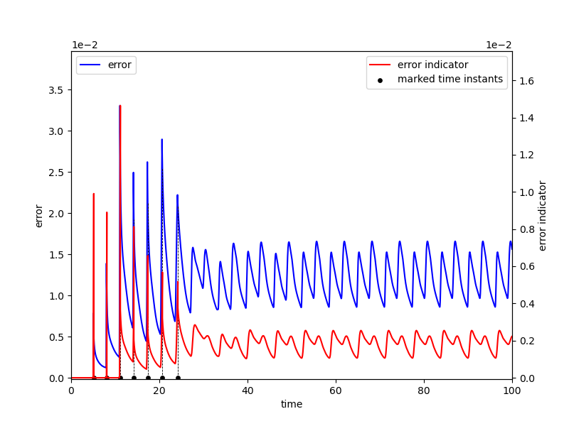
Figure 5: *

d).$\epsilon=0.01$.

Figure 6: The evolution curves of the error indicator and the error for solution of the Kolmogorov flow with $\epsilon=0.5,0.1,0.05,0.01$, respectively.

In Fig. 6, the y-axis in the left of each figure is the error which is defined by (20), while the y-axis in the right of each figure is the error indicator defined by (18), the black solid points denotes the time instances being marked which tell us when the POD modes need to be updated.

By carefully comparing the curves of the error indicator and the error in Fig 6, we can see that curves of the errors and error indicators are similar, although their magnitudes are somewhat different. Note that in our two-grid based adaptive POD method, the error indicator is used to indicate the change trend of the error, which then tells us the time instance when the POD modes should be updated. By comparing the curves of the error and the time instances being marked to be updated, we observe that the error indicator is efficient.

We then compare the numerical results obtained by our TG-APOD method, the residual-APOD method, and the standard POD method. The detailed results are listed in Table 1. The results obtained by standard finite element method are also provided as a reference.

As we have stated before, for our TG-APOD method, we choose the parameters $\gamma_{i}$ ($i=1,2,3$) and $\eta_{0}$ as: $\gamma_{1}=\gamma_{2}=0.999$, $\gamma_{3}=1.0-1.0\times 10^{-8}$, and $\eta_{0}=0.005$. While for the residual-APOD method, since people do not know how to set $\eta_{0}$ to obtained results with expected accuracy, they have to tune the parameter $\eta_{0}$. Therefore, to make the comparison reasonalble, we have tested the residual-APOD method by fixing $\gamma_{1}=\gamma_{2}=0.999$, $\gamma_{3}=1.0-1.0\times 10^{-8}$, but setting different values for $\eta_{0}$ to find out the best performance of the residual-APOD method.

In Table 1, ‘DOFs’ means the degree of freedom, ‘Time’ is the wall time for the simulation, ‘Average Error’ is the average of error for numerical solution in each time instance.

Table 1: The results of Kolmogorov flow with $\eta_{0}=0.005$ and different $\epsilon$ obtained by Standard-FEM, POD, Residual-APOD, and TG-APOD, respectively.

$\epsilon$	Methods	$\eta_{0}$	DOFs	Average Error	Time(s)
	Standard-FEM	–	4194304	–	13786.49
0.5	POD	–	13	0.193343	547.75
	Residual-APOD	$5\times 10^{-3}$	9	0.151803	5590.62
	Residual-APOD	$5\times 10^{-4}$	24	0.001166	6489.03
	TG-APOD	$5\times 10^{-3}$	24	0.001129	1511.63
	Standard-FEM	–	4194304	–	11950.82
0.1	POD	–	22	0.559466	535.47
	Residual-APOD	$5\times 10^{-3}$	28	0.167838	6241.83
	Residual-APOD	$8\times 10^{-4}$	44	0.012444	7099.24
	TG-APOD	$5\times 10^{-3}$	54	0.004524	2693.41
	Standard-FEM	–	4194304	–	11379.64
0.05	POD	–	16	0.805803	546.51
	Residual-APOD	$5\times 10^{-3}$	34	0.251224	6470.52
	Residual-APOD	$1\times 10^{-3}$	65	0.020072	7829.55
	TG-APOD	$5\times 10^{-3}$	83	0.008663	3959.62
	Standard-FEM	–	4194304	–	12955.44
0.01	POD	–	43	0.771091	1265.95
	Residual-APOD	$2\times 10^{-2}$	60	0.250940	7699.95
	Residual-APOD	$5\times 10^{-3}$	97	0.051444	9182.46
	TG-APOD	$5\times 10^{-3}$	138	0.010969	6299.70

We take a detailed look at Table 1. First, we can easily find that the degrees of freedom for all the POD type methods are indeed much smaller than those for the standard finite element method, which means that these POD type methods have good performance in dimensional reduction. Then, we can see from this example that the error of the numerical solution obtained by the standard POD method is too large, which makes the results meaningless. While both the residual based adaptive POD method and our two-grid based adaptive POD method can obtain numerical solution with higher accuracy, which validates the effectiveness of the adaptive POD methods. Next, let’s take a look at the results obtained by residual based adaptive POD method with diffferent $\eta_{0}$. We can see that as the decrease of the parameter $\eta_{0}$, the error of solutions obtained decreases while the cpu time cost increases. For different $\epsilon$, the gap between the error obtained by the residual based adaptive POD method and $\eta_{0}$ are different. While for our two-grid based adaptive POD method, the magnitude of the error is close to that of $\eta_{0}$, even for $\epsilon=0.01$. These coincides with what we have stated before. We also observe that as the decrease of $\epsilon$, the accuracy obtained by all the adaptive POD methods decreases, including our two-grid based POD method. We will pay more effort on the case with small $\epsilon$ in our future work. For the comparison of our method with the residual based adaptive POD method, we see that, by using the same parameters, the accuracy of results obtained by our method is much higher than those obtained by the residual based adaptive POD method, while the cpu time cost by our method is much less. Although by choosing proper $\eta_{0}$, the residual based adaptive POD method can obtain results as accurate as our method, the cpu time cost will be much more than that cost by our method. Anyway, taking both the accuracy and the cpu-time into account, we can see clearly that our method is more efficient than the residual based adaptive POD method.

To see more clearly, we compare the error of the numerical solutions obtained by the different methods in Fig. 11.

We should point out that among the different results obtained by residual-APOD with different $\eta_{0}$, we choose the best one to show in Fig.21.

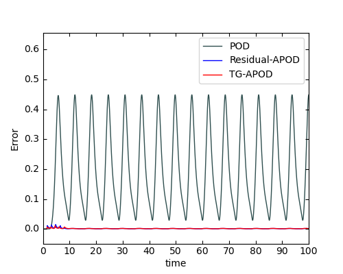
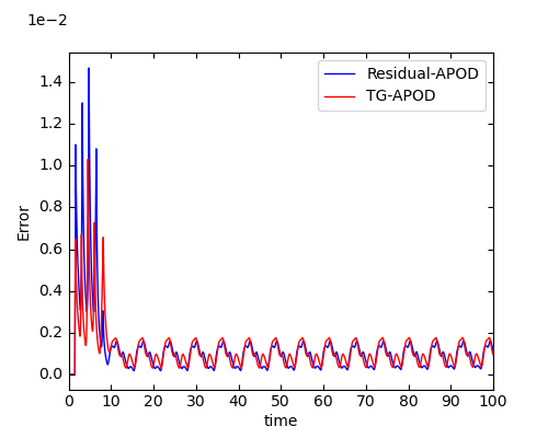
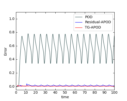
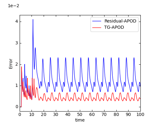
Figure 8: *

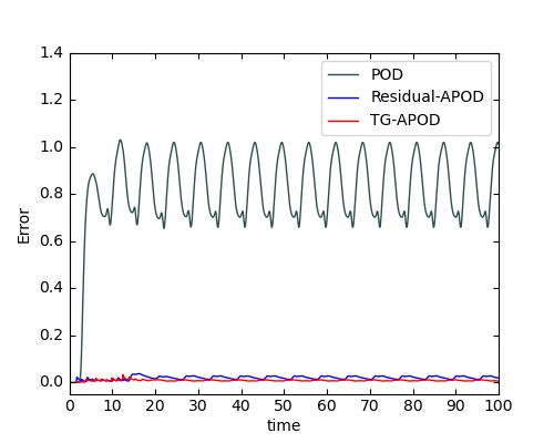
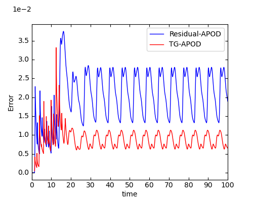
Figure 9: *

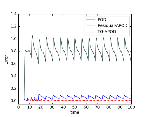
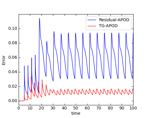
Figure 10: *

Figure 11: The error curves for solution of (21) with different $\epsilon$ obtained by the standard POD method, the residual based adaptive POD method, and the two-grid based adaptive POD method, respectively.

Figure 7: *

(a).$\epsilon=0.5$ (b).$\epsilon=0.1$ (c).$\epsilon=0.05$ (d).$\epsilon=0.01$

In Fig. 11, the x-axis is time, the y-axis is relative error of numerical solution. The results obtained by the standard POD method, the residual based adaptive POD algorithm, and our two-grid based adaptive POD algorithm are reported in lines with color darkslategray, blue, and red, respectively.

From the left figure of Fig. 11, we can see that the error curve obtained by the standard POD method is above both those obtained by the two adaptive POD methods, which means that the adaptive POD methods are more efficient than the standard POD method. From the right figure of Fig.2, we can see that our two-grid based adaptive POD method is more efficient than the residual based adaptive POD method.

4.2 Arnold-Beltrami-Childress (ABC) flow

We then consider the ABC flow. The ABC flow was introduced by Arnold, Beltrami, and Childress Kolmogorov-flow to study chaotic advection, enhanced transport and dynamo effect, see biferale1995eddy ; galanti1992linear ; wirth1995eddy ; xin2016periodic for the details.

We consider the following equation

$$\left\{\begin{aligned} &u_{t}-\epsilon\Delta u+\vec{B}(x,y,z,t)\cdot\nabla u=f(x,y,z,t),\quad(x,y,z)\in\Omega,t\in[0,T],\\ &u(x,y,z,0)=0,\\ &u(x+2\pi,y,z,t)=u(x,y+2\pi,z,t)=u(x,y,z+2\pi,t)=u(x,y,z,t),\\ \end{aligned}\right.$$ (22)

where

$$\vec{B}(x,y,z,t) = (\sin(z+\sin wt)+\cos(y+\sin wt),\sin(x+\sin wt)$$

$$+\cos(z+\sin wt),\sin(y+\sin wt)+\cos(x+\sin wt)),$$

$$f(x,y,z,t) = -\sin(z+\sin wt)-\cos(y+\sin wt),$$

$$\Omega=[0,2\pi ]^{3} ,T=100.$$

For this example, we also test $4$ different cases with $\epsilon=0.5,0.1$, $0.05$, and $0.01$, respectively. We divide the domain $[0,2\pi]^{3}$ into tetrahedrons to get the initial grid containing $6$ elements, then refine the initial mesh $22$ times uniformly using bisection to get the fine mesh. We set $w=1.0$, $\delta t=0.005$, and choose the finite element basis to be piecewise linear function. For the two cases with $\epsilon=0.5,0.1$, the parameters are chosen as $T_{0}=1.5,\delta T=1,\delta M=5$; for other cases with $\epsilon=0.05,0.01$, the parameters are chosen as $T_{0}=5,\delta T=4,\delta M=20$. In the two-grid based adaptive POD algorithm, we refine the initial mesh $16$ times uniformly using bisection to obtain the coarse mesh, and the time step of the coarse mesh is set to $0.09$. We use $36$ processors for the simulation.

We use the similar choice for parameters $\gamma_{i}$ ($i=1,2,3$) and $\eta_{0}$ as for the Kolmogorov flow. That is, for our two-grid based adaptive POD method, we choose them as $\gamma_{1}=\gamma_{2}=0.999$, $\gamma_{3}=1.0-1.0\times 10^{-8}$, and $\eta_{0}=0.005$, while for the residual-APOD method, we choose $\gamma_{1}=\gamma_{2}=0.999$, $\gamma_{3}=1.0-1.0\times 10^{-8}$, but setting different values for $\eta_{0}$ to find out the best performance of the residual-APOD method.

Similar to the Kolmogorov flow, we first use some numerical results to show the efficiency of our error indicator and the mark startegy. Fig 16 shows the evolution curves of the error indicator and the error, and the time instance being marked.

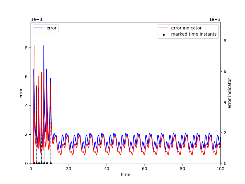
Figure 12: *

a).$\epsilon=0.5$.

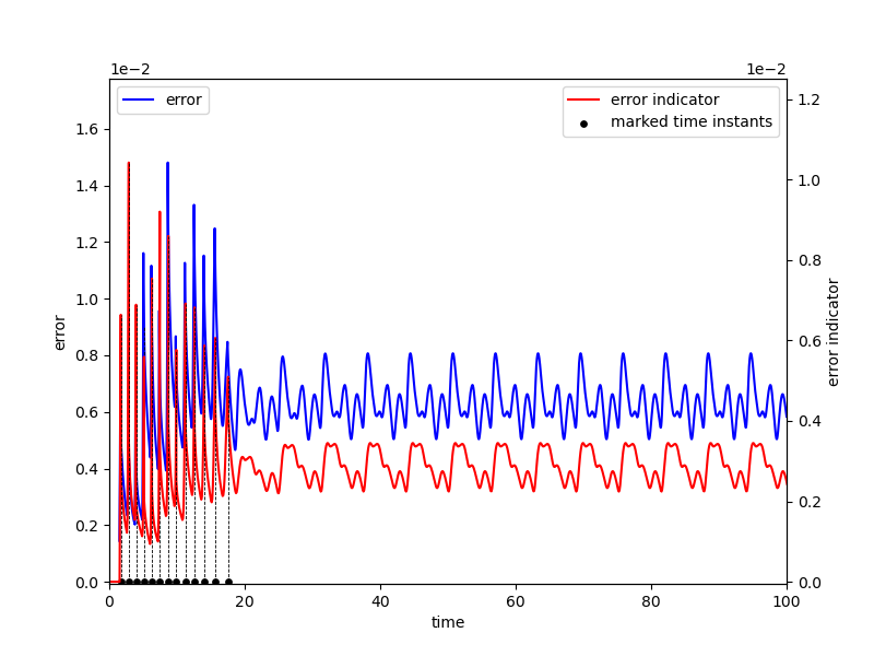
Figure 13: *

b).$\epsilon=0.1$.

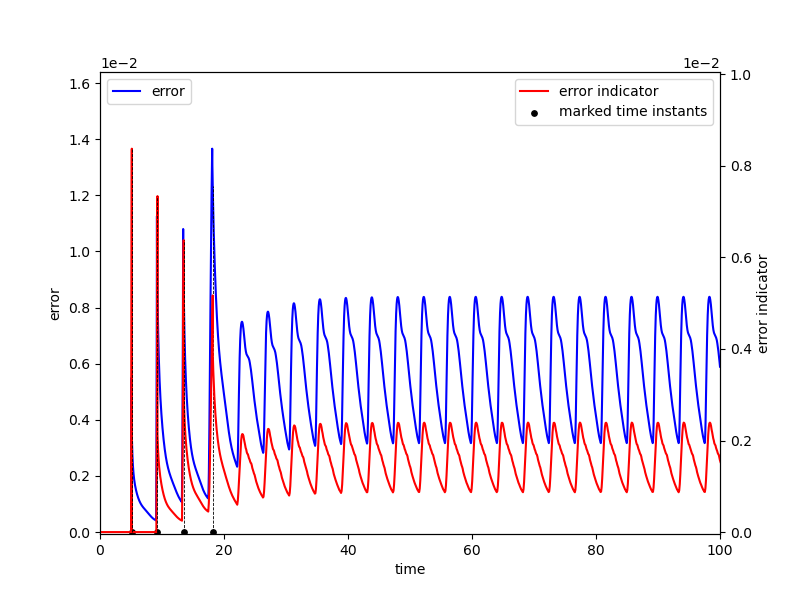
Figure 14: *

c).$\epsilon=0.05$.

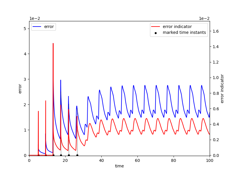
Figure 15: *

d).$\epsilon=0.01$.

Figure 16: The evolution curves of the error indicator and the error with $\epsilon=0.5,0.1,0.05,0.01$.

Similarly, by comparing the curves of the error indicator and the error, and the curve of the error and the time instance being marked to be updated in Fig. 16, we know that the error indicator is efficient.

We then compare the numerical results obtained by our two-grid based adaptive POD method, the residual-APOD method, the standard POD method. The detailed results are listed in Table 2. The results obtained by standard finite element method are also provided as a reference. The notation in Table 2 has the same meaning as in Table 1.

Table 2: The results of the ABC flow with different $\epsilon$ obtained by Standard-FEM, POD, Residual-APOD, and TG-APOD method, respectively.

$\epsilon$	Methods	$\eta_{0}$	DOFs	Average Error	Times (s)
0.5	Standard FEM	–	4194304	–	16690.55
	POD	–	12	0.303585	534.96
	Res-APOD	$5\times 10^{-3}$	9	0.191637	7749.15
	Res-APOD	$1\times 10^{-3}$	25	0.007640	8636.51
	TG-APOD	$5\times 10^{-3}$	33	0.001660	2240.67
0.1	FEM	–	4194304	–	15238.87
	POD	–	14	0.658382	536.73
	Res-APOD	$5\times 10^{-3}$	32	0.196853	9041.01
	Res-APOD	$1\times 10^{-3}$	57	0.024187	10213.65
	TG-APOD	$5\times 10^{-3}$	74	0.006207	4406.87
0.05	FEM	–	4194304	–	14439.24
	POD	–	42	0.504838	1485.62
	Res-APOD	$5\times 10^{-3}$	54	0.059658	10094.97
	Res-APOD	$1\times 10^{-3}$	67	0.014872	10734.27
	TG-APOD	$5\times 10^{-3}$	100	0.005077	5011.81
0.01	FEM	–	4194304	–	16074.96
	POD	–	61	0.676701	1878.01
	Res-APOD	$1\times 10^{-2}$	64	0.172755	10275.33
	Res-APOD	$5\times 10^{-3}$	140	0.042498	13322.86
	TG-APOD	$5\times 10^{-3}$	192	0.015851	10279.38

Similar to the first example, we can see from Table 2 that those POD type methods can indeed reduce the number of basis a lot. For this example, the accuracy for the approximation obtained by the standard POD method is so large that the results are meaningless. While both the residual based adaptive POD method and our two-grid based adaptive POD method can produce numerical solutions with high accuracy. For the two adaptive POD methods, our two-grid adaptive POD method can yield higher accuracy numerical solutions than the residual based adaptive POD method. When it comes to cpu time, our two-grid adaptive method takes less cpu time than the residual based adaptive POD method. These show that our two-grid adaptive POD method is more efficient.

Similarly, we show the error curves of the numerical solutions obtained by the different methods in Fig. 21.

In Fig. 21. the x-axis is time, the y-axis is the relative error of the POD approximations. The results obtained by the standard POD method, the residual based adaptive POD method, and our two-grid based adaptive POD method are reported in line with color darkslategray, blue, and red, respectively.

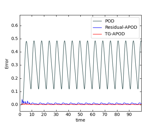
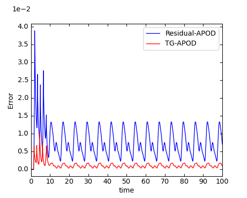
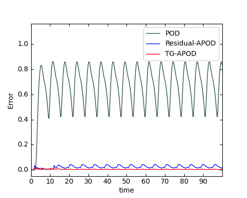
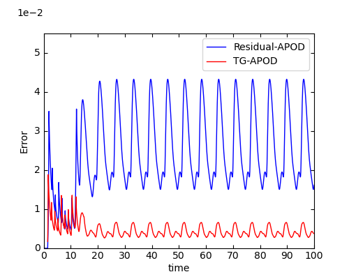
Figure 18: *

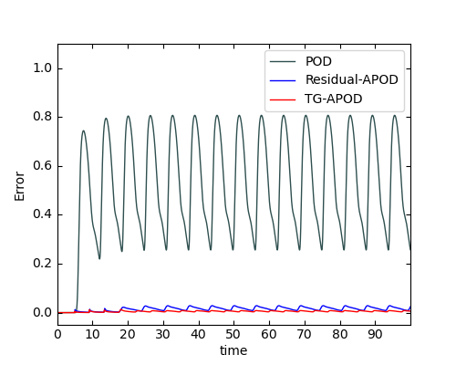
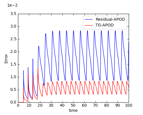
Figure 19: *

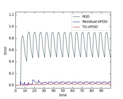
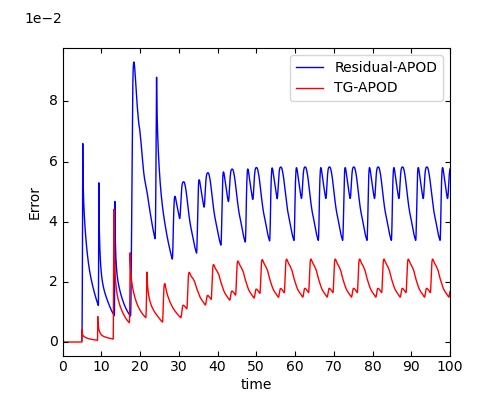
Figure 20: *

Figure 21: The evolution curves of error for solution of (22) with different $\epsilon$ obtained by the standard POD method, the residual based adaptive POD method, and the two-grid based adaptive POD method, respectively.

Figure 17: *

(a).$\epsilon=0.5$ (b).$\epsilon=0.1$ (c).$\epsilon=0.05$ (d).$\epsilon=0.01$

From Fig. 21, we can see more clearly that both the two-grid adaptive POD method and the residual based adaptive POD method behave much better than the standard POD method, and our two-grid based adaptive POD method behaves a little better than the residual based adaptive POD method.

We have done some more numerical experiments for setting different parameters $w$. The results for cases with $w=1.5,2,2.5$ are shown in Table 3.

Table 3: Results of the ABC flow with different $w$ and $\epsilon$ obtained by standard-FEM,POD, Residual-APOD and TG-APOD algorithm, respectively

$\epsilon$	$w$	Methods	$\eta_{0}$	DOFs	Average Error	Time (s)
0.5	1.5	FEM	–	4194304	–	16745.85
		POD	–	14	0.294394	561.23
		Res-APOD	$5\times 10^{-3}$	10	0.138573	7773.07
		Res-APOD	$5\times 10^{-4}$	30	0.003371	9017.68
		TG-APOD	$5\times 10^{-3}$	30	0.002611	2184.55
0.5	2.0	FEM	–	4194304	–	17258.89
		POD	–	15	0.270138	530.91
		Res-APOD	$5\times 10^{-3}$	6	0.336776	7581.42
		Res-APOD	$1\times 10^{-3}$	21	0.013750	8497.94
		TG-APOD	$5\times 10^{-3}$	31	0.001515	1927.63
0.5	2.5	FEM	–	4194304	–	17161.84
		POD	–	17	0.216109	602.85
		Res-APOD	$5\times 10^{-3}$	6	0.338068	7745.82
		Res-APOD	$5\times 10^{-4}$	21	0.008787	8440.45
		TG-APOD	$5\times 10^{-3}$	26	0.002678	1617.53
0.1	1.5	FEM	–	4194304	–	15232.78
		POD	–	15	0.729666	531.42
		Res-APOD	$5\times 10^{-3}$	32	0.148178	8576.58
		Res-APOD	$5\times 10^{-4}$	65	0.012987	10359.17
		TG-APOD	$5\times 10^{-3}$	78	0.006964	4238.26
0.1	2.0	FEM	–	4194304	–	15324.38
		POD	–	16	0.751065	536.24
		Res-APOD	$5\times 10^{-3}$	27	0.161848	8339.32
		Res-APOD	$5\times 10^{-4}$	57	0.018898	9790.15
		TG-APOD	$5\times 10^{-3}$	68	0.006915	3710.35
0.1	2.5	FEM	–	4194304	–	15104.35
		POD	–	18	0.657750	589.66
		Res-APOD	$5\times 10^{-3}$	21	0.222043	7886.83
		Res-APOD	$1\times 10^{-3}$	40	0.041986	9071.88
		TG-APOD	$5\times 10^{-3}$	75	0.005646	4212.24
0.05	1.5	FEM	–	4194304	–	14141.53
		POD	–	45	0.445832	1460.26
		Res-APOD	$5\times 10^{-3}$	42	0.148505	9410.69
		Res-APOD	$2\times 10^{-3}$	62	0.041819	10338.44
		TG-APOD	$5\times 10^{-3}$	98	0.004177	5361.94
0.05	2.0	FEM	–	4194304	–	14342.82
		POD	–	47	0.325020	1425.27
		Res-APOD	$5\times 10^{-3}$	44	0.088758	9303.73
		Res-APOD	$1\times 10^{-3}$	63	0.022060	10014.03
		TG-APOD	$5\times 10^{-3}$	83	0.004348	4299.98
0.05	2.5	FEM	–	4194304	–	14235.11
		POD	–	49	0.245578	1528.92
		Res-APOD	$5\times 10^{-3}$	46	0.057361	9220.55
		Res-APOD	$5\times 10^{-4}$	63	0.016595	10375.65
		TG-APOD	$5\times 10^{-3}$	84	0.007256	4313.27
0.01	1.5	FEM	–	4194304	–	16223.32
		POD	–	46	0.670506	1533.39
		Res-APOD	$2\times 10^{-2}$	95	0.155503	11154.77
		Res-APOD	$5\times 10^{-3}$	123	0.060578	12527.66
		TG-APOD	$5\times 10^{-3}$	187	0.016889	9337.59
0.01	2.0	FEM	–	4194304	–	16376.39
		POD	–	48	0.557215	1638.90
		Res-APOD	$8\times 10^{-3}$	97	0.122302	10954.07
		Res-APOD	$5\times 10^{-3}$	130	0.047402	12396.49
		TG-APOD	$5\times 10^{-3}$	194	0.010994	9371.19
0.01	2.5	FEM	–	4194303	–	16226.39
		POD	–	49	0.582593	1589.38
		Res-APOD	$1\times 10^{-2}$	64	0.172755	9645.38
		Res-APOD	$5\times 10^{-3}$	97	0.080639	11499.29
		TG-APOD	$5\times 10^{-3}$	188	0.015246	9427.31

From Table 3, we can obtain the same conclusion as those from Table 1 and Table 2, that is, adaptive POD methods outperform the POD method a lot, and our two-grid based adaptive method outperforms the residual based adaptive method.

5 Concluding remarks

In this paper, we proposed a two-grid based adaptive POD method to solve the time dependent partial differential equations. We apply our method to some typical 3D advection-diffusion equations, the Kolmogorov flow and the ABC flow. Numerical results show that our two-grid based adaptive POD method is more efficient than the residual based adaptive POD method, especially is much more efficient than the standard POD method. We should also point out that for problems with extreme sharp phase change, our method may behave not so well. Here, we simply use the relative error of the POD solution on the coarse spacial and temporal mesh to construct the error indicator. In our future work, we will consider other error indicator based on our two-grid approach or some other approach, and study other types of time dependent partial differential equations.

Appendix A A Numerical experiments for tuning parameters $\gamma_{i}(i=1,2,3)$

In this section, we do some numerical experiments for tuning the parameters $\gamma_{i}(i=1,2,3)$ to find out a good choice.

Since the parameters $\gamma_{1}$ and $\gamma_{2}$ are both for extracting POD modes from the snapshots obtained from the standard finite element approximation of the original dynamic system, we set them to be the same value, that is, $\gamma_{1}=\gamma_{2}$. We have tested the Kolmogorov flow with $\epsilon=0.05$ and $\epsilon=0.01$ respectively, and the ABC flow with $\epsilon=0.01$ by using the following different parameters:

• case 1: $\gamma_{1}=\gamma_{2}=1.0-1.0\times 10^{-8}$, set $\gamma_{3}$ to be $0.9,0.99,0.999,$ and $0.9999$ respectively.

• case 2: $\gamma_{3}=1.0-1.0\times 10^{-8}$, set $\gamma_{1}$ and $\gamma_{2}$ to be $0.9,0.99,0.999,$ and $0.9999$ respectively.

• case 3: $\gamma_{1}=\gamma_{2}=\gamma_{3}=1.0-1.0\times 10^{-2},1.0-1.0\times 10^{-4},1.0-1.0\times 10^{-6},1.0-1.0\times 10^{-8}$, respectively.

In our experiments, we choose $\eta_{0}=0.005$. The other parameters are same as stated in Section 4.

Kolmogorov flow with $\epsilon=0.01$

We first see the results for the Kolmogorov flow with $\epsilon=0.01$.

The results for case 1 are shown in Table 4. We can see that for fixing $\gamma_{1}$ and $\gamma_{2}$, the smaller $\gamma_{3}$, the more accurate the results, which means $\gamma_{3}$ close to $1$ may be a good choice. Then, we can see that when $\gamma_{1}$ and $\gamma_{2}$ are chosen to be too close to $1$, no matter how to choose the parameter $\gamma_{3}$, the cpu-time cost is too much. These results tell us that setting $\gamma_{1}$ and $\gamma_{2}$ too close to $1$ is not a good choice.

Table 4: Detailed information for results of the Kolmogorov flow with $\epsilon=0.01$ obtained by setting $\gamma_{1}=\gamma_{2}=1.0-1.0\times 10^{-8}$ and $\gamma_{3}=0.9,0.99,0.999,0.9999$, respectively.

	POD-updates	DOFs	Average Error	Times (s)
$\gamma_{3}=0.9$	30	66	0.059832	15770.89
$\gamma_{3}=0.99$	30	236	0.027262	31568.01
$\gamma_{3}=0.999$	22	339	0.018255	38263.16
$\gamma_{3}=0.9999$	6	222	0.043950	9501.85

The results for case 2 are shown in Table 5, from which we can see that for fixed $\gamma_{3}$, which is very close to $1$, setting $\gamma_{1}$ and $\gamma_{2}$ to be $0.999$ can obtain results with high accuracy. Taking into account the cpu time cost, $0.999$ is a better choice.

Table 5: Detailed information for results of the Kolmogorov flow with $\epsilon=0.01$ obtained by setting $\gamma_{3}=1.0-1.0\times 10^{-8}$ and $\gamma_{1}=\gamma_{2}=0.9,0.99,0.999,0.9999$, respectively.

	POD-updates	DOFs	Average Error	Times (s)
$\gamma_{1}=\gamma_{2}=0.9$	17	124	0.031398	7140.06
$\gamma_{1}=\gamma_{2}=0.99$	7	108	0.014088	4322.85
$\gamma_{1}=\gamma_{2}=0.999$	7	138	0.010969	6299.70
$\gamma_{1}=\gamma_{2}=0.9999$	7	185	0.015274	8457.13

The results for case 3 are shown in Table 6. We see that taking into account both the accuracy and the cpu time cost, these parameters are not as good as those for case 2.

Table 6: Detailed information for results of the Kolmogorov flow with $\epsilon=0.01$ obtained by setting $\gamma_{1}=\gamma_{2}=\gamma_{3}=\gamma=1.0-1.0\times 10^{-2},1.0-1.0\times 10^{-4},1.0-1.0\times 10^{-6},1.0-1.0\times 10^{-8}$ respectively.

	POD-updates	POD-DOFs	Average Error	Times (s)
$\gamma=1-10^{-2}$	31	55	0.013877	15354.34
$\gamma=1-10^{-4}$	7	182	0.012155	8351.72
$\gamma=1-10^{-6}$	6	204	0.024557	8826.03
$\gamma=1-10^{-8}$	6	223	0.043659	9585.60

Anyway, by comparing Table 4, Table 5, Table 6, we can see that the case of $\gamma_{1}=\gamma_{2}=0.999$, $\gamma_{3}=1.0-1.0\times 10^{-8}$ is the best choice among all these cases, if taking both the accuracy and the cpu-time cost into account.

the Kolmogorov flow with $\epsilon=0.05$

We then take a look at the results for the Kolmogorov flow with $\epsilon=0.05$, which are shown in Table7, Table 8, and Table 9.

Table 7: Detailed information for results of the Kolmogorov flow with $\epsilon=0.05$ obtained by setting $\gamma_{1}=\gamma_{2}=1.0-1.0\times 10^{-8}$ and $\gamma_{3}=0.9,0.99,0.999,0.9999$, respectively.

	POD-updates	DOFs	Average Error	Times (s)
$\gamma_{3}=0.9$	92	86	0.159828	16482.18
$\gamma_{3}=0.99$	92	473	0.076002	52158.13
$\gamma_{3}=0.999$	65	658	0.031944	86469.45
$\gamma_{3}=0.9999$	10	182	0.007093	7415.55

Table 8: Detailed information for results of the Kolmogorov flow with $\epsilon=0.05$ obtained by setting $\gamma_{3}=1.0-1.0\times 10^{-8}$ and $\gamma_{1}=\gamma_{2}=0.9,0.99,0.999,0.9999$, respectively.

	POD-updates	DOFs	Average Error	Times (s)
$\gamma_{1}=\gamma_{2}=0.9$	17	37	0.028841	3114.22
$\gamma_{1}=\gamma_{2}=0.99$	14	59	0.012810	3645.05
$\gamma_{1}=\gamma_{2}=0.999$	13	83	0.008663	3959.62
$\gamma_{1}=\gamma_{2}=0.9999$	12	109	0.007722	4690.68

Table 9: Detailed information for results of the Kolmogorov flow with $\epsilon=0.05$ obtained by setting $\gamma_{1}=\gamma_{2}=\gamma_{3}=\gamma=1.0-1.0\times 10^{-2},1.0-1.0\times 10^{-4},1.0-1.0\times 10^{-6},1.0-1.0\times 10^{-8}$ respectively.

	POD-updates	POD-DOFs	Average Error	Times (s)
$\gamma=1-10^{-2}$	92	49	0.023817	12711.97
$\gamma=1-10^{-4}$	13	104	0.006539	4726.16
$\gamma=1-10^{-6}$	11	152	0.006474	6421.31
$\gamma=1-10^{-8}$	10	188	0.007049	7739.79

By comparing Table 7, Table 8, Table 9, we can also see that the case of $\gamma_{1}=\gamma_{2}=0.999$, $\gamma_{3}=1.0-1.0\times 10^{-8}$ is the best choice among all these cases if taking both the accuracy and the cpu-time cost into account.

ABC flow with $\epsilon=0.01$

We have also done some numerical experiments for the ABC flow with $\epsilon=0.01$. For this example, the results obtained by setting different choice of the parameters $\gamma_{i}(i=1,2,3)$ are shown in Table 10, Table 11, and Table 12. From these results, we can obtain the same conclusion as those obtained from the Kolmogorov flow, that is, $\gamma_{1}=\gamma_{2}=0.999$, $\gamma_{3}=1.0-1.0\times 10^{-8}$ is the best choice among all these cases if taking into account both the accuracy and the cpu-time cost.

Table 10: Detailed information for results of the ABC flow with $\epsilon=0.01$ obtained by setting $\gamma_{1}=\gamma_{2}=1.0-1.0\times 10^{-8}$ and $\gamma_{3}=0.9,0.99,0.999,0.9999$, respectively.

	POD-updates	DOFs	Average Error	Times (s)
$\gamma_{3}=0.9$	22	78	0.078965	19831.24
$\gamma_{3}=0.99$	21	239	0.043133	37962.03
$\gamma_{3}=0.999$	19	393	0.015433	49428.57
$\gamma_{3}=0.9999$	7	318	0.043027	18551.14

Table 11: Detailed information for results of the ABC flow with $\epsilon=0.01$ obtained by setting $\gamma_{3}=1.0-1.0\times 10^{-8}$ and $\gamma_{1}=\gamma_{2}=0.9,0.99,0.999,0.9999$, respectively.

	POD-updates	DOFs	Average Error	Times (s)
$\gamma_{1}=\gamma_{2}=0.9$	14	134	0.037092	13922.37
$\gamma_{1}=\gamma_{2}=0.99$	7	146	0.011630	10635.61
$\gamma_{1}=\gamma_{2}=0.999$	6	192	0.015851	10279.38
$\gamma_{1}=\gamma_{2}=0.9999$	6	237	0.020604	12319.63

Table 12: Detailed information for results of the ABC flow with $\epsilon=0.01$ obtained by setting $\gamma_{1}=\gamma_{2}=\gamma_{3}=\gamma=1.0-1.0\times 10^{-2},1.0-1.0\times 10^{-4},1.0-1.0\times 10^{-6},1.0-1.0\times 10^{-8}$ respectively.

	POD-updates	POD-DOFs	Average Error	Times (s)
$\gamma=1-10^{-2}$	24	78	0.022985	19687.06
$\gamma=1-10^{-4}$	7	262	0.014736	14718.30
$\gamma=1-10^{-6}$	6	275	0.031665	14256.98
$\gamma=1-10^{-8}$	5	245	0.054979	11788.47

Appendix B B Numerical experiments for different coarse grid

Here, we use some numerical experiments to show how the degree of freedom for the coarse grid affects the accuracy and the cpu time cost when the fine grid is fixed. We hope it can provide some useful information about how to choose the coarse grid.

We take the Kolmogorov flow with $\epsilon=0.01$ as an example to show the behavior of our two-grid adaptive POD algorithm with different coarse mesh. In our experiments, we fix the fine mesh as what is shown in the manuscript, the other parameters are also set as the same as those used for obtaining results shown in Table 1. That is, we set $\gamma_{1}=\gamma_{2}=0.999$, $\gamma_{3}=1.0-1.0\times 10^{-8}$, and $\eta_{0}=0.005$. The detailed numerical results are listed in Table 13.

In Table 13, ‘N-Refine’ means the number of refinement used to obtain the mesh from the initial mesh, ‘Time step’ means the time step used for the coarse mesh, ‘DOFs-CoarseGrid’ means the degree of freedom corresponding to the coarse grid, ‘DOFs-POD’ means number of POD modes corresponding to the coarse grid, ‘POD-updates’ means the number of updation of the POD modes, ‘Average Error’ is computed by averaging the errors of numerical solution for each time instance, ‘Time-CoarseGrid’ is the wall time for the simulation on the coarse grid, ‘Total-Time’ is the wall time for all the simulation.

Table 13: The results of Kolmogorov flow with $\epsilon=0.01$ obtained by TG-APOD with different coarse mesh, respectively.

N-Refine	15	16	17	18	19
Time step	0.1	0.09	0.05	0.03	0.01
DOFs-CoarseGrid	32768	65536	163840	262144	524288
Time-CoarseGrid	17.47	34.03	133.46	882.47	1087.41
POD-updates	7	7	8	8	8
DOFs-POD	155	138	175	174	175
Average Error	0.011799	0.010969	0.006300	0.004592	0.003830
Total-Time(s)	7350.98	6299.70	9787.82	9312.94	9526.88

To see more clearly, we compare the error of numerical solutions obtained by TG-APOD with different coarse mesh in Fig 22.

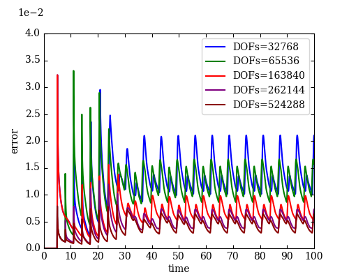
Figure 22: The change of error for the solution of Kolmogorov flow with $\epsilon=0.01$ obtained by TG-APOD with different coarse mesh.

From Table 13 and Fig. 22, we can see that as the degree of freedom for the coarse mesh increases, the average error will decrease, while the cpu time cost may increase. Therefore, there is a balance for the accuracy and the cpu time cost. For our case, taking into account the accuracy and the cpu time cost, we choose the coarse grid obtained by refine $16$ times from the initial mesh.

If we take a detailed look at Table 13, we will find that the cpu time cost is not only affected by the degree of freedom for the coarse grid. In fact, if the degree of freedom for the coarse mesh are not so large, the cpu time will be mainly determined by the number of POD modes updates (the process of basis update requires discretize the original equation with finite element basis for a period of time, which is expensive), which is mainly determined by the $\eta_{0}$. However, as the degree of freedom for the coarse mesh increases, the cpu time cost by calculating the error indicator on the coarse mesh also needs to be considered. Anyway, it is not easy to determine how large the coarse mesh is for the maximum efficiency.

References

- (1) Acary, V., Brogliato, B.: Implicit euler numerical scheme and chattering-free implementation of sliding mode systems. Systems & Control Letters. 59(5), 284–293 (2010)
- (2) Atwell, J.A., King, B.B.: Proper orthogonal decomposition for reduced basis feedback controllers for parabolic equations. Mathematical and Computer Modelling. 33(1-3), 1–19 (2001)
- (3) Bakker, M.: Simple groundwater flow models for seawater intrusion. Proceedings of SWIM16, Wolin Island, Poland. pp. 180–182 (2000)
- (4) Benner, P., Gugercin, S., Willcox, K.: A survey of projection-based model reduction methods for parametric dynamical systems. SIAM Review. 57(4), 483–531 (2015)
- (5) Bieterman, M., Babuška, I.: The finite element method for parabolic equations. Numerische Mathematik. 40(3), 373–406 (1982)
- (6) Biferale, L., Crisanti, A., Vergassola, M., Vulpiani, A.: Eddy diffusivities in scalar transport. Physics of Fluids. 7(11), 2725–2734 (1995)
- (7) Borggaard, J., Iliescu, T., Wang, Z.: Artificial viscosity proper orthogonal decomposition. Mathematical and Computer Modelling. 53(1-2), 269–279 (2011)
- (8) Boyaval, S., Le Bris, C., Lelievre, T., Maday, Y., Nguyen, N.C., Patera, A.T.: Reduced basis techniques for stochastic problems. Archives of Computational Methods in Engineering. 17(4), 435–454 (2010)
- (9) Brenner, S., Scott, R.: The mathematical theory of finite element methods. Springer, New York (2007)
- (10) Bueno-Orovio, A., Kay, D., Burrage, K.: Fourier spectral methods for fractional-in-space reaction-diffusion equations. BIT Numerical Mathematics. 54(4), 937–954 (2014)
- (11) Burkardt, J., Gunzburger, M., Lee, H.C.: POD and CVT-based reduced-order modeling of Navier–Stokes flows. Computer Methods in Applied Mechanics and Engineering. 196(1-3), 337–355 (2006)
- (12) Cannon, J.R.: The one-dimensional heat equation. Addison-Wesley, Mento Park,CA (1984)
- (13) Chen, H., Dai, X., Gong, X., He, L., Zhou, A.: Adaptive finite element approximations for Kohn–Sham models. Multiscale Modeling & Simulation. 12(4), 1828–1869 (2014)
- (14) Childress, S., Gilbert, A.D.: Stretch, Twist, Fold: the Fast Dynamo. Springer, Berlin (1995)
- (15) Chinesta, F., Huerta, A., Rozza, G., Willcox, K.: Model reduction methods. Encyclopedia of Computational Mechanics Second Edition. pp. 1–36 (2017)
- (16) Dai, X., Kuang, X., Liu, Z., Jack, X., Zhou, A.: An adaptive proper orthogonal decomposition galerkin method for time dependent problems. preprint (2017)
- (17) Dai, X., Xu, J., Zhou, A.: Convergence and optimal complexity of adaptive finite element eigenvalue computations. Numerische Mathematik. 110(3), 313–355 (2008)
- (18) Dai, X., Zhou, A.: Three-scale finite element discretizations for quantum eigenvalue problems. SIAM Journal on Numerical Analysis. 46(1), 295–324 (2008)
- (19) Feldmann, P., Freund, R.W.: Efficient linear circuit analysis by padé approximation via the lanczos process. IEEE Transactions on Computer-Aided Design of Integrated Circuits and Systems. 14(5), 639–649 (1995)
- (20) Forrester, A.I., Sóbester, A., Keane, A.J.: Multi-fidelity optimization via surrogate modelling. Proceedings of the Royal Society A: Mathematical, Physical and Engineering Sciences. 463(2088), 3251–3269 (2007)
- (21) Galanti, B., Sulem, P.L., Pouquet, A.: Linear and non-linear dynamos associated with abc flows. Geophysical & Astrophysical Fluid Dynamics. 66(1-4), 183–208 (1992)
- (22) Galloway, D.J., Proctor, M.R.: Numerical calculations of fast dynamos in smooth velocity fields with realistic diffusion. Nature. 356, 691–693 (1992)
- (23) Gräßle, C., Hinze, M.: POD reduced-order modeling for evolution equations utilizing arbitrary finite element discretizations. Advances in Computational Mathematics. 44(6), 1941–1978 (2018)
- (24) Gugercin, S., Antoulas, A.C.: A survey of model reduction by balanced truncation and some new results. International Journal of Control. 77(8), 748–766 (2004)
- (25) Hesthaven, J.S., Rozza, G., Stamm, B.: Certified reduced basis methods for parametrized partial differential equations, vol. 590. Springer (2016)
- (26) Ito, K., Ravindran, S.: A reduced-order method for simulation and control of fluid flows. Journal of Computational Physics. 143(2), 403–425 (1998)
- (27) Kosloff, D., Kosloff, R.: A fourier method solution for the time dependent schrödinger equation as a tool in molecular dynamics. Journal of Computational Physics. 52(1), 35–53 (1983)
- (28) Kunisch, K., Volkwein, S.: Galerkin proper orthogonal decomposition methods for parabolic problems. Numerische Mathematik. 90(1), 117–148 (2001)
- (29) Kunisch, K., Volkwein, S.: Optimal snapshot location for computing POD basis functions. ESAIM: Mathematical Modelling and Numerical Analysis. 44(3), 509–529 (2010)
- (30) LeVeque, R.J.: Finite difference methods for ordinary and partial differential equations: steady-state and time-dependent problems. SIAM,Philadelphia (2007)
- (31) Lumley, J.L.: The structure of inhomogeneous turbulent flows. Atmospheric Turbulence and Radio Wave Propagation. pp. 166–178 (1967)
- (32) Ly, H.V., Tran, H.T.: Modeling and control of physical processes using proper orthogonal decomposition. Mathematical and Computer Modelling. 33(1-3), 223–236 (2001)
- (33) Lyu, J., Xin, J., Yu, Y.: Computing residual diffusivity by adaptive basis learning via spectral method. Numerical Mathematics: Theory, Methods and Applications. 10(2), 351–372 (2017)
- (34) Maday, Y.: Reduced basis method for the rapid and reliable solution of partial differential equations. in Proceedings of International Conference of Mathematicians. pp. 1255–1270, European Mathematical Society, volume III (2006)
- (35) Maday, Y., Rønquist, E.M.: A reduced-basis element method. Journal of Scientific Computing. 17(1-4), 447–459 (2002)
- (36) Ng, L.W., Willcox, K.E.: Multifidelity approaches for optimization under uncertainty. International Journal for Numerical Methods in Engineering. 100(10), 746–772 (2014)
- (37) Obukhov, A.M.: Kolmogorov flow and laboratory simulation of it. Russian Mathematical Surveys. 38(4), 113–126 (1983)
- (38) Peherstorfer, B., Willcox, K.: Dynamic data-driven reduced-order models. Computer Methods in Applied Mechanics and Engineering. 291, 21–41 (2015)
- (39) Peherstorfer, B., Willcox, K., Gunzburger, M.: Survey of multifidelity methods in uncertainty propagation, inference, and optimization. SIAM Review. 60(3), 550–591 (2018)
- (40) PHG: http://lsec.cc.ac.cn/phg/
- (41) Pinnau, R.: Model reduction via proper orthogonal decomposition. In: Model Order Reduction: Theory, Research Aspects and Applications, pp. 95–109. Springer, Berlin, Heidelberg (2008)
- (42) Quarteroni, A., Rozza, G.: Reduced Order Methods for Modeling and Computational reduction, vol. 9. Springer,Berlin (2014)
- (43) Rapún, M.L., Terragni, F., Vega, J.M.: Adaptive pod-based low-dimensional modeling supported by residual estimates. International Journal for Numerical Methods in Engineering. 104(9), 844–868 (2015)
- (44) Rapún, M.L., Vega, J.M.: Reduced order models based on local pod plus galerkin projection. Journal of Computational Physics. 229(8), 3046–3063 (2010)
- (45) Shen, L., Xin, J., Zhou, A.: Finite element computation of KPP front speeds in 3d cellular and abc flows. Mathematical Modelling of Natural Phenomena. 8(3), 182–197 (2013)
- (46) Sirovich, L.: Turbulence and the dynamics of coherent structures. Part I: Coherent structures. Quarterly of Applied Mathematics. 45(3), 561–571 (1987)
- (47) Smith, G.D.: Numerical solution of partial differential equations: finite difference methods. Applied Mathematics and Computation,Oxford (1986)
- (48) Teckentrup, A.L., Jantsch, P., Webster, C.G., Gunzburger, M.: A multilevel stochastic collocation method for partial differential equations with random input data. SIAM/ASA Journal on Uncertainty Quantification. 3(1), 1046–1074 (2015)
- (49) Terragni, F., Vega, J.M.: Simulation of complex dynamics using pod’on the fly’and residual estimates. Dynamical Systems, Differential Equations and Applications AIMS Proceedings. pp. 1060–1069 (2015)
- (50) Thomée, V.: Galerkin finite element methods for parabolic problems, vol. 25. Springer-Verlag,Berlin (1984)
- (51) Tone, F., Wirosoetisno, D.: On the long-time stability of the implicit euler scheme for the two-dimensional navier–stokes equations. SIAM Journal on Numerical Analysis. 44(1), 29–40 (2006)
- (52) Volkwein, S.: Model reduction using proper orthogonal decomposition. Lecture Notes, Institute of Mathematics and Scientific Computing, University of Graz. 1025 (2011)
- (53) Wirth, A., Gama, S., Frisch, U.: Eddy viscosity of three-dimensional flow. Journal of Fluid Mechanics. 288, 249–264 (1995)
- (54) Xin, J., Yu, Y., Zlatos, A.: Periodic orbits of the abc flow with a= b= c= 1. SIAM Journal on Mathematical Analysis. 48(6), 4087–4093 (2016)
- (55) Xu, J., Zhou, A.: Local and parallel finite element algorithms based on two-grid discretizations. Mathematics of Computation. 69(231), 881–909 (2000)
- (56) Xu, J., Zhou, A.: A two-grid discretization scheme for eigenvalue problems. Mathematics of Computation. 70(233), 17–25 (2001)
- (57) Zu, P., Chen, L., Xin, J.: A computational study of residual kpp front speeds in time-periodic cellular flows in the small diffusion limit. Physica D: Nonlinear Phenomena. 311, 37–44 (2015)