The NN-Stacking: Feature weighted linear stacking through neural networks

Abstract

Stacking methods improve the prediction performance of regression models. A simple way to stack base regressions estimators is by combining them linearly, as done by Breiman [1]. Even though this approach is useful from an interpretative perspective, it often does not lead to high predictive power. We propose the NN-Stacking method (NNS), which generalizes Breiman’s method by allowing the linear parameters to vary with input features. This improvement enables NNS to take advantage of the fact that distinct base models often perform better at different regions of the feature space. Our method uses neural networks to estimate the stacking coefficients. We show that while our approach keeps the interpretative features of Breiman’s method at a local level, it leads to better predictive power, especially in datasets with large sample sizes.

1 Introduction

The standard procedures for model selection in prediction problems is cross-validation and data splitting. However, such an approach is known to be sub-optimal [2, 3, 4]. The reason is that one might achieve more accurate predictions by combining different regression estimators rather then by selecting the best one. Stacking methods [5] are a way of overcoming such a drawback from standard model selection.

A well known stacking method was introduced by Breiman [1]. This approach consists in taking a linear combination of base regression estimators. That is, the stacked regression has the shape $\sum_{i=1}^{k}\theta_{i}g_{i}({\mathbf{x}})$, where $g_{i}$’s are the individual regression estimators (such as random forests, linear regression or support vector regression), $\theta_{i}$ are weights that are estimated from data and ${\mathbf{x}}$ represents the features.

Even though this linear stacking method leads to combined estimators that are easy to interpret, it may be sub-optimal in cases where models have different local accuracy, i.e., situations where the performance of these estimators vary over the feature space. Example 1.1 illustrates this situation.

Example 1.1.

Consider predicting $Y$ based on a single feature, $x$, using the data in Figure 1. We fit two least squares estimators: $g_{1}({\mathbf{x}})=\theta_{01}+\theta_{11}x$ and $g_{2}({\mathbf{x}})=\theta_{02}+\theta_{12}x^{2}$. None of the models is uniformly better; for example, the linear fit has better performance when $x\leq 5$, but the quadratic fit yields better performance for $x\in(-2.5,2.5)$. One may take this into account when creating the stacked estimator by assigning different weights for each regression according to $x$: while one can assign a larger weight to the linear fit on the regime $x\leq 5$, a lower weight should be assigned to it if $x\in(-2.5,2.5)$.

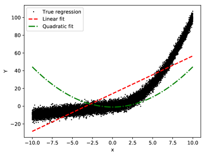
Figure 1: Regressions comparison. While for some regions of $x$ the linear fit outperforms the quadratic fit, in other regions the opposite happens.

It is well known that different regression methods may perform better on different regions of the feature space. For instance, because local estimators do not suffer from boundary effects, they achieve good performance closer to the edges of the feature space [6]. Random forests, on the other hand, implicitly perform feature selection, and thus may have better performance in regions where some features are not relevant [7].

In this work we improve Breiman’s approach so that it can take local accuracy into account. That is, we develop a meta-learner that is able to learn which models have higher importance on each region of the feature space. We achieve this goal by allowing each parameter $\theta_{i}$ to vary as a function of the features ${\mathbf{x}}$. In this way, the meta-learner can adapt to each region of the feature space, which yields higher predictive power. Our approach keeps the local interpretability of the linear stacking model.

The remaining of the work is organized as follows. Section 2 introduces the notation used in the paper, as well as our method. Section 3 shows details on its implementation. Section 4 shows applications of our method to a variety of datasets to evaluate its performance. Section 5 concludes the paper.

2 Notation and Motivation

The stacking method proposed by Breiman [1] is a linear combination of $k$ regression functions for a label $Y\in\mathbb{R}$. More precisely, let $g_{\mathbf{x}}=(g_{1}({\mathbf{x}}),g_{2}({\mathbf{x}}),\ldots,g_{k}({\mathbf{x}}))^{\prime}$ be a vector of regression estimators, that is, $g_{i}({\mathbf{x}})$ is an estimate of ${\textbf{E}}[Y|{\mathbf{x}}],\forall\,i=1,2,\ldots,k$. The linear stacked regression is defined as

$$G_{\theta}({\mathbf{x}}):=\sum_{i=1}^{k}\theta_{i}g_{i}({\mathbf{x}})=\theta^{\prime}g_{\mathbf{x}}$$ (2.1)

where $\theta=(\theta_{1},\theta_{2},\ldots,\theta_{k})^{\prime}$ are meta-parameters. One way to estimate the meta-parameters using data $({\mathbf{x}}_{1},y_{1}),\ldots,({\mathbf{x}}_{n},y_{n})$ is through the least squares method, computed using a leave-one-out setup:

$$\arg\min_{\theta}\sum_{i=1}^{n}(y_{i}-G^{(-i)}_{\theta}({\mathbf{x}}_{i}))^{2}=\arg\min_{\theta}\sum_{i=1}^{n}(y_{i}-\theta^{\prime}g_{{\mathbf{x}}_{i}}^{(-i)})^{2},$$ (2.2)

where $g_{j}^{(-i)}({\mathbf{x}}_{i})$ is the prediction for ${\mathbf{x}}_{i}$ made by the $j$-th regression fitted without the $i$-th instance. Note that it is important to use this hold-out approach because if the base regression functions $g_{1}({\mathbf{x}}),g_{2}({\mathbf{x}}),\ldots,g_{k}({\mathbf{x}})$ are constructed using the same data as $\theta_{1},\ldots,\theta_{k}$, this can cause $G_{\theta}({\mathbf{x}})$ to over-fit the training data.

In order for the stacked estimator to be easier to interpret, Breiman [1] also requires $\theta_{i}$’s to be weights, that is $\theta_{i}\geq 0\,\forall\,i=1,2,\ldots,k$ and that $\sum_{i=1}^{k}\theta_{i}=1$.

Even though Breiman’s solution works on a variety of settings, it does not take into account that each regression method may perform better in distinct regions of the feature space. In order to overcome this limitation, we propose the Neural Network Stacking (NNS) which generalizes Breiman’s approach by allowing $\theta$ on Equation 2.1 to vary with ${\mathbf{x}}$. That is, our meta-learner has the shape

$$G_{\theta}({\mathbf{x}}):=\sum_{i=1}^{k}\theta_{i}({\mathbf{x}})g_{i}({\mathbf{x}})=\theta_{x}^{\prime}g_{\mathbf{x}},$$ (2.3)

where $\theta_{x}:=(\theta_{1}({\mathbf{x}}),\theta_{2}({\mathbf{x}}),\ldots,\theta_{k}({\mathbf{x}}))^{\prime}$. In other words, the NNS is a local linear meta-learner. Example 2.1 shows that NNS can substantially decrease the prediction error of Breiman’s approach.

Example 2.1.

We fit both Breiman’s linear meta-learner and our NNS local linear meta-learner to the models fitted in Example 1.1. Figure 2 shows that Breiman’s meta-learner is not able to fit the true regression satisfactorily because both estimators have poor performance on specific regions of the data. On the other hand, feature-varying weights yield a better fit.

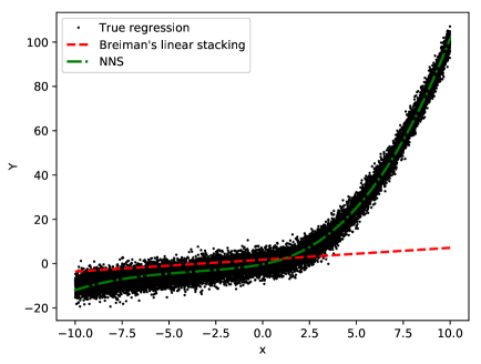
Figure 2: Meta-learners fits for Example 1.1. While Breiman’s meta-learner is not able to fit the true regression satisfactorily, feature varying weights yield better fit.

3 Methodology

Our goal is to find $\theta_{\mathbf{x}}=(\theta_{1}({\mathbf{x}}),\ldots,\theta_{k}({\mathbf{x}}))^{\prime}$, $\theta_{i}:\mathcal{X}\longrightarrow\mathbb{R}$, that minimizes the mean squared risk,

$$R(G_{\theta})={\textbf{E}}\left[\left(Y-G_{\theta}({\mathbf{X}})\right)^{2}\right],$$

where $G_{\theta}({\mathbf{x}})$ is defined as in Equation in 2.3.

We estimate $\theta_{\mathbf{x}}$ via an artificial neural network. This network takes ${\mathbf{x}}$ as input and produces an output $\theta_{\mathbf{x}}$, which is then used to obtain $G_{\theta}({\mathbf{x}})$. To estimate the weights of the networks, we introduce an appropriate loss function that captures the goal of having a small $R(G_{\theta})$. This is done by using the loss function

$$\frac{1}{n}\sum_{k=1}^{n}(G_{\theta}({\mathbf{x}}_{k})-y_{k})^{2}.$$

Notice that the base regression estimators are used only when evaluating the loss function; they are not the inputs of the network. With this approach, we allow each $\theta_{i}({\mathbf{x}})$ to be a complex function of the data. We call this method Unconstrained Neural Network Stacking (UNNS). Figure 3 illustrates a UNNS that stacks 2 base estimators in a regression problem with four features.

Figure 3: Example of a UNNS neural network.

In addition to the linear stacking, this approach allows the user to easily take advantage of the neural network architecture by directly adding a network output node, $\phi({\mathbf{x}})$, to the stacking. That is, we also consider a variation of UNNS which takes the shape

$$G^{\prime}_{\theta}({\mathbf{x}})=\theta^{\prime}_{\mathbf{x}}g_{\mathbf{x}}+\phi({\mathbf{x}}).$$

This has some similarity to adding a single neural network estimator to the stacking. However, we use the same architecture to create the additional term, mitigating computation time. Algorithm 1 shows how this method is implemented. In order to avoid over-fitting, $\theta_{i}$’s and $g_{i}$’s are estimated using different folds of the training set.

Algorithm 1 UNNS

Input: Estimation algorithms $g=(g_{1},g_{2},\ldots,g_{k})^{\prime}$, a dataset $D=(X,Y)$ with $n$ instances (rows), a neural network $N$, features to predict $X^{(p)}$, the amount of folds $F$.
Output: Predicted values $y^{(p)}$.

1:Let $I=\{I_{o}:o\in\{1,2,...,F\}\}$ be a random F-fold partition of the dataset instances, let $I^{(X)}$ refer to a partition of features and $I^{(Y)}$ refer to a partition of the response variable, both being partitioned on the same indices (i.e.: $I_{o}(i)=(I_{o}^{(X)}(i),I_{o}^{(Y)}(i))$ for every $o\in\{1,2,...,F\}\}$ and every $i\in\{1,2,...,n\}\}$), with the partition of indices $\{1,2,...,n\}$ represented by $I^{(l)}$.

2:Let $P$ be a $(n,k)$ matrix.

3:For $o\in\{1,2,...,F\}$ and $j\in\{1,2,...,k\}$, fit $g_{j}$ to $D\backslash I_{o}$, then use the fitted model to predict $I^{(X)}_{o}$ and store these predicted values on $P$ (in column $j$ and lines corresponding to $I_{o}^{(l)})$).

4:Let $\{g_{1}^{(f)},g_{2}^{(f)},...,g_{k}^{(f)}\}$ be the models $g$ fitted using the whole dataset $D$.

5:Train the neural network $N$ with each input instance $i$ given by a row of $X$; with $\theta(X_{i})=(\theta_{1}(X_{i}),\theta_{2}(X_{i}),...,\theta_{k}(X_{i}))$ and a scalar $\phi(X_{i})$ as outputs; and with loss function given by $(\sum_{j=1}^{k}\theta_{j}(X_{i})P_{ij}+\phi(X_{i})-y_{i})^{2}$ (note: the additional scalar $\phi$ is optional, i.e.: it can be set to zero).

6:For each instance $i$ of $X^{(p)}$, the corresponding predicted value $Y^{(p)}_{i}$ is then given by $\sum_{j=1}^{k}\theta_{j}(X^{(p)}_{i})g_{j}^{(f)}(X^{(p)}_{i})+\phi(X^{(p)}_{i})$ where $\theta(X^{(p)}_{i})$ and $\phi(X^{(p)}_{i})$ are outputs of the neural network (i.e.: $N(X^{(p)}_{i})$).

In order to achieve an interpretable stacked solution, we follow Breiman’s suggestion and consider a second approach to estimate $\theta_{i}$’s which consists in minimizing $R(G_{\theta})$ under the constrain that $\theta_{i}$’s are weights, that is, $\theta_{i}({\mathbf{x}})\geq 0$ and $\sum_{i=1}^{k}\theta_{i}({\mathbf{x}})=1$. Unfortunately, it is challenging to directly impose this restriction to the solution of the neural network. Instead, we use a different parametrization of the problem, which is motivated by Theorem 3.1.

Theorem 3.1.

The solution of

$$\arg\min_{\theta_{x}}R(G_{\theta})$$

under the constrain that $\theta_{i}({\mathbf{x}})\geq 0$ and $\sum_{i=1}^{k}\theta_{i}({\mathbf{x}})=1$ is given by

$$\theta_{\mathbf{x}}=\frac{\mathbb{M}^{-1}_{\mathbf{x}}\mathbf{e}}{\mathbf{e}^{\prime}\mathbb{M}^{-1}_{\mathbf{x}}\mathbf{e}},$$ (3.1)

where $\mathbf{e}$ is a $k$-dimensional vector of ones and

$$\mathbb{M}_{\mathbf{x}} =[{\textbf{E}}\left[(Y-g_{i}({\mathbf{x}}))(Y-g_{j}({\mathbf{x}}))\right|{\mathbf{X}}={\mathbf{x}}]_{ij}]$$

$$={\textbf{E}}[Y^{2}|{\mathbf{x}}]-{\textbf{E}}[Y|{\mathbf{x}}](g_{i}({\mathbf{x}})-g_{j}({\mathbf{x}})))+g_{i}({\mathbf{x}})g_{j}({\mathbf{x}}).$$

with $(i,j)\in\{1,...,k\}^{2}$.

Theorem 3.1 shows that, under the given constrains, $\theta({\mathbf{x}})$ is uniquely defined by $\mathbb{M}^{-1}_{\mathbf{x}}$. Now, because $\mathbb{M}_{\mathbf{x}}$ is a covariance matrix, then $\mathbb{M}^{-1}_{\mathbf{x}}$ is positive definite, and thus Cholesky decomposition can be applied to it. It follows that $\mathbb{M}^{-1}_{\mathbf{x}}=L_{\mathbf{x}}L_{\mathbf{x}}^{\prime}$, where $L_{\mathbf{x}}$ is a lower triangular matrix. This suggests that we estimate $\theta_{\mathbf{x}}$ by first estimating $L_{\mathbf{x}}$ and then plugging the estimate back into Equation 3.1. That is, in order to obtain a good estimator under the above mentioned restrictions, the output of the network is set to be $L_{\mathbf{x}}$ rather than the weights themselves. We name this method Constrained Neural Network Stacking (CNNS). Figure 4 illustrates a CNNS that stacks 2 base regressors (that is, $L_{\mathbf{x}}=[l_{ij}]$ is a $2x2$ triangular matrix) in a 4 feature regression problem.

Figure 4: Example of the CNNS neural network.

Algorithm 2 shows the implementation of this method. As with UNNS, we also explore a variation which adds an extra network output $\phi({\mathbf{x}})$ to $G_{\theta}$.

Algorithm 2 CNNS

Input: Estimation algorithms $g=(g_{1},g_{2},\ldots,g_{k})^{\prime}$, a dataset $D=(X,Y)$ with $n$ instances (rows), a neural network $N$, features to predict $X^{(p)}$, the amount of folds $F$.
Output: Predicted values $y^{(p)}$.

1:Follow steps 1 to 4 from algorithm 1.

2:Train the neural network $N$ with each input instance $i$ given by a row of $X$; with a lower triangular matrix $L_{X_{i}}$ and a scalar $\phi(X_{i})$ as outputs; and with loss function given by $(\sum_{j=1}^{k}\theta_{j}(X_{i})P_{ij}+\phi(X_{i})-y_{i})^{2}$, where $\mathbb{M}^{-1}=L_{X_{i}}L_{X_{i}}^{\prime}$ ; $\theta(X_{i})=\frac{\mathbb{M}^{-1}_{\mathbf{x}}\mathbf{e}}{\mathbf{e}^{\prime}\mathbb{M}^{-1}_{\mathbf{x}}\mathbf{e}}$ and $\mathbf{e}$ is a $k$-dimensional vector of ones (note: the additional scalar $\phi$ is optional, i.e.: it can be set to zero).

3:The predicted value $Y^{(p)}$ is calculated analogously to Algorithm 1.

Figure 5 illustrates the full training process. For simplicity, the neural network early stopping patience criterion is set to a single epoch and the additional parameter $\phi_{\mathbf{x}}$ is not used.

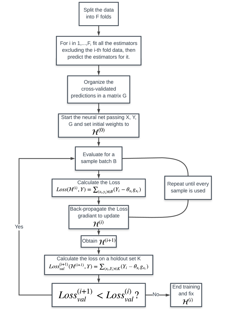
Figure 5: Full NN-Stacking training process.

3.1 Comparison with standard stacking methods

Most stacking methods create a meta-regression model by applying a regression method directly on the outputs of individual predictions. In particular, a meta-regression method can be a neural network. Such procedure differs from NN-Stacking by the shape of both the input and of the output of the network. While standard stacking uses base regression estimates ($g_{x}$) as input and $Y$ as output, NN-Stacking uses the features as input and either the weights $\theta_{x}$ (for UNSS) or $L_{\mathbf{x}}$ (for CNSS) as outputs. The base regression estimates are used only on the loss function. Thus, the NN-Stacking method leads to more interpretable models. Section 4 compares these methods in terms of their predictive power. We also point out that our approach has some similarity to Sill et al. [4], which allows each $\theta_{i}$ to depend on meta-features computed from ${\mathbf{x}}$ using a specific parametric form. Neural networks, on the other hand, provide a richer family of functions to model such dependencies (in fact, they are universal approximators; Csáji [8]).

3.2 Selecting base regressors

Consider the extreme case where $g_{i}({\mathbf{x}})=g_{j}({\mathbf{x}})\,\forall\,{\mathbf{x}}\in\mathcal{X}$ for some $i\neq j$, that is, the case in which two base regressors generate the same prediction over all feature space. Now, suppose that one fits a NNS (either CNNS or UNNS) for this case. Then $\theta_{i}g_{i}({\mathbf{x}})+\theta_{j}g_{j}({\mathbf{x}})=(\theta_{i}+\theta_{j})g_{i}({\mathbf{x}}).$ Thus, one of the regressions can be dropped from the stacking with no loss in predictive power.

In practice, our experiments (Section 4) show that regression estimators that have strongly correlated results do not contribute to the meta-learner. This suggests that one should choose base regressors with considerably distinct nature.

3.3 Implementation details

A Python package that implements the methods proposed in this paper is available at github.com/randommm/nnstacking. The scripts for the experiments in Section 4 are availiable at github.com/vcoscrato/NNStacking. We work with the following specifications for the artificial neural networks:

• Optimizer: we use the Adam algorithm [9] and decrease its learning rate after the validation loss stops improving for a user-defined number of epochs.

• Initialization: we use the Xavier Gaussian method proposed by Glorot and Bengio [10] to sample the initial parameters of the neural network.

• Layer activation and regularization: we use ELU [11] as the activation function, and do not use regularization.

• Normalization: we use batch normalization [12] to speed-up the training process.

• Stopping criterion: in order to address the risk of having strong over-fit on the neural networks, we worked with a 90%/10% split early stopping for small datasets and a higher split factor for larger datasets (increasing the proportion of training instances) and a patience of 10 epochs without improvement on the validation set.

• Dropout: We use dropout (with a rate of 50%) to address the problem of over-fitting [13].

• Software: we use PyTorch [14].

• Architecture: as default values we use a 3 layer depth network with hidden layer size set to 100; these values have been experimentally found to be suitable in our experiments (Section 4).

4 Experiments

We compare stacking methods for the following UCI datasets:

• The GPU kernel performance dataset (241600 instances, 13 features) [15],

• The music year prediction dataset [16] (515345 instances and 90 features),

• The blog feedback dataset [17] (60021 instances, 280 features),

• The superconductivity dataset [18] (21263 instances, 80 features).

First, we fit the following regression estimators (that will be stacked):

• Three linear models: with L1, L2, and no penalization [19],

• Two tree based models: bagging and random forests [19],

• A gradient boosting method (GBR) [20].

The tuning parameters of these estimators are chosen by cross-validation using scikit-learn [21].

Using these base estimators, we then fit four variations of NNS (both CNNS and UNNS with and without the additional $\phi_{x}$) using the following specifications:

• Tuning: three different architectures were tested for each neural network approach. The layer size was fixed at 100 and the number of hidden layers were set to 1, 3, and 10. We choose the architecture with the lowest validation mean-squared error.

• Train/validation/test split: for all datasets, we use 75% of the instances to fit the models, among which 10% are used for performing early stop. The remaining 25% of the instances are used as a test set to compare the performance of the various models. The train/test split is performed at random. The cross-validated predictions (the matrix $P$ denoted on Algorithm 1) are obtained using a 10-fold cross-validation on the training data (i.e., $F=10$).

• Total fitting time: we compute the total fitting time (in seconds; including the time for cross-validating the network architecture) of each method on two cores of an AMD Ryzen 7 1800X processor running at 3.6Gz.

We compare our methods with Breiman’s linear stacking and the usual neural net stacking model described in Section 3.1. In addition to these, we also include a comparison with a direct neural network that has ${\mathbf{x}}$ as its input and $Y$ as its output.

The comparisons are made by evaluating the mean squared error (MSE, $n^{-1}\sum_{i=1}^{n}(y_{i}-g({\mathbf{x}}_{i}))^{2}$) and the mean absolute error (MAE, $n^{-1}\sum_{i=1}^{n}|y_{i}-g({\mathbf{x}}_{i})|$) of each model $g$ on a test set. We also compute the standard error for each of these metrics, which enables one to compute confidence intervals for the errors of each method.

4.1 GPU kernel performance dataset

Table 1 shows the results that were obtained for the GPU kernel performance dataset. Our UNNS methods outperforms both Breiman’s stacking and the usual meta-regression stacking approaches in terms of MSE. Moreover, the UNNS model is also the best one in terms of MAE, even though the gap between the models is lower in this case. Our stacking methods also perform better than all base estimators. This suggests that each base model performs better on a distinct region of the feature space.

Figure 6 shows a boxplot with the distribution of the fitted $\theta_{i}$’s for UNNS. Many fitted values fall out of the range $[0,1]$, which explains why UNNS gives better results than Breiman’s and CNNS (which have the restriction that $\theta_{i}$’s must be proper weights).

Table 2 shows the correlation between the prediction errors for base estimators. The linear estimators had an almost perfect pairwise correlation, which indicates that removing up to 2 of them from the stacking would not affect predictions. Indeed, after refitting UNNS without using ridge regression and lasso, we obtain exactly the same results. We also refit the best UNNS removing all of the linear estimators to check if poor performing estimators are making stacking results worse. In this setting, we obtain an MSE of $11074.13(\pm 227.57)$, and a MAE of $45.76(\pm 0.39)$. Note that although the point estimates of the errors are lower than those obtained in Table 1, the confidence intervals have an intersection, which leads to the conclusion that the poor performance of linear estimators is not damaging the stacked estimator.

Type Model MSE MAE Total fit time Stacked estimators UNNS + $\phi_{x}$ (3 layers) 11400.43 ($\pm$ 250.03) 45.91 ($\pm$ 0.39) 3604 CNNS + $\phi_{x}$ (3 layers) 19371.98 ($\pm$ 429.96) 53.09 ($\pm$ 0.52) 3531 UNNS (3 layers) 11335.85 ($\pm$ 241.94) 45.85 ($\pm$ 0.39) 3540 CNNS (3 layers) 18748.66 ($\pm$ 424.5) 51.65 ($\pm$ 0.52) 3387 Breiman’s stacking 30829.11 ($\pm$ 717.13) 62.41 ($\pm$ 0.67) 63 Meta-regression neural net (10 layers) 24186.4 ($\pm$ 545.52) 58.79 ($\pm$ 0.59) 85 Direct estimator Direct neural net (10 layers) 14595.98 ($\pm$ 307.11) 52.3 ($\pm$ 0.44) 380 Base estimators Least squares 79999.09 ($\pm$ 1504.75) 176.41 ($\pm$ 0.9) - Lasso 80091.85 ($\pm$ 1526.05) 175.5 ($\pm$ 0.9) - Ridge 79999.05 ($\pm$ 1504.76) 176.41 ($\pm$ 0.9) - Bagging 31136.93 ($\pm$ 737.47) 62.35 ($\pm$ 0.67) - Random forest 30923.64 ($\pm$ 727.99) 62.2 ($\pm$ 0.67) - Gradient boosting 32043.23 ($\pm$ 676.1) 90.51 ($\pm$ 0.63) -

Table 1: Evaluation of model accuracy metrics for the GPU kernel performance dataset.

Models Least squares Lasso Ridge Bagging Random forest Gradient boosting Least squares 1.00 1.00 1.00 0.39 0.39 0.80 Lasso 1.00 1.00 1.00 0.39 0.39 0.80 Ridge 1.00 1.00 1.00 0.39 0.39 0.80 Bagging 0.39 0.39 0.39 1.00 0.98 0.62 Random forest 0.39 0.39 0.39 0.98 1.00 0.62 Gradient boosting 0.80 0.80 0.80 0.62 0.62 1.00

Table 2: Pearson correlation between base estimators prediction errors for the GPU kernel performance dataset.

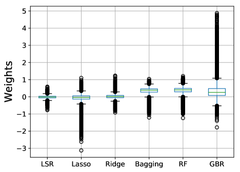
Figure 6: Weight distribution for the GPU kernel performance dataset.

4.2 Music year dataset

Table 3 shows the accuracy metrics results for the music year dataset. In this case, the CNNS gave the best results, both in terms of MSE and MAE. For this dataset, Breiman’s stacking was worse than using gradient boosting, one of the base regressors. The same happens with the usual meta-regression neural network approach. On the other hand, NNS could find a representation that combines the already powerful GBR estimator with less powerful ones in a way that leverages their individual performance.

All base estimators had high prediction error correlations (Table 4). In particular, two of the linear estimators could be removed from the stacking without affecting its performance. However, when removing all three linear estimators the MSE for the best NNS increased to $83.92(\pm 0.57)$ and its MAE increased to $6.44(\pm 0.02)$.

Figure 7 shows that the fitted NNS weights have a large dispersion. This illustrates the flexibility added by our method. Models with very distinctive nature (e.g., ridge regression - which imposes a linear shape on the regression function, and random forests - which is fully non-parametric) can add to each other, getting weights of different magnitudes depending on the region of the feature space that the new instance lies on.

Type Model (Best architecture) MSE MAE Total fit time Stacked estimators UNNS + $\phi_{\mathbf{x}}$ (10 layers) 92.37 ($\pm$ 7.18) 6.53 ($\pm$ 0.02) 9432 CNNS + $\phi_{\mathbf{x}}$ (3 layers) 83.05 ($\pm$ 0.57) 6.38 ($\pm$ 0.02) 8851 UNNS (10 layers) 95.35 ($\pm$ 1.81) 7.45 ($\pm$ 0.02) 12087 CNNS (3 layers) 82.99 ($\pm$ 0.57) 6.38 ($\pm$ 0.02) 11466 Breiman’s stacking 87.66 ($\pm$ 0.57) 6.61 ($\pm$ 0.02) 3090 Meta-regression neural net (1 layer) 87.64 ($\pm$ 0.59) 6.61 ($\pm$ 0.02) 571 Direct estimator Direct neural net (1 layer) 1596.2 ($\pm$ 10.88) 29.83 ($\pm$ 0.07) 2341 Base estimators Least squares 92.03 ($\pm$ 0.62) 6.82 ($\pm$ 0.02) - Lasso 92.61 ($\pm$ 0.62) 6.87 ($\pm$ 0.02) - Ridge 92.03 ($\pm$ 0.62) 6.82 ($\pm$ 0.02) - Bagging 92.83 ($\pm$ 0.59) 6.84 ($\pm$ 0.02) - Random forest 92.6 ($\pm$ 0.59) 6.83 ($\pm$ 0.02) - Gradient boosting 87.49 ($\pm$ 0.6) 6.58 ($\pm$ 0.02) -

Table 3: Evaluation of the model accuracy metrics for the music year dataset.

Models Least squares Lasso Ridge Bagging Random forest Gradient boosting Least squares 1.00 1.00 1.00 0.87 0.87 0.95 Lasso 1.00 1.00 1.00 0.88 0.88 0.96 Ridge 1.00 1.00 1.00 0.87 0.87 0.95 Bagging 0.87 0.88 0.87 1.00 0.89 0.91 Random forest 0.87 0.88 0.87 0.89 1.00 0.91 Gradient boosting 0.95 0.96 0.95 0.91 0.91 1.00

Table 4: Pearson correlation between base estimators prediction errors for the music year dataset.

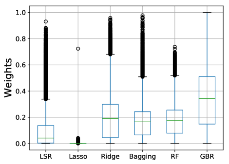
Figure 7: Weight distribution for the music year dataset.

4.3 Blog feedback dataset

Table 5 shows the results for the blog feedback dataset. All stacked estimators had similar performance in terms of MSE. However, UNNS had slightly worse performance with respect to MAE. This may happen because the NNS is designed to minimize the MSE and not the MAE. Overall, for this small dataset, the NNS shows no improvement over Breiman’s stacking or the usual meta-regression neural network.

GBR had the lowest MSE for the base estimators, while bagging and random forests had the lowest MAE. This explains why these models have larger fitted weights (Figure 8). Moreover, the linear models prediction errors had an almost perfect error correlation (Table 6). This suggests that removing up to 2 of them from the NNS would not impact its performance. Also, the linear estimators has a poor performance when compared to the other base regressors. We thus refit the best NNS for this data after removing these estimators, and achieve an MSE of 531.88 ($\pm 62.67$) and a MAE of 5.31 ($\pm 0.20$). We conclude that the linear estimators did not damage nor improved the NNS.

Type Model (Best architecture) MSE MAE Total fit time Stacked estimators UNNS + $\phi_{\mathbf{x}}$ (10 layers) 542.02 ($\pm$ 62.65) 5.89 ($\pm$ 0.2) 420 CNNS + $\phi_{\mathbf{x}}$ (1 layer) 548.99 ($\pm$ 63.9) 5.44 ($\pm$ 0.2) 404 UNNS (10 layers) 557.95 ($\pm$ 61.51) 6.38 ($\pm$ 0.2) 447 CNNS (3 layers) 540.68 ($\pm$ 63.87) 5.44 ($\pm$ 0.2) 433 Breiman’s stacking 593.74 ($\pm$ 73.19) 5.41 ($\pm$ 0.21) 202 Meta-regression neural net (3 layers) 537.66 ($\pm$ 63.31) 5.53 ($\pm$ 0.2) 44 Direct estimator Direct neural net (3 layers) 676.79 ($\pm$ 81.0) 7.52 ($\pm$ 0.22) 63 Base estimators Least squares 878.88 ($\pm$ 109.42) 9.56 ($\pm$ 0.25) - Lasso 877.11 ($\pm$ 108.11) 9.04 ($\pm$ 0.25) - Ridge 877.92 ($\pm$ 109.47) 9.53 ($\pm$ 0.25) - Bagging 619.04 ($\pm$ 88.49) 5.27 ($\pm$ 0.21) - Random forest 585.22 ($\pm$ 64.88) 5.37 ($\pm$ 0.21) - Gradient boosting 557.28 ($\pm$ 63.88) 5.75 ($\pm$ 0.2) -

Table 5: Evaluation of model accuracy metrics for the blog feedback dataset.

Models Least squares Lasso Ridge Bagging Random forest Gradient boosting Least squares 1.00 0.99 1.00 0.68 0.70 0.81 Lasso 0.99 1.00 0.99 0.68 0.69 0.81 Ridge 1.00 0.99 1.00 0.68 0.70 0.81 Bagging 0.68 0.68 0.68 1.00 0.92 0.89 Random forest 0.70 0.69 0.70 0.92 1.00 0.90 Gradient boosting 0.81 0.81 0.81 0.89 0.90 1.00

Table 6: Pearson correlation between base estimators prediction errors for the blog feedback dataset.

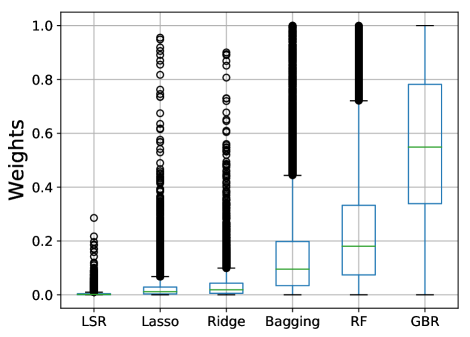
Figure 8: Weight distribution for the blog feedback dataset.

4.4 Superconductivity dataset

The results for the superconductivity dataset (Table 7) were similar to those obtained for the blog feedback data: the NNS methods perform slightly better than Breiman’s in terms of MSE, and worse in terms of MAE. Moreover, both tree-based models had the best MSE among base estimators, competing with the GBR in terms of MAE. Hence, they got larger fitted weights (Figure 9).

Table 8 shows that GBR did not have a high correlation error to the tree-based estimators (0.72 in both cases). This is another reason why although having higher MSE, the GBR has high fitted weight for some instances. One can also note that bagging and random forest had an almost perfect error correlation. This implies that removing one of them would lead to no changes in the NNS. Finally, removing the linear models did not change the MSE and the MAE for the stacking methods.

Type Model (Best architecture) MSE MAE Total fit time Stacked estimators UNNS + $\phi_{\mathbf{x}}$ (10 layers) 98.97 ($\pm$ 4.67) 5.71 ($\pm$ 0.11) 334 CNNS + $\phi_{\mathbf{x}}$ (1 layer) 98.79 ($\pm$ 4.67) 5.65 ($\pm$ 0.11) 325 UNNS (10 layers) 98.62 ($\pm$ 4.77) 5.64 ($\pm$ 0.11) 344 CNNS (3 layers) 98.60 ($\pm$ 4.75) 5.60 ($\pm$ 0.11) 335 Breiman’s stacking 99.79 ($\pm$ 4.95) 5.48 ($\pm$ 0.11) 48 Meta-regression neural net (1 layer) 99.05 ($\pm$ 4.78) 5.60 ($\pm$ 0.11) 24 Direct estimator Direct neural net (3 layers) 274.93 ($\pm$ 7.20) 7.20 ($\pm$ 0.16) 62 Base estimators Least squares 308.65 ($\pm$ 13.41) 7.12 ($\pm$ 0.16) - Lasso 475.6 ($\pm$ 17.08) 9.41 ($\pm$ 0.19) - Ridge 309.17 ($\pm$ 13.42) 7.17 ($\pm$ 0.16) - Bagging 105.14 ($\pm$ 5.68) 5.02 ($\pm$ 0.12) - Random forest 103.02 ($\pm$ 5.59) 5.08 ($\pm$ 0.12) - Gradient boosting 161.48 ($\pm$ 8.74) 5.05 ($\pm$ 0.13) -

Table 7: Evaluation of model accuracy metrics for the superconductivity dataset.

Models Least squares Lasso Ridge Bagging Random forest Gradient boosting Least squares 1.00 0.80 1.00 0.52 0.51 0.78 Lasso 0.80 1.00 0.80 0.45 0.44 0.67 Ridge 1.00 0.80 1.00 0.52 0.51 0.78 Bagging 0.52 0.45 0.52 1.00 0.91 0.72 Random forest 0.51 0.44 0.51 0.91 1.00 0.72 Gradient boosting 0.78 0.67 0.78 0.72 0.72 1.00

Table 8: Pearson correlation between base estimators prediction errors for the superconductivity dataset.

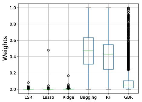
Figure 9: Weight distribution for the superconductivity dataset.

5 Conclusion and future extensions

NN-Stacking is a stacking tool with good predictive power that keeps the simplicity in interpretation of Breiman’s method. The key idea of the method is to take advantage of the fact that distinct base models often perform better at different regions of the feature space, and thus it allows the weight associated to each model to vary with ${\mathbf{x}}$.

Our experiments show that both CNNS and UNNS can be suitable in different settings: in cases where the base estimators do not capture the complexity from the whole data, the freedom adopted by UNNS can lead to a larger improvement in performance. On the other hand, when base estimators already have high performance, UNNS the CNNS have similar predictive power, but the restrictions imposed by CNNS guarantee a more interpretable solution. Both CNNS and UNNS have comparable computational cost.

In our experiments, we observe that NNS improves over standard stacking approaches especially on large datasets. This can be explained by the fact that NNS methods have a higher complexity (i.e., larger number of parameters) than the other approaches. Thus, a larger sample size is needed to satisfactorily estimate them. The experiments also show that including weak regression methods (such as linear methods) might decrease the errors of NNS. In a few cases, however, adding such weak regressors slightly increases the prediction errors of the stacked estimators This suggests that adding a penalization to the loss function that encourages $\theta_{i}$’s to be zero may lead to improved results.

Future work includes extending these ideas to classification problems, as well as developing a leave-one-out version based on super learners [22]. Also, we desire to develop a method of regularization on population moments estimation to avoid over-fitting, as well as to study asymptotic properties for the estimator of $L_{\mathbf{x}}$.

References

Appendix A Proofs

Theorem 3.1. Notice that

$$R(G_{\theta})={\textbf{E}}\left[{\textbf{E}}\left[\left(Y-G_{\theta}({\mathbf{X}})\right)^{2}\right|{\mathbf{X}}]\right].$$

Hence, in order to minimize $R(G_{\theta})$, it suffices to minimize ${\textbf{E}}\left[\left(Y-G_{\theta}({\mathbf{x}})\right)^{2}\right|{\mathbf{X}}={\mathbf{x}}]$ for each ${\mathbf{x}}\in\mathcal{X}$. Now, once $\sum_{i=1}^{k}\theta_{i}(x)=1$, it follows that,

$${\textbf{E}}\left[\left(Y-G_{\theta}({\mathbf{x}})\right)^{2}|{\mathbf{X}}={\mathbf{x}}\right] ={\textbf{E}}\left[\left(\sum_{i=1}^{k}\theta_{i}({\mathbf{x}})(Y-g_{i}({\mathbf{x}}))\right)^{2}|{\mathbf{X}}={\mathbf{x}}\right]$$

$$=\sum_{i,j}\theta_{i}({\mathbf{x}})\theta_{j}({\mathbf{x}}){\textbf{E}}\left[(Y-g_{i}({\mathbf{x}}))(Y-g_{j}({\mathbf{x}}))|{\mathbf{X}}={\mathbf{x}}\right]$$

$$=\theta_{\mathbf{x}}^{t}\mathbb{M}_{\mathbf{x}}\theta_{\mathbf{x}},$$

where $\theta_{\mathbf{x}}=(\theta_{1}({\mathbf{x}}),\ldots,\theta_{k}({\mathbf{x}}))^{\prime}$. Using Lagrange multipliers, the optimal weights can by found by minimizing

$$f(\theta_{\mathbf{x}},\lambda):=\theta_{\mathbf{x}}^{t}\mathbb{M}_{\mathbf{x}}\theta_{\mathbf{x}}-\lambda(\mathbf{e}^{t}\theta_{\mathbf{x}}-1).$$ (A.1)

Now,

$$\frac{\partial f(\theta_{\mathbf{x}},{\mathbf{x}})}{\partial\theta_{\mathbf{x}}}=2\mathbb{M}_{\mathbf{x}}\theta_{\mathbf{x}}-\lambda\mathbf{e},$$

and therefore the optimal solution satisfies $\theta^{*}_{\mathbf{x}}=\frac{\lambda}{2}\mathbb{M}_{\mathbf{x}}^{-1}\mathbf{e}$. Substituting this on Equation A.1 , obtain that

$$f(\theta^{*}_{\mathbf{x}},\lambda)=-\frac{\lambda^{2}}{4}\mathbf{e}^{t}\mathbb{M}_{\mathbf{x}}^{-1}\mathbf{e}+\lambda,$$

and hence

$$\frac{\partial f(\theta^{*}_{\mathbf{x}},\lambda)}{\partial\lambda}=0\iff\lambda=\frac{2}{\mathbf{e}^{t}\mathbb{M}_{\mathbf{x}}^{-1}\mathbf{e}},$$

which yields the optimal solution

$$\theta^{*}_{\mathbf{x}}=\frac{\lambda}{2}\mathbb{M}_{\mathbf{x}}^{-1}\mathbf{e}=\frac{2}{\mathbf{e}^{t}\mathbb{M}_{\mathbf{x}}^{-1}\mathbf{e}}\frac{1}{2}\mathbb{M}_{\mathbf{x}}^{-1}\mathbf{e}=\frac{\mathbb{M}^{-1}_{\mathbf{x}}\mathbf{e}}{\mathbf{e}^{t}\mathbb{M}^{-1}_{\mathbf{x}}\mathbf{e}}.$$

References

- Breiman [1996] Leo Breiman. Stacked regressions. Machine learning, 24(1):49–64, 1996.
- Džeroski and Ženko [2004] Saso Džeroski and Bernard Ženko. Is combining classifiers with stacking better than selecting the best one? Machine learning, 54(3):255–273, 2004.
- Dietterich [2000] Thomas G Dietterich. Ensemble methods in machine learning. In International workshop on multiple classifier systems, pages 1–15. Springer, 2000.
- Sill et al. [2009] Joseph Sill, Gábor Takács, Lester Mackey, and David Lin. Feature-weighted linear stacking. arXiv preprint arXiv:0911.0460, 2009.
- Zhou [2012] Zhi-Hua Zhou. Ensemble methods: foundations and algorithms. CRC press, 2012.
- Fan and Gijbels [1992] Jianqing Fan and Irene Gijbels. Variable bandwidth and local linear regression smoothers. The Annals of Statistics, pages 2008–2036, 1992.
- Breiman [2001] Leo Breiman. Random forests. Machine learning, 45(1):5–32, 2001.
- Csáji [2001] Balázs Csanád Csáji. Approximation with artificial neural networks. Faculty of Sciences, Etvs Lornd University, Hungary, 24:48, 2001.
- Kingma and Ba [2014] Diederik P. Kingma and Jimmy Ba. Adam: A method for stochastic optimization. CoRR, abs/1412.6980, 2014.
- Glorot and Bengio [2010] Xavier Glorot and Yoshua Bengio. Understanding the difficulty of training deep feedforward neural networks. Journal of Machine Learning Research - Proceedings Track, 9:249–256, 01 2010.
- Clevert et al. [2015] Djork-Arné Clevert, Thomas Unterthiner, and Sepp Hochreiter. Fast and accurate deep network learning by exponential linear units (elus), 2015.
- Ioffe and Szegedy [2015] Sergey Ioffe and Christian Szegedy. Batch normalization: Accelerating deep network training by reducing internal covariate shift. In Francis Bach and David Blei, editors, Proceedings of the 32nd International Conference on Machine Learning, volume 37 of Proceedings of Machine Learning Research, pages 448–456, Lille, France, 07 2015. PMLR. URL http://proceedings.mlr.press/v37/ioffe15.html.
- Hinton et al. [2012] Geoffrey E. Hinton, Nitish Srivastava, Alex Krizhevsky, Ilya Sutskever, and Ruslan R. Salakhutdinov. Improving neural networks by preventing co-adaptation of feature detectors. CoRR, 2012.
- Paszke et al. [2017] Adam Paszke, Sam Gross, Soumith Chintala, Gregory Chanan, Edward Yang, Zachary DeVito, Zeming Lin, Alban Desmaison, Luca Antiga, and Adam Lerer. Automatic differentiation in pytorch, 2017.
- Nugteren and Codreanu [2015] Cedric Nugteren and Valeriu Codreanu. Cltune: A generic auto-tuner for opencl kernels. In 2015 IEEE 9th International Symposium on Embedded Multicore/Many-core Systems-on-Chip, pages 195–202. IEEE, 2015.
- Dheeru and Karra Taniskidou [2017] Dua Dheeru and Efi Karra Taniskidou. UCI machine learning repository, 2017. URL http://archive.ics.uci.edu/ml.
- Buza [2014] Krisztian Buza. Feedback prediction for blogs. In Data analysis, machine learning and knowledge discovery, pages 145–152. Springer, 2014.
- Hamidieh [2018] Kam Hamidieh. A data-driven statistical model for predicting the critical temperature of a superconductor. arXiv preprint arXiv:1803.10260, 2018.
- Friedman et al. [2001] Jerome Friedman, Trevor Hastie, and Robert Tibshirani. The elements of statistical learning, volume 1. Springer series in statistics New York, NY, USA:, 2001.
- Meir and Rätsch [2003] Ron Meir and Gunnar Rätsch. An introduction to boosting and leveraging. In Advanced lectures on machine learning, pages 118–183. Springer, 2003.
- Pedregosa et al. [2011] F. Pedregosa, G. Varoquaux, A. Gramfort, V. Michel, B. Thirion, O. Grisel, M. Blondel, P. Prettenhofer, R. Weiss, V. Dubourg, J. Vanderplas, A. Passos, D. Cournapeau, M. Brucher, M. Perrot, and E. Duchesnay. Scikit-learn: Machine learning in Python. Journal of Machine Learning Research, 12:2825–2830, 2011.
- Van der Laan et al. [2007] Mark J Van der Laan, Eric C Polley, and Alan E Hubbard. Super learner. Statistical applications in genetics and molecular biology, 6(1), 2007.