Deep Residual Learning for Image Compression

Abstract

In this paper, we provide a detailed description on our approach designed for CVPR 2019 Workshop and Challenge on Learned Image Compression (CLIC). Our approach mainly consists of two proposals, i.e. deep residual learning for image compression and sub-pixel convolution as up-sampling operations. Experimental results have indicated that our approaches, Kattolab, Kattolabv2 and KattolabSSIM, achieve 0.972 in MS-SSIM at the rate constraint of 0.15bpp with moderate complexity during the validation phase.

1 Introduction

Image compression has been an significant task in the field of signal processing for many decades to achieve efficient transmission and storage. Classical image compression standards, such as JPEG [1], JPEG2000 [2] and HEVC/H.265-intra [3], usually rely on hand-crafted encoder/decoder (codec) block diagrams. Along with the fast development of new image formats and high-resolution mobile devices, existing image compression standards are not expected to be optimal and general compression solutions.

Recently, we have seen a great surge of deep learning based image compression works. Some approaches use generative models to learn the distribution of images using adversarial training [4, 5, 6]. They can achieve better subjective quality at extremely low bit rate. Some works use recurrent neural networks to compress the residual information recursively, such as [7, 8, 9]. These works are progressive coding, which can compress images at different quality levels at once. More approaches on relaxations of quantization and estimations of entropy model have been proposed in [10, 11, 12, 13, 14, 15, 16, 17, 18, 19]. Their ideas include using differentiable quantization approximation, or estimating the distribution for latent codes as entropy models, or de-correlating different channels for latent representation. Promising results have been achieved compared with classical image compression standards.

However, selecting a proper network structure is a daunting task for all types of machine learning tasks, including learned image compression. In this paper, we mainly discuss two issues. The first is about the kernel size. In classical image compression algorithms, filter sizes are quite important. Motivated from this, we conduct some experiments with different filter sizes to find larger kernel size contributes to better coding efficiency. Based on this observation, we propose to utilize deep residual learning to maintain the same receptive field with fewer parameters. This strategy not only reduces the model size, but also improves the performance greatly. On the other hand, the design of up-sampling operations at the decoder side is also significant to determine the reconstructed image quality and the type of artifacts. This issue has been widely discussed in super resolution tasks, and up-sampling layers can be implemented in various ways, such as interpolation, transposed convolution, sub-pixel convolution. We compare two popular up-sampling operations, i.e. transposed convolution and sub-pixel convolution to illustrate their performance.

In CLIC 2019, we submitted three entries including Kattolab, Kattolabv2, and KattolabSSIM in the low rate track, to achieve 0.972 MS-SSIM with moderate complexity.

2 Deep Residual Learning for Image Compression with Sub-Pixel Convolution

The network architectures that we used as anchors are illustrated in Fig. 1. This architecture is referred from the work [12] and the work [14], which has achieved the state-of-the-art compression efficiency. The network consists of two autoencoders. The main autoencoder controls the rate-distortion optimization for image compression, and the loss function is formulated as

$$J=\lambda d(\boldsymbol{x},\hat{\boldsymbol{x}})+R(\hat{\boldsymbol{y}})$$ (1)

where $\lambda$ controls the tradeoff between the rate and distortion. The auxiliary autoencoder is used to encode the side information to model the distribution of compressed information. Gaussian scale mixture is used to estimate an image-dependent and adaptive entropy model, where scale parameters are conditioned on a hyperprior. Moreover, [14] proposed a joint autoregressive and hyperprior approach, denoted as Joint. The only difference is to append a masked $5\times 5$ convolution after quantization and to concatenate the output of auxiliary autoencoder and masked convolution together to learn the entropy model.

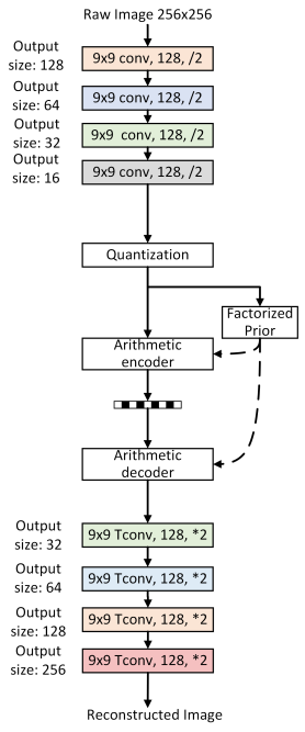
(a) Baseline-9

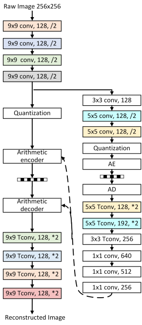
(b) HyperPrior-9

Figure 1: The network structure of anchors we used.

2.1 From Small Kernel Size to Large Kernel Size

In classical image compression algorithms, transform filter sizes are quite important to improve the coding efficiency, especially for UHD videos. From the smallest transform size $4\times 4$, larger and larger transform size is gradually used into video coding algorithms. Specifically, up to $32\times 32$ DCT coefficients have been incorporated into HEVC [3]. Large kernel size brings benefits on capturing the spatial correlation and semantic information. Motivated from this, we conduct some experiments using Kodak dataset [26] with different filter sizes in the main and auxiliary autoencoders respectively to explore the effect of larger kernel size on coding efficiency. Table 1 shows for the Baseline architecture, along with the increasing of kernel sizes, the rate-distortion performance are becoming better. Table 2 demonstrate similar results for HyperPrior architectures. Table 3 shows large kernel in the auxiliary autoencoder cannot bring any benefits on RD performance and even gets worse, because the compressed codes $y$ has small size, so $5\times 5$ are large enough. Too many learnable parameters instead increase the difficulty to learn. It is worth noting for Joint architecture [14], a sequential decoding is inevitable, which is extremely time-consuming when the test image becomes larger. Therefore, we exclude the masked convolution in this challenge, but keep the $1\times 1$ conv as they are, for HyperPrior architecture. An ablation on the effect of $1\times 1$ conv will be conducted in the future.

Table 1: The effect of kernel size on Baseline on Kodak, optimized by MSE with $\lambda=0.015$.

Method	PSNR	MS-SSIM	Rate
Baseline-3	32.160	0.9742	0.671
Baseline-5	32.859	0.9766	0.641
Baseline-9	32.911	0.9776	0.633

Table 2: The effect of kernel size on HyperPrior on Kodak, optimized by MSE with $\lambda=0.015$.

Method	PSNR	MS-SSIM	Rate
HyperPrior-3	32.488	0.9742	0.543
HyperPrior-5	32.976	0.9757	0.518
HyperPrior-9	33.005	0.9765	0.512

Table 3: The effect of kernel size in the auxiliary autoencoder on Kodak, optimized by MS-SSIM with $\lambda=5$.

Method	PSNR	MS-SSIM	Rate
HyperPrior-9-Aux-5	26.266	0.9591	0.169
HyperPrior-9-Aux-9	26.236	0.9590	0.171

2.2 From Shallow Network to Deep Residual Network

With respect to the receptive field, the stack of four $3\times 3$ kernels capture the same receptive field as one $9\times 9$ kernel with fewer parameters. We have tried to replace one large kernel with several $3\times 3$ filters, however, experiment shows the stack of $3\times 3$ kernels cannot converge. Motivated from [20], we add the shortcut connection for neighboring $3\times 3$ kernels. Our proposed deep residual network for image compression is shown in Fig. 2. Fig. 2(a) is denoted as 3$\times$3(3), where the stack of three $3\times 3$ kernels reaches the same receptive field as 7$\times$7. The architecture of Fig. 2(b) is ResNet-3$\times$3(4), where the stack of four $3\times 3$ kernels reaches the same receptive field as 9$\times$9. As for the activation functions, to prevent more parameters overhead, we only use GDN/IGDN [11] for one time in each residual unit when the output size changes. For other convolutional layers, we use parameter-free Leaky ReLU as activation function to add the non-linearity in the networks. The shortcut projection is shown in Fig. 3. As shown in Table 4, ResNet-3$\times$3(4) is better than ResNet-3$\times$3(3) and Hyperprior-9.

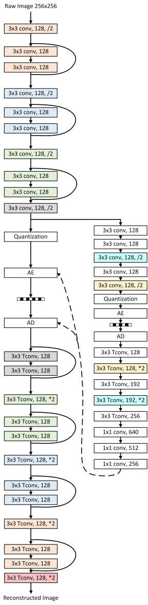
(a) ResNet-3$\times$3(3)

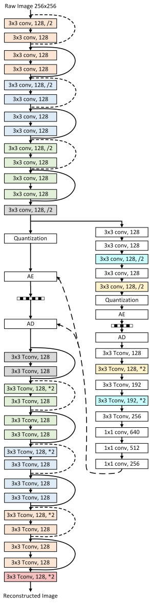
(b) ResNet-3$\times$3(4)

Figure 2: Network structure of proposed deep residual learning, where the solid and dotted lines denote the shortcut connection without and with size change, respectively.

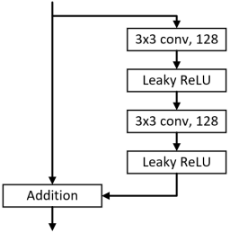
(a) Without size change

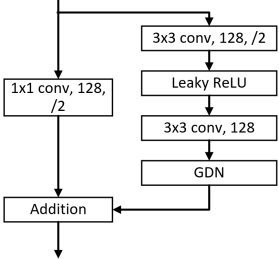
(b) With size change

Figure 3: The network structure of one residual unit.

2.3 Upsampling Operations at Decoder Side

The encoder-decoder pipeline is a symmetric architecture. The down-sampling operations at the encoder side are intuitively implemented using convolution filters with stride, however, up-sampling operations at the decoder side have various ways, including bicubic interpolation [21], transposed convolution [22], sub-pixel convolution[23]. Typically, almost all the previous works use the transposed convolution (TConv), except for the work [10] use sub-pixel convolution at the decoder side. Considering for fast end-to-end learning, we exclude bicubic interpolation and compare two popular up-sampling operations, i.e. TConv and Sub-pixel Conv. For sub-pixel conv, we increase the number of channels by 4 times and then use tf.depth_to_space function in Tensorflow. Results in Table. 4 show sub-pixel convolution filters bring some improvement on PSNR and MS-SSIM than transposed convolution filters.

Table 4: Comparison of residual networks and upsampling operations on Kodak, optimized by MS-SSIM with $\lambda=5$.

Method	PSNR	MS-SSIM	Rate
Hyperprior-9	26.266	0.9591	0.1690
ResNet-3$\times$3(3)	26.378	0.9605	0.1704
ResNet-3$\times$3(4)-TConv	26.457	0.9611	0.1693
ResNet-3$\times$3(4)-SubPixel	26.498	0.9622	0.1700

Table 5: The effect of wide bottleneck on Kodak dataset.

Method	PSNR	MS-SSIM	Rate
ResNet-3x3(4)-Bottleneck128	26.498	0.9622	0.1700
ResNet-3x3(4)-Bottleneck192	26.317	0.9619	0.1667

Table 6: Rate control on CLIC validation dataset [27].

Method	$\boldsymbol{\lambda}$	PSNR	MS-SSIM	Rate
ResNet-3x3(4)-Bottleneck192	5	29.708	0.9697	0.1369
ResNet-3x3(4)-Bottleneck192	10	30.710	0.9765	0.1816

Table 7: Results on CLIC validation dataset [27].

Entry	Description	PSNR	MS-SSIM	Rate
Kattolab	HyperPrior-9	28.902	0.9674	0.134
Kattolab	HyperPrior-9 + Rate Control	29.102	0.9701	0.150
Kattolab	ResNet-3$\times$3(4)-TConv + Rate Control	29.315	0.9716	0.150
Kattolabv2	ResNet-3$\times$3(4)-SubPixel+ Rate Control	29.300	0.9720	0.150
KattolabSSIM	ResNet-3$\times$3(4)-SubPixel + Wide Bottleneck + Rate Control	29.211	0.9724	0.150

3 Implementation Details

For training, we use $256\times 256$ patches cropped from ILSVRC validation dataset (ImageNet [24]). Batch size is 8, and up to 2M iterations are conducted to reach stable results. The model was optimized using Adam [25], and the learning rate was maintained at a fixed value of $1\times 10^{-4}$ and was reduced to $1\times 10^{-5}$ for the last 80K iterations.

We also use two strategies for CLIC2019. One is Wide Bottleneck. More filters can increase the model capacity. Regarding that increasing the number of filters for large feature maps will significantly increase FLOPs, we only increase the number of filters in the last layer of encoder from 128 to 192, so that FLOPs are only increased a little, from $2.50\times 10^{10}$ to $2.56\times 10^{10}$. Results are compared in Table. 5. Bottleneck192 reduces the bitrate a lot, but also degrades quality compared to Bottleneck128.

The other is Rate Control. For the low-rate track, 0.15bpp is the hard threshold. We train two models at different bit rates by adjusting $\lambda$, where the averaged rate with $\lambda=5$ is less than 0.15bpp for the validation dataset, and the averaged rate with $\lambda=8$ is larger than 0.15bpp. Results are shown in Table. 6. Then we can encode all the test images twice and select adaptive to push the rate to 0.15bpp with the maximized MS-SSIM. One bit should be added into the bitstream to specify which model is used for decoding, which will not increase the complexity of the decoder.

4 Result Analysis

The compression results of our approaches on CLIC validation dataset are summarized in Table 7.

Although deep residual network brings the coding gain, the model size grows significantly. In this section, we will analyze the number of parameters and the model complexity with respect to floating point operations per second (FLOPs) for all kinds of architectures. Specifically, take the architecture HyperPrior-9 as an example, the layer-wise model size analysis is illustrated in Table 8. The number of parameters and FLOPs are calculated by

$$\text{Para}=(h\times w\times C_{in}+1)\times C_{out}$$ (2)

$$\text{FLOPs}=\text{Para}\times H^{\prime}\times W^{\prime}$$

where $h\times w$ is the kernel size, $H^{\prime}\times W^{\prime}$ is the output size. $C_{in}$ and $C_{out}$ are the number of channels before or after one operation. If no bias is applied, the $+1$ are removed, such as conv4. Quantization and leaky-ReLU are parameter-free. GDN [13] only run across different channels, but not across different spatial positions, the number of parameters of GDN is only $(C_{in}+1)\times C_{out}$. FLOPs of the total GDN and inverse GDN calculation is only 7.10$\times 10^{8}$. This paper mainly focus on the backbone of convolutional layers, so we omit the FLOPs of GDN, inverse GDN and factorized prior. The comparison is listed in Table 9, where the last column is relative value of FLOPs using Baseline-5 [11] as a baseline model. ResNet-3$\times$3(4) also denotes ResNet-3$\times$3(4)-TConv. Our models achieve better coding performance with low complexity.

Table 8: The model size analysis of HyperPrior-9.

Layer	Kernel		Channel		Output		Para	FLOPs
	h	w	$C_{in}$	$C_{out}$	$H^{\prime}$	$W^{\prime}$
conv1	9	9	3	128	128	128	31232	5.12$\times 10^{8}$
conv2	9	9	128	128	64	64	1327232	5.44$\times 10^{9}$
conv3	9	9	128	128	32	32	1327232	1.36$\times 10^{9}$
conv4	9	9	128	128	16	16	1327104	3.40$\times 10^{8}$
GDN/IGDN							99072	-
Hconv1	3	3	128	128	16	16	147584	3.78$\times 10^{7}$
Hconv2	5	5	128	128	8	8	409728	2.62$\times 10^{7}$
Hconv3	5	5	128	128	4	4	409728	6.56$\times 10^{6}$
FactorizedPrior							5888	-
HTconv1	5	5	128	128	8	8	409728	2.62$\times 10^{7}$
HTconv2	5	5	128	192	16	16	614592	1.57$\times 10^{8}$
HTconv3	3	3	192	256	16	16	442624	1.13$\times 10^{8}$
layer1	1	1	256	640	16	16	164480	4.21$\times 10^{7}$
layer2	1	1	640	512	16	16	328192	8.40$\times 10^{7}$
layer3	1	1	512	256	16	16	131072	3.36$\times 10^{7}$
Tconv1	9	9	128	128	32	32	1327232	1.36$\times 10^{9}$
Tconv2	9	9	128	128	64	64	1327232	5.44$\times 10^{9}$
Tconv3	9	9	128	128	128	128	1327232	2.17$\times 10^{10}$
Tconv4	9	9	128	128	256	256	31107	2.04$\times 10^{9}$
Total							11188291	3.88$\boldsymbol{\times 10^{10}}$

Table 9: The model complexity of different architectures.

Method	Para	FLOPs	Relative
Baseline-3	997379	4.25$\times 10^{9}$	0.36
Baseline-5	2582531	1.18$\times 10^{10}$	1.00
Baseline-9	8130563	3.82$\times 10^{10}$	3.24
HyperPrior-3	4055107	4.78$\times 10^{9}$	0.40
HyperPrior-5	5640259	1.23$\times 10^{10}$	1.04
HyperPrior-9	11188291	3.88$\times 10^{10}$	3.28
ResNet-3$\times$3(3)	5716355	1.75$\times 10^{10}$	1.48
ResNet-3$\times$3(4)	6684931	2.43$\times 10^{10}$	2.06
ResNet-3$\times$3(4)-SubPixel	8172172	2.50$\times 10^{10}$	2.12
ResNet-3$\times$3(4)-SubPixel-Bottleneck192	11627916	2.56$\times 10^{10}$	2.17

5 Conclusion

In this paper, we have described the proposed deep residual learning and sub-pixel convolution for image compression. This is the basis of our submitted entries Kattolab, Kattolabv2 and KattolabSSIM. Results have shown our approaches achieve 0.972 in MS-SSIM at the rate of 0.15bpp with moderate complexity during the validation phase.

References

- [1] G. K Wallace, “The JPEG still picture compression standard”, IEEE Trans. on Consumer Electronics, vol. 38, no. 1, pp. 43-59, Feb. 1991.
- [2] Majid Rabbani, Rajan Joshi, “An overview of the JPEG2000 still image compression standard”, ELSEVIER Signal Processing: Image Communication, vol. 17, no, 1, pp. 3-48, Jan. 2002.
- [3] G. J. Sullivan, J. Ohm, W. Han and T. Wiegand, “Overview of the High Efficiency Video Coding (HEVC) Standard”, IEEE Transactions on Circuits and Systems for Video Technology, vol. 22, no. 12, pp. 1649-1668, Dec. 2012.
- [4] Ripple Oren, L. Bourdev, “Real Time Adaptive Image Compression”, Proc. of Machine Learning Research, Vol. 70, pp. 2922-2930, 2017.
- [5] S. Santurkar, D. Budden, N. Shavit, “Generative Compression”, Picture Coding Symposium, June 24-27, 2018.
- [6] E. Agustsson, M. Tschannen, F. Mentzer, R. Timofte, and L. V. Gool, “Generative Adversarial Networks for Extreme Learned Image Compression”, arXiv:1804.02958.
- [7] G. Toderici, S. M.O’Malley, S. J. Hwang, et al., “Variable rate image compression with recurrent neural networks”, arXiv: 1511.06085, 2015.
- [8] G, Toderici, D. Vincent, N. Johnson, et al., “Full Resolution Image Compression with Recurrent Neural Networks”, IEEE Conf. on Computer Vision and Pattern Recognition (CVPR), pp. 1-9, July 21-26, 2017.
- [9] Nick Johnson, Damien Vincent, David Minnen, et al., “Improved Lossy Image Compression with Priming and Spatially Adaptive Bit Rates for Recurrent Networks”, arXiv:1703.10114, pp. 1-9, March 2017.
- [10] Lucas Theis, Wenzhe Shi, Andrew Cunninghan and Ferenc Huszar, “Lossy Image Compression with Compressive Autoencoders”, Intl. Conf. on Learning Representations (ICLR), pp. 1-19, April 24-26, 2017.
- [11] J. Balle, Valero Laparra, Eero P. Simoncelli, “End-to-End Optimized Image Compression”, Intl. Conf. on Learning Representations (ICLR), pp. 1-27, April 24-26, 2017.
- [12] J. Balle, D. Minnen, S. Singh, S. J. Hwang, N. Johnston, “Variational Image Compression with a Hyperprior”, Intl. Conf. on Learning Representations (ICLR), pp. 1-23, 2018.
- [13] J. Balle, “Efficient Nonlinear Transforms for Lossy Image Compression”, Picture Coding Symposium, 2018.
- [14] D. Minnen, J. Balle, G. Toderici, “Joint Autoregressive and Hierarchical Priors for Learned Image Compression”, arXiv.1809.02736.
- [15] E. Agustsson, F. Mentzer, M. Tschannen, L. Cavigelli, R. Timofte, L. Benini, L. V. Gool, “Soft-to-Hard Vector Quantization for End-to-End Learning Compressible Representations”, Neural Information Processing Systems (NIPS) 2017, arXiv:1704.00648v2.
- [16] F. Mentzer, E. Agustsson, M. Tschannen, R. Timofte, L. V. Gool, “Conditional Probability Models for Deep Image Compression”, IEEE Conf. on Computer Vision and Pattern Recognition (CVPR), June 17-22, 2018.
- [17] Z. Cheng, H. Sun, M. Takeuchi, J. Katto, “Deep Convolutional AutoEncoder-based Lossy Image Compression”, Picture Coding Symposium, pp. 1-5, June 24-27, 2018.
- [18] Z. Cheng, H. Sun, M. Takeuchi, J. Katto, “Performance Comparison of Convolutional AutoEncoders, Generative Adversarial Networks and Super-Resolution for Image Compression”, CVPR Workshop and Challenge on Learned Image Compression (CLIC), pp. 1-4, June 17-22, 2018.
- [19] M. Li, W. Zuo, S. Gu, D. Zhao, D. Zhang, “Learning Convolutional Networks for Content-weighted Image Compression”, IEEE Conf. on Computer Vision and Pattern Recognition (CVPR), June 17-22, 2018.
- [20] K. He, X. Zhang, S. Ren and J. Sun, “Deep Residual Learning for Image Recognition”, arXiv.1512.03385, 2015.
- [21] C. Dong, C. C. Loy, K. He, X. tang, “Image Super-resolution using Deep Convolutional Networks”, arXiv.1501.00092.
- [22] C. Dong, C. C. Loy, X. tang, “Accelerating the Super-Resolution Convolutional Neural Network”. arXiv.1608.00367.
- [23] W. Shi, J. Caballero, F. Huszar, et al. “Real-time single image and video super-resolution using an efficient sub-pixel convolutional neural network”, Intl. IEEE Conf. on Computer Vision and Pattern Recognition, June 26-July 1, 2016.
- [24] J. Deng, W. Dong, R. Socher, L. Li, K. Li and L. Fei-Fei, “ImageNet: A Large-Scale Hierarchical Image Database”, IEEE Conf. on Computer Vision and Pattern Recognition, pp. 1-8, June 20-25, 2009.
- [25] D. P. Kingma and J. Ba, “Adam: A method for stochastic optimization”, arXiv:1412.6980, pp.1-15, Dec. 2014.
- [26] Kodak Lossless True Color Image Suite, Download from http://r0k.us/graphics/kodak/
- [27] Workshop and Challenge on Learned Image Compression, CVPR2019, http://www.compression.cc/