BFKL equation in the next-to-leading order: solution at large impact parameters.

Abstract

In this paper, we show (i) that the NLO corrections do not change the power-like decrease of the scattering amplitude at large impact parameter ($b^{2}\,>\,r^{2}\exp\left(2\bar{\alpha}_{S}\eta(1+4\bar{\alpha}_{S})\right)$, where $r$ denotes the size of scattering dipole and $\eta\,=\,\ln\left(1/x_{Bj}\right)$ for DIS), and, therefore, they do not resolve the inconsistency with unitarity; and (ii) they lead to an oscillating behaviour of the scattering amplitude at large $b$, in direct contradiction with the unitarity constraints.

However, from the more practical point of view, the NLO estimates give a faster decrease of the scattering amplitude as a function of $b$, and could be very useful for description of the experimental data. It turns out, that in a limited range of $b$, the NLO corrections generates the fast decrease of the scattering amplitude with $b$, which can be parameterized as $N\,\propto\,\exp\left(-\,\mu\,b\right)$ with $\mu\,\propto\,1/r$ in accord with the numerical estimates in Ref.CCM .

I Introduction

This paper is motivated and triggered by the result of the numerical solutionCCM of the Balitsky-Kovchegov(BK) equation in the next-to-leading order (NLO), in which at large impact parameter, the solution shows an exponential decrease ($\propto\exp\left(-\mu\,b\right)$). Since the amplitude decreases at large $b$, the non-linear term in the BK equation is small and can be neglected, reducing the problem of large $b$ behaviour, to the solution of the BFKL equation. The large impact parameter behaviour of the scattering amplitude remains the most fundamental problem, which is still unsolvedKW1 ; KW2 ; KW3 in the frame of the CGC/saturation approach (see Ref.KOLEB for a review). Indeed, in the CGC/saturation approach, the scattering amplitude decreases as a power of $b$ KW1 ; KW2 ; KW3 contradicting the Froissart theoremFROI . The intensive attempts to solve this problem and introduce the non-perturbative corrections, which bring the dimensional scale into the problemLERYSL ; GBS1 ; GKLMN ; BEST1 ; BEST2 ; BEST0 ; LETA ; LLS ; LESL , results in the widely held opinion, that we need to introduce a new non-perturbative dimensional scale in the kernel of the BFKL equation. With this in mind, the result of Ref.CCM looks strange, since the NLO kernel, that has been used in the paper, has conformal symmetry, and no dimensional scale has been introduced.

The goal of this paper is to show, that in NLO we still have power-like behaviour at large values of $b$, as the result of the conformal symmetry of the BFKL kernel. However, we find that there is a kinematic region where the solution has a fast decrease with $b$ ($\propto\,e^{-\mu b}$) and this falloff can be parameterized as an exponential with $\mu\,\propto\,1/r$, where $r$ denotes the size of the scattering dipole.

The paper is organized as follows. In the next section we discuss general features of the BFKL Pomeron at large values of the impact parameter. In Section 3, we discuss the impact parameter dependence in double log approximation (DLA) of the leading order of the BFKL evolution equation, and show that the scattering amplitude decreases as a power of $b$. Section 4 is the main part of the paper and it deals with the DLA for the next-to-leading (NLA) BFKL evolution equation. We show that the solution for $b^{2}\,>\,r^{2}\exp\left(\frac{1}{2}\eta\right)$, where $\eta=\ln\left(1/x_{Bj}\right)$ in DIS, not only has power-like decrease as function of $b$, but leads to an oscillating function, which contradicts unitarity constraints. In section 5 we argue that the main features of the DLA will be preserved in a more general approach. In the conclusion we discuss our findings, and emphasize that we need to introduce the new dimensional scale into the BFKL kernel , which is related to the non-perturbative corrections, that resolve the difficulties at large $b$ in the framework of the CGC approach. On the other hand, we note that the NLO corrections suppress the scattering amplitude, and could possibly be useful for the description of the experimental data (see Ref.CCM ).

II BFKL Pomeron

The BFKL evolution equation for the dipole-target scattering amplitude $N\left(\boldsymbol{x}_{10},\boldsymbol{b},Y\right)$ has the general formKOLEB ; BFKL ; LIP :

$$\frac{\partial}{\partial Y}N\left(\boldsymbol{x}_{10},\boldsymbol{b},Y\right)=$$ (1)

$$\bar{\alpha}_{S}\!\!\int\frac{d^{2}\boldsymbol{x}_{2}}{2\,\pi}\,K\left(\boldsymbol{x}_{02},\boldsymbol{x}_{12};\boldsymbol{x}_{10}\right)\left(N\left(\boldsymbol{x}_{12},\boldsymbol{b}-\frac{1}{2}\boldsymbol{x}_{20},Y\right)+N\left(\boldsymbol{x}_{20},\boldsymbol{b}-\frac{1}{2}\boldsymbol{x}_{12},\eta\right)-N\left(\boldsymbol{x}_{10},\boldsymbol{b},Y\right)\right)$$

where $\boldsymbol{x}_{ik}\,\,=\,\,\boldsymbol{x}_{i}\,-\,\boldsymbol{x}_{k}$ and $\boldsymbol{x}_{10}\equiv\,\boldsymbol{r}$, $\boldsymbol{x}_{20}\,\equiv\,\boldsymbol{r}^{\prime}$ and $\boldsymbol{x}_{12}\,\equiv\,\boldsymbol{r}\,-\,\boldsymbol{r}^{\prime}$. $Y$ is the rapidity of the scattering dipole and $\boldsymbol{b}$ is the impact factor. $K\left(\boldsymbol{x}_{02},\boldsymbol{x}_{12};\boldsymbol{x}_{10}\right)$ is the kernel of the BFKL equation which in leading order has the following form:

$$K_{\rm LO}\left(\boldsymbol{x}_{02},\boldsymbol{x}_{12};\boldsymbol{x}_{10}\right)\,\,=\,\,\frac{x^{2}_{10}}{x^{2}_{02}\,x^{2}_{12}}$$ (2)

In Ref.LIP it has been proved that the eigenfunction of the BFKL equation has the following form

$$\phi_{\gamma}\left(\boldsymbol{r},\boldsymbol{R},\boldsymbol{b}\right)\,\,\,=\,\,\,\left(\frac{r^{2}\,R^{2}}{\left(\boldsymbol{b}+\frac{1}{2}(\boldsymbol{r}-\boldsymbol{R})\right)^{2}\,\left(\boldsymbol{b}-\frac{1}{2}(\boldsymbol{r}-\boldsymbol{R})\right)^{2}}\right)^{\gamma}\,\,\xrightarrow{b\,\gg\,r,R}\,\,\left(\frac{r^{2}\,R^{2}}{b^{4}}\right)^{\gamma}\,\,\equiv\,\,e^{\gamma\,\xi}~{}~{}\mbox{with}~{}~{}\xi\,=\,\ln\left(\frac{r^{2}\,R^{2}}{b^{4}}\right)$$ (3)

for any kernel, which satisfies the conformal symmetry. In Eq. (3) $r$ denotes the size of the scattering dipole, while $R$ is the size of the target. For the kernel of the LO BFKL equation (see Eq. (2)) the eigenvalues take the form:

$$\omega_{\rm LO}\left(\bar{\alpha}_{S},\gamma\right)\,\,=\,\,\bar{\alpha}_{S}\,\chi^{LO}\left(\gamma\right)\,\,\,=\,\,\,\bar{\alpha}_{S}\left(2\psi\left(1\right)\,-\,\psi\left(\gamma\right)\,-\,\psi\left(1-\gamma\right)\right)$$ (4)

$\psi(z)$ denotes the Euler psi-function $\psi\left(z\right)=d\ln\Gamma(z)/dz$.

In the next-to-leading order the kernel is derived in Refs.BFKLNLO ; BFKLNLO1 and has the following form:

$$\omega_{\rm NLO}\left(\bar{\alpha}_{S},\gamma\right)\,\,=\,\,\bar{\alpha}_{S}\,\chi^{LO}\left(\gamma\right)\,\,+\,\,\bar{\alpha}_{S}^{2}\,\chi^{NLO}\left(\gamma\right)$$ (5)

The explicit form of $\chi^{NLO}\left(\gamma\right)$ is given in Ref.BFKLNLO . However, $\chi^{NLO}\left(\gamma\right)$ turns out to be singular at $\gamma\to 1$, $\chi^{NLO}\left(\gamma\right)\,\propto\,1/(1-\gamma)^{3}$. Such singularities indicate, that to obtain a reliable result, it is necessary to calculate higher order corrections . The procedure to re-sum high order corrections is suggested in Ref. SALAM ; SALAM1 ; SALAM2 ; KMRS . The resulting spectrum of the BFKL equation in the NLO, can be found from the solution of the following equation SALAM ; SALAM1 ; SALAM2

$$\omega_{\rm NLO}\left(\bar{\alpha}_{S},\gamma\right)\,=\,\bar{\alpha}_{S}\left(\chi_{0}\left(\omega_{\rm NLO},\gamma\right)\,+\,\omega_{\rm NLO}\,\frac{\chi_{1}\left(\omega_{\rm NLO},\gamma\right)}{\chi_{0}\left(\omega_{\rm NLO},\gamma\right)}\right)$$ (6)

where

$$\chi_{0}\left(\omega,\gamma\right)\,\,=\,\,\chi^{LO}\left(\gamma\right)\,-\,\frac{1}{1\,-\,\gamma}\,+\,\frac{1}{1\,-\,\gamma\,+\,\omega}$$ (7)

and

$$\chi_{1}\left(\omega,\gamma\right)\,\,=$$ (8)

$$\,\,\chi^{NLO}\left(\gamma\right)\,+\,F\left(\frac{1}{1-\gamma}\,-\,\frac{1}{1\,-\,\gamma\,+\,\omega}\right)\,+\,\frac{A_{T}\left(\omega\right)\,-\,A_{T}\left(0\right)}{\gamma^{2}}\,+\,\frac{A_{T}\left(\omega\right)-b}{\left(1\,-\,\gamma\,+\,\omega\right)^{2}}\,-\,\frac{A_{T}\left(0\right)-b}{\left(1\,-\,\gamma\right)^{2}}$$

Functions $\chi^{NLO}\left(\gamma\right)$ and $A_{T}\left(\omega\right)$ as well as the constants ($F$ and $b$) are given in Refs.SALAM ; SALAM1 ; SALAM2 .

In Ref. KMRS a simpler form of $\chi_{1}\left(\omega,\gamma\right)$ was suggested, which coincides with Eq. (8) to within $7\%$, and, therefore, gives reasonable estimates of all constants and functions in Eq. (8). The equation for $\omega$ takes the form

$$\omega\,=\,\bar{\alpha}_{S}\left(1-\omega\right)\left(\frac{1}{\gamma}+\frac{1}{1-\gamma+\omega}\,+\,\underbrace{\left(2\psi(1)-\psi\left(2-\gamma\right)-\psi\left(1+\gamma\right)\right)}_{\mbox{ high twist contributions}}\right)$$ (9)

One can see that $\gamma(\omega)\to 0$ when $\omega\to 1$, as follows from energy conservation.

The general solution to Eq. (1) takes the form:

$$N\left(\xi,Y\right)\,\,\,=\,\,\,\int^{\epsilon+i\infty}_{\epsilon-i\infty}\frac{d\gamma}{2\,\pi\,i}e^{\omega\left(\bar{\alpha}_{S},\gamma\right)\,Y\,\,+\,\,\gamma\,\xi}\,\phi_{\rm in}\left(\gamma\right)$$ (10)

where $\gamma_{\rm in}$ can be found from the initial condition at $\eta=0$. We suggest to take the initial condition in the form:

$$N\left(\xi,Y=0\right)\,=\,\exp\left(-Be^{-\,\frac{1}{2}\xi}\right)\,\,=\,\,\exp\left(-B\frac{b^{2}}{r\,R}\right)$$ (11)

Taking the inverse Mellin transform, we obtain $\phi_{in}$ is equal to

$$\phi_{in}\left(\gamma\right)\,\,=\,\,2\,B^{\,-\,2\,\gamma}\Gamma\left(\,2\,\gamma\right)$$ (12)

One can see that $\phi_{in}$ has a pole at $\gamma=0$. To avoid this pole, which occurs due to our simplifying the estimates, we modify the initial conditions:

$$\phi_{in}\left(\gamma\right)\,\,=2\,\,\left(B_{1}^{-2\,\gamma}\,-\,B_{2}^{-2\,\gamma}\right)\,\Gamma\left(2\,\gamma\right)$$ (13)

Eq. (13) has no singularities at $\gamma=0$, at any value of $B_{1}$ and $B_{2}$.

For large $Y$ and $\xi$ we can use the method of stepest descent in calculating the integral of Eq. (10). The equation for the saddle point ($\gamma=\gamma_{\rm SP}$) is

$$\frac{d\omega\left(\bar{\alpha}_{S},\gamma\right)}{d\gamma}\Big{|}_{\gamma\,=\,\gamma_{\rm SP}}\,\,=\,\,-\,\frac{\xi}{Y}$$ (14)

For large $|\xi|$ ($|\xi|/Y\,\gg\,1)$ at $\gamma=\gamma_{\rm SP}$ $\frac{d\omega\left(\bar{\alpha}_{S},\gamma\right)}{d\gamma}$ should be large. All kernels, that we have discussed in Eq. (4) - Eq. (9) are large at $\gamma\,\to\,1$ and, actually, accounting for this singularity, corresponds to the double log approximation(DLA) of perturbative QCD.

III DLA for LO BFKL equation

For the case of the leading order BFKL equation at $\gamma\,\,\to\,\,1$, $\omega_{\rm LO}\,=\,\frac{\bar{\alpha}_{S}}{1-\gamma}$ and Eq. (14) takes the form

$$\frac{\bar{\alpha}_{S}}{\left(1-\gamma_{\rm SP}\right)^{2}}\,Y\,\,=\,\,-\,\xi$$ (15)

leading to $\bar{\gamma}_{\rm SP}\,\,\equiv\,\,1\,-\,\gamma_{\rm SP}\,=\,\,\sqrt{\frac{\bar{\alpha}_{S}\,Y}{|\xi|}}$. Plugging this solution into Eq. (10) we obtain that

$$N\left(Y,\xi\right)\,\,\propto\,\,\phi_{in}\left(\gamma_{\rm SP}\right)\,\exp\left(2\sqrt{\bar{\alpha}_{S}Y\,|\xi|}\,\,-\,\,|\xi|\right)\,\,\to\,\,\phi_{in}\left(\gamma_{\rm SP}\right)\,\,\left(\frac{b^{4}}{r^{2}\,R^{2}}\right)^{-1+2\bar{\gamma}_{\rm SP}}$$ (16)

Therefore, in the LO approximation we expect a power-like decrease of the scattering amplitude at large $b$, in accord with the general discussion in Ref.KW1 ; KW2 ; KW3 .

The solution of Eq. (16) can be derived directly from Eq. (2) for the BFKL kernel. Indeed, DLA stems from $r^{\prime}\gg r$ and the BFKL equation can be re-written as follows

$$\frac{\partial}{\partial Y}N\left(\xi,Y\right)\,\,=\,\,\bar{\alpha}_{S}r^{2}\,\int_{r^{2}}\frac{d\,r^{\prime 2}}{r^{\prime 4}}N\left(\xi^{\prime},Y\right)\,$$ (17)

Substituting $\tilde{N}=\,N\,e^{-\xi}$ and introducing a new variable $\tilde{\xi}=-\xi$ we see that Eq. (17) takes the following form:

$$\frac{\partial^{2}\tilde{N}\left(\tilde{\xi},Y\right)}{\partial Y\,\partial\tilde{\xi}}\,\,=\,\,\bar{\alpha}_{S}\,\tilde{N}\left(\tilde{\xi},Y\right)$$ (18)

Identifying $N\left(Y,\xi\right)\,\propto\,e^{\gamma^{\prime}\tilde{\xi}}$ we obtain the solution in the form of Eq. (16).

IV DLA for NLO BFKL

IV.1 Generalities

The large impact parameter behaviour of the scattering amplitude in the NLO BFKL equation is also determined by the values of $\gamma$, which are close to $\gamma=1$ ( $\gamma\,\to\,1$). The singular part of the general kernel in the NLO( see Eq. (6)) has the following form:

$$\omega\,\,=\,\,\frac{\bar{\alpha}_{S}}{1-\gamma+\omega};$$ (19)

with the solution:

$$\omega\left(\gamma\right)\,\,=\,\,\frac{1}{2}\left(-\left(1-\gamma\right)\,+\,\sqrt{4\,\bar{\alpha}_{S}\,+\,\left(1-\gamma\right)^{2}}\right)$$ (20)

Plugging Eq. (20) into Eq. (10), we obtain the solution in the form:

$$N\left(\xi,Y\right)\,\,\,=\,\,\,\int^{\epsilon+i\infty}_{\epsilon-i\infty}\frac{d\gamma^{\prime}}{2\,\pi\,i}e^{\frac{1}{2}\left(-\gamma^{\prime}\,+\,\sqrt{4\,\bar{\alpha}_{S}\,+\,\gamma^{\prime 2}}\right)\,Y\,\,+\,\,\gamma^{\prime}\,\tilde{\xi}\,-\,\tilde{\xi}}\,\phi_{\rm in}\left(\gamma^{\prime},R\right)$$ (21)

where we introduce $\gamma^{\prime}=1-\gamma$ and $\tilde{\xi}\,=\,-\,\xi$.

Note that Eq. (9) gives

$$\omega\,\,=\,\,\frac{\bar{\alpha}_{S}}{1-\gamma+\omega}\,\left(1\,-\,\omega\right);$$ (22)

All other terms in Eq. (9) vanish at $\gamma=1$. Solving Eq. (22) we obtain

$$\omega\,\,=\,\,\frac{1}{2}\left(-\left(1\,-\,\gamma\,+\,\bar{\alpha}_{S}\right)\,+\,\sqrt{4\,\bar{\alpha}_{S}\,+\,\left(1\,-\,\gamma\,+\,\bar{\alpha}_{S}\right)^{2}}\right)$$ (23)

For $\omega$ of Eq. (23) the solution of Eq. (21) can be re-written as

$$N\left(\xi,Y\right)\,\,\,=\,\,\,\int^{\epsilon+i\infty}_{\epsilon-i\infty}\frac{d\gamma^{\prime\prime}}{2\,\pi\,i}e^{\frac{1}{2}\left(-\gamma^{\prime\prime}\,+\,\sqrt{4\,\bar{\alpha}_{S}\,+\,\gamma^{\prime\prime 2}}\right)\,Y\,\,+\,\,\gamma^{\prime\prime}\,\tilde{\xi}\,\,-\,\,\left(1+\bar{\alpha}_{S}\right)\tilde{\xi}}\,\phi_{\rm in}\left(\gamma^{\prime\prime}\right)$$ (24)

where $\gamma^{\prime\prime}\,=\,\,\gamma^{\prime}\,+\,\bar{\alpha}_{S}\,=\,1\,-\,\gamma\,+\,\bar{\alpha}_{S}$.

IV.2 DLA in coordinate representation

Recently, a new approach to the NLO BFKL has been developed (see Ref.DIMST and references therein) in which the most essential contributions were singled out and Eq. (6) has been resolved with respect to $\omega$. The NLO BFKL is written in the coordinate representation in an elegant form with the following kernel:

$$K_{\rm rNLO}(x_{02},x_{12};x_{10})\,\,=\,\,K_{\rm LO}\left(\boldsymbol{x}_{02},\boldsymbol{x}_{12};\boldsymbol{x}_{10}\right)\,\left[\frac{x^{2}_{01}}{\min(x_{12}^{2},x_{02}^{2})}\right]^{\pm\bar{\alpha}_{S}\,A_{1}}\frac{J_{1}(2\sqrt{\bar{\alpha}_{S}\rho^{2}})}{\sqrt{\bar{\alpha}_{S}\rho^{2}}}.$$ (25)

where the factor in square brackets leads to the contribution of single collinear logarithms and factor $J_{1}(2\sqrt{\bar{\alpha}_{S}\rho^{2}})/\sqrt{\bar{\alpha}_{S}\rho^{2}}$ resums double collinear logarithms to all orders. Parameter $A_{1}=11/12$ and the sign in front of $A_{1}$ is positive, when $x^{2}_{01}<\min(r_{12}^{2},r_{02}^{2})$ and negative otherwise. $J_{1}$ denotes the Bessel function (see formula 8.402 of Ref.RY ), $\rho\,\equiv\,\sqrt{L_{x_{02},x_{01}}L_{x_{12},x_{01}}}$ and $L_{x_{i2},x_{01}}\equiv\ln(x_{i2}^{2}/x_{01}^{2})$. The BFKL equation with the kernel of Eq. (25) is solved in Ref.CCM . It should be stressed, that in the approach of Ref.DIMST . the rapidity $Y$ should be replaced by the target rapidity $\eta\,\,=\,\,Y\,-\,\ln\left(\frac{R^{2}}{r^{2}}\right)\,=\,\ln(1/x_{Bj})$ for DIS scattering.

Finally, in the DLA the BFKL equation in the re-summed NLO takes the form:

$$\frac{dN\left(r,b,Y\right)}{d\eta}\,\,=\,\,\bar{\alpha}_{S}\int_{r}\frac{dr^{\prime 2}\,r^{2}}{r^{\prime 4}}\,\,\frac{J_{1}\left(2\sqrt{\bar{\alpha}_{S}\rho^{2}}\right)}{\sqrt{\bar{\alpha}_{S}\rho^{2}}}\,N\left(r^{\prime},\boldsymbol{b}-\frac{1}{2}(\boldsymbol{r^{\prime}}-\boldsymbol{r})\right)$$ (26)

In Eq. (26) we did not include the factor $\left(\frac{r^{2}}{r^{\prime 2}}\right)^{\bar{\alpha}_{S}A_{1}}$ for simplicity. It can be easily be inserted and has been taken into account in Eq. (24). The difference with Eq. (23) is that the argument $1-\gamma+\bar{\alpha}_{S}$ should be replaced by $1-\gamma+A_{1}\bar{\alpha}_{S}$.

Since in the DLA $\rho=\ln\kappa^{2}$ with $\kappa^{2}=r^{2}/r^{\prime 2}$ we have the following equations for the eigenvalues.

$$\omega(\gamma,\bar{\alpha}_{S})=\bar{\alpha}_{S}\displaystyle{\int}\frac{dr^{\prime 2}r^{2}}{r^{\prime 4}}\dfrac{J_{1}(\sqrt{2\bar{\alpha}_{S}\rho^{2}})}{\sqrt{\bar{\alpha}_{S}\rho^{2}}}(\dfrac{r^{\prime}}{r})^{2\gamma}$$ (27)

In the variable $\rho$ Eq. (27) takes the form:

$${\int_{0}}^{1}dk^{2}k^{-2\gamma}\dfrac{J_{1}(\sqrt{2\bar{\alpha}_{S}}\ln k^{2})}{\sqrt{\bar{\alpha}_{S}}\ln k^{2}}=\displaystyle{\int_{0}}^{\infty}d\rho e^{-\rho\,(1-\gamma)}\dfrac{J_{1}(\sqrt{2\bar{\alpha}_{S}}\rho)}{\sqrt{\bar{\alpha}_{S}}\rho}$$ (28)

From formulae 6.621(2) of Ref.RY and 15.3.19 of Ref.ABST

$$\omega(\gamma,\bar{\alpha}_{S})=\dfrac{1}{2}(1-\gamma)\Bigg{(}\sqrt{\frac{4\,\bar{\alpha}_{S}}{(1-\gamma)^{2}}+1}-1\Bigg{)}\,\xrightarrow{\bar{\alpha}_{S}\ll\,1\,\,\mbox{\tiny in LO BFKL}}\dfrac{\bar{\alpha}_{S}}{(1-\gamma)}$$ (29)

Therefore, we see that the Eq. (26) has the solution given by Eq. (21) for $\gamma^{\prime}\,=\,1\,-\,\gamma$.

IV.3 Difficulties present in the method of steepest descent

In the LO to evaluate the integral of Eq. (10) we use the method of steepest descent. We now attempt to use it for the case of the NLO.

The explicit equation for the saddle point has the form (see Eq. (14) and Eq. (29)):

$$\frac{1}{2}\,\eta\left(\frac{1}{\sqrt{\frac{4\bar{\alpha}_{S}}{\gamma^{\prime 2}}+1}}\,-\,1\right)\,\,+\,\,\tilde{\xi}\,\,=\,\,0;~{}~{}~{}~{}\frac{1}{2}\,\eta\frac{1}{\sqrt{\frac{4\bar{\alpha}_{S}}{\gamma^{\prime 2}}+1}}\,\,=\,\,\frac{1}{2}\,\eta\,\,-\,\,\tilde{\xi};$$ (30)

From Eq. (30) one can see that for $\frac{1}{2}\eta\,>\,\tilde{\xi}$ the saddle point is real, and we can obtain the reasonable asymptotic behaviour of the scattering amplitude. However, for $\tilde{\xi}\,>\,\frac{1}{2}\,\eta$ the saddle point should be a complex number which, generally speaking, leads to the oscillating behaviour, which contradict the unitarity constraint: $N\,>\,0$.

The solutions to Eq. (30) are:

$$\gamma_{\rm SP}\left(\eta,\tilde{\xi}\right)\,\,=\,\,\pm\frac{i\,\sqrt{\bar{\alpha}_{S}}\,|2\,\tilde{\xi}\,-\,\eta|}{\sqrt{\tilde{\xi}}\,\sqrt{\tilde{\xi}\,-\,\eta}}\left\{\begin{array}[]{l}\,\,\,\pm\,2\,i\sqrt{\bar{\alpha}_{S}}\Big{(}1+\frac{1}{8}\frac{\eta^{2}}{\tilde{\xi}^{2}}\Big{)}+O\left(\left(\frac{\eta}{\tilde{\xi}}\right)^{3}\right)\,\,\,\,\,\,\,\,\,\,\mbox{for}\,\,\,\tilde{\xi}\,\gg\,\,\eta\\ \\ \,\,\,\pm\Big{(}\sqrt{\frac{\bar{\alpha}_{S}\,\eta}{\tilde{\xi}}}\,\,-\,\,\frac{3}{2}\sqrt{\frac{\bar{\alpha}_{S}\,\tilde{\xi}}{\eta}}\Big{)}\,\,+\,O\left(\left(\frac{\xi}{\eta}\right)^{3/2}\right)\,\,\,\,\,\mbox{for}\,\,\,\eta\,\gg\,\tilde{\xi},;\end{array}\right.$$ (34)

From Eq. (34) one can see, that we have two complex conjugate saddle points, which in general lead to an oscillating solution. Since $N$ is the imaginary part of the scattering amplitude, which is positive, we expect, that we will have some difficulties with this method.

As a check to see whether we can apply this method successfully, we calculate $d^{2}\omega\left(\gamma=\gamma_{\rm SP}\right)/d\gamma^{2}$ and $d^{3}\omega\left(\gamma=\gamma_{\rm SP}\right)/d\gamma^{3}$, They have the following explicite forms:

$$\frac{d^{2}\omega\left(\gamma=\gamma_{\rm SP}\right)}{d\gamma^{2}}\,\,=\,\,\frac{2\bar{\alpha}_{S}}{\left(4\,\bar{\alpha}_{S}+\gamma^{2}_{\rm SP}\right)^{3/2}};~{}~{}~{}~{}~{}~{}~{}~{}~{}~{}~{}~{}~{}\frac{d^{3}\omega\left(\gamma=\gamma_{\rm SP}\right)}{d\gamma^{3}}\,\,=\,\,-\frac{6\bar{\alpha}_{S}\,\gamma_{\rm SP}}{\left(4\,\bar{\alpha}_{S}+\gamma^{2}_{\rm SP}\right)^{5/2}}$$ (35)

Plugging Eq. (14) in Eq. (35) we can see that

$$\tilde{\xi}\,\gg\,\eta \eta\frac{d^{2}\omega\left(\gamma=\gamma_{\rm SP}\right)}{d\gamma^{2}}\,\,\,\propto\,\,\,\frac{\tilde{\xi}^{3}}{\eta^{2}};~{}~{}~{}\eta\frac{d^{2}\omega\left(\gamma=\gamma_{\rm SP}\right)}{d\gamma^{2}}\,\,\,\propto\,\,\,\frac{\tilde{\xi}^{5}}{\eta^{4}};$$ (36)

$$\eta\,\gg\,\tilde{\xi} \eta\frac{d^{2}\omega\left(\gamma=\gamma_{\rm SP}\right)}{d\gamma^{2}}\,\,\,\propto\,\,\,\frac{\tilde{\xi}^{3/2}}{\eta^{1/2}};~{}~{}~{}\eta\frac{d^{2}\omega\left(\gamma=\gamma_{\rm SP}\right)}{d\gamma^{2}}\,\,\,\propto\,\,\,\frac{\tilde{\xi}^{2}}{\eta};$$ (37)

From Eq. (36) we see that taking the Gaussian integral $\exp\Bigg{(}\frac{1}{2}\eta\frac{d^{2}\omega\left(\gamma=\gamma_{\rm SP}\right)}{d\gamma^{2}}\left(\gamma\,-\gamma_{\rm SP}\right)^{2}\Bigg{)}$ we obtain the typical $\left(\gamma\,-\gamma_{\rm SP}\right)\,\propto 1/\sqrt{\frac{1}{2}\eta\frac{d^{2}\omega\left(\gamma=\gamma_{\rm SP}\right)}{d\gamma^{2}}}\,\propto\eta/\tilde{\xi}^{3/2}$. Inserting this estimate into $\exp\Bigg{(}\frac{1}{6}\eta\frac{d^{3}\omega\left(\gamma=\gamma_{\rm SP}\right)}{d\gamma^{3}}\left(\gamma\,-\gamma_{\rm SP}\right)^{3}\Bigg{)}$ we see that this contribution is large ( proportional to $\exp\left(\sqrt{\tilde{\xi}}/\eta\right)$). This shows that we cannot use the method of steepest decent, at least for $\tilde{\xi}\gg\eta$. It should be noted that Eq. (37) leads to a small contribution of the term of the order $\left(\gamma\,-\gamma_{\rm SP}\right)^{3}$, in accord with the method of steepest descent. It is instructive to note that these conclusions are in accord with the values of $\gamma_{\rm SP}$, which is pure imaginary at $\tilde{\xi}\,\gg\,\eta$ and real for $\eta\,\gg\,\tilde{\xi}$.

IV.4 Expansion in series

First, we re-write Eq. (21) in a slightly different form as

$$\tilde{N}\left(\xi,Y\right)\,\,=\,\,\int^{\epsilon+i\infty}_{\epsilon-i\infty}\frac{d\gamma^{\prime}}{2\pi i}e^{\frac{1}{2}\sqrt{4\bar{\alpha}_{S}\,+\,\gamma^{\prime 2}}\,Y\,\,+\,\,\gamma^{\prime}\left(\tilde{\xi}\,\,-\,\,\frac{1}{2}\,Y\right)}\,\phi_{in}(\gamma^{\prime})$$ (38)

Eq. (38) we expand in the following way

$$\tilde{N}\left(\tilde{\xi},Y\right)\,\,=\,\,\int_{C_{1}}\frac{d\gamma^{\prime}}{2\pi i}e^{\gamma^{\prime}\left(\tilde{\xi}\,\,-\,\,\frac{1}{2}\,Y\right)}\,\phi_{in}(\gamma^{\prime})\,\sum^{\infty}_{n=0}\frac{\left(\frac{1}{2}\sqrt{4\bar{\alpha}_{S}\,+\,\gamma^{\prime 2}}\,Y\right)^{n}}{n!}$$ (39)

In Fig. 1-a we plot the contour $C_{1}$ for the integration in Eq. (39). Each term has singularities in the right semi-plane, at points $n/2$, from $\phi_{in}(\gamma)$ (see Eq. (12)) and also every term with even $n$ has singularities: the branch point from $-\,i\,2\,\sqrt{\bar{\alpha}_{S}}$ to $i\,2\,\sqrt{\bar{\alpha}_{S}}$. For $\xi-\frac{1}{2}Y\,>\,0$ we can move the contour $C_{1}$ to the left and integrate each term with the contour $C_{2}$. Note, that for $\xi-\frac{1}{2}Y\,<\,0$ we can close the contour on the singularities of the initial conditions, or make an analytical continuation of the scattering amplitude from the region $\xi-\frac{1}{2}Y\,>\,0$. For large $\xi(Y-\xi)$, we can use the method of steepest descend to obtain the answer in this kinematic region.

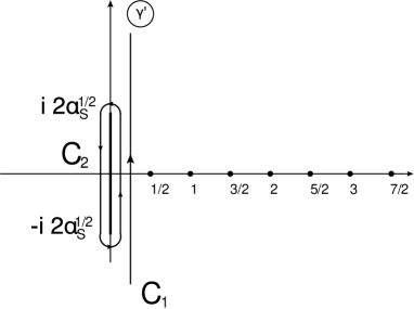
Fig. 1-a		Fig. 1-b

Figure 1: The $\gamma$ - plane: the contours of integrations over $\gamma^{\prime}$ in Eq. (21) and in Eq. (39) (Fig. 1-a); and the contours of integrations in general case (Fig. 1-b).

Hence the solution can be written in the form:

$$\tilde{N}\left(\tilde{\xi},Y\right)\,\,=\,\,\frac{1}{2\,\pi}\int_{C_{2}}\!\!\!\!d\gamma^{\prime}\,e^{i\,\gamma^{\prime}\left(\tilde{\xi}\,\,-\,\,\frac{1}{2}\,Y\right)}\,\phi_{in}(i\,\gamma^{\prime})\,\sum^{\infty}_{n=0}\frac{\left(\frac{1}{2}\sqrt{4\bar{\alpha}_{S}\,-\,\gamma^{\prime 2}}\,\,\,Y\right)^{2n\,+\,1}}{(2n\,+\,1)!}$$ (40)

For small values of $\bar{\alpha}_{S}$ we can safely replace $\gamma^{\prime}$ by $\gamma^{\prime}=0$ in $\phi_{in}\left(i\gamma^{\prime}\right)$ and take the integral, using formula 3.771(8) of Ref. RY :

$$\int^{2\sqrt{\bar{\alpha}_{S}}}_{-2\sqrt{\bar{\alpha}_{S}}}\!\!\!\!d\gamma^{\prime}\,e^{i\,\gamma^{\prime}\left(\tilde{\xi}\,\,-\,\,\frac{1}{2}\,Y\right)}\,\frac{\left(\frac{1}{2}\sqrt{4\bar{\alpha}_{S}\,-\,\gamma^{\prime 2}}\,\,\,Y\right)^{2n\,+\,1}}{(2n\,+\,1)!}\,\,=$$ (41)

$$\,\,=\,\phi_{in}\left(0\right)\,\,\displaystyle{2\,\sqrt{\pi}(2\,\alpha_{S})^{n+1}Y^{2n+1}\dfrac{\Gamma\left(n+\frac{3}{2}\right)}{\Gamma(2n+2)}J_{n+1}(\sqrt{\alpha_{S}}|2\,\tilde{\xi}-Y|)(\sqrt{\alpha_{S}}|2\,\tilde{\xi}-Y|)^{-(n+1)}}$$

$$\,\,=\,\,\phi_{in}\left(0\right)\,\,\displaystyle{\dfrac{2\sqrt{\alpha_{S}}\pi Y}{|2\,\tilde{\xi}-Y|}\dfrac{1}{n!}J_{n+1}(\sqrt{\alpha_{S}}|2\,\tilde{\xi}-Y|)\left(2\,\dfrac{(\sqrt{\alpha_{S}}Y/2)^{2}}{\sqrt{\alpha_{S}}|2\,\tilde{\xi}-Y|}\right)^{n}}$$

where we use the duplication formula of the Gamma function(see formula 8.335(1) of Ref.RY ): $\Gamma\left(2(n+1)\right)\,=\,\left(2^{2n+1}/\sqrt{\pi}\right)\Gamma\left(n+1\right)\,\Gamma\left(n+3/2\right)$.

Plugging Eq. (41) into Eq. (39) we obtain

$$N(\tilde{\xi},Y)\,\,\,=\,\,\,e^{-\tilde{\xi}}\,\,\phi_{in}\left(0\right)\,\,\dfrac{\sqrt{\bar{\alpha}_{S}}Y}{|2\,\tilde{\xi}-Y|}\displaystyle{\sum_{n=0}^{\infty}\dfrac{\tau^{n}}{n!}J_{n+1}(\sqrt{\bar{\alpha}_{S}}|\,2\,\tilde{\xi}-Y|)}$$ (42)

with $\tau\,\,=\,\,2\,(\sqrt{\alpha_{S}}\,\frac{1}{2}Y)^{2}/(\sqrt{\bar{\alpha}_{S}}|2\,\tilde{\xi}-Y|)$. For $|\tilde{\xi}-Y|^{2}>Y^{2}/2$ the series term can be summed using formula 5.7.6.1 in Ref.PR . Hence, we obtain the explicit form of the solution

$$N\left(\tilde{\xi},Y\right)\,\,\,=\,\,\,e^{-\tilde{\xi}}\,\,\phi_{in}\left(0\right)\,\,\displaystyle{\bar{\alpha}_{S}Y\dfrac{J_{1}\left(2\,\sqrt{\bar{\alpha}_{S}\,\tilde{\xi}\,\left(\tilde{\xi}-Y\right)}\right)}{\sqrt{\bar{\alpha}_{S}\,\tilde{\xi}\,\left(\tilde{\xi}-Y\right)}}}$$ (43)

In Fig. 2 we plot $\tilde{N}\left(\tilde{\xi},Y\right)$. For the LO BFKL equation this function increases with $\tilde{\xi}$. From Fig. 2 one can see that (i) at large $b$ the solution decreases as the power of $b$; (ii) in the limited range of $\xi$ we can parameterize this decrease as $\tilde{N}\propto\exp\left(-\mu^{2}b^{2}\right)$ with $\mu^{2}={\rm Const}/(rR)$ for sufficiently small values of ${\rm Const}$; and (iii) at large $b$ we have oscillating behaviour, which is in contradiction to $\tilde{N}\,>\,0$, that follows from the unitarity constraints.

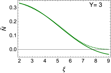
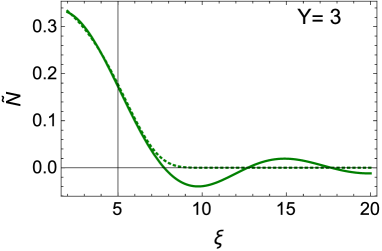
Fig. 2-a		Fig. 2-b
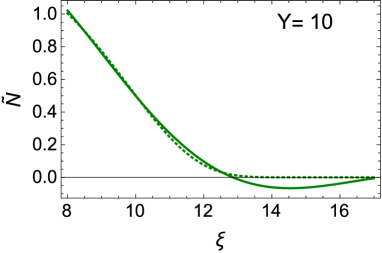
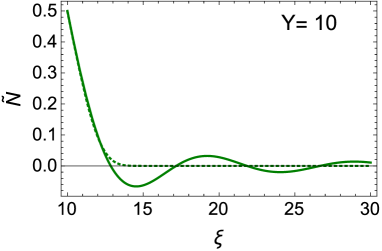
Fig. 2-c		Fig. 2-d

Figure 2: Solution $\tilde{N}\left(Y,\xi\right)$ of Eq. (43) versus $\xi$ (solid lines). The dotted lines are the fit $\tilde{N}\propto\exp\left(-\mu^{2}b^{2}\right)$ with $\mu^{2}=0.07/(rR)$ for Fig. 2-a and Fig. 2-b and $\mu^{2}\,=\,0.007/(rR)$ for Fig. 2-c and Fig. 2-d. In all estimates $\bar{\alpha}_{S}=0.2$.

All these features can be seen from the asymptotic behaviour of Eq. (43) at large $\xi\,\gg\,Y$. One can see that the scattering amplitude

$$N(\tilde{\xi},Y)\,\,\,\propto\,\,\,e^{-\tilde{\xi}}\frac{\cos\left(\frac{\pi}{4}-2\,\sqrt{\bar{\alpha}_{S}}\,\tilde{\xi}\,\right)}{\left(2\sqrt{\bar{\alpha}_{S}}\,\tilde{\xi}\right)^{3/2}}\,\,\leq\,\,\frac{r^{2}\,R^{2}}{b^{4}}$$ (44)

Therefore, we have power-like bahaviour of the scattering amplitude at large $b$, which leads to the violation of the Froissart theorem KW1 ; KW2 ; KW3 .

For $\tilde{\xi}\,<\,Y$ the solution takes the form

$$N\left(\tilde{\xi},Y\right)\,\,\,=\,\,e^{-\tilde{\xi}}\,\,\phi_{in}\left(0\right)\,\bar{\alpha}_{S}Y\,\left(\displaystyle{\dfrac{I_{1}\left(2\,\sqrt{\bar{\alpha}_{S}\,\tilde{\xi}\,\left(Y-\tilde{\xi}\right)}\right)}{\sqrt{\bar{\alpha}_{S}\,\tilde{\xi}\,\left(Y-\tilde{\xi}\right)}}}\right)$$ (45)

Therefore, the general solution can be written as

$$N\left(\tilde{\xi},Y\right)\,\,\,=$$ (46)

$$\,\,\,e^{-\tilde{\xi}}\,\,\phi_{in}\left(0\right)\,\bar{\alpha}_{S}Y\,\left(\displaystyle{\dfrac{I_{1}\left(2\,\sqrt{\bar{\alpha}_{S}\,\tilde{\xi}\,\left(Y-\tilde{\xi}\right)}\right)}{\sqrt{\bar{\alpha}_{S}\,\tilde{\xi}\,\left(Y-\tilde{\xi}\right)}}}\,\Theta\left(Y\,-\,\tilde{\xi}\right)\,\,+\,\,\displaystyle{\dfrac{J_{1}\left(2\,\sqrt{\bar{\alpha}_{S}\,\tilde{\xi}\,\left(\tilde{\xi}-Y\right)}\right)}{\sqrt{\bar{\alpha}_{S}\,\tilde{\xi}\,\left(\tilde{\xi}-Y\right)}}}\,\Theta\left(\tilde{\xi}\,-\,Y\right)\right)$$

This solution, is similar to the solution of the BFKL equation with time ordering (see Eq.(3.35) in Ref.DIMST ), if we replace $\tilde{\xi}$ by $\rho\,=\,\ln\left(R^{2}/r^{2}\right)$. We cannot claim that $\tilde{\xi}\,>\,Y$ corresponds to the unphysical kinematic region due to the time ordering, since the BFKL kernel does not depend on impact parameters.

IV.5 Numerical estimates

Summing over $n$ in Eq. (40) we can re-write the solution in the form:

$$\tilde{N}\left(\xi,Y\right)\,\,=\,\,\frac{1}{2\,\pi}\int^{2\sqrt{\bar{\alpha}_{S}}}_{-2\sqrt{\bar{\alpha}_{S}}}d\gamma^{\prime}\Bigg{(}e^{\frac{1}{2}\sqrt{4\bar{\alpha}_{S}\ -\,\gamma^{\prime 2}}\,Y}\,\,-\,\,e^{-\frac{1}{2}\sqrt{4\bar{\alpha}_{S}\ -\,\gamma^{\prime 2}}\,Y}\Bigg{)}\,\,e^{i\,\gamma^{\prime}\left(\xi\,\,-\,\,\frac{1}{2}\,Y\right)}\,\phi_{in}(i\,\gamma^{\prime})$$ (47)

In Fig. 3 we plot $N$, which comes from the numerical calculation for Eq. (47), choosing $B_{1}=\frac{1}{2}$ and $B_{2}=1$ in Eq. (13), taking $\bar{\alpha}_{S}=0.2$ and fixing $Y=10$. The logarithmic plot in this figure shows, first, that at large $b$ we have the power-like decrease, as we have discussed, and, second, that we can reproduce the solution which decreases as $e^{-1.06b/\sqrt{r\,R}}$ in the region of $\xi=4-10$. It should be stressed that such fast decrease cannot be achieved in the LO BFKL, for which, $\tilde{N}$ increases at large $b$. We will discuss this in detail in the conclusions below. It is interesting to note that the slope $1.06/\sqrt{r\,R}$ is close to one, that has been found in Ref.CCM for $r=R=10\,GeV^{-1}$.

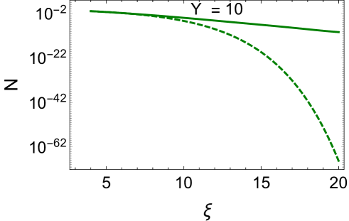
Figure 3: Numerical estimates for $N$, which comes from Eq. (47) fixing $B_{1}=\frac{1}{2}$ and $B_{2}=1$ in Eq. (13),$\bar{\alpha}_{S}=0.2$ and $Y=10$ (solid line) . The dotted line is $N\,\propto\,\exp\left(-1.06\,e^{\frac{1}{4}\xi}\right)$.

Tables I and II as well as Fig. 4 show that the slope $\mu$($N\,\propto\,e^{-\mu\,b}$) depend on the values of $Y$ and on the initial conditions. One can see that the range of $b$ in which we can trust the exponential parameterization also depends on the values of $r$ and $Y$, reproducing the main pattern of the solution given in Ref.CCM .

r ($GeV^{-1}$)	Y=10	Y=3
1	0.079	0.394
10	0.058	0.092
25	0.043	0.082
63	0.026	0.038

Table 1: Numerical value for the
slope $\mu$ in $GeV$ versus $Y=\ln(1/x)$

r ($GeV^{=1}$)	$B_{1}$=1/2,$B_{2}$ =1	$B_{1}$=1/2,$B_{2}$ =2	$B_{1}$=1/3,$B_{2}$ =1
1	0.079	0.067	0.076
10	0.058	0.053	0.057
25	0.043	0.036	0.039
63	0.026	0.023	0.022

Table 2: Numerical value for the slope $\mu$ in $GeV$ for $Y=10$ and for different values of $B_{1}$ and $B_{2}$.

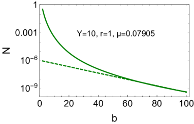
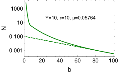
Fig. 4-a		Fig. 4-b
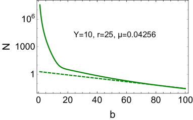
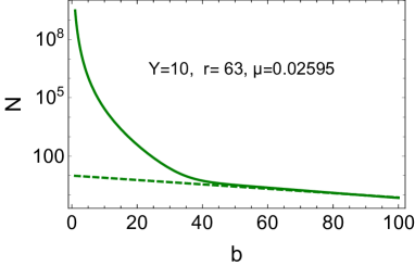
Fig. 4-c		Fig. 4-d

Figure 4: Numerical estimates of Eq. (47) for different values of $r=R$ at $Y=\ln(1/x)$ = 10 (solid lines). The dotted lines denote $N\propto\exp\left(-\mu b\right)$. The slope $\mu$ is in $GeV$, while $r$ and $b$ are in $GeV^{-1}$. For all estimates $\bar{\alpha}_{S}=0.2$.

V Beyond DLA

In this section we modify the solution taking into account more complicated expressions for the eigenvalues than Eq. (20) and Eq. (23). We consider Eq. (9) and the eigenvalues $\omega\left(\bar{\alpha}_{S},\gamma\right)$ take the form

$$\omega\left(\bar{\alpha}_{S},\gamma\right)\,\,=$$ (48)

$$\,\,\underbrace{\frac{-\bar{\alpha}_{S}+\gamma-1+\bar{\alpha}_{S}\gamma\Phi(\gamma)}{2(\alpha\Phi(\gamma)+1)}}_{\omega^{\prime}\left(\bar{\alpha}_{S},\gamma\right)}\,+\,\underbrace{\frac{\sqrt{(\bar{\alpha}_{S}(-\gamma)\Phi(\gamma)+\bar{\alpha}_{S}-\gamma+1)^{2}-4(\bar{\alpha}_{S}\Phi(\gamma)+1)(\bar{\alpha}_{S}\gamma\Phi(\gamma)-\bar{\alpha}_{S}\Phi(\gamma)-\bar{\alpha}_{S})}}{2(\alpha\Phi(\gamma)+1)}}_{\omega^{\prime\prime}\left(\bar{\alpha}_{S},\gamma\right)}$$

with

$$\Phi(\gamma)\,\,=\,\,\frac{1}{\gamma}\,+\,2\psi(1)-\psi\left(2-\gamma\right)-\psi\left(1+\gamma\right)$$ (49)

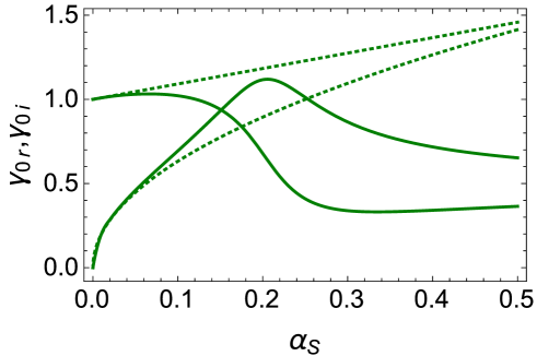
Figure 5: $\gamma_{0r}$(solid line) and $\gamma_{0i}$( dotted line) versus $\bar{\alpha}_{S}$. The roots for the DLA approach (see Eq. (23)) are shown by the dotted lines. In this case $\gamma_{0r}=1+\bar{\alpha}_{S}$ and $\gamma_{0i}\,=\,2\bar{\alpha}_{S}^{1/2}$

The singularities of $\omega\left(\bar{\alpha}_{S},\gamma\right)$ are related to the poles of $\Phi\left(\gamma\right)$, the zeroes of $1+\bar{\alpha}_{S}\Phi\left(\gamma\right)=0$ and $\omega"\left(\bar{\alpha}_{S},\gamma\right)$ has a branch point when the radicand is equal to zero. Near the zero of the radicand $\omega"\left(\bar{\alpha}_{S},\gamma\right)$ takes the form

$$\omega"\left(\bar{\alpha}_{S},\gamma\right)\,\,=\,\,A\left(\bar{\alpha}_{S}\right)\sqrt{\left(\gamma\,\,-\,\,\gamma_{0r}\right)^{2}\,+\,\gamma^{2}_{0i}}$$ (50)

Eq. (50) has two complex roots: $\gamma\,\,=\,\,\gamma_{0r}\,\,\pm\,\,i\,\gamma_{0i}$. In Fig. 5 we plot $\gamma_{0r}$ and $\gamma_{0i}$ as functions of $\bar{\alpha}_{S}$. From this figure shows that for very small values of $\bar{\alpha}_{S}$ our solution coincides with the DLA approximation. However, for $\bar{\alpha}_{S}\,>\,0.05$ the values of $\gamma_{0r}$ and $\gamma_{0i}$ differ considerably from their DLA values, approaching their maxima at large $\bar{\alpha}_{S}$.

The contours of the integration over $\gamma^{\prime}=1-\gamma$ are shown in Fig. 1-b. The integration over contour $C_{2}$ in Fig. 1-b can be written in the form

$$\tilde{N}\left(\xi,Y\right)\,\, = \,\,\frac{1}{2\,\pi}\int^{\gamma_{0i}}_{-\gamma_{0i}}\,d\gamma^{\prime\prime}\exp\left(\omega^{\prime}\left(\bar{\alpha}_{S},\gamma=\gamma_{0r}\right)\,Y\,+\,i\,\frac{d\omega^{\prime}\left(\bar{\alpha}_{S},\gamma=\gamma_{0r}\right)}{d\gamma}\gamma^{\prime\prime}\,Y\,+\,i\gamma^{\prime\prime}\,\xi\right)$$ (51)

$$\times \,\,\left(\exp\left(A\left(\bar{\alpha}_{S}\right)\,Y\,\sqrt{\gamma^{2}_{0i}\,\,-\,\,\gamma^{\prime\prime 2}}\right)\,\,-\,\,\exp\left(-A\left(\bar{\alpha}_{S}\right)\,Y\,\sqrt{\gamma^{2}_{0i}\,\,-\,\,\gamma^{\prime\prime 2}}\right)\right)$$

Introducing the new notation: $\omega_{0}\left(\bar{\alpha}_{S}\right)\,=\,\omega^{\prime}\left(\bar{\alpha}_{S},\gamma=\gamma_{0r}\right)$ and $B\left(\bar{\alpha}_{S}\right)\,=\,\frac{d\omega^{\prime}\left(\bar{\alpha}_{S},\gamma=\gamma_{0r}\right)}{d\gamma}$ we can evaluate the integral of Eq. (51) using the same procedure, as we have discussed in section IV-D, or using formula 3.711 of Ref.RY continuing it analytically for imaginary $A$.

Finally,

$$\tilde{N}\left(\xi,Y\right)\,\,=\,\,Y\,\gamma_{0i}\,A\left(\bar{\alpha}_{S}\right)e^{\omega_{0}\left(\bar{\alpha}_{S}\right)Y}\frac{J_{1}\left(\gamma_{0,i}\sqrt{\left(\xi+B\left(\bar{\alpha}_{S}\right)Y\right)^{2}\,\,-\,\,A^{2}\left(\bar{\alpha}_{S}\right)Y^{2}}\right)}{\sqrt{\left(\xi+B\left(\bar{\alpha}_{S}\right)Y\right)^{2}\,\,-\,\,A^{2}\left(\bar{\alpha}_{S}\right)Y^{2}}}$$ (52)

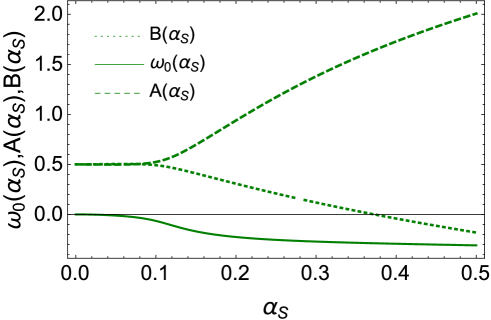
Figure 6: $\omega_{0}\left(\bar{\alpha}_{S}\right),A\left(\bar{\alpha}_{S}\right),B\left(\bar{\alpha}_{S}\right)$ versus $\bar{\alpha}_{S}$.

The $\bar{\alpha}_{S}$ dependence of all parameters in Eq. (52) are shown in Fig. 6.

In Fig. 7 we give several examples of the behaviour of $\tilde{N}$ in different kinematic regions. One can see that in spite of numerical differences, the claim that $\xi\,<\,Y$ give the main contribution is correct.

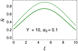
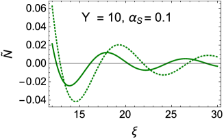
Fig. 7-a		Fig. 7-b
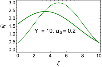
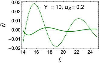
Fig. 7-c		Fig. 7-d
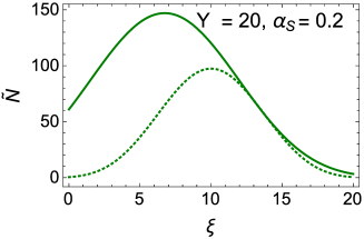
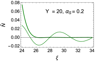
Fig. 7-e		Fig. 7-f

Figure 7: Solutions of Eq. (52) (solid lines) and solution of Eq. (46) (dotted lines) in different kinematic regions.

VI Conclusions

In this paper, we show that the NLO corrections do not change the power-like decrease of the scattering amplitude at large impact parameter and, therefore, they cannot resolve the contradiction with the unitarityKW1 ; KW2 ; KW3 . On the other hand, in a limited range of $b$, the NLO corrections lead to a fast decrease of the scattering amplitude with $b$, which can be parameterized as $N\,\propto\,\exp\left(-\,\mu^{2}\,b^{2}\right)$ with $\mu^{2}\propto 1/r^{2}$, in accord with the numerical estimates in Ref.CCM .

We demonstrate that the NLO correction leads to an oscillating behaviour of the scattering amplitude as function of $b$. Such oscillations contradict the unitarity constraints, as $N$, being the imaginary part of the scattering amplitude, should be positive ($N\,>\,0$).

However, from the more practical point of view, the NLO estimates give the faster decrease of the scattering amplitude as a function of $b$ (see Fig. 8) and could be useful in the description of the experimental data (see Ref.CCM ).

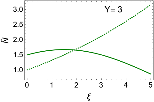
Figure 8: Comparison of the NLO calculation(solid line) with the LO estimates (dotted line).$\bar{\alpha}_{S}$ = 0.2. Y = 3.

In a sense, we showed that the scattering amplitude is negligibly small at $\tilde{\xi}\,>\,Y$( $b^{2}>r^{2}\,\exp\left(\frac{1}{2}\,\eta\right)$). The violation of the Froissart theorem stems from the smaller values of $\xi$. Indeed, for $\xi\,<\,Y$ the scattering amplitude is proportional to $N\,\propto\,\exp\left(2\sqrt{\bar{\alpha}_{S}\,\xi\,\left(Y\,-\,\xi\right)}\,-\,\xi\right)$ (see Eq. (46)) and $N\ll\,1$ for $\xi\,\geq\,4\bar{\alpha}_{S}Y/(1+4\,\bar{\alpha}_{S})$. Choosing $\xi_{0}=\ln\left(b^{2}_{0}/r^{2}\right)$ we see that

$$\sigma\,=\,2\,\int d^{2}bN\,\,\leq\,\,2\pi\int^{b^{2}_{0}}d\,b^{2}\,\,\sim\,\,b^{2}_{0}\,=\,r^{2}e^{4\bar{\alpha}_{S}\eta/(1+4\,\bar{\alpha}_{S})}\,\gg\,Y^{2}$$ (53)

Therefore, the range of $b^{2}\,<\,r^{2}\,e^{4\bar{\alpha}_{S}\eta/(1+4\,\bar{\alpha}_{S})}$ turns out to be wide enough to violate the Froissart theoremKW1 ; KW2 ; KW3 . Hence, the resumed NLO kernel cannot heal the problem of violation of the Froissart theorem and has an additional defect of the oscillating behaviour at $\xi>Y$, which is in contradiction to the unitarity constraints, which lead to $N>0$.

We believe that we need to introduce non-perturbative corrections with an additional dimensional scale to the BFKL kernel, and that their influence will be much more important than that of the NLO BFKL kernel that we have discussed here.

VII Acknowledgements

We thank our colleagues at Tel Aviv university and UTFSM for the discussions. The special thanks go to Asher Gotsman his encouraging support. This research was supported by Proyecto Basal FB 0821(Chile), Fondecyt (Chile) grants 1180118 and 1191434.

References

- (1) J. Cepila, J. G. Contreras and M. Matas, Phys. Rev. D 99 (2019) no.5, 051502 doi:10.1103/PhysRevD.99.051502 [arXiv:1812.02548 [hep-ph]].
- (2) Yuri V Kovchegov and Eugene Levin, “ Quantum Choromodynamics at High Energies", Cambridge Monographs on Particle Physics, Nuclear Physics and Cosmology, Cambridge University Press, 2012 .
- (3) A. Kovner and U. A. Wiedemann, Phys. Rev. D 66, 051502 (2002) [hep-ph/0112140].
- (4) A. Kovner and U. A. Wiedemann, Phys. Rev. D 66, 034031 (2002) [hep-ph/0204277].
- (5) A. Kovner and U. A. Wiedemann, Phys. Lett. B 551, 311 (2003) [hep-ph/0207335].
-
(6)
M. Froissart,
Phys. Rev. 123 (1961) 1053;
A. Martin, “Scattering Theory: Unitarity, Analitysity and Crossing." Lecture Notes in Physics, Springer-Verlag, Berlin-Heidelberg-New-York, 1969. - (7) E. M. Levin and M. G. Ryskin, Sov. J. Nucl. Phys. 50, 881 (1989) [Z. Phys. C 48, 231 (1990)] [Yad. Fiz. 50, 1417 (1989)].
- (8) K. J. Golec-Biernat and A. M. Stasto, Nucl. Phys. B 668, 345 (2003) [hep-ph/0306279].
- (9) E. Gotsman, M. Kozlov, E. Levin, U. Maor and E. Naftali, Nucl. Phys. A 742, 55 (2004) [hep-ph/0401021].
- (10) J. Berger and A. M. Stasto, Phys. Rev. D 84 (2011) 094022 doi:10.1103/PhysRevD.84.094022 [arXiv:1106.5740 [hep-ph]].
- (11) J. Berger and A. Stasto, Phys. Rev. D 83, 034015 (2011) [arXiv:1010.0671 [hep-ph]].
- (12) J. Berger and A. M. Stasto, JHEP 1301 (2013) 001 doi:10.1007/JHEP01(2013)001 [arXiv:1205.2037 [hep-ph]].
- (13) E. Levin and S. Tapia, JHEP 1307, 183 (2013) doi:10.1007/JHEP07(2013)183 [arXiv:1304.8022 [hep-ph]].
- (14) E. Levin, L. Lipatov and M. Siddikov, Phys. Rev. D 89 (2014) no.7, 074002 doi:10.1103/PhysRevD.89.074002 [arXiv:1401.4671 [hep-ph]].
- (15) E. Levin, Phys. Rev. D 91 (2015) no.5, 054007 [arXiv:1412.0893 [hep-ph]].
- (16) V. S. Fadin, E. A. Kuraev and L. N. Lipatov, Phys. Lett. B60, 50 (1975); E. A. Kuraev, L. N. Lipatov and V. S. Fadin, Sov. Phys. JETP 45, 199 (1977), [Zh. Eksp. Teor. Fiz.72,377(1977)]; I. I. Balitsky and L. N. Lipatov, Sov. J. Nucl. Phys. 28, 822 (1978), [Yad. Fiz.28,1597(1978)].
- (17) L. N. Lipatov, “Small x physics in perturbative QCD,” Phys. Rept. 286, 131 (1997) [hep-ph/9610276]; “The Bare Pomeron in Quantum Chromodynamics,” Sov. Phys. JETP 63, 904 (1986) [Zh. Eksp. Teor. Fiz. 90, 1536 (1986)].
- (18) V. S. Fadin and L. N. Lipatov, Phys. Lett. B 429 (1998) 127 [hep-ph/9802290].
- (19) M. Ciafaloni and G. Camici, Phys. Lett. B 430 (1998) 349 [hep-ph/9803389].
- (20) G. P. Salam, JHEP 9807 (1998) 019 doi:10.1088/1126-6708/1998/07/019 [hep-ph/9806482];
- (21) M. Ciafaloni, D. Colferai and G. P. Salam, Phys. Rev. D 60 (1999) 114036 doi:10.1103/PhysRevD.60.114036 [hep-ph/9905566].
- (22) M. Ciafaloni, D. Colferai, G. P. Salam and A. M. Stasto, Phys. Rev. D 68 (2003) 114003, [hep-ph/0307188].
- (23) V. A. Khoze, A. D. Martin, M. G. Ryskin and W. J. Stirling, Phys. Rev. D 70 (2004) 074013 [hep-ph/0406135].
- (24) B. Duclou? E. Iancu, A. H. Mueller, G. Soyez and D. N. Triantafyllopoulos, JHEP 1904 (2019) 081 doi:10.1007/JHEP04(2019)081 [arXiv:1902.06637 [hep-ph]].
- (25) M. Abramowitz and I. Stegun. Handbook of mathematical functions: with formulas, graphs, and mathematical tables. Courier Dover Publications, 1972.
- (26) I. Gradstein and I. Ryzhik, Table of Integrals, Series, and Products, Fifth Edition, Academic Press, London, 1994
- (27) A.P.Prudnikov, Yu. A. Brychkov, and O.I. Marichev. Integrals and Series, vol.2. Special functions, Gordon and Breach, New York, 1992.