Distributed, Egocentric Representations of Graphs for
Detecting Critical Structures

Distributed, Egocentric Representations of Graphs for Detecting Critical Structures: Supplementary Metarials

Abstract

We study the problem of detecting critical structures using a graph embedding model. Existing graph embedding models lack the ability to precisely detect critical structures that are specific to a task at the global scale. In this paper, we propose a novel graph embedding model, called the Ego-CNNs, that employs the ego-convolutions convolutions at each layer and stacks up layers using an ego-centric way to detects precise critical structures efficiently. An Ego-CNN can be jointly trained with a task model and help explain/discover knowledge for the task. We conduct extensive experiments and the results show that Ego-CNNs (1) can lead to comparable task performance as the state-of-the-art graph embedding models, (2) works nicely with CNN visualization techniques to illustrate the detected structures, and (3) is efficient and can incorporate with scale-free priors, which commonly occurs in social network datasets, to further improve the training efficiency.

1 Introduction

A graph embedding algorithm converts graphs from structural representation to fixed-dimensional vectors. It is typically trained in a unsupervised manner for general learning tasks but recently, deep learning approaches (Bruna et al., 2013; Kipf & Welling, 2017; Atwood & Towsley, 2016; Duvenaud et al., 2015; Li et al., 2016; Pham et al., 2017; Gilmer et al., 2017; Niepert et al., 2016) are trained in a supervised manner and show superior results against unsupervised approaches on many tasks such as node classification and graph classification.

While these algorithms lead to good performance on tasks, what valuable information can be jointly learned from the graph embedding is less discussed. In this paper, we aim to develop a graph embedding model that jointly discovers the critical structures, i.e., partial graphs that are dominant to a prediction in the task (e.g., graph classification) where the embedding is applied to. This helps people running the task understand the reason behind the task predictions, and is particularly useful in certain domains such as the bioinformatics, cheminformatics, and social network analysis, where valuable knowledge may be discovered by investigating the found critical structures.

(a)	(b)

Figure 1: (a) The OH function group is the critical structure to tell Alcohols from Alkanes. (b) The symmetry hydrocarbon group (at two sides of the methyl branch) is the critical structure to discriminate between symmetric and asymmetric isomer of methylnonane.

However, identifying critical structures is a challenging task. The first challenge is that critical structures are task-specific—the shape and location of critical structures may vary from task to task. This means that the graph embedding model should be learned together with the task model (e.g., a classifier or regressor). The second challenge is that model needs to be able to detect precise critical structures. For example, to discriminant Alcohols from Alkanes (Figure 1(a)), one should check if there exists an OH-base and if the OH-base is at the end of the compound. To be helpful, a model has to identify the exact OH-base rather than its approximation in any form. Third, the critical structures need to be found at the global-scale. For example, in the task aiming to identify if a methyl-nonane is symmetric or not (Figure 1(b)), one must check the entire graph to know if the methyl is branched at the center position of the long carbon chain. In this task, the critical structure is the symmetric hydrocarbon at the two sides of the methyl branch, which can only be found at the global-scale. Unfortunately, finding out all matches of substructures in a graph is known as subgraph isomorphism and proven to be an NP-complete problem (Cook, 1971). To the best of our knowledge, there is no existing graph embedding algorithm that can identify task-dependent, precise critical structures up to the global-scale in an efficient manner.

Table 1: A comparison of embedding models for a graph $\mathcal{G}=(\mathcal{V},\mathcal{E})$, $|\mathcal{V}|=N$, where $D$ is the embedding dimension, $K$ is the maximum node degree in $\mathcal{G}$, $L$ is the number of layers of a deep model, and $C$ is a graph-specific constant.

Graph embedding model	Task-Specific?	Precise critical structures?	Exponential scale efficiency?	Efficient on large graphs?	Time complexity (forward pass)
WL kernel (Shervashidze et al., 2011)			✓	✓	$O(L(KN+C))$
DGK (Yanardag & Vishwanathan, 2015)				✓	$O(DCN)$
Subgraph2vec (Narayanan et al., 2016)				✓	$O(DCN)$
MLG (Kondor & Pan, 2016)			✓		$O(LN^{5})$
Structure2vec (Dai et al., 2016)	✓		✓	✓	$O((KD+D^{2})LN)$
Spatial GCN (Bruna et al., 2013)	✓	✓			$O(DLN^{2})$
Spectrum GCN (Bruna et al., 2013; Defferrard et al., 2016; Kipf & Welling, 2017)	✓		✓	✓	$O(D^{2}L|\mathcal{E}|)$
DCNN (Atwood & Towsley, 2016)	✓				$O(MDN^{2})$
Patchy-San (Niepert et al., 2016)	✓	✓		✓	$O(K^{2}DN)$
Message-Passing NNs (Duvenaud et al., 2015; Li et al., 2016; Pham et al., 2017; Gilmer et al., 2017; Velickovic et al., 2018; Ying et al., 2018)	✓		✓	✓	$O(K^{2}D^{2}LN)$
Ego-CNN	✓	✓	✓	✓	$O(KD^{2}LN)$

In this paper, we present the Ego-CNNs that embed a graph into distributed (multi-layer), fixed-dimensional tensors. An Ego-CNN is a feedforward convolutional neural network that can be jointly learned with a supervised task model (e.g., fully-connected layers) to help identify the task-specific critical structures. The Ego-CNNs employ novel ego-convolutions to learn the latent representations at each network layer. Unlike the neurons in most existing task-specific, NN-based graph embedding models (Bruna et al., 2013; Kipf & Welling, 2017; Atwood & Towsley, 2016; Duvenaud et al., 2015; Li et al., 2016; Pham et al., 2017; Gilmer et al., 2017) which detect only fuzzy patterns, a neuron in an Ego-CNN can detect precise patterns in the output of the previous layer. This allows the precise critical structures to be backtracked following the model weights layer-by-layer after training. Furthermore, we propose the ego-centric design for stacking up layers, where the receptive fields of neurons across layers center around the same nodes. Such design avoids the locality and efficiency problems in existing precise model (Niepert et al., 2016) and enables efficient detection of critical structures at the global scale.

We conduct extensive experiments and the results show that Ego-CNNs work nicely with some common visualization techniques for CNNs, e.g., Transposed Deconvolution (Zeiler et al., 2011), can successfully output critical structures behind each prediction made by the jointly trained task model, and in the meanwhile, achieving performance comparable to the state-of-the-art graph classification models. We also show that Ego-CNNs can readily incorporate the scale-free prior, which commonly exists in large (social) graphs, to further improve the training efficiency in practice. To the best of our knowledge, the Ego-CNNs are the first graph embedding model that can efficiently detect task-dependent, precise critical structures at the global scale.

2 Related Work

Next, we briefly review existing graph embedding models. Table 1 compares the Ego-CNNs with existing graph embedding approaches. For an in-depth review of existing work, please refer to Section 1 of the supplementary materials or the survey (Cai et al., 2018).

Traditional graph kernels, including the Weisfeiler-Lehman (WL) kernel (Shervashidze et al., 2011), Deep Graph Kernels (DGKs) (Yanardag & Vishwanathan, 2015), Subgraph2vec (Narayanan et al., 2016), and Multiscale Laplacian Graph (MLG) Kernels (Kondor & Pan, 2016) are designed for unsupervised tasks. They have difficulty of finding task-specific critical structures.

Some recent studies aim to learn the task-specific graph embeddings. Structure2vec (Dai et al., 2016) uses approximated inference techniques to embed a graph. Studies, including Spectrum Graph Convolutional Network (GCN) (Bruna et al., 2013) and its variant (Kipf & Welling, 2017), Diffusion Convolutional Neural Networks (DCNNs) (Atwood & Towsley, 2016), and Message-Passing Neural Networks (MPNNs) (Duvenaud et al., 2015; Li et al., 2016; Pham et al., 2017; Gilmer et al., 2017; Velickovic et al., 2018; Ying et al., 2018), borrow the concepts of CNNs to embed graphs. The idea is to model the filters/kernels that scan through different parts of the graph (which we call the neighborhoods) to learn patterns most helpful to the learning task. However, the above work share a drawback that they can only identify fuzzy critical structures or critical structures of very simple shapes due to the ways the convolutions are defined (to be elaborated later in this secion). Recently, a node embedding model, called the Graph Attention Networks (GATs) (Velickovic et al., 2018), is proposed. The GAT attention can be 1- or multi-headed. The multi-head-attention GATs aggregate hidden representations just like Message-Passing NNs and thus cannot detect precise critical structures. On the other hand, the 1-head-attention GATs allow backtracking precise nodes covered by a neuron through their masked self-attentional layers. However, being node embedding models, the 1-head-attention GATs can only detect simplified patterns in neighborhoods. The Ego-CNNs are a generalization of 1-head-attention GATs for graph embedding. We will compare these two models in more details in Section 3.1.

The only graph embedding models that allow backtracking nodes covered by a neuron are Spatial GCN (Bruna et al., 2013) and Patchy-San (Niepert et al., 2016). Unfortunately, the Spatial GCN is not applicable to our problem since it aims to perform hierarchical clustering of nodes. The filters learn the distance between clusters (a graph-level information) rather than subgraph patterns. On the other hand, the Patchy-San (Niepert et al., 2016) can detect precise critical structures. However, it is a single-layer NN designed to detect only the local critical structures around each node. Due to the lack of recursive definition of convolutions at deep layers, the Patchy-San does not enjoy the exponential efficiency of detecting large-scale critical structures using multiple layers as in other CNN-based models.

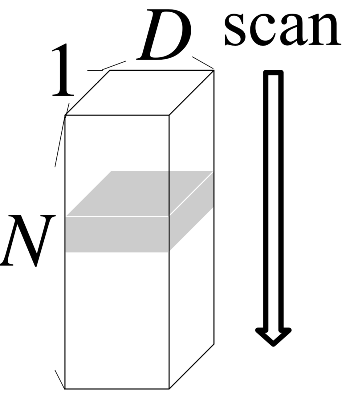
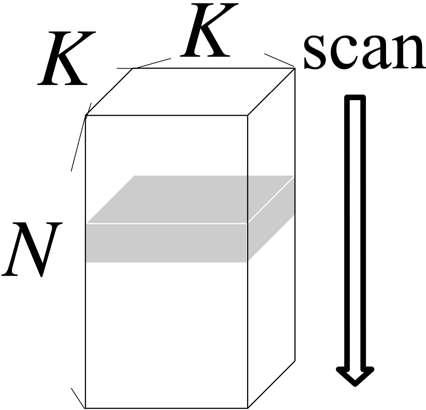
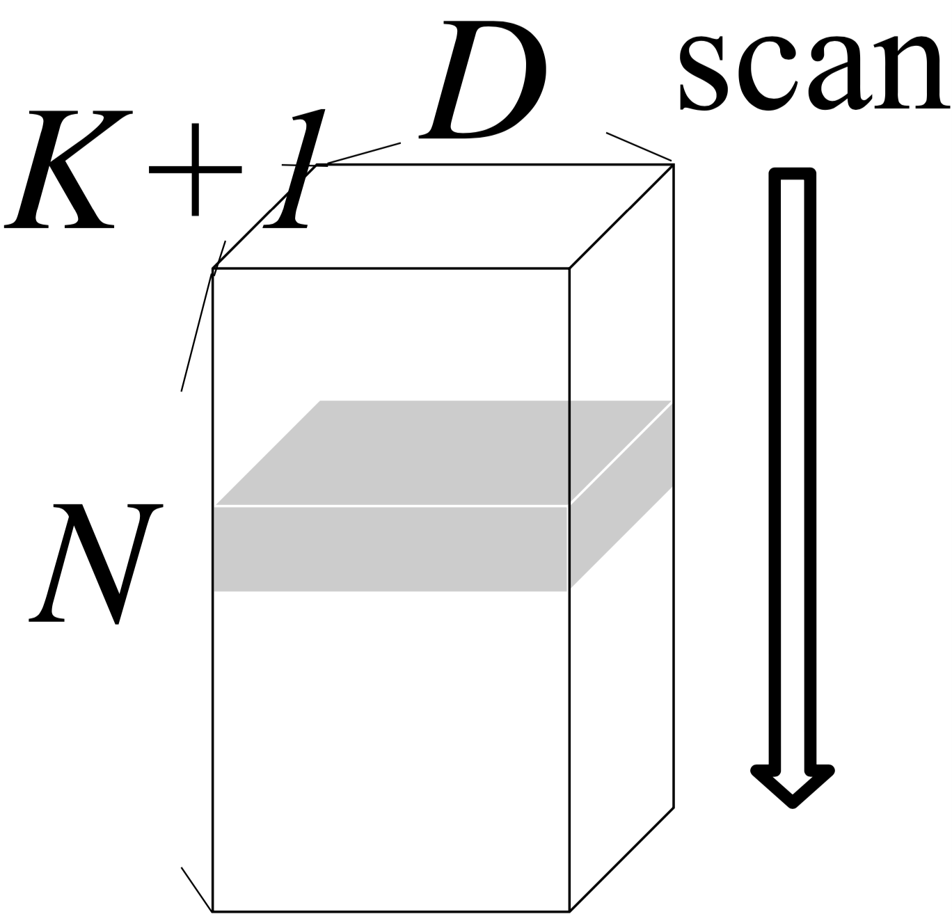
(a)	(b)	(c)

Figure 2: Neighborhood of a node $n$ in (a) Message-Passing NNs (Duvenaud et al., 2015; Li et al., 2016; Pham et al., 2017; Gilmer et al., 2017): $\boldsymbol{g}_{n}^{(l)}\in\mathbb{R}^{D}$ the aggregated hidden representations of adjacent nodes in the previous layer; (b) Patchy-San (Niepert et al., 2016): $\boldsymbol{A}^{(n)}\in\mathbb{R}^{K\times K}$ the adjacency matrix of $K$ nearest neighbors of node $n$, and (c) Ego-CNNs: ${\displaystyle\boldsymbol{E}^{(n,l)}}\in\mathbb{R}^{(K+1)\times D}$ the hidden representation of the $l$-hop ego network centered at node $n$ with $K$ nearest neighbors.

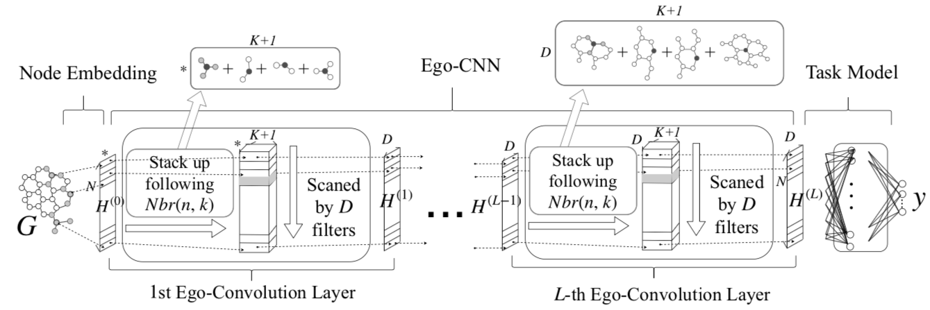
Figure 3: The model architecture of an Ego-CNN. With our egocentric design, neighborhoods are egocentrically enlarged by 1-hop after each Ego-Convolution layer. The dashed horizontal lines across layers indicate neighborhoods of the same node; the ? mark indicates an arbitrary dimension.

Neighborhoods. To understand the cause of limitations in existing work, we look into the definitions of neighborhoods in these models, as shown in Figure 8. In a CNN, a filters/kernel scans through different neighborhoods in a graph to detect the repeating patterns across neighborhoods. Hence, the definition of a neighborhood determines what to be learned by the model. In Message-Passing NNs (Duvenaud et al., 2015; Li et al., 2016; Pham et al., 2017; Gilmer et al., 2017) (Figure 8(a)), the $d$-th filter $\boldsymbol{w}^{(l,d)}\in\mathbb{R}^{D}$, $d=1,2,\cdots,D$, at the $l$-th layer scans through the $D$-dimensional vector $\boldsymbol{g}^{(n,l)}$ of every node $n$. The vector $\boldsymbol{g}^{(n,l)}=\bigoplus_{m\in Adj(n)}\boldsymbol{h}^{(m,l-1)}\in\mathbb{R}^{D}$ is an aggregation $\bigoplus$ (e.g., summation (Duvenaud et al., 2015)) of the hidden representations $\boldsymbol{h}^{(m,l-1)}$’s of the adjacent nodes $m$’s at the $(l-1)$-th layer. The $d$-th dimension of the hidden representations $h_{d}^{(n,l)}$ of a node $n$ at the $l$-th layer is calculated by

$$h_{d}^{(n,l)}=\sigma(\boldsymbol{g}^{(n,l)\top}\boldsymbol{w}^{(l,d)}+b_{d}),$$ (1)

where $\sigma$ is an activation function and $b_{d}$ is a bias term. By stacking up layers in these models, a deep layer can efficiently detect patterns that cover exponentially more nodes than the patterns found in the shallow layers. However, these models loses the ability of detecting precise critical structures since the network weights $\boldsymbol{w}^{(l,d)}$’s at the $l$-th layer parametrize only the aggregated representations from the previous layer. It is hard (if not impossible) for these networks to backtrack the critical nodes in the $(l-1)$-th layer via the weights $\boldsymbol{w}^{(l,d)}$’s after model training.

The single-layer Patchy-San (Niepert et al., 2016) uses filters to detects patterns in the adjacency matrix of the $K$ nearest neighbors of each node. The neighborhood of a node $n$ is defined as the $K\times K$ adjacency matrix $\boldsymbol{A}^{(n)}$ of the $K$ nearest neighbors of the node (Figure 8(b)). Filters $\boldsymbol{W}^{(d)}\in\mathbb{R}^{K\times K}$, $d=1,2,\cdots,D$, scan through the adjacency matrix of each node to generate the graph embedding $\boldsymbol{H}\in\mathbb{R}^{N\times D}$, where

$${\displaystyle H_{n,d}=\sigma(\boldsymbol{A}^{(n)}\varoast\boldsymbol{W}^{(d)}+b_{d}})$$ (2)

is the output of an activation function $\sigma$, $b_{d}$ is the bias term, and $\varoast$ is the Frobenius inner product defined as $\boldsymbol{X}\varoast\boldsymbol{Y}={\displaystyle\varSigma_{i,j}X_{i,j}Y_{i,j}}$. Unlike in Message-Passing NNs, the filters $\boldsymbol{W}^{(d)}$’s in Patchy-San parametrize the non-aggregated representations of nodes. Thus, by backtracking the nodes via $\boldsymbol{W}^{(d)}$’s, one can discover precise critical structures. However, to detect critical structures at the global scale, each $\boldsymbol{A}^{(n)}$ needs to have the size of $N\times N$, making the filters $\boldsymbol{W}^{(d)}\in\mathbb{R}^{N\times N}$ hard to learn. Efficient detection of task-specific, precise critical structures at global scale remains an important but unsolved problem.

3 Ego-CNN

A deep CNN model, when applied to images, offers two advantages: (1) filers/kernels at a layer, by scanning the neighborhood of every pixel, detect location independent patterns, and (2) with a proper recursive definition of neighborhoods, a filter at a deep layer can reuse the output of neurons at the previous layer to efficiently detect patterns in pixel areas, called receptive fields, that are exponentially larger (in number of pixels) than those in a shallow layer, thereby overcoming the curse of dimensionality. We aim to keep these advantages on graphs when designing a CNN-based graph embedding model.

Since Patchy-San (Niepert et al., 2016) can detect precise critical structures at the local scale, it seems plausible to extend the notion of its neighborhoods to deep layers. In Patchy-San, the neighborhood of a node $n$ at the input (shallowest) layer is defined as the $K\times K$ adjacency matrix $\boldsymbol{A}^{(n)}$ of the $K$ nearest neighbors of the node. We can recursively define the neighborhood of the node $n$ at a deep layer $l$ as the $K\times K$ adjacency matrix $\boldsymbol{A}^{(n,l)}$ of the $K$ nearest neighbors having the most similar latent representations output from the previous layer $(l-1$).

However, this naive extension suffers from two drawbacks. First, the neighborhood is dynamic since the $K$ nearest neighbors may change during the training time. This prevents the filters from learning the location independent patterns. Second, as the neighborhoods at layer $(l-1)$ are dynamic, it is hard for a model designer to decide which neuron output at layer $(l-1)$ to wire up to a filter at layer $l$ such that the filter can reuse the output to exponentially increase the learning efficiency in detecting large-scale patterns. As we can see, the root cause of the above problems is the ill-defined neighborhoods. This motivate us to rethink the definition of neighborhoods from scratch.

3.1 Model Design

We propose the Ego-CNN model that (1) defines ego-convolutions at each layer where a filter at layer $l$ scans the neighborhood representing the $l$-hop ego network centered at every node, and (2) stacks up layers using an ego-centric way such that the neighborhoods of a node $n$ at layers $1,2,\cdots,L$ center around the same node, as shown in Figure 3.

Ego-Convolutions. Let $Nbr(n,k)$ be the $k$-th nearest neighbor of a node $n$ in the graph $\mathcal{G}$ and $\boldsymbol{H}^{(l)}\in\mathbb{R}^{N\times D}$ be the graph embedding output by $D$ filters $\boldsymbol{W}^{(l,1)},\cdots,\boldsymbol{W}^{(l,D)}$ at the $l$-th layer. For $l=1,\cdots,L$, we define

$$\begin{array}[]{c}{\displaystyle H_{n,d}^{(l)}=\sigma\left(\boldsymbol{E}^{(n,l)}\varoast\boldsymbol{W}^{(l,d)}+b_{d}^{(l)}\right)\text{, where }}\\ {\displaystyle\boldsymbol{E}^{(n,l)}=\left[\boldsymbol{H}_{n,:}^{(l-1)},\boldsymbol{H}_{Nbr(n,1),:}^{(l-1)},\cdots,\boldsymbol{H}_{Nbr(n,K),:}^{(l-1)}\right]^{\top}}\end{array}$$ (3)

The $\boldsymbol{E}^{(n,l)}\in\mathbb{R}^{(K+1)\times D}$ is a matrix representing the neighborhood of the node $n$ at the $l$-th layer, $\sigma$ is the activation function, $b_{d}$ is the bias term, and $\varoast$ is the Frobenius inner product defined as $\boldsymbol{X}\varoast\boldsymbol{Y}={\displaystyle\varSigma_{i,j}X_{i,j}Y_{i,j}}$. We determine the $K$ nearest neighbors of a node $n$ using the edge weights (if available) or hop count (otherwise), and define $\boldsymbol{H}_{n,:}^{(0)}\text{$\in\mathbb{R}$}^{K}$ as the adjacency vector between $n$ and its $K$ nearest neighbors. The goal of the model is to learn the filters (Figure 8(c)) and bias terms at all layers that minimize the loss defined by a task.

The neighborhood of a node $n$ at the $l$-th layer is recursively defined as the stack-up of the latent representation of the node $n$ and the latent representations of the $K$ nearest neighbors of the node $n$ in $\mathcal{G}$ at the $(l-1)$-th layer. In effect, a neighborhood at the $l$-th layer is an $l$-hop ego network, as shown in Figure 4. A neighborhood represents a deterministic local region of $\mathcal{G}$, avoiding the dynamics in the native extension of Patchy-San discussed above and allowing the location independent patterns to be detected by the Ego-CNN filters. As compared with the Message-Passing NNs (Eq. (1)), the filters $\boldsymbol{W}^{(l,\cdot)}$’s parametrize the non-aggregated representations of nodes, hence allowing the precise critical structures to be backtracked via $\boldsymbol{W}^{(l,\cdot)}$’s layer-by-layer. Note that Ego-CNNs are a generalization of a node embedding model called 1-head-attention graph attention networks (1-head GATs) (Velickovic et al., 2018), where the $\boldsymbol{W}^{(l,d)}$ in Eq. (3) is replaced by a rank-1 matrix $\boldsymbol{C}^{(l,d)}$. The 1-head GATs were proposed for node classification problems. When it is applied to graph learning tasks, requiring the $\boldsymbol{C}^{(l,d)}$ to be a rank-1 matrix severely limits model capacity and leads to degraded task performance. We will show this in Section 4.

Ego-Centric Layers. Note that in Eq. (3) the $K$ nearest neighbors $Nbr(n,\cdot)$’s are determined from the input $\mathcal{G}$ and remain the same across all layers. This allows the receptive fields of neurons corresponding to the same node to be exponentially enlarged (in number of nodes) at deeper layers, as shown in Figure 4. Furthermore, since each $\boldsymbol{H}_{Nbr(n,\cdot),:}^{(l-1)}$ in Eq. (3) already represents an embedding of an $(l-1)$-hop ego network centering at a node neighboring $n$, the filters $\boldsymbol{W}^{(l,\cdot)}$’s in the next layer, when scanning $\boldsymbol{E}^{(n,l)}$, can reuse $\boldsymbol{H}_{Nbr(n,1),:}^{(l-1)},\cdots,\boldsymbol{H}_{Nbr(n,K),:}^{(l-1)}$ to efficiently detect patterns in the $l$-hop ego network centering at node $n$. An Ego-CNN enjoys the exponentially increased efficiency in detecting large-scale critical structures.

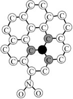
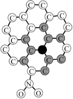
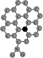
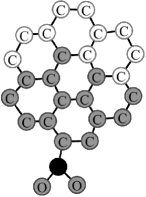
(a)	(b)	(c)	(d)

Figure 4: The receptive field of a neuron in an Ego-CNN effectively enlarges at a deeper layer. (a)-(c) Receptive fields of neurons at the 1st, 2nd, and 5th layer corresponding to the same node. (d) Receptive field of another neuron at the 5th layer that partially covers the graph. The difference in the coverage reflects the position of the corresponding node.

In practice, one should configure the number of layers $L$ (a hyperparameter) according to the diameter of $\mathcal{G}$ to ensure that the critical structures can be detected at the global scale. As large social networks usually manifest the small-world property (Watts & Strogatz, 1998), $L$ is not likely to be a very large number. In addition, one can extend the Ego-CNN model described above in different ways. For example, an Ego-CNN can have different numbers of filters/neurons at different layers. One can also pair up Ego-CNN with an existing node embedding model (Cai et al., 2018) that takes into account node/edge features to compute better $\boldsymbol{H}_{n,:}^{(0)}$ for each node. In fact, Ego-CNN can take any kind of node embeddings as input, as shown in the left of Figure 3.

3.2 Visualizing Critical Structures

Since an Ego-CNN is jointly trained with the task model (to detect task-specific critical structures), the applicable visualization techniques may vary from task to task. Here, we propose a general visualization technique based on the Transposed Deconvolution (Zeiler et al., 2011) that works alongside any task model. It consists of two steps: (1) we add an Attention layer (Itti et al., 1998) between the last Ego-Convolution layer and the first layer of the task model to find the most important neighborhoods at the deepest Ego-Convolution layer. (2) We then use the Transposed Deconvolution to backtrack the nodes in $\mathcal{G}$ that are covered by each of the important neighborhoods identified in Step 1. For more details, please refer to Section 2 of the supplementary materials.

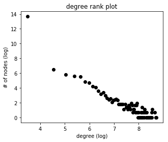
Figure 5: The degree distribution of Reddit dataset follows the power-law distribution.

Table 2: 10-Fold CV test accuracy (%) on bioinfomatic datasets.

Dataset	MUTAG	PTC	PROTEINS	NCI1
Size	188	344	1113	4110
Max #node / #class	28 / 2	64 / 2	620 / 2	125 / 2
WL kernel	82.1	57.0	73.0	82.2
DGK	82.7	57.3	71.7	62.5
Subgraph2vec	87.2	60.1	73.4	80.3
MLG	84.2	63.6	76.1	80.8
Structure2vec	88.3	–	–	83.7
DCNN	67.0	56.6	–	62.6
Patchy-San	92.6	60.0	75.9	78.6
1-head-attention GAT	81.0	57.0	72.5	74.3
Ego-CNN	93.1	63.8	73.8	80.7

We select the neighborhoods with attention scores higher than a predefined threshold in Step 1 as the important ones. Note that the Attention layer (Itti et al., 1998) added in Step 1 does not need to be trained with the Ego-CNN and task models. It can be efficiently trained after the Ego-CNN is trained. To do so, we append the Attention layer and a dense layer with a linear activation function (acting as a linear task model) to the last Ego-Convolution layer of the trained Ego-CNN, then we train the weights of the Attention and dense layers while leaving the weights of the Ego-Convolution layers in the Ego-CNN fixed. The linearity of the task model aligns the attention scores with the importance. This post-visualization technique allows a model user to quickly explore different network configurations for visualization.

3.3 Efficiency and the Scale-Free Prior

Given a graph with $N$ nodes and $D$-dimensional embeddings of nodes, an Ego-CNN with $L$ Ego-Convolution layers base on the top-$K$ neighbors and $D$ filters can embed a graph in $O\left(N(K+1)LD^{2}\right)$ time. For each of the $L$ layers, the $l$-th layer takes $O(NK)$ to lookup and stack up the $K$ neighbors’ embeddings to generate all the $N$ receptive fields of size $(K+1)\times D$, and it takes $O\left(N(K+1)D^{2}\right)$ to have $D$ filters scan through all the receptive fields. The Ego-CNN is highly efficient as compare to existing graph embedding models. Please see Table 1 for more details.

Scale-Free Regularizer. Study (Li et al., 2005) shows that the patterns in a large social network are usually scale-free—the same patterns can be observed at different zoom levels of the network. In practice, one may identify a scale-free network by checking if the node degrees follow a power-law distribution. Figure 5 shows the degree distribution of the Reddit dataset, which is used as one of the datasets in our experiment. The degree distribution follows the power law.

The Ego-CNNs can be readily adapted to detect the scale-free patterns. Recall that the filters at the $l$-th layer detect the patterns of neighborhoods representing the $l$-hop ego networks. By regarding the $1$-hop, $2$-hop, $\cdots$, $L$-hop ego-networks $\boldsymbol{E}^{(n,1)},\boldsymbol{E}^{(n,2)},\cdots,\boldsymbol{E}^{(n,L)}$ centering around the same node $n$ as different “zoom levels” of the graph, we can simply let an Ego-CNN detect the scale-free patterns by tying the weights of filters $\boldsymbol{W}^{(1,d)},\boldsymbol{W}^{(2,d)},\cdots,\boldsymbol{W}^{(L,d)}$ for each $d$. When the input $\mathcal{G}$ is scale-free, this weight-tying technique (a regularization) improves both the performance of the task model and training efficiency.

4 Experiments

In this section, we conduct experiments using real-world datasets to verify (i) Ego-CNNs can lead to comparable task performance as compared to existing graph embedding approaches; (ii) the visualization technique discussed in Section 3.2 can output meaningful critical structures; and (iii) the scale-free regularizer introduced in Section 3.3 can detect the repeating patterns in a scale-free network. All experiments run on a computer with 48-core Intel(R) Xeon(R) E5-2690 CPU, 64 GB RAM, and NVidia Geforce GTX 1070 GPU. We use Tensorflow to implement our methods.

4.1 Graph Classification

We benchmark on both bioinformatic and social-network datasets pre-processed by (Kersting et al., 2016). In the bioinformatic datasets, graphs are provided with node/edge labels and/or attributes, while in the social network datasets, only pure graph structures are given. We consider the task of graph classification. See DGK (Yanardag & Vishwanathan, 2015) for more details about the task and benchmark datasets. We follow DGK to set up the experiments and report the average test accuracy using the 10-fold cross validation (CV). We compare the results Ego-CNN with existing methods mentioned in Section 1 and take the reported accuracy directly from their papers.

Generic Model Settings. To demonstrate the broad applicability of Ego-CNNs, the network architecture of our Ego-CNN implementation remains the same for all datasets. The architecture is composed of 1 node embedding layer (Patchy-San with 128 filters and $K=10$) and 5 Ego-Convolution layers (each with $D=128$ filters and $K=16$) and 2 Dense layers (with 128 neurons for the first Dense layer) as the task model before the output. We apply Dropout (with drop rate $0.5$) and Batch Normalization to the input and Ego-Convolution layers and train the network using the Adam algorithm with learning rate $0.0001$. For selecting the $K$ neighbors, we exploit a heuristic that prefers rare neighbors. We select the top $K$ with the least frequent multiset labels in 1-WL labeling (Weisfeiler & Lehman, 1968). For nodes with less than $K$ neighbors, we simply use zero vectors to represent non-existing neighbors.

The task accuracy are reported in Table 2 and Table 3. Although having fixed architecture, the Ego-CNN is able to give comparable task performance against the stat-of-the-art models (which all use node/edge features) on the bioinformatic datasets. On the social network datasets where the node/edge features are not available, the Ego-CNN is able to outperform previous scalable work. In particular, the Ego-CNN improves the performance of two closely related work, the single-layer Patchy-San and 1-head-attention GAT, on most of the datasets. This justifies that 1) detecting patterns at scales larger than just the adjacent neighbors of each node and 2) allowing full-rank filters/kernels in Eq. (3) are indeed beneficial.

4.2 Visualization of Critical Structures

Chemical Compounds. To justify the usefulness of Ego-CNNs in the cheminformatics problem shown in Figure 1, we generate two compound datasets with critical structures at the local scale (Alkanes vs. Alcohols) and at the global scale (Symmetric vs. Asymmetric Isomers) in the ground truth, respectively. The structures of compounds are generated under different compound size (number of atoms) and vertex-orderings.

Table 3: 10-Fold CV test accuracy (%) on social network datasets.

Dataset	IMDB (B)	IMDB (M)	REDDIT (B)	COLLAB
Size	1000	1000	2000	5000
Max #node / #class	270 / 2	176 / 3	3782 / 2	982 / 3
DGK	67.0	44.6	78.0	73.0
Patchy-San	71.0	45.2	86.3	72.6
1-head-attention GAT	70.0	–	78.8	–
Ego-CNN	72.3	48.1	87.8	74.2

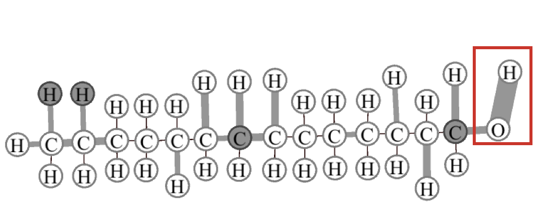
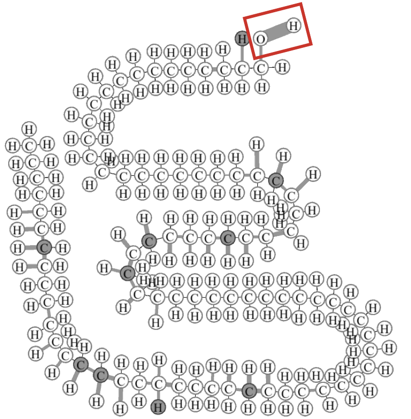
(a) C14 H29 OH	(b) C82 H165 OH
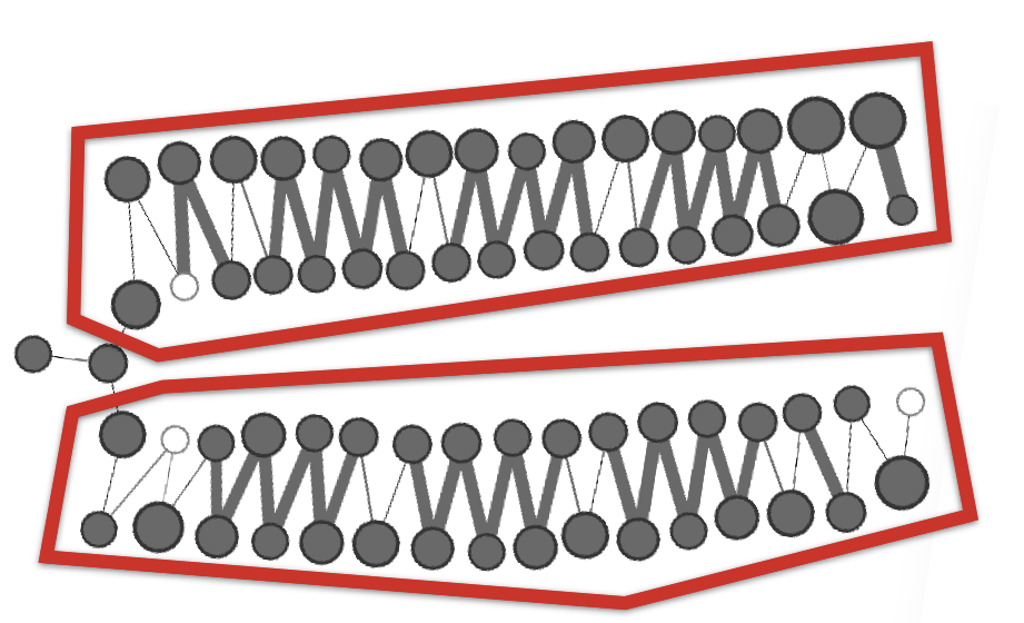
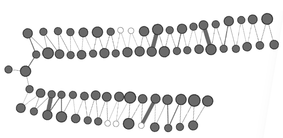
(c) Symmetric Isomer	(d) Asymmetric Isomer

Figure 6: Visualization of critical structures on (a)(b) two Alcohol compounds for the task distinguishing Alcohol from Alkane, and (c) a Symmetric Isomer and (d) an Asymmetric Isomer compounds for the task classifying the types of Isomer. Critical structures are colored in grey and the node/edge size is proportional to its importance. The OH-base on Alcohols is always captured precisely and considered critical. On Symmetric Isomers, the critical patterns are roughly symmetric from the methyl branching node, which shows that the Ego-CNN is able to learn to count from the branching node to see if the structure is symmetric or not.

First, we test if an Ego-CNN considers OH-base as a critical structure in the Alkanes vs. Alcohols dataset. With the post-visualization technique introduced in Section 3.2, we plot the detected critical structures on two Alcohol examples in Figures 6(a)(b). We find that the OH-base on Alcohols is always captured precisely and considered as critical to distinguish Alcohols from Alkanes no matter how large the compounds are.

For Symmetric Isomers like the one shown in Figure 6(c), the Ego-CNN detects the symmetric hydrocarbon chains as critical structures as we expected. An interesting observation is that the importance of the nodes and edge in the detected critical structures are also roughly symmetric to the methyl-base. This symmetry phenomenon can also be observed in the critical structures of the Asymmetric Isomers, as shown in Figure 6(d). We conjecture the Ego-CNN learns to compare if the two long hydrocarbon chains (which are branched from the methyl-base) are symmetric or not by starting comparing the nodes and edges from the methyl-base all along to the end of the hydrocarbon chains, which is similar to how people check if a structure is symmetric.

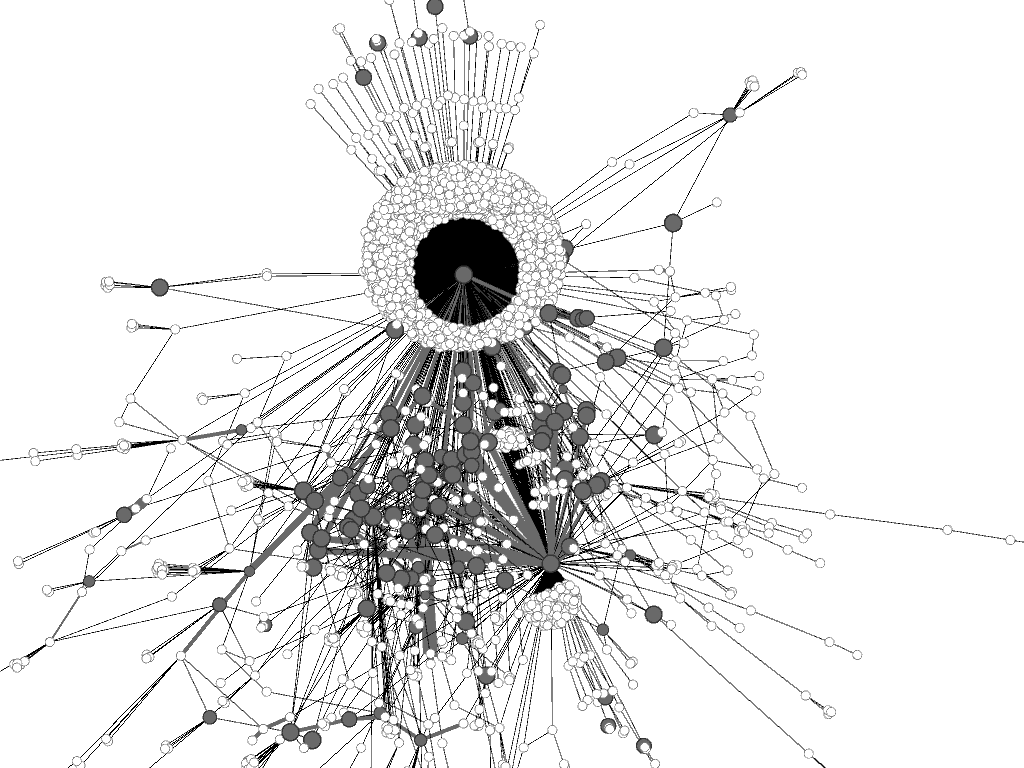
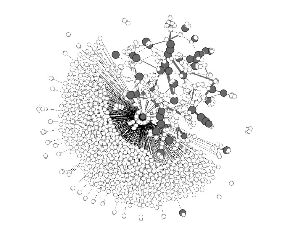
(a) Discussion-based thread.	(b) QA-based thread.

Figure 7: Visualization of critical structures on Reddit dataset. The critical structures are colored in grey and the node/edge size is proportional to its importance. The results show that the variety of different opinions are the key to discriminant discussion-based threads from QA-based threads.

Social Interactions. Without assuming prior knowledge, we visualize the detected critical structures on graphs in the Reddit dataset to see if they can help explain the task predictions. In Reddit dataset, each graph represents a discussion thread. Each node represents a user, and there is an edge if two users have been discussing with each other. The task is to classify the discussion style of the thread into either the discussion-based (e.g. threads under Atheism) or the QA-based (e.g. under AskReddit).

Figure 7 shows the detected critical structures (colored in grey with the node/edge size proportional to its importance). For the discussion-based threads, the Ego-CNN tends to identify users (nodes) that have many connections with other users. On the other hand, many isolated nodes are identified as critical for the QA-based threads. This suggests that the variety of different opinions, which motivate following-up interactions between repliers in a tread, are the key to discriminant discussion-based threads from QA-based threads.

4.3 Scale-Free Regularizer

Next, to verify the effectiveness of the scale-free regularizer proposed in Section 3.3. We compared 1 shallow Ego-CNN (with 1 Ego-Convolution) and 2 deep Ego-CNNs (with 5 Ego-Convolution). All networks are trained on the Reddit dataset with settings described in Section 4.1. Table 4 shows the results.

Table 4: Ego-CNNs on Reddit dataset with the scale-free prior.

Network architecture	Weight-Tying?	10-Fold CV Test Acc (%)	#Params
1 Ego-Conv. layer		84.9	1.3M
5 Ego-Conv. layers		87.8	2.3M
5 Ego-Conv. layers	✓	88.4	1.3M

Without scale-free regularizer, the accuracy improves by 2.9% at the cost of 77% more parameters. Tying the weights of the 5 Ego-Convolution layers, the deep network uses roughly the same amount of parameters as the shallow network but performs better than the network of the same depth without weight-tying. This justifies that the proposed scale-free regularizer can increase both the task performance and training efficiency.

Note, however, that the scale-free regularizer helps only when the graphs are scale-free. When applied to graphs without scale-free properties (e.g., chemical compounds), the scale-free regularizer leads to 2%~10% drop in test accuracy. For more details, please refer to Section 3 of the supplementary materials. This motivates a test like the one shown in Figure 5—one should verify if the target graphs indeed have scale-free properties before applying the scale-free regularizer.

5 Conclusions

We propose Ego-CNNs that employ the Ego-Convolutions to detect invariant patterns among ego networks, and use the ego-centric way to stack up layers to allows to exponentially cover more nodes. The Ego-CNNs work nicely with common visualization techniques to illustrate the detected structures. Investigating the critical structures may help explaining the reasons behind task predictions and/or discovery of new knowledge, which is important to many fields such as the bioinformatics, cheminformatics, and social network analysis. As our future work, we will study how to further improve the time/space efficiency of an Ego-CNN. A neighborhood of a node at a deep layer may overlap with that of another node at the same layer. Therefore, instead of letting a filter scan through all of the neighborhood embeddings at a layer, it might be acceptable to skip some neighborhoods. This can reduce embedding dimensions (space) and speed up computation.

6 Acknowledgments

This work is supported by the MOST Joint Research Center for AI Technology and All Vista Healthcare, Taiwan (MOST 108-2634-F-007-003-). We also thank the anonymous reviewers for their insightful feedbacks.

1 Further Related Work

Here, we give an in-depth review of existing graph embedding models.

Graph Kernels. The Weisfeiler-Lehman kernel (Shervashidze et al., 2011) grows the coverage of each node by collecting information from neighbors, which is conceptually similar to our method, but differs from our model in that WL kernel collects only node labels, while our method collects the complete labeled neighborhood graphs from neighbors. Deep Graph Kernels (Yanardag & Vishwanathan, 2015) and Subgraph2vec (Narayanan et al., 2016), which are inspired by word2vec (Mikolov et al., 2013), embed the graph structure by predicting neighbors’ structures given a node. Multiscale Laplacian Graph Kernels (Kondor & Pan, 2016) compare graphs at multiple scales by recursively comparing graphs based on the comparison of subgraphs, which takes $O(LN^{5})$ where $L$ represents the number of comparing scales and is inefficient. All the above graph kernels have a common drawback in that the embeddings are generated in a unsupervised manner. The critical structure cannot be jointly detected at the generation of embeddings.

Graphical Models. Assuming that the edges of a graph express the conditional dependency between random variables (nodes), Structure2vec (Dai et al., 2016) introduces a novel layer that makes the optimization procedures of approximated inference directly trainable by SGD. It is efficient on large graphs with time complexity linear to number of nodes. However, it’s weak on identifying critical structures because the approximated inference makes too much simplification on the graph structure. For example, the mean-field approximation assumes that variables are independent with each other. As a result, Structure2vec can only identify critical structures of very simple shape.

Convolution-based Methods. Recently, many work are proposed to embed graphs by borrowing the concept of CNN. Figure 8 summarizes the definitions of filters and neighborhoods in these work. The Spatial Graph Convolutional Network (GCN) was proposed by (Bruna et al., 2013). The design of Spatial GCN (Figure 8(a)) is very different from other convolution-based methods (and ours) since its goal is to perform hierarchical clustering of nodes. A neighborhood is defined as a cluster. However, the filter is not aim to scan for local patterns but to learn the connectivity of all clusters. This means each filter is of size $O(N^{2})$ if there are $N$ clusters. Also, a filter requires the global-scale information, i.e. the features of all clusters to train, so it’s very inefficient on large graphs. Hence, in the same paper, (Bruna et al., 2013) proposed another version, the Spectrum GCN, to perform hierarchical clustering in the spectrum domain. The computation of Spectrum GCN is later improved by (Defferrard et al., 2016). However, the major drawback is that the graph spectrum is weak at identifying structures as it is only interpretable for very special graph families (e.g., complete graphs and star-like trees). A recent variant of Spectrum GCN (Kipf & Welling, 2017) uses the filters to detect the propagated feature of each node (equivalent to weighted-sum its neighbors’ features). This variant also cannot detect the critical structures precisely.

(a)	(b)	(c)	(d)	(e)

Figure 8: Filters and neighborhood in (a) Spatial GCN (Bruna et al., 2013). A filter $\boldsymbol{W}$ is a sparse matrix, which is not aimed to detect local patterns, but to learn the connectivity of clusters. (b) DCNN (Atwood & Towsley, 2016) scans through the $M\times N$ diffusion matrix of each node. (c) Patchy-San (Niepert et al., 2016) scans the $K\times K$ adjacency matrix of local neighborhood of each node. (d) Neural Fingerprints (Duvenaud et al., 2015) that scans the $d$-dimensional approximated neighborhood (specially, the summation of neighbors’ embeddings) of each node. (e) Ego-Convolution scans $(K+1)\times D$ egocentric neighborhoods of each node.

Diffusion Convolutional Neural Networks (DCNN) (Atwood & Towsley, 2016) embed the graph by detecting patterns in the diffusion of each node. The neighborhood is defined as the diffusion, which are paths starting from a node to other nodes in $m$ hops. The diffusion can be represented by an $M\times N$ diffusion matrix $\boldsymbol{D}$, where each element $D_{m,n}$ indicates if the current node connects to a node $n$ in $m$ hops. Filters in a DCNN scan through each node’s diffusion matrix. So, DCNN can detect useful diffusion patterns. But it cannot detect critical structures since the diffusion patterns cannot precisely describe the location and the shape of structures. DCNN reported impressive results on the node classification. But it is inefficient on graph classification tasks since their notion of neighborhood is at the global-scale, which takes $O(MN^{2})$ to embed a graph with $N$ nodes. Also, their definition of neighborhood makes the embedding model shallow—there is only one single layer in a DCNN.

Patchy-San (Niepert et al., 2016) uses filters to detects patterns in the adjacency matrix of the $K$ nearest neighbors of each node. The neighborhood of a node $n$ is defined as the $K\times K$ adjacency matrix $\boldsymbol{A}^{(n)}$ of the $K$ nearest neighbors of the node. Filters $\boldsymbol{W}^{(d)}\in\mathbb{R}^{K\times K}$, $d=1,2,\cdots,D$, scan through the adjacency matrix of each node to generate the graph embedding $\boldsymbol{H}\in\mathbb{R}^{N\times D}$, where ${\displaystyle H_{n,d}=\sigma(\bar{\boldsymbol{A}}^{(n)}\varoast\boldsymbol{W}^{(d)}+b_{d}})$ is the output of an activation function $\sigma$, $b_{d}$ is the bias term, and $\varoast$ is the Frobenius inner product defined as $\boldsymbol{X}\varoast\boldsymbol{Y}={\displaystyle\sum_{i,j}X_{i,j}Y_{i,j}}$. Note that a filter scans through $\bar{\boldsymbol{A}}^{(n)}$, the normalized version of $\boldsymbol{A}^{(n)}$ (Niepert et al., 2016), in order to be invariant under different vertex permutations. Patchy-San can detect precise structures (via the filters). However, to detect critical structures at the global level, each $\bar{\boldsymbol{A}}^{(n)}$ needs to have the size of $N\times N$, making the filters $\boldsymbol{W}^{(d)}\in\mathbb{R}^{N\times N}$ hard to learn. There is no discussion on how to generalize the local neighborhood defined by Patchy-San at a deep layer.

The Message-Passing NNs (Duvenaud et al., 2015; Li et al., 2016; Pham et al., 2017; Gilmer et al., 2017; Velickovic et al., 2018; Ying et al., 2018) scan through the approximated neighborhoods of each node and supports multiple layers. At each layer $l$, the neighborhood of a node is defined as a $D$-dimensional vector representing the aggregation (e.g., summation (Duvenaud et al., 2015)) of the $D$-dimensional hidden representation at layer $l-1$ of the $l$-hop neighbors. The summation avoids the vertex-ordering problem of the adjacency matrix in Patchy-San. On the other hand, the Message-Passing NNs loses the ability of detecting precise critical structures.

Note that a Message-Passing NN, called the 1-head-attention graph attention network (1-head GAT) (Velickovic et al., 2018), is a special case of Ego-CNN where the $\boldsymbol{W}^{(l,d)}$ in Eq. (3) in the main paper is replaced by a rank-1 matrix $\boldsymbol{C}^{(l,d)}$. Specifically, it models the $d$-th dimension of the embedding of node $n$ at the $l$-th layer as $H_{n,d}^{(l)}=\sigma\left(\left[\boldsymbol{H}_{Nbr(n,1),:}^{(l-1)},\cdots,\boldsymbol{H}_{Nbr(n,K),:}^{(l-1)}\right]^{\top}\circledast\boldsymbol{C}^{(l,d)}\right)$, where $\boldsymbol{C}^{(l,d)}=\boldsymbol{\alpha}\boldsymbol{W}_{d,:}$ is the outer-product of the edge importance vector $\boldsymbol{\alpha}\in\mathbb{R}^{K}$ and the $d$-th row of their weight matrix $\boldsymbol{W}$. The 1-head GAT was proposed for node classification problems. When it is applied to graph learning tasks, requiring the $\boldsymbol{C}^{(l,d)}$ to be a rank-1 matrix severely limits the model capability and leads to inferior performance.

Model Type	MUTAG	PTC	PROTEINS	NCI1	IMDB (B)	REDDIT (B)
Ego-CNN	93.1 (6s)	63.8 (20s)	73.8 (244s)	80.7 (854s)	72.3	87.8
Patch-San + Std. Convolution Layers	89.4	61.5	70.7	71.0	67.1	81.0
Ego-CNN with Scale-Free Regularizer	84.5 (13s)	59.5 (22s)	73.2 (281s)	77.8 (368s)	71.5	88.4

Figure 9: More experiments.

2 Detailed Visualization Steps

In this section, we detail how the critical structure is visualized using an Ego-CNN. Like standard CNN, each neuron in Ego-CNN represents the matched result for a specific pattern (subgraph) with size upper-bounded by $K^{L}$ nodes. To visualize the detected critical structure, the first step is to to find the most important neighborhoods at the deepest Ego-Convolution layer. The importance score $\gamma^{(n)}$ for each node $n$ can be calculated using the Attention layer described in Section 3.2 of the main paper. Next, we compute the importance-adjusted node embedding $\boldsymbol{\hat{H}}_{n,:}^{(l)}=\gamma^{(n)}\hat{\boldsymbol{H}}_{n,:}^{(l)}\in\mathbb{R}^{D}$ before applying the Transposed Convolution layer-by-layer (from the deepest to the shallowest) to plot the critical subgraphs. At each layer, we (1) follow the Transposed Convolution to re-construct each node’s importance-adjusted neighboring embeddings $\hat{\boldsymbol{E}}^{(n,l)}=\sum_{d}\hat{\boldsymbol{H}}_{n,d}^{(l)}\boldsymbol{W}^{(l,d)}\in\mathbb{R}^{(K+1)\times D}$, and then (2) reconstruct $\boldsymbol{\hat{H}}_{n,:}^{(l-1)}$ by “undoing” $\boldsymbol{E}^{(n,l)}=\left[\boldsymbol{H}_{n,:}^{(l-1)},\boldsymbol{H}_{Nbr(n,1),:}^{(l-1)},\cdots,\boldsymbol{H}_{Nbr(n,K),:}^{(l-1)}\right]^{\top}$ in Eq. (3) in the main paper. We do so by letting $\boldsymbol{\hat{H}}_{n,:}^{(l-1)}=\sum_{i:\text{node }i\text{ is }n\text{\textquoteright s }k\text{-th neightbor, }k\leq K}\hat{\boldsymbol{E}}_{k+1,:}^{(i,l)}$. Repeating the above steps, we end up reconstructing an importance-adjusted adjacency matrix $\hat{\boldsymbol{H}}^{(0)}\in\mathbb{R}^{k\times k}$ that “undoes” Patchy-San. Our Figures 5 and 6 in the main paper plot the graphs using edge widths proportional the values in $\hat{\boldsymbol{H}}^{(0)}$.

3 More Experiments

In this section, we conduct more experiments to further investigate the performance of Ego-CNNs. First, we compare the Ego-CNN with a naive extension of Patch-San using standard CNN layers. The architecture (6 layers) and numbers of parameters of the two models are roughly the same. The results are shown in Figure 9. As we can see, the Ego-CNN with Ego-Convolutions outperforms standard CNN convolutions on graph classification problems.

Next, we compare the Ego-CNNs with and without the scale-free regularizer mentioned in Section 4.3 of the main paper. As we can see in Figure 9, the scale-free regularizer does not boost performance on bioinformatic datasets (MUTAG/PTC/PROTEINS/NCI1) because the graphs have no scale-free property. This motivates a test like the one shown in Figure 5 in the main paper—one should verify if the target graphs indeed have scale-free properties before applying the scale-free regularizer.

4 Relation to Kronecker Graphs

In this section, we brief show how Kronecker graph (Leskovec et al., 2010) is a special case of Ego-CNN with scale-free regularizer. Suppose only 1 pattern $A^{(0)}\in\mathbb{{R}}^{K\times K}$ is captured in the node embedding layer and there is only 1 filter $W\in\mathbb{{R}}^{(K+1)\times 1}$in the weight-tying Ego-Convolution layers. Then, the pattern captured in the $l$-th weight-tying Ego-Convolution filter is $A^{(l)}=f(A^{(l-1)}\bigotimes W)$, where $f$ is a function to convert the list of adjacency matrices of length $K+1$into 1 unified adjacency matrix, where elements that belong to the same physical nodes are merged.

References

- Atwood & Towsley (2016) Atwood, J. and Towsley, D. Diffusion-convolutional neural networks. In Proceedings of NIPS, 2016.
- Bruna et al. (2013) Bruna, J., Zaremba, W., Szlam, A., and LeCun, Y. Spectral networks and locally connected networks on graphs. In Proceedings of ICLR, 2013.
- Cai et al. (2018) Cai, H., Zheng, V. W., and Chang, K. A comprehensive survey of graph embedding: problems, techniques and applications. IEEE Transactions on Knowledge and Data Engineering, 2018.
- Cook (1971) Cook, S. A. The complexity of theorem-proving procedures. In Proceedings of the third annual ACM symposium on Theory of Computing. ACM, 1971.
- Dai et al. (2016) Dai, H., Dai, B., and Song, L. Discriminative embeddings of latent variable models for structured data. In Proceedings of ICML, 2016.
- Defferrard et al. (2016) Defferrard, M., Bresson, X., and Vandergheynst, P. Convolutional neural networks on graphs with fast localized spectral filtering. In Proceedings of NIPS, 2016.
- Duvenaud et al. (2015) Duvenaud, D. K., Maclaurin, D., Iparraguirre, J., Bombarell, R., Hirzel, T., Aspuru-Guzik, A., and Adams, R. P. Convolutional networks on graphs for learning molecular fingerprints. In Proceedings of NIPS, 2015.
- Gilmer et al. (2017) Gilmer, J., Schoenholz, S. S., Riley, P. F., Vinyals, O., and Dahl, G. E. Neural message passing for quantum chemistry. In Proceedings of ICML, 2017.
- Itti et al. (1998) Itti, L., Koch, C., and Niebur, E. A model of saliency-based visual attention for rapid scene analysis. IEEE Transactions on Pattern Analysis and Machine Intelligence, 20(11):1254–1259, 1998.
- Kersting et al. (2016) Kersting, K., Kriege, N. M., Morris, C., Mutzel, P., and Neumann, M. Benchmark data sets for graph kernels, 2016. URL http://graphkernels.cs.tu-dortmund.de.
- Kim et al. (2007) Kim, J., Goh, K.-I., Kahng, B., and Kim, D. A box-covering algorithm for fractal scaling in scale-free networks. Chaos: An Interdisciplinary Journal of Nonlinear Science, 2007.
- Kipf & Welling (2017) Kipf, T. N. and Welling, M. Semi-supervised classification with graph convolutional networks. In Proceedings of ICLR, 2017.
- Kondor & Pan (2016) Kondor, R. and Pan, H. The multiscale laplacian graph kernel. In Proceedings of NIPS, 2016.
- Leskovec et al. (2010) Leskovec, J., Chakrabarti, D., Kleinberg, J., Faloutsos, C., and Ghahramani, Z. Kronecker graphs: An approach to modeling networks. Journal of Machine Learning Research, 11(Feb):985–1042, 2010.
- Li et al. (2005) Li, L., Alderson, D., Doyle, J. C., and Willinger, W. Towards a theory of scale-free graphs: Definition, properties, and implications. Internet Mathematics, pp. 431–523, 2005.
- Li et al. (2016) Li, Y., Tarlow, D., Brockschmidt, M., and Zemel, R. Gated graph sequence neural networks. In Proceedings of ICLR, 2016.
- Mikolov et al. (2013) Mikolov, T., Chen, K., Corrado, G., and Dean, J. Efficient estimation of word representations in vector space. 2013.
- Narayanan et al. (2016) Narayanan, A., Chandramohan, M., Chen, L., Liu, Y., and Saminathan, S. subgraph2vec: Learning distributed representations of rooted sub-graphs from large graphs. In Workshop on Mining and Learning with Graphs, 2016.
- Niepert et al. (2016) Niepert, M., Ahmed, M., and Kutzkov, K. Learning convolutional neural networks for graphs. In Proceedings of ICML, 2016.
- Pham et al. (2017) Pham, T., Tran, T., Phung, D. Q., and Venkatesh, S. Column networks for collective classification. In Proceedings of AAAI, 2017.
- Shervashidze et al. (2011) Shervashidze, N., Schweitzer, P., Leeuwen, E. J. v., Mehlhorn, K., and Borgwardt, K. M. Weisfeiler-lehman graph kernels. JMLR, 12(Sep):2539–2561, 2011.
- Velickovic et al. (2018) Velickovic, P., Cucurull, G., Casanova, A., Romero, A., Lio, P., and Bengio, Y. Graph attention networks. In Proceedings of ICLR, 2018.
- Watts & Strogatz (1998) Watts, D. J. and Strogatz, S. H. Collective dynamics of small-worldnetworks. Nature, 393(6684):440, 1998.
- Weisfeiler & Lehman (1968) Weisfeiler, B. and Lehman, A. A reduction of a graph to a canonical form and an algebra arising during this reduction. Nauchno-Technicheskaya Informatsia, 2(9):12–16, 1968.
- Yanardag & Vishwanathan (2015) Yanardag, P. and Vishwanathan, S. Deep graph kernels. In Proceedings of SIGKDD. ACM, 2015.
- Ying et al. (2018) Ying, Z., You, J., Morris, C., Ren, X., Hamilton, W., and Leskovec, J. Hierarchical graph representation learning with differentiable pooling. In Proceedings of NIPS, pp. 4805–4815, 2018.
- Zeiler et al. (2011) Zeiler, M. D., Taylor, G. W., and Fergus, R. Adaptive deconvolutional networks for mid and high level feature learning. In Proceedings of ICCV. IEEE, 2011.