Changing Fock matrix elements of two-mode squeezed vacuum state by employing three conditional operations in one-sided lossy channel

Abstract

This paper focuses on changing Fock matrix elements of two-mode squeezed vacuum state (TMSVS) by employing three conditional operations in one-sided lossy channel. These three conditional operations include one-photon replacement (OPR), one-photon substraction (OPS) and one-photon addition (OPA). Indeed, three conditional quantum states have been generated from the original TMSVS. Using the characteristic function (CF) representation of quantum density operator, we derive the analytical expressions of their Fock matrix elements, which depend on the interaction parameters, including the squeezing parameter of the input TMSVS, the loss factor and the transmissivity of the variable beam splitter. For convenience of discussion, we only give the Fock matrices in the subspace span $\left\{\left|00\right\rangle,\left|01\right\rangle,\left|10\right\rangle,\left|02\right\rangle,\left|11\right\rangle,\left|20\right\rangle\right\}$ for these two-mode states. Obviously, the TMSVS only has the populations in $\left|00\right\rangle$ and $\left|11\right\rangle$ in such subspace. By comparing the generated states with the TMSVS, we find that: (1) The generated state after OPR will remain the populations in $\left|00\right\rangle$ and $\left|11\right\rangle$, and add the populations in $\left|10\right\rangle$ and $\left|20\right\rangle$; (2) The generated state after OPS will lost the populations in $\left|00\right\rangle$ and $\left|11\right\rangle$, but add the populations in $\left|10\right\rangle$ and $\left|20\right\rangle$; (3) The generated state after OPA will remain the population only in $\left|11\right\rangle$ and add the population in $\left|01\right\rangle$.

Keywords: two-mode squeezed vacuum state, Fock matrix elements; twin-Fock state, conditional measurement, beam splitter, characteristic function

I Introduction

Quantum state tomography, as a standard approach to characterize unknown quantum state, is often to construct a density matrix from which some other information can be inferred. People can retrieve desired information about a quantum state by performing multiple tomographic measurements (also the so-called projective measurements in different bases) a1 . The most common measurement is the homodyne measurement. Through homodyne measurement, one can obtain a large amount of data, which can be converted into the state’s density matrix and/or Wigner function by resorting to mathematical methods, such as the inverse Randon transformation, the pattern-function method and the likelihood maximization algorithm a2 . In other words, the unknown quantum state can be reconstructed in the representation of a density matrix, either in the quadrature basis or in the photon-number (Fock) basis. Recently, complete information about excited coherent states has been analyzed by the optical tomography by Almarashia and co-worker a3 .

Theoretically, in order to find the information of quantum state, one choose projection operator in photon-number (Fock) basis to obtain its Fock matrix elements. Indeed, every quantum state can be expanded in the number state space and has its unique Fock matrix elements. For a one-mode quantum state, the density operator $\rho$ can be written as $\rho=\sum_{n,m=0}^{\infty}p_{mn}\left|m\right\rangle\left\langle n\right|$ with $p_{mn}=\left\langle m\right|\rho\left|n\right\rangle$, in which the Fock matrix elements $p_{mn}$ is corresponding to component $\left|n\right\rangle\left\langle m\right|$ in the space of density operator $\rho$. It should be emphasized that the elements $p_{mn}$ represent populations (diagonal term $n=m$, real number) or coherences (off-diagonal $n\neq m$, often complex number). For example, the familiar thermal state, as a mixed state, has only the components $\left|n\right\rangle\left\langle n\right|$ ($n=0,1,2,\cdots$) with population element $p_{nn}$. The coherent state, as a typical pure state, has the components $\left|n\right\rangle\left\langle m\right|$ ($n,m=0,1,2,\cdots$) with elements $p_{nm}$ (population or coherence). The single-mode squeezed vacuum state, also a pure state, has only the components $\left|2n\right\rangle\left\langle 2m\right|$ ($n,m=0,1,2,\cdots$) with elements $p_{2n,2m}$ 1 ; 2 , which often was used as the typical optical field interacting with atomical system 2a ; 2b .

Similarly, for a two-mode case, the density operator $\rho_{ab}$ can be written in the two-mode photon-number basis

$$\rho_{ab}=\sum_{n_{1},m_{1},n_{2},m_{2}=0}^{\infty}p_{n_{1}m_{1},n_{2}m_{2}}\left|n_{1}\right\rangle_{a}\left|m_{1}\right\rangle_{b}\left\langle n_{2}\right|_{a}\left\langle m_{2}\right|_{b},$$ (1)

with $p_{n_{1}m_{1},n_{2}m_{2}}=\left\langle n_{1}\right|_{a}\left\langle m_{1}\right|_{b}\rho_{ab}\left|n_{2}\right\rangle_{a}\left|m_{2}\right\rangle_{b}$, which shows Fock matrix element $p_{n_{1}m_{1},n_{2}m_{2}}$ corresponding to component $\left|n_{1}\right\rangle_{a}\left|m_{1}\right\rangle_{b}\left\langle n_{2}\right|_{a}\left\langle m_{2}\right|_{b}$ in the space of two-mode density operator $\rho_{ab}$ 3 ; 4 . It should be noted that $\left|n\right\rangle_{a}\left|m\right\rangle_{b}$ is often written as $\left|nm\right\rangle$ in this paper. Because the space of the two-mode density operator has infinite two-mode number bases span $\left\{\left|nm\right\rangle\right\}$ ($n,m=0,1,\cdots,\infty$), we only study the Fock matrix elements in the subspace span $\left\{\left|00\right\rangle,\left|01\right\rangle,\left|10\right\rangle,\left|02\right\rangle,\left|11\right\rangle,\left|20\right\rangle\right\}$ for convenience of discussion, whose corresponding Fock matrix can also be expressed in Table I.  As we all know, the two-mode squeezed vacuum state (TMSVS) is the primary entangled resource in continuous-variable system, which can be used to implement many quantum protocols, including continuous version of teleportation and quantum key distribution. In addition, as a maximum entangled state, the TMSVS has also been chosen as the typical optical field interacting with atomical system 4a . Indeed, as a typical two-mode quantum state, the TMSVS has only the twin-Fock components with the form $\left|nn\right\rangle\left\langle mm\right|$ ($n,m=0,1,2,\cdots$). Needless to say, it is impossible to have non-twin-Fock components for the TMSVS. Therefore, it is urgent for us to think that whether we have some ways to change the Fock matrix elements for the TMSVS by using quantum operations. This is the key aim of our paper.

Table 1: Fock matrix elements of two-mode density operator $\rho$ in subspace span $\left\{\left|00\right\rangle,\left|01\right\rangle,\left|10\right\rangle,\left|02\right\rangle,\left|11\right\rangle,\left|20\right\rangle,\cdots\right\}$

$\rho$	$\left|00\right\rangle$	$\left|01\right\rangle$	$\left|10\right\rangle$	$\left|02\right\rangle$	$\left|11\right\rangle$	$\left|20\right\rangle$	$\cdots$
$\left\langle 00\right|$	$p_{00,00}$	$p_{00,01}$	$p_{00,10}$	$p_{00,02}$	$p_{00,11}$	$p_{00,20}$	$\cdots$
$\left\langle 01\right|$	$p_{01,00}$	$p_{01,01}$	$p_{01,10}$	$p_{01,02}$	$p_{01,11}$	$p_{01,20}$	$\cdots$
$\left\langle 10\right|$	$p_{10,00}$	$p_{10,01}$	$p_{10,10}$	$p_{10,02}$	$p_{10,11}$	$p_{10,20}$	$\cdots$
$\left\langle 02\right|$	$p_{02,00}$	$p_{02,01}$	$p_{02,10}$	$p_{02,02}$	$p_{02,11}$	$p_{02,20}$	$\cdots$
$\left\langle 11\right|$	$p_{11,00}$	$p_{11,01}$	$p_{11,10}$	$p_{11,02}$	$p_{11,11}$	$p_{11,20}$	$\cdots$
$\left\langle 20\right|$	$p_{20,00}$	$p_{20,01}$	$p_{20,10}$	$p_{20,02}$	$p_{20,11}$	$p_{20,20}$	$\cdots$
$\vdots$	$\vdots$	$\vdots$	$\vdots$	$\vdots$	$\vdots$	$\vdots$	$\ddots$

In recent years, some conditional operations, such as photon replacement, photon subtraction and photon addition, have attracted extensive attention of researchers. In fact, these schemes are related to conditional measurements, which are fruitful methods for quantum-state manipulation and engineering 5 . Many nonclassical states have been generated by conditional measurements theoretically or experimentally. In general, two quantum states in the two output ports of the lossless beam splitter (BS) are quantum-mechanically correlated with each other. If appropriate measurement is employed in one of the output ports, then conditional quantum state is generated in the other output port 6 ; 7 . In some conditional measurement schemes, new output state $\rho_{out}$ is generated from the input state $\rho_{in}$ in the main channel and the difference happen in the ancillary channel. For example, photon-replacement scheme has the feature that $m$-photon Fock state is input and the same $m$-photon Fock state is measured in ancillary channel. This strategy is also called as “quantum-optical catalysis” 8 ; 9 ; 10 . The photon-subtraction scheme has the feature that $m$-photon Fock state is input and the bigger $n$-photon Fock state is measured in ancillary channel 11 ; 12 ; 13 . The photon-addition scheme has the feature that $m$-photon Fock state is input and the smaller $n$-photon Fock state is measured in ancillary channel 14 ; 15 . These non-Gaussian conditional operations have proven advantageous in many scenarios such as entanglement enhancement 16 ; 17 and teleportation improvement 18 ; 19 . On the other hand, the loss accompanied by conditional operations is unavoidable, which must be considered in realistic situation. Of course, losses may in principle be overcome by some quantum techniques 20 ; 21 ; 22 ; 23 .

Combining with the above ideas and approaches, we aim to change the Fock matrix elements of the TMSVS by employing conditional operations and considering the loss. The Fock matrix elements before and after operations are compared. Analytical and numerical results will be given in details. The paper is organized as follows: In Sec.2, we make a brief review of the TMSVS and introduce its Fock matrix elements. Here we raise the question of how their elements will be changed. In Sec.3, we induce three quantum states from the TMSVS, whose density operators are given. Sec.4 gives the analytical expressions of Fock matrix elements for three generated states. Numerical calculations about elements are made by choosing given interaction parameters in Sec.5. Our conclusions are summarized in the last section.

II Two-mode squeezed vacuum state and its Fock matrix elements

In this section, we make a brief review of the TMSVS and introduce its Fock matrix elements. To begin with, we introduce the two-mode squeezing operator 24

$$S\left(r\right)=\exp[r(a^{{\dagger}}b^{{\dagger}}-ab)],$$ (2)

where $a$ and $b$ are the annihilation operators for the two modes and $r$ is the real squeezing parameter. By operating $S\left(r\right)$ on the two-mode vacuum $\left|00\right\rangle$, we can obtain the TMSVS

$$S\left(r\right)\left|00\right\rangle=\sqrt{1-\lambda^{2}}\exp\left(\lambda a^{{\dagger}}b^{{\dagger}}\right)\left|00\right\rangle$$ (3)

with $\lambda=\tanh r$. Obviously, the TMSVS can be written in number basis as follows

$$S\left(r\right)\left|00\right\rangle=\sum_{n=0}^{\infty}c_{n}\left|nn\right\rangle=c_{0}\left|00\right\rangle+c_{1}\left|11\right\rangle+\cdots$$ (4)

with $c_{n}=\lambda^{n}\sqrt{1-\lambda^{2}}$. The obvious fact is that the TMSVS is only the superposition of the twin Fock state, that is, $\left|00\right\rangle$, $\left|11\right\rangle$, $\cdots$ . It’s impossible for the TMSVS to contain non-twin-Fock state $\left|nm\right\rangle$ with $n\neq m$, such as $\left|01\right\rangle$, $\left|10\right\rangle$, $\left|02\right\rangle$, $\left|12\right\rangle$, $\cdots$ .

Correspondingly, the density operator of the TMSVS can be expressed as

$$\rho_{TMSVS}=S\left(r\right)\left|00\right\rangle\left\langle 00\right|S^{{\dagger}}\left(r\right).$$ (5)

Using Eq.(4), it can be also expanded as

$$\rho_{TMSVS} = c_{0}c_{0}\left|00\right\rangle\left\langle 00\right|+c_{0}c_{1}\left|00\right\rangle\left\langle 11\right|+\cdots$$ (6)

$$+c_{1}c_{0}\left|11\right\rangle\left\langle 00\right|+c_{1}c_{1}\left|11\right\rangle\left\langle 11\right|+\cdots$$

$$+\cdots,$$

where the density operator only contains the twin-Fock components. Obviously, in our considered subspace, we find that the TMSVS has only component $\left|00\right\rangle\left\langle 00\right|$ with population probability $c_{0}c_{0}=1-\lambda^{2}$ and component $\left|11\right\rangle\left\langle 11\right|$ with population probability $c_{1}c_{1}=\lambda^{2}\left(1-\lambda^{2}\right)$. Of course, there are other two coherence terms (i.e., corresponding to components $\left|00\right\rangle\left\langle 11\right|$ and $\left|11\right\rangle\left\langle 00\right|$) as non-zero elements in matrix, which is the coherence between $\left|00\right\rangle$ and $\left|11\right\rangle$. Table II gives the Fock matrix elements of the TMSVS.

Now another question arises: what can we do to make the TMSVS to contain elements corresponding to non-twin-Fock components, such as $\left|00\right\rangle\left\langle 01\right|$ and $\left|01\right\rangle\left\langle 10\right|$? This will be the focus of our following work.

Table 2: Fock matrix elements of the TMSVS in subspace span $\left\{\left|00\right\rangle,\left|01\right\rangle,\left|10\right\rangle,\left|02\right\rangle,\left|11\right\rangle,\left|20\right\rangle,\cdots\right\}$

$\rho_{TMSVS}$	$\left|00\right\rangle$	$\left|01\right\rangle$	$\left|10\right\rangle$	$\left|02\right\rangle$	$\left|11\right\rangle$	$\left|20\right\rangle$	$\cdots$
$\left\langle 00\right|$	$1-\lambda^{2}$	$0$	$0$	$0$	$\lambda\left(1-\lambda^{2}\right)$	$0$	$\cdots$
$\left\langle 01\right|$	$0$	$0$	$0$	$0$	$0$	$0$	$\cdots$
$\left\langle 10\right|$	$0$	$0$	$0$	$0$	$0$	$0$	$\cdots$
$\left\langle 02\right|$	$0$	$0$	$0$	$0$	$0$	$0$	$\cdots$
$\left\langle 11\right|$	$\lambda\left(1-\lambda^{2}\right)$	$0$	$0$	$0$	$\lambda^{2}\left(1-\lambda^{2}\right)$	$0$	$\cdots$
$\left\langle 20\right|$	$0$	$0$	$0$	$0$	$0$	$0$	$\cdots$
$\vdots$	$\vdots$	$\vdots$	$\vdots$	$\vdots$	$\vdots$	$\vdots$	$\ddots$

III Three quantum states induced from the TMSVS

As shown in Fig.1, we construct three conceptual schemes to generate three new quantum states from the TMSVS. Using the TMSVS as the initial optical field and operating three kinds of non-Gaussian conditional operations in one mode (channel) which has the loss, we study and compare the Fock matrix elements of the final optical fields. Using the characteristic function (CF) representation, we obtain the normal forms (denoted by $\colon\colon$) for every density operator. Of course, the success probabilities are also obtained.

The propagation of optical field in every scheme includes two input-output processes and three stages. The two processes include loss and non-Gaussian operation, respectively. For the sake of convenience, we describe the optical field in every stages with their corresponding density operators as follows

$$\rho_{ab}^{\left(I\right)}\Rightarrow\rho_{ab}^{\left(II\right)}\Rightarrow\rho_{ab}^{\left(III\right)}.$$ (7)

Next we shall give the exact expressions of the density operator in every stages.

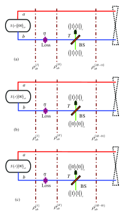
Figure 1: (Colour online) Three conceptual quantum schemes to obtain quantum states from the TMSV. The operations include (a) OPR, (b) OPS and (c) OPA, where the loss is also considered. Here $\eta$ is the loss factor and $T$ is transmissivity of the BS.

Stage 1: The corresponding density operator in stage 1 is $\rho_{ab}^{\left(I\right)}=\rho_{TMSVS}$, where the initial optical field under consideration is the TMSVS $S\left(r\right)\left|00\right\rangle$. By using the Weyl expansion of the density operator, $\rho_{ab}^{\left(I\right)}$ can also be expressed furtherly in the CF representation as follows

$$\rho_{ab}^{\left(I\right)}=\int\frac{d^{2}\alpha d^{2}\beta}{\pi^{2}}\chi_{ab}^{\left(I\right)}\left(\alpha,\beta\right)D_{a}\left(-\alpha\right)D_{b}\left(-\beta\right),$$ (8)

where

$$\chi_{ab}^{\left(I\right)}\left(\alpha,\beta\right) = \mathrm{Tr}(\rho_{ab}^{\left(I\right)}D_{a}\left(\alpha\right)D_{b}\left(\beta\right))$$ (9)

$$= e^{-\frac{(1+\lambda^{2})(\left|\alpha\right|^{2}+\left|\beta\right|^{2})}{2(1-\lambda^{2})}+\frac{\lambda(\allowbreak\alpha^{\ast}\beta^{\ast}+\alpha\beta)}{1-\lambda^{2}}}$$

is just the CF of the TMSVS and $D_{a}\left(\alpha\right)=\exp\left(\alpha a^{{\dagger}}-\alpha^{\ast}a\right)$ and $D_{b}\left(\beta\right)=\exp\left(\beta b^{{\dagger}}-\beta^{\ast}b\right)$ are the displacement operators, respectively.

Stage 2: In the second stage, we consider the loss only in channel (mode) $b$, where the conditional operation will be employed. Thus, the density operator of the optical field can be expressed as

$$\rho_{ab}^{\left(II\right)} = \int\frac{d^{2}\alpha d^{2}\beta}{\pi^{2}}e^{-\frac{1}{2}\eta\left|\beta\right|^{2}}\chi_{ab}^{\left(I\right)}(\alpha,\sqrt{1-\eta}\beta)$$ (10)

$$\times D_{a}\left(-\alpha\right)D_{b}\left(-\beta\right),$$

where $\eta\in\left[0,1\right]$ is the loss factor. Here one can use the formula derived in Ref.25 or see Appendix A.

Stage 3: There are the differences for the three sub-figures of Fig.1 in this stage. Three conditional operations (that is, one-photon replacement (OPR), one-photon subtraction (OPS) and one-photon addition (OPA)) are used in three schemes, respectively.

Case OPR: The OPR can be embodied in the $c$ mode, where one-photon Fock state $\left|1\right\rangle$ is input and one-photon Fock state $\left|1\right\rangle$ is measured 26 . After employing the OPR, we obtain the first generating state

$$\rho_{ab}^{\left(III-11\right)}=\frac{{}_{c}\left\langle 1\right|\{B[\rho_{ab}^{\left(II\right)}\otimes\left(\left|1\right\rangle\left\langle 1\right|\right)_{c}]B^{{\dagger}}\}\left|1\right\rangle_{c}}{p_{d}^{\left(11\right)}},$$ (11)

where $p_{d}^{\left(11\right)}$ is the success probability and $B=\exp\left[\theta\left(b^{{\dagger}}c-bc^{{\dagger}}\right)\right]$ is the BS operator satisfying the following transformation

$$BbB^{{\dagger}} = \sqrt{T}b+\sqrt{1-T}c,$$

$$BcB^{{\dagger}} = -\sqrt{1-T}b+\sqrt{T}c,$$ (12)

with transmissivity $T=\cos^{2}\theta$. After detailed calculation, we obtain the density operator in the normal ordering form

$$\rho_{ab}^{\left(III-11\right)} =\frac{1-\lambda^{2}}{p_{d}^{\left(11\right)}}\frac{d^{4}}{dh_{2}dh_{1}ds_{2}ds_{1}}$$

$$\colon e^{-(\allowbreak 1-\lambda^{2}\eta)a^{{\dagger}}a+\lambda\sqrt{1-\eta}\allowbreak\sqrt{1-T}\left(h_{2}a^{{\dagger}}+h_{1}a\right)}$$

$$\times e^{-b^{{\dagger}}b-\sqrt{1-T}\left(s_{1}b^{{\dagger}}+s_{2}b\right)+\lambda\sqrt{1-\eta}\sqrt{T}\left(a^{{\dagger}}b^{{\dagger}}+ab\right)}$$

$$\times e^{\sqrt{T}h_{2}s_{1}+\sqrt{T}h_{1}s_{2}}\colon|_{s_{1}=s_{2}=h_{1}=h_{2}=0},$$ (13)

where

$$p_{d}^{\left(11\right)}=\Omega^{3}\left(1-\lambda^{2}\right)\left(T+\kappa_{1}\lambda^{2}+\kappa_{2}\lambda^{4}\right)$$ (14)

is the success probability (also the normalization factor), whose derivative form can be found in the appendix B, with

$$\Omega^{-1} = 1-\lambda^{2}\eta-T\lambda^{2}\left(1-\allowbreak\eta\right),$$

$$\kappa_{1} = \left(1+T^{2}\right)\left(1-\eta\right)+2T\left(\eta-2\right),$$

$$\kappa_{2} = T-\eta\left(1-\eta\right)\left(1-T\right)^{2}.$$ (15)

Obviously, if $\eta\rightarrow 0$ and $T\rightarrow 1$, then $\rho_{ab}^{\left(III-11\right)}\rightarrow\rho_{ab}^{\left(I\right)}$. That is, the first generated state can be reduced to the TMSVS in this limit case.

Case OPS: The OPS can be embodied in the $c$ mode, where vacuum state $\left|0\right\rangle$ is input and one-photon Fock state $\left|1\right\rangle$ is measured. After employing the OPS, we obtain the second generating state

$$\rho_{ab}^{\left(III-01\right)}=\frac{{}_{c}\left\langle 1\right|\{B[\rho_{ab}^{\left(II\right)}\otimes\left(\left|0\right\rangle\left\langle 0\right|\right)_{c}]B^{{\dagger}}\}\left|1\right\rangle_{c}}{p_{d}^{\left(01\right)}},$$ (16)

where $p_{d}^{\left(01\right)}$ is the success probability. The density operator in the normal ordering form can be expressed as

$$\rho_{ab}^{\left(III-01\right)} =\frac{\allowbreak 1-\lambda^{2}}{p_{d}^{\left(01\right)}}\frac{d^{2}}{dh_{2}dh_{1}}$$

$$\colon e^{-(\allowbreak 1-\lambda^{2}\eta)a^{{\dagger}}a+\lambda\sqrt{1-\eta}\allowbreak\sqrt{1-T}\left(h_{2}a^{{\dagger}}+h_{1}a\right)}$$

$$\times e^{-b^{{\dagger}}b+\lambda\sqrt{1-\eta}\sqrt{T}\left(a^{{\dagger}}b^{{\dagger}}+ab\right)}\colon|_{h_{1}=h_{2}=0}$$ (17)

with the success probability

$$p_{d}^{\left(01\right)}=\Omega^{2}\lambda^{2}\left(1-\lambda^{2}\right)\left(1-\eta\right)\left(1-T\right).$$ (18)

Case OPA: The OPA can be embodied in the $c$ mode, where one-photon Fock state $\left|1\right\rangle$ is input and vacuum state $\left|0\right\rangle$ is measured. After employing the OPA, we obtain the third generating state

$$\rho_{ab}^{\left(III-10\right)}=\frac{{}_{c}\left\langle 0\right|\{B[\rho_{ab}^{\left(II\right)}\otimes\left(\left|1\right\rangle\left\langle 1\right|\right)_{c}]B^{{\dagger}}\}\left|0\right\rangle_{c}}{p_{d}^{\left(10\right)}},$$ (19)

where $p_{d}^{\left(10\right)}$ is the success probability. The density operator in the normal ordering form can be expressed as

$$\rho_{ab}^{\left(III-10\right)} = \frac{\allowbreak 1-\lambda^{2}}{p_{d}^{\left(10\right)}}\frac{d^{2}}{ds_{2}ds_{1}}$$ (20)

$$\colon e^{-(\allowbreak 1-\lambda^{2}\eta)a^{{\dagger}}a+\lambda\sqrt{1-\eta}\sqrt{T}\left(a^{{\dagger}}b^{{\dagger}}+ab\right)}$$

$$\times e^{-b^{{\dagger}}b-\sqrt{1-T}\left(s_{1}b^{{\dagger}}+s_{2}b\right)}\colon|_{s_{1}=s_{2}=0}$$

with the success probability

$$p_{d}^{\left(10\right)}=\Omega^{2}\left(1-\lambda^{2}\right)\left(1-\lambda^{2}\eta\right)\left(1-T\right).$$ (21)

Obviously, these new generating states can be adjusted by the interaction parameters, including the squeezing parameter $r$ of the input TMSV, the loss factor $\eta$, and the transmissivity $T$ of BS.

IV Fock matrix elements for three generated states

Next, we study the Fock matrix elements for three generated states, which will be compared with that of the original TMSVS. Firstly, we give their analytical expressions for the Fock matrix elements and then give the Fock matrix. As example, we plot the Fock matrices for these states and the population elements by choosing given interaction parameters.

IV.1 Analytical expressions

After detailed derivation, we obtain the following analytical expressions of the Fock matrix elements for every quantum states.

(1) For $\rho_{ab}^{\left(III-11\right)}$, we have

$$p_{n_{1}m_{1},n_{2}m_{2}}^{\left(11\right)} =\frac{\allowbreak 1-\lambda^{2}}{p_{d}^{\left(11\right)}\sqrt{n_{1}!n_{2}!m_{1}!m_{2}!}}$$

$$\frac{d^{n_{1}+n_{2}+m_{1}+m_{2}}}{dg_{2}^{m_{2}}dg_{1}^{m_{1}}df_{2}^{n_{2}}df_{1}^{n_{1}}}\frac{d^{4}}{ds_{1}ds_{2}dh_{1}dh_{2}}$$

$$e^{\lambda\sqrt{1-\eta}\allowbreak[\sqrt{1-T}\left(f_{1}h_{2}+h_{1}f_{2}\right)+\sqrt{T}\left(f_{1}g_{1}+f_{2}g_{2}\right)]}$$

$$\times e^{\sqrt{T}\left(h_{2}s_{1}+h_{1}s_{2}\right)-\sqrt{1-T}\left(g_{1}s_{1}+g_{2}s_{2}\right)}$$

$$\times e^{{}^{\lambda^{2}\eta f_{1}f_{2}}\allowbreak}|_{f_{1}=f_{2}=g_{1}=g_{2}=h_{1}=h_{2}=s_{1}=s_{2}=0}.$$ (22)

(2) For $\rho_{ab}^{\left(III-01\right)}$, we have

$$p_{n_{1}m_{1},n_{2}m_{2}}^{\left(01\right)} =\frac{\allowbreak 1-\lambda^{2}}{p_{d}^{\left(01\right)}\sqrt{n_{1}!n_{2}!m_{1}!m_{2}!}}$$

$$\frac{d^{n_{1}+n_{2}+m_{1}+m_{2}}}{dg_{2}^{m_{2}}dg_{1}^{m_{1}}df_{2}^{n_{2}}df_{1}^{n_{1}}}\frac{d^{2}}{dh_{1}dh_{2}}$$

$$e^{\lambda\sqrt{1-\eta}\allowbreak[\sqrt{1-T}\left(f_{1}h_{2}+h_{1}f_{2}\right)+\sqrt{T}\left(f_{1}g_{1}+f_{2}g_{2}\right)]}$$

$$\times e^{\lambda^{2}\eta f_{1}f_{2}\allowbreak}|_{f_{1}=f_{2}=g_{1}=g_{2}=h_{1}=h_{2}=0}.$$ (23)

(3) For $\rho_{ab}^{\left(III-10\right)}$, we have

$$p_{n_{1}m_{1},n_{2}m_{2}}^{\left(10\right)} =\frac{\allowbreak 1-\lambda^{2}}{p_{d}^{\left(10\right)}\sqrt{n_{1}!n_{2}!m_{1}!m_{2}!}}$$

$$\frac{d^{n_{1}+n_{2}+m_{1}+m_{2}}}{dg_{2}^{m_{2}}dg_{1}^{m_{1}}df_{2}^{n_{2}}df_{1}^{n_{1}}}\frac{d^{2}}{ds_{1}ds_{2}}$$

$$e^{\lambda\sqrt{1-\eta}\allowbreak\sqrt{T}\left(f_{1}g_{1}+f_{2}g_{2}\right)-\sqrt{1-T}\left(g_{1}s_{1}+g_{2}s_{2}\right)}$$

$$\times e^{\lambda^{2}\eta f_{1}f_{2}}|_{f_{1}=f_{2}=g_{1}=g_{2}=s_{1}=s_{2}=0}.$$ (24)

It should be noted that these expressions retain the derivative form because of the complexity of components. With these expressions, we can calculate the matrix elements in each case by mathematical software.

IV.2 Matrix forms and Numerical results

In the considered subspace, we give the Fock matrix elements of state $\rho_{ab}^{\left(III-11\right)}$ in Table III, where the non-zero elements elements are

$$p_{00,00}^{\left(11\right)} = \frac{T\left(1-\lambda^{2}\right)}{p_{d}^{\left(11\right)}},p_{10,10}^{\left(11\right)}=\frac{\eta T\lambda^{2}\left(1-\lambda^{2}\right)}{p_{d}^{\left(11\right)}},$$

$$p_{00,11}^{\left(11\right)} = p_{11,00}^{\left(11\right)}=\frac{\sqrt{T\left(1-\eta\right)}\lambda\left(2T-1\right)\left(1-\lambda^{2}\right)}{p_{d}^{\left(11\right)}},$$

$$p_{11,11}^{\left(11\right)} = \frac{\left(1-\eta\right)\left(2T-1\right)^{2}\lambda^{2}\left(1-\lambda^{2}\right)}{p_{d}^{\left(11\right)}},$$

$$p_{20,20}^{\left(11\right)} = \frac{T\eta^{2}\lambda^{4}\left(1-\lambda^{2}\right)}{p_{d}^{\left(11\right)}}.$$ (25)

Table 3: Fock matrix elements of state $\rho_{ab}^{\left(III-11\right)}$ in subspace span $\left\{\left|00\right\rangle,\left|01\right\rangle,\left|10\right\rangle,\left|02\right\rangle,\left|11\right\rangle,\left|20\right\rangle,\cdots\right\}$

$\rho_{ab}^{\left(III-11\right)}$	$\left|00\right\rangle$	$\left|01\right\rangle$	$\left|10\right\rangle$	$\left|02\right\rangle$	$\left|11\right\rangle$	$\left|20\right\rangle$	$\cdots$
$\left\langle 00\right|$	$p_{00,00}^{\left(11\right)}$	$0$	$0$	$0$	$p_{00,11}^{\left(11\right)}$	$0$	$\cdots$
$\left\langle 01\right|$	$0$	$0$	$0$	$0$	$0$	$0$	$\cdots$
$\left\langle 10\right|$	$0$	$0$	$p_{10,10}^{\left(11\right)}$	$0$	$0$	$0$	$\cdots$
$\left\langle 02\right|$	$0$	$0$	$0$	$0$	$0$	$0$	$\cdots$
$\left\langle 11\right|$	$p_{11,00}^{\left(11\right)}$	$0$	$0$	$0$	$p_{11,11}^{\left(11\right)}$	$0$	$\cdots$
$\left\langle 20\right|$	$0$	$0$	$0$	$0$	$0$	$p_{20,20}^{\left(11\right)}$	$\cdots$
$\vdots$	$\vdots$	$\vdots$	$\vdots$	$\vdots$	$\vdots$	$\vdots$	$\ddots$

Noticing that the coherence elements ($p_{00,11}^{\left(11\right)}$ or $p_{11,00}^{\left(11\right)})$ have the possibility of negative value if $\lambda\left(2T-1\right)<0$. Comparing Table III of $\rho_{ab}^{\left(III-11\right)}$ and Table II for the TMSVS $\rho_{ab}^{\left(I\right)}$, we find that two new population elements (i.e., $p_{10,10}^{\left(11\right)}$ and $p_{20,20}^{\left(11\right)}$) have been added, which mean that there exist the populations in states $\left|10\right\rangle$ and $\left|20\right\rangle$. Of course, the population probability of $p_{00,00}^{\left(11\right)}$ and $p_{11,11}^{\left(11\right)}$ depends on the interaction parameter, which is also different from those of the TMSVS.

Table IV gives the Fock matrix elements of state $\rho_{ab}^{\left(III-01\right)}$, where the non-zero elements are

$$p_{10,10}^{\left(01\right)} = \frac{\left(1-T\right)\left(1-\eta\right)\lambda^{2}\left(1-\lambda^{2}\right)}{p_{d}^{\left(01\right)}},$$

$$p_{20,20}^{\left(01\right)} = 2\eta\lambda^{2}p_{10,10}^{\left(01\right)}.$$ (26)

It is surprising to find that the original elements of TMSVS are all vanished but two new elements (i.e., $p_{10,10}^{\left(11\right)}$ and $p_{20,20}^{\left(11\right)}$) have been added in this case. This point is also like that OPR case.

Table 4: Fock matrix elements of state $\rho_{ab}^{\left(III-01\right)}$ in subspace span $\left\{\left|00\right\rangle,\left|01\right\rangle,\left|10\right\rangle,\left|02\right\rangle,\left|11\right\rangle,\left|20\right\rangle,\cdots\right\}$

$\rho_{ab}^{\left(III-01\right)}$	$\left|00\right\rangle$	$\left|01\right\rangle$	$\left|10\right\rangle$	$\left|02\right\rangle$	$\left|11\right\rangle$	$\left|20\right\rangle$	$\cdots$
$\left\langle 00\right|$	$0$	$0$	$0$	$0$	$0$	$0$	$\cdots$
$\left\langle 01\right|$	$0$	$0$	$0$	$0$	$0$	$0$	$\cdots$
$\left\langle 10\right|$	$0$	$0$	$p_{10,10}^{\left(01\right)}$	$0$	$0$	$0$	$\cdots$
$\left\langle 02\right|$	$0$	$0$	$0$	$0$	$0$	$0$	$\cdots$
$\left\langle 11\right|$	$0$	$0$	$0$	$0$	$0$	$0$	$\cdots$
$\left\langle 20\right|$	$0$	$0$	$0$	$0$	$0$	$p_{20,20}^{\left(01\right)}$	$\cdots$
$\vdots$	$\vdots$	$\vdots$	$\vdots$	$\vdots$	$\vdots$	$\vdots$	$\ddots$

Table V gives the Fock matrix elements of state $\rho_{ab}^{\left(III-10\right)}$, where the non-zero elements are

$$p_{01,01}^{\left(10\right)} = \frac{\left(1-T\right)\left(1-\lambda^{2}\right)}{p_{d}^{\left(10\right)}},$$

$$p_{11,11}^{\left(10\right)} = \eta\lambda^{2}p_{01,01}^{\left(10\right)}.$$ (27)

Here we find that only the population element of component $\left|11\right\rangle\left\langle 11\right|$ still exists and another population element of component $\left|01\right\rangle\left\langle 01\right|$ is added. This is also an interesting result.

Table 5: Fock matrix elements of state $\rho_{ab}^{\left(III-10\right)}$ in subspace span $\left\{\left|00\right\rangle,\left|01\right\rangle,\left|10\right\rangle,\left|02\right\rangle,\left|11\right\rangle,\left|20\right\rangle,\cdots\right\}$

$\rho_{ab}^{\left(III-10\right)}$	$\left|00\right\rangle$	$\left|01\right\rangle$	$\left|10\right\rangle$	$\left|02\right\rangle$	$\left|11\right\rangle$	$\left|20\right\rangle$	$\cdots$
$\left\langle 00\right|$	$0$	$0$	$0$	$0$	$0$	$0$	$\cdots$
$\left\langle 01\right|$	$0$	$p_{01,01}^{\left(10\right)}$	$0$	$0$	$0$	$0$	$\cdots$
$\left\langle 10\right|$	$0$	$0$	$0$	$0$	$0$	$0$	$\cdots$
$\left\langle 02\right|$	$0$	$0$	$0$	$0$	$0$	$0$	$\cdots$
$\left\langle 11\right|$	$0$	$0$	$0$	$0$	$p_{11,11}^{\left(01\right)}$	$0$	$\cdots$
$\left\langle 20\right|$	$0$	$0$	$0$	$0$	$0$	$0$	$\cdots$
$\vdots$	$\vdots$	$\vdots$	$\vdots$	$\vdots$	$\vdots$	$\vdots$	$\ddots$

By changing the interaction parameters, we can obtain the Fock matrix elements by numerical simulation. Fig.2 shows the density matrices of the TMSVS and other three quantum states with given parameters ($r=0.7$, $\eta=0.2$, $T=0.7$). Here, we also give the corresponding numerical values for the population elements. As we all know, the summarization of all population elements are unity in principle. Because many other population elements outside of our considered subspace are not given, we can’t verify its unity only in the considered subspace. Of course, one can calculate any population element according to the corresponding expression. Furthermore, in order to show the effect of the interaction parameters on these population elements, we plot some population probabilities as the function of the loss factor $\eta$ or as a function of the transmissivity $T$ in Fig.3, Fig.4 and Fig.5, where other parameters are fixed. One can see figures for details.

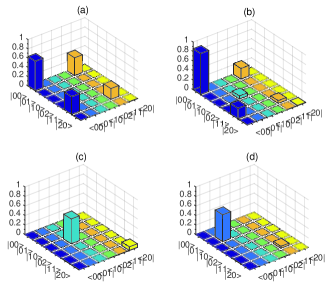
Figure 2: Fock matrix elements of four states in our considered subspace. (a) $\rho_{ab}^{\left(I\right)}$; (b) $\rho_{ab}^{\left(III-11\right)}$; (c) $\rho_{ab}^{\left(III-01\right)}$; (d) $\rho_{ab}^{\left(III-10\right)}$, with $r=0.7$, $\eta=0.2$, $T=0.7$. In Fig.2 (a), $p_{00,00}=0.63474$, $p_{11,11}=0.231845$ and $p_{00,11}=p_{11,00}=0.383616$; In Fig.2 (b), $p_{00,00}^{\left(11\right)}=0.861274$, $p_{10,10}^{\left(11\right)}=0.0629178$, $p_{11,11}^{\left(11\right)}=0.0575249$, $p_{20,20}^{\left(11\right)}=0.00459628$, and $p_{00,11}^{\left(11\right)}=p_{11,00}^{\left(11\right)}=0.222586$; In Fig.2 (c), $p_{10,10}^{\left(01\right)}=0.521865$, $p_{20,20}^{\left(01\right)}=0.0762466$; Fig.2 (d), $p_{01,01}^{\left(10\right)}=0.562993$, $p_{11,11}^{\left(10\right)}=0.0411278$.

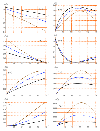
Figure 3: Population elements (a) $p_{00,00}^{\left(11\right)}$, (b) $p_{11,11}^{\left(11\right)}$, (c) $p_{10,10}^{\left(11\right)}$ and (d) $p_{20,20}^{\left(11\right)}$ in state $\rho_{ab}^{\left(III-11\right)}$ as a function of $\eta$ with $T=0.7$ (left) or as a function $T$ with $\eta=0.2$ (right). Here the black solid line, blue dashed line and brown dotdashed line are corresponding to $r=0.5$, $r=0.7$ and $r=1$, respectively.

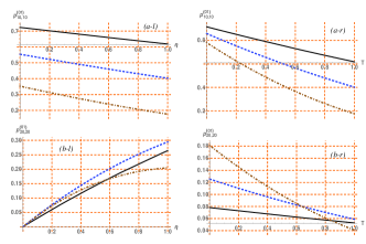
Figure 4: Population elements (a) $p_{10,10}^{\left(01\right)}$ and (b) $p_{20,20}^{\left(01\right)}$ in state $\rho_{ab}^{\left(III-01\right)}$ as a function of $\eta$ with $T=0.7$ (left) or as a function $T$ with $\eta=0.2$ (right). Here the black solid line, blue dashed line and brown dotdashed line are corresponding to $r=0.5$, $r=0.7$ and $r=1$, respectively.

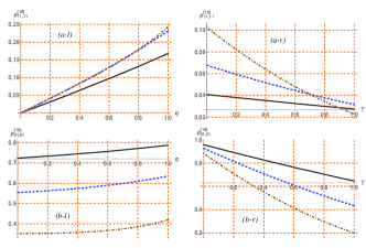
Figure 5: Population elements (a) $p_{01,01}^{\left(10\right)}$ and (b) $p_{11,11}^{\left(10\right)}$ in state $\rho_{ab}^{\left(III-10\right)}$ as a function of $\eta$ with $T=0.7$ (left) or as a function $T$ with $\eta=0.2$ (right). Here the black solid line, blue dashed line and brown dotdashed line are corresponding to $r=0.5$, $r=0.7$ and $r=1$, respectively.

V Conclusions and discussions

To summarize, we theoretically realized conditional operations to change the Fock matrix elements of the TMSVS. These operations include OPR, OPS and OPA. Everyone knows that the most prominent feature of the TMSVS is the twin-number field, which leads to the population and coherence components only from twin-Fock states. By employing three conditional operations, we have prepared three entangled resources from the original TMSVS. We obtain the analytical expressions of their Fock matrix elements and analyze the change in elements. In the finite subspace span $\left\{\left|00\right\rangle,\left|01\right\rangle,\left|10\right\rangle,\left|02\right\rangle,\left|11\right\rangle,\left|20\right\rangle\right\}$, we compare their population elements, as shown in Table VI. Compared with that the TMSVS only has the populations in $\left|00\right\rangle$ and $\left|11\right\rangle$, we find that (1) the populations in $\left|10\right\rangle$ and $\left|20\right\rangle$ have been added for the generated state after OPR; (2) the populations in $\left|00\right\rangle$ and $\left|11\right\rangle$ have been lost and the populations in $\left|10\right\rangle$ and $\left|20\right\rangle$ have been added for the generated state after OPS; (3) the population only in $\left|11\right\rangle$ has been remained and the population in $\left|01\right\rangle$ has been added for the generated state after OPA. The numerical results are shown in some figures.

Table 6: Population elements in Fock matrix of these states in subspace span $\left\{\left|00\right\rangle,\left|01\right\rangle,\left|10\right\rangle,\left|02\right\rangle,\left|11\right\rangle,\left|20\right\rangle\right\}$

Population	$\left|00\right\rangle$	$\left|01\right\rangle$	$\left|10\right\rangle$	$\left|02\right\rangle$	$\left|11\right\rangle$	$\left|20\right\rangle$
$\rho_{ab}^{\left(I\right)}$	$\surd$				$\surd$
$\rho_{ab}^{\left(III-11\right)}$	$\surd$		$\surd$		$\surd$	$\surd$
$\rho_{ab}^{\left(III-01\right)}$			$\surd$			$\surd$
$\rho_{ab}^{\left(III-10\right)}$		$\surd$			$\surd$

In fact, there are a lot of related works. It is instructive to compare our work with earlier related works. In order to improve figures of merit for a quantum state, researchers often propose different quantum strategies, for example, by applying the non-Gaussian operations (including photon addition, photon subtraction, superposition of photon addition and subtraction) on the original state. Of course, for a two-mode state such as the TMSVS, these strategies may be applied to one or both modes. For example, Bartley and Walmsley compare entanglement enhancement of the TMSVS after applying these non-Gaussian operations 11 . In addition, by means of quantum catalysis 26a or quantum scissors 26b , the entanglement properties of the TMSVS can also be enhanced in some parameter range. For example, our group has two related works in recent years. One is by employed local quantum catalysis on the TMSVS 10 , another is by quantum scissors 26c on the TMSVS. In fact, the OPR scheme in our work is related to the idea of Ulanov and co-workers who proposed to distill the TMSVS by using noiseless amplifiction 21 . By the way, the OPS scheme in our work is related to the idea of Kurochkin and co-workers who demonstrated entanglement distillation by applying photon annihilation on only one of the modes of the initial TMSVS 26d . Previous analyses of these processes have adopted different figures of merit to compare each protocol, for example teleportation fidelity, squeezing effect or entanglement entropy. Unlike previous works, in this paper, we pay our attention on the Fock matrix elements of the density operators for quantum states under investigation.

Quantum technology protocols exploit the unique properties of quantum systems to fulfill communication, computing and metrology tasks that are impossible, inefficient or intractable for classical systems. Perhaps it is because of the most prominent characteristic (eg. squeezing and entanglement), the TMSVS have become the most commonly used entangled resource of quantum technology 27 . However, as our new states induced from the TMSVS, they must have their own unique characteristic, which will become new entangled resources to require the needs of quantum technologies. The development of technologies allows promising real applications in quantum information processing, such as quantum teleportation 28 , quantum computation 29 and quantum communication 30 . It is believed that our generating states will be good entangled resources for future application. Our theoretical analyses will provide some information for further application and stimulate the design of experimental tests.

Appendix A: Loss formula in CF formalism

About the detailed derivation of this loss formula, one can refer to our previous work 25 . The loss can be modelled in a BS formalism. The input state $\rho_{in}$ can be expressed in the CF representation

$$\rho_{in}=\int\frac{d^{2}\alpha}{\pi}\chi_{in}\left(\alpha\right)D_{a}\left(-\alpha\right),$$ (A.1)

where $D_{a}\left(\alpha\right)$ is the displacement operator in mode $a$, and $\chi_{in}\left(\alpha\right)=$Tr$\left(\rho_{in}D_{a}\left(\alpha\right)\right)$ is the CF of the input state $\rho_{in}$. The output state $\rho_{out}$ can be expressed as

$$\rho_{out} =\int\frac{d^{2}\alpha}{\pi\left(1-\eta\right)}e^{-\frac{\eta}{2\left(1-\eta\right)}\left|\alpha\right|^{2}}\chi_{in}\left(\alpha\right)$$

$$\times D_{a}(-\frac{\alpha}{\sqrt{1-\eta}}),$$ (A.2)

or

$$\rho_{out} =\int\frac{d^{2}\alpha}{\pi}e^{-\frac{1}{2}\eta\left|\alpha\right|^{2}}\chi_{in}(\sqrt{1-\eta}\alpha)$$

$$\times D_{a}\left(-\alpha\right),$$ (A.3)

where $\eta$ is the loss factor. So, once the input CF $\chi_{in}\left(\alpha\right)$ is known, one can obtain the output optical field after the loss according to Eqs. (A.2) or (A.3).

Appendix B: Success probability of generating states

In order to ensure Tr$(\rho_{ab}^{\left(III\right)})=1$, we must calculate the success probability for every scheme. These success probabilities in derivative forms are given as follows, i.e.,

$$p_{d}^{\left(11\right)} =\Omega\left(1-\lambda^{2}\right)\frac{d^{4}}{dh_{2}dh_{1}ds_{2}ds_{1}}$$

$$e^{\Omega\left(1-T\right)[\lambda^{2}\left(1-\eta\right)h_{1}h_{2}+(1-\lambda^{2}\eta)s_{1}s_{2}]}$$

$$\times e^{\Omega(1-\lambda^{2})\sqrt{T}\left(s_{1}h_{2}+h_{1}s_{2}\right)}|_{s_{1}=s_{2}=h_{1}=h_{2}=0},$$ (B.1)

and

$$p_{d}^{\left(10\right)} =\Omega\left(1-\lambda^{2}\right)\frac{d^{2}}{ds_{2}ds_{1}}$$

$$e^{\Omega\left(1-T\right)(1-\lambda^{2}\eta)s_{1}s_{2}}|_{s_{1}=s_{2}=h_{1}=h_{2}=0},$$ (B.2)

as well as

$$p_{d}^{\left(01\right)} =\Omega\left(1-\lambda^{2}\right)\frac{d^{2}}{dh_{2}dh_{1}}$$

$$e^{\Omega\left(1-T\right)\lambda^{2}\left(1-\eta\right)h_{1}h_{2}}|_{s_{1}=s_{2}=h_{1}=h_{2}=0}.$$ (B.3)

References

• (1) Toninelli E, Ndagano B, Valles A, Sephton B, Nape I, Ambrosio A, Capasso F, Padgett M J, and Forbes A 2019 Concepts in quantum state tomography and classical implementation with intense light: a tutorial, Advances in Optics and Photonics 11 67
• (2) Lvovsky A I and Raymer M G 2009 Continuous-variable optical quantum-state tomography Rev. Mod. Phys. 81 299
• (3) Almarashia A M, Algarnia A, Alabouda F M, Abdel-Khalekb S, Berrada K 2019 Optical tomography for excited coherent states associated to deformed oscillators Results in Physics 14 102352
• (4) Gerry C C and Knight P 2005 Introductory Quantum Optics (Cambridge: Cambridge University Press)
• (5) Wilde M M 2013 Quantum Information Theory (Cambridge: Cambridge University Press)
• (6) El-Shahat T M, Abdel-Khalek S, Abdel-Aty M, Obada A S F 2003 Aspects on entropy squeezing of a two-level atom in a squeezed vacuum Chaos, Solitons & Fractals 18 289
• (7) El-Shahat T M, Abdel-Khalek S, Obada A S F 2005 Entropy squeezing of a driven two-level atom in a cavity with injected squeezed vacuum Chaos, Solitons & Fractals 26 1293
• (8) Takeda S, Mizuta T, Fuwa M, van Loock P, Furusawa A 2013 Deterministic quantum teleportation of photonic quantum bits by a hybrid technique Nature 500 315
• (9) Quesada N, Helt L G, Izaac J, Arrazola J M, Shahrokhshahi R, Myers C R, and Sabapathy K K 2019 Simulating realistic non-Gaussian state preparation Phys. Rev. A 100, 022341 (2019)
• (10) Abdel-Khalek S and Obada A S F 2009 The atomic Wehrl entropy of a V-type three-level atom interacting with two-mode squeezed vacuum state Journal of Russian Laser Research 30 146
• (11) Magana-Loaiza O S, de J Leon-Montiel R, Perez-Leija A, U’Ren A B, You C L, Busch K, Lita A E, Nam S W, Mirin R P and Gerrits T 2019 Multiphoton Quantum-State Engineering using conditional measurements arXiv: 1901.00122
• (12) Dakna M, Anhut T, Opatrny T, Knoll L and Welsch D G 1997 Generating Schrodinger cat-like states by means of conditional measurements on a beam splitter Phys. Rev. A 55 3184
• (13) Dakna M, Knoll L and Welsch D G 1998 Photon-added state preparation via conditional measurement on a beam splitter Opt. Commun. 145 309
• (14) Lvovsky A I and Mlynek J 2002 Quantum-Optical Catalysis: Generating Nonclassical States of Light by Means of Linear Optics Phys. Rev. Lett. 88 250401
• (15) Bartley T J, Donati G, Spring J B, Jin X M, Barbieri M, Datta A, Smith B J and Walmsley I A 2012 Multiphoton state engineering by heralded interference between single photons and coherent states Phys. Rev. A 86 043820
• (16) Xu X X 2015 Enhancing quantum entanglement and quantum teleportation for two-mode squeezed vacuum state by local quantum-optical catalysis Phys. Rev. A 92 012318
• (17) Bartley T J and Walmsley I 2015 Directly comparing entanglement-enhancing non-Gaussian operations New J. Phys. 17 023038
• (18) Fiurasek J 2009 Engineering quantum operations on traveling light beams by multiple photon addition and subtraction Phys. Rev. A 80 053822
• (19) Neergaard-Nielsen J S, Nielsen B M, Hettich C, Molmer K and Polzik E S 2006 Generation of a superposition of odd photon number states for quantum information networks Phys. Rev. Lett. 97 083604
• (20) Zavatta A, Viciani S and Bellini M 2004 Quantum-to-classical transition with single-photon-added coherent states of light Science 306 660
• (21) Sabapathy K K and Winter A 2017 Non-Gaussian operations on bosonic modes of light: Photon-added Gaussian channels Phys. Rev. A 95 062309
• (22) Ourjoumtsev A, Dantan A, Tualle-Brouri R and Grangier P 2007 Increasing entanglement between Gaussian states by coherent photon subtraction Phys. Rev. Lett. 98 030502
• (23) Navarrete-Benlloch C, Garcia-Patron R, Shapiro J H and Cerf N J 2012 Enhancing quantum entanglement by photon addition and subtraction Phys. Rev. A 86 012328
• (24) Olivares S, Paris M G A and Bonifacio R 2003 Teleportation improvement by inconclusive photon subtraction Phys. Rev. A 67 032314
• (25) Opatrny T, Kurizki G and Welsch D G 2000 Improvement on teleporation of continuous variables by photon subtraction via conditional measurement Phys. Rev. A 61 032302
• (26) Micuda M, Straka I, Mikova M, Dusek M, Cerf N J, Fiurasek J and Jezek M 2012 Noiseless loss suppression in quantum optical communication Phys. Rev. Lett. 109 180503
• (27) Ulanov A E, Fedorov L A, Pushkina A A, Kurochkin Y V, Ralph T C and Lvovsky A I 2015 Undoing the effect of loss on quantum entanglement Nat. Photon. 9 764
• (28) Ulanov A E, Fedorov I A, Sychev D, Grangier P and Lvovsky A I 2016 Loss-tolerant state engineering for quantum-enhanced metrology via the reserse Hong-Ou-Mandel effect Nat. Commun. 7 11925
• (29) Adesso G, Dell’Anno F, De Siena S, Illuminati F and Souza L A M 2009 Optimal estimation of losses at the ultimate quantum limit with non-Gaussian states Phys. Rev. A 79 040305
• (30) Scully M O and Zubairy M S 1997 Quantum Optics (Cambridge: Cambridge University Press)
• (31) Xu X X and Yuan H C 2017 Some Evolution formulas on the optical fields propagation in realistic environments Int. J. Theor. Phys. 56 791
• (32) Xu X X and Yuan H C 2016 Generating single-photon catalyzed coherent states with quantum-optical catalysis Phys. Lett. A 380 2342
• (33) Lvovsky A I and Mlynek J 2002 Quantum-optical catalysis: generating nonclassical states of light by means of linear optics Phys. Rev. Lett. 88 250401
• (34) Pegg D, Phillips L and Barnett S 1998 Optical state truncation by projection synthesis Phys. Rev. Lett. 81 1604
• (35) Xu X X, Hu L Y, Liao Z Y 2018 Improvement of entanglement via quantum scissors J. Opt. Soc. Am. B 35 010174
• (36) Kurochkin Y, Prasad A S and Lvovsky A I 2014 Distillation of the two-mode squeezed state Phys. Rev. Lett. 112 070402
• (37) Takeda S, Fuwa M, van Loock P and Furusawa A 2015 Entanglement swapping between discrete and continuous variables Phys. Rev. Lett. 114 100501
• (38) Bennett C H, Brassard G, Crepeau C, Jozsa R, Peres A and Wootters W K 1993 Teleporting an unknown quantum state via dual classical and Einstein-Podolsky-Rosen channels Phys. Rev. Lett. 70 1895
• (39) Lloyd S and Braunstein S L 1999 Quantum compution over continuous variables Phys. Rev. Lett. 82 1784
• (40) Scarani R, Bechmann-Pasquinucci H, Cerf N J, Dusek M, Lutkenhaus N and Peev M 2009 The security of practical quantum key distribution Rev. Mod. Phys. 81 1301