On Tree-based Methods for Similarity Learning

Abstract

In many situations, the choice of an adequate similarity measure or metric on the feature space dramatically determines the performance of machine learning methods. Building automatically such measures is the specific purpose of metric/similarity learning. In [21], similarity learning is formulated as a pairwise bipartite ranking problem: ideally, the larger the probability that two observations in the feature space belong to the same class (or share the same label), the higher the similarity measure between them. From this perspective, the ${\rm ROC}$ curve is an appropriate performance criterion and it is the goal of this article to extend recursive tree-based ${\rm ROC}$ optimization techniques in order to propose efficient similarity learning algorithms. The validity of such iterative partitioning procedures in the pairwise setting is established by means of results pertaining to the theory of $U$-processes and from a practical angle, it is discussed at length how to implement them by means of splitting rules specifically tailored to the similarity learning task. Beyond these theoretical/methodological contributions, numerical experiments are displayed and provide strong empirical evidence of the performance of the algorithmic approaches we propose.

Keywords: Metric-Learning $\cdot$ Rate Bound Analysis $\cdot$ Similarity Learning $\cdot$ Tree-based Algorithms $\cdot$ $U$-processes.

1 Introduction

Similarity functions are ubiquitous in machine learning, they are the essential ingredient of nearest neighbor rules in classification/regression or K-means/medoids clustering methods for instance and crucially determine their performance when applied to major problems such as biometric identification or recommending system design. The goal of learning automatically from data a similarity function or a metric has been formulated in various ways, depending on the type of similarity feedback available (e.g. labels, preferences), see [15, 1, 5, 14, 20]. A dedicated literature has recently emerged, devoted to this class of problems that is referred to as similarity-learning or metric-learning and is now receiving much attention, see e.g. [2] or [16] and the references therein. A popular framework, akin to that of multi-class classification, stipulates that pairwise similarity judgments can be directly deduced from observed class labels: a positive label is assigned to pairs formed of observations in the same class, while a negative label is assigned to those lying in different classes. In this context, similarity learning has been recently expressed as a pairwise bipartite ranking problem in [21], the task consisting in learning a similarity function that ranks the elements of a database by decreasing order of the posterior probability that they share the same label with some arbitrary query data point, as it is the case in important applications. In biometric identification (see e.g. [12]), the identity claimed by an individual is checked by matching her biometric information, a photo or fingerprints taken at an airport for instance, with those of authorized people gathered in a data repository of reference (e.g. passport photos or fingerprints). Based on a given similarity function and a fixed threshold value, the elements of the database are sorted by decreasing order of similarity score with the query and those whose score exceeds the threshold specified form the collection of matching elements. The ${\rm ROC}$ curve of a similarity function, i.e. the plot of the false positive rate vs the true positive rate as the threshold varies, appears in this situation as a natural (functional) performance measure. Whereas several approaches have been proposed to optimize a statistical counterpart of its scalar summary, the ${\rm AUC}$ criterion (${\rm AUC}$ standing for Area Under the ${\rm ROC}$ Curve), see [18, 11], it is pointed out in [21] that more local criteria must be considered in practice: ideally, the true positive rate should be maximized under the constraint that the false positive rate remains below a fixed level, usually specified in advance on the basis of operational constraints (see [12, 13] in the case of biometric applications). If the generalization ability of solutions of empirical versions of such pointwise ${\rm ROC}$ optimization problems (and the situations where fast learning rates are achievable as well) has been investigated at length in [21], it is very difficult to solve in practice these constrained, generally nonconvex, optimization problems. It is precisely the goal of the present paper to address this algorithmic issue. Our approach builds on an iterative ${\rm ROC}$ optimization method, referred to as TreeRank, that has been proposed in [8] (see also [7] as well as [6] for an ensemble learning technique based on this method) and investigated at length in the standard (non pairwise) bipartite ranking setting. In this article, we establish statistical guarantees for the validity of the TreeRank methodology, when extended to the similarity learning framework (i.e. pairwise bipartite ranking), in the form of generalization rate bounds related to the $\sup$ norm in the ${\rm ROC}$ space and discuss issues related to its practical implementation. In particular, the splitting rules recursively implemented in the variant we propose are specifically tailored to the similarity learning task and produce symmetric tree-based scoring rules that may thus serve as similarity functions. Numerical experiments based on synthetic and real data are also presented here, providing strong empirical evidence of the relevance of this approach for similarity learning.
The paper is organized as follows. The rigorous formulation of similarity learning as pairwise bipartite ranking is briefly recalled in section 2, together with the main principles underlying the TreeRank algorithm for ${\rm ROC}$ optimization. In section 3, theoretical results proving the validity of the TreeRank method in the pairwise setup are stated and practical implementation issues are also discussed. Section 4 displays illustrative experimental results.

2 Background and Preliminaries

We start with recalling key concepts of similarity learning and its natural connection with ${\rm ROC}$ analysis and next briefly describe the algorithmic principles underlying the TreeRank methodology. Throughout the article, the Dirac mass at any point $x$ is denoted by $\delta_{x}$, the indicator function of any event $\mathcal{E}$ by $\mathbb{I}\{\mathcal{E}\}$, and the pseudo-inverse of any cdf $F(u)$ on $\mathbb{R}$ by $F^{-1}(t)=\inf\{v\in\mathbb{R}:\;F(v)\geq t\}$.

2.1 Similarity Learning as Pairwise Bipartite Ranking

We place ourselves in the probabilistic setup of multi-class classification here: $Y$ is a random label, taking its values in $\{1,\;\ldots,\;K\}$ with $K\geq 1$ say, and $X$ is a random vector defined on the same probability space, valued in a feature space $\mathcal{X}\subset\mathbb{R}^{d}$ with $d\geq 1$ and modelling some information hopefully useful to predict $Y$. The marginal distribution of $X$ is denoted by $\mu(dx)$, while the prior/posterior probabilities are $p_{k}=\mathbb{P}\{Y=k\}$ and $\eta_{k}(X)=\mathbb{P}\{Y=k\mid X\}$, $k=1,\;\ldots,\;K$. The conditional distribution of the r.v. $X$ given $Y=k$ is denoted by $\mu_{k}$. The distribution $P$ of the generic pair $(X,Y)$ is entirely characterized by $(\mu,\;(\eta_{1},\;\ldots,\;\eta_{K}))$. Equipped with these notations, we have $\mu=\sum_{k}p_{k}\mu_{k}$ and $p_{k}=\int_{\mathcal{X}}\eta_{k}(x)\mu(dx)$ for $k\in\{1,\;\ldots,\;K\}$. In a nutshell, the goal pursued in this similarity learning framework is to learn from a training dataset $\mathcal{D}_{n}=\{(X_{1},Y_{1}),\;\ldots,\;(X_{n},Y_{n})\}$ composed of independent observations with distribution $P$ a similarity (scoring) function, that is a measurable symmetric function $s:\mathcal{X}^{2}\to\mathbb{R}_{+}$ (i.e. $\forall(x,x^{\prime})\in\mathcal{X}^{2}$, $s(x,x^{\prime})=s(x^{\prime},x)$) such that, given an independent copy $(X^{\prime},Y^{\prime})$ of $(X,Y)$, the larger the similarity score between the input observations $X$ and $X^{\prime}$, the higher the probability that they share the same label (i.e. that $Y=Y^{\prime}$) should be. We denote by $\mathcal{S}$ the ensemble of all similarity functions.
Optimal rules. Given this informal objective, the set of optimal similarity functions is obviously formed of strictly increasing transforms of the (symmetric) posterior probability $\eta(x,x^{\prime})=\mathbb{P}\{Y=Y^{\prime}\mid(X,X^{\prime})=(x,x^{\prime})\}$, namely

$$\mathcal{S}^{*}=\{T\circ\eta:\;\;T:Im(\eta)\to\mathbb{R}_{+}\text{ borelian, strictly increasing}\},$$

denoting by $Im(\eta)$ the support of the r.v. $\eta(X,X^{\prime})=\sum_{k}\eta_{k}(X)\eta_{k}(X^{\prime})$. A similarity function $s^{*}\in\mathcal{S}^{*}$ defines the optimal preorder $\preceq^{*}$ on the product space $\mathcal{X}\times\mathcal{X}$: for all $(x_{1},x_{2},x_{3},x_{4})\in\mathcal{X}^{4}$, $x_{1}$ and $x_{2}$ are more similar to each other than $x_{3}$ and $x_{4}$ iff $\eta(x_{1},x_{2})\geq\eta(x_{3},x_{4})$, and one then writes $(x_{3},x_{4})\preceq^{*}(x_{1},x_{2})$. For any query $x\in\mathcal{X}$, $s^{*}$ also defines a preorder $\preceq^{*}_{x}$ on the input space $\mathcal{X}$, that enables us to rank optimally all possible observations by increasing degree of similarity to $x$: for any $(x_{1},x_{2})\in\mathcal{X}^{2}$, $x_{1}$ is more similar to $x$ than $x_{2}$ (one writes $x_{2}\preceq^{*}_{x}x_{1}$) iff $(x,x_{2})\preceq^{*}(x,x_{1})$, that is $\eta(x,x_{2})\leq\eta(x,x_{1})$.
Pointwise ${\rm ROC}$ curve optimization. As highlighted in [21], similarity learning can be formulated as a bipartite ranking problem on the product space $\mathcal{X}\times\mathcal{X}$ where, given two independent realizations $(X,Y)$ and $(X^{\prime},Y^{\prime})$ of $P$, the input r.v. is the pair $(X,X^{\prime})$ and the binary label is $Z=2\mathbb{I}\{Y=Y^{\prime}\}-1$, see e.g. [9]. In bipartite ranking, the gold standard by which the performance of a scoring function $s$ is measured is the ${\rm ROC}$ curve (see e.g. [10] for an account of ${\rm ROC}$ analysis and its applications.): one evaluates how close the preorder induced by $s$ to $\preceq^{*}$ is by plotting the parametric curve $t\in\mathbb{R}_{+}\mapsto(F_{s,-}(t),F_{s,+}(t))$, where

$$F_{s,-}(t)=\mathbb{P}\{s(X,X^{\prime})>t\mid Z=-1\},\;F_{s,+}(t)=\mathbb{P}\{s(X,X^{\prime})>t\mid Z=+1\},$$

where possible jumps are connected by line segments. This P-P plot is referred to as the ${\rm ROC}$ curve of $s(x,x^{\prime})$ and can be viewed as the graph of a continuous function $\alpha\in(0,1)\mapsto{\rm ROC}_{s}(\alpha)$, where ${\rm ROC}_{s}(\alpha)=F_{s,+}\circ F_{s,-}^{-1}(\alpha)$ at any point $\alpha\in(0,1)$ such that $F_{s,-}\circ F_{s,-}^{-1}(\alpha)=\alpha$. The curve ${\rm ROC}_{s}$ informs us about the capacity of $s$ to discriminate between pairs with same labels and pairs with different labels: the stochastically larger than $F_{s,-}$ the distribution $F_{s,+}$, the higher ${\rm ROC}_{s}$. It corresponds to the type I error vs power plot (false positive rate vs true positive rate) of the statistical test $\mathbb{I}\{s(X,X^{\prime})>t\}$ when the null hypothesis stipulates that the labels of $X$ and $X^{\prime}$ are different (i.e. $Y\neq Y^{\prime}$) and defines a partial preorder on the set $\mathcal{S}$: one says that a similarity function $s_{1}$ is more accurate than another one $s_{2}$ when, for all $\alpha\in(0,1)$, ${\rm ROC}_{s_{2}}(\alpha)\leq{\rm ROC}_{s_{1}}(\alpha)$. The optimality of the elements of $\mathcal{S}^{*}$ w.r.t. this partial preorder immediately results from a classic Neyman-Pearson argument: $\forall(s,s^{*})\in\mathcal{S}\times\mathcal{S}^{*}$, ${\rm ROC}_{s}(\alpha)\leq{\rm ROC}_{s^{*}}(\alpha)={\rm ROC}_{\eta}(\alpha):={\rm ROC}^{*}(\alpha)$ for all $\alpha\in(0,1)$. For simplicity, we assume here that the conditional cdf of $\eta(X,X^{\prime})$ given $Z=-1$ is invertible. The accuracy of any $s\in\mathcal{S}$ can be measured by:

$$D_{p}(s,s^{*})=||{\rm ROC}_{s}-{\rm ROC}^{*}||_{p},$$ (1)

where $s^{*}\in\mathcal{S}^{*}$ and $p\in[1,+\infty]$. When $p=1$, one may write $D_{1}(s,s^{*})={\rm AUC}^{*}-{\rm AUC}(s)$, where ${\rm AUC}(s)=\int_{\alpha=0}^{1}{\rm ROC}_{s}(\alpha)d\alpha$ is the Area Under the ${\rm ROC}$ Curve (${\rm AUC}$ in short) and ${\rm AUC}^{*}={\rm AUC}(\eta)$ is the maximum ${\rm AUC}$. Minimizing $D_{1}(s,s^{*})$ boils down thus to maximizing the ${\rm ROC}$ summary ${\rm AUC}(s)$, whose popularity arises from its interpretation as the rate of concording pairs:

$${\rm AUC}(s)=\mathbb{P}\left\{s(X_{1},X_{1}^{\prime})<s(X_{2},X_{2}^{\prime})\mid(Z_{1},Z_{2})=(-1,+1)\right\}\\ +\frac{1}{2}\mathbb{P}\left\{s(X_{1},X_{1}^{\prime})=s(X_{2},X_{2}^{\prime})\mid(Z_{1},Z_{2})=(-1,+1)\right\},$$

where $((X_{1},X^{\prime}_{1}),Z_{1})$ and $((X_{2},X_{2}^{\prime}),Z_{2})$ denote independent copies of $((X,X^{\prime}),Z)$. A simple empirical counterpart of ${\rm AUC}(s)$ can be derived from this formula, paving the way for the implementation of ”empirical risk minimization” strategies, see [9] (the algorithms proposed to optimize the ${\rm AUC}$ criterion or surrogate performance measures are too numerous to be listed exhaustively here). However, as mentioned precedingly, in many applications, one is interested in finding a similarity function that optimizes the ${\rm ROC}$ curve at specific points $\alpha\in(0,1)$. The superlevel sets of similarity functions in $\mathcal{S}^{*}$ define the solutions of pointwise ${\rm ROC}$ optimization problems in this context. In the above framework, it indeed follows from Neyman Pearson’s lemma that the test statistic of type I error less than $\alpha$ with maximum power is the indicator function of the set $\mathcal{R}^{*}_{\alpha}=\{(x,x^{\prime})\in\mathcal{X}^{2}:\;\eta(x,x^{\prime})\geq Q^{*}_{\alpha}\}$, where $Q^{*}_{\alpha}$ is the conditional quantile of the r.v. $\eta(X,X^{\prime})$ given $Z=-1$ at level $1-\alpha$. Considering similarity functions that are bounded by $1$ only, it corresponds to the unique solution of the problem:

$$\max_{{\scriptsize\begin{array}[]{c}s:\mathcal{X}^{2}\rightarrow[0,1],\\ \text{ borelian}\end{array}}}\mathbb{E}[s(X,X^{\prime})\mid Z=+1]\quad\text{subject to}\quad\mathbb{E}[s(X,X^{\prime})\mid Z=-1]\leq\alpha.$$

Though its formulation is natural, this constrained optimization problem is very difficult to solve in practice, as discussed at length in [21]. This suggests the extension to the similarity ranking framework of the TreeRank approach for ${\rm ROC}$ optimization (see [8] and [7]), recalled below. Indeed, in the standard (non pairwise) statistical learning setup for bipartite ranking, whose probabilistic framework is the same as that of binary classification and stipulates that training data are i.i.d. labeled observations, this recursive technique builds (piecewise constant) scoring functions $s$, whose accuracy can be guaranteed in terms of $\sup$ norm (i.e. for which $D_{\infty}(s,s^{*})$ can be controlled) and it is the essential purpose of the subsequent analysis to prove that this remains true when the training observations are of the form $\{((X_{i},X_{j}),\;Z_{i,j}):\;1\leq i<j\leq n\}$, where $Z_{i,j}=2\mathbb{I}\{Y_{i}=Y_{j}\}-1$ for $1\leq i<j\leq n$, and are thus far from being independent. Regarding its implementation, attention should be paid to the fact that the splitting rules for recursive partitioning of the space $\mathcal{X}\times\mathcal{X}$ must ensure that the decision functions produced by the algorithm fulfill the symmetric property.

2.2 Recursive ${\rm ROC}$ Curve Optimization - The TreeRank Algorithm

Because they offer a visual model summary in the form of an easily interpretable binary tree graph, decision trees remain very popular among practicioners, see e.g. [4] or [19]. In general, predictions are computed through a hierarchical combination of elementary rules comparing the value taken by a (quantitative) component of the input information (the split variable) to a certain threshold (the split value). In contrast to (supervised) learning problems such as classification/regression, which are of local nature, predictive rules for a global problem such as similarity learning cannot be described by a simple (tree-structured) partition of $\mathcal{X}\times\mathcal{X}$: the (symmetric) cells corresponding to the terminal leaves of the binary decision tree must be sorted in order to define a similarity function.

Similarity Trees. We define a similarity tree as a binary tree whose leaves all correspond to symmetric subsets $\mathcal{C}$ of the product space $\mathcal{X}\times\mathcal{X}$ (i.e. $\forall(x,x^{\prime})\in\mathcal{X}^{2}$; $(x,x^{\prime})\in\mathcal{C}\Leftrightarrow(x^{\prime},x)\in\mathcal{C}$) and is equipped with a ’left-to-right’ orientation, that defines a tree-structured collection of similarity functions. Incidentally, the symmetry property makes it a specific ranking tree, using the terminology introduced in [8]. The root node of a tree $\mathcal{T}_{J}$ of depth $J\geq 0$ corresponds to the whole space $\mathcal{X}\times\mathcal{X}$: $\mathcal{C}_{0,0}=\mathcal{X}^{2}$, while each internal node $(j,k)$ with $j<J$ and $k\in\{0,\;\ldots,\;2^{j}-1\}$ represents a subset $\mathcal{C}_{j,k}\subset\mathcal{X}^{2}$, whose left and right siblings respectively correspond to (symmetric) disjoint subsets $\mathcal{C}_{j+1,2k}$ and $\mathcal{C}_{j+1,2k+1}$ such that $\mathcal{C}_{j,k}=\mathcal{C}_{j+1,2k}\cup\mathcal{C}_{j+1,2k+1}$. Equipped with the left-to-right orientation, any subtree $\mathcal{T}\subset\mathcal{T}_{J}$ defines a preorder on $\mathcal{X}^{2}$: the degree of similarity being the same for all pairs $(x,x^{\prime})$ lying in the same terminal cell of $\mathcal{T}$. The similarity function related to the oriented tree $\mathcal{T}$ can be written as:

$$\forall(x,x^{\prime})\in\mathcal{X}^{2},\;\;s_{\mathcal{T}}(x,x^{\prime})=\sum_{\mathcal{C}_{j,k}:\text{ terminal leaf of }\mathcal{T}}2^{J}\left(1-\frac{k}{2^{j}}\right)\cdot\mathbb{I}\{(x,x^{\prime})\in\mathcal{C}_{j,k}\}.$$

Observe that its symmetry results from that of the $\mathcal{C}_{j,k}$’s.  The ${\rm ROC}$ curve of the similarity function $s_{\mathcal{T}}(x,x^{\prime})$ is the piecewise linear curve connecting the knots:

$$(0,0)\text{ and }\;\left(\sum_{l=0}^{k}F_{-}(\mathcal{C}_{j,l}),\;\sum_{l=0}^{k}F_{+}(\mathcal{C}_{j,l})\right)\text{ for all terminal leaf }\mathcal{C}_{j,k}\text{ of }\mathcal{T},$$

denoting by $F_{\sigma}$ the conditional distribution of $(X,X^{\prime})$ given $Z=\sigma 1$, $\sigma\in\{-.\;+\}$. Setting $p_{+}=\mathbb{P}\{Z=+1\}=\sum_{k}p_{k}^{2}$, we have $F_{+}=(1/p_{+})\sum_{k}p_{k}^{2}\cdot\mu_{k}\otimes\mu_{k}$ and $F_{-}=(1/(1-p_{+}))\sum_{k\neq l}p_{k}p_{l}\cdot\mu_{k}\otimes\mu_{l}$. A statistical version can be computed by replacing the $F_{\sigma}(\mathcal{C}_{j,l})$’s by their empirical counterpart.
Growing the Similarity Tree. The TreeRank algorithm, a bipartite ranking technique optimizing the ${\rm ROC}$ curve in a recursive fashion, has been introduced in [8] and its properties have been investigated in [7] at length. Its output consists of a tree-structured scoring rule (2.2) with a ${\rm ROC}$ curve that can be viewed as a piecewise linear approximation of ${\rm ROC}^{*}$ obtained by a Finite Element Method with implicit scheme and is proved to be nearly optimal in the $D_{1}$ sense under mild assumptions. The growing stage is performed as follows. At the root, one starts with a constant similarity function $s_{1}(x,x^{\prime})=\mathbb{I}\{(x,x^{\prime})\in\mathcal{C}_{0,0}\}\equiv 1$ and after $m=2^{j}+k$ iterations, $0\leq k<2^{j}$, the current similarity function is

$$s_{m}(x,x^{\prime})=\sum_{l=0}^{2k-1}(m-l)\cdot\mathbb{I}\{(x,x^{\prime})\in\mathcal{C}_{j+1,l}\}+\sum_{l=k}^{2^{j}-1}(m-k-l)\cdot\mathbb{I}\{(x,x^{\prime})\in\mathcal{C}_{j,l}\}$$

and the cell $\mathcal{C}_{j,k}$ is split so as to form a refined version of the similarity function,

$$s_{m+1}(x,x^{\prime})=\sum_{l=0}^{2k}(m-l)\cdot\mathbb{I}\{(x,x^{\prime})\in\mathcal{C}_{j+1,l}\}+\sum_{l=k+1}^{2^{j}-1}(m-k-l)\cdot\mathbb{I}\{(x,x^{\prime})\in\mathcal{C}_{j,l}\}$$

namely, with maximum (empirical) ${\rm AUC}$. Therefore, it happens that this problem boils down to solve a cost-sensitive binary classification problem on the set $\mathcal{C}_{j,k}$, see subsection 3.3 in [7]. Indeed, one may write the ${\rm AUC}$ increment as

$${\rm AUC}(s_{m+1})-{\rm AUC}(s_{m})=\frac{1}{2}F_{-}(\mathcal{C}_{j,k})F_{+}(\mathcal{C}_{j,k})\times(1-\Lambda(\mathcal{C}_{j+1,2k}\mid\mathcal{C}_{j,k})),$$

$$\text{where }\Lambda(\mathcal{C}_{j+1,2k}\mid\mathcal{C}_{j,k})\overset{def}{=}F_{+}(\mathcal{C}_{j,k}\setminus\mathcal{C}_{j+1,2k})/F_{+}(\mathcal{C}_{j,k})+F_{-}(\mathcal{C}_{j+1,2k})/F_{-}(\mathcal{C}_{j,k}).$$

Setting $p=F_{+}(\mathcal{C}_{j,k})/(F_{-}(\mathcal{C}_{j,k})+F_{+}(\mathcal{C}_{j,k}))$, the crucial point of the TreeRank approach is that the quantity $2p(1-p)\Lambda(\mathcal{C}_{j+1,2k}\mid\mathcal{C}_{j,k})$ can be interpreted as the cost-sensitive error of a classifier on $\mathcal{C}_{j,k}$ predicting positive label for any pair lying in $\mathcal{C}_{j+1,2k}$ and negative label fo all pairs in $\mathcal{C}_{j,k}\setminus\mathcal{C}_{j+1,2k}$ with cost $p$ (respectively, $1-p$) assigned to the error consisting in predicting label $+1$ given $Z=-1$ (resp., label $-1$ given $Z=+1$), balancing thus the two types of error. Hence, at each iteration of the similarity tree growing stage, the TreeRank algorithm calls a cost-sensitive binary classification algorithm, termed LeafRank, in order to solve a statistical version of the problem above (replacing the theoretical probabilities involved by their empirical counterparts) and split $\mathcal{C}_{j,k}$ into $\mathcal{C}_{j+1,2k}$ and $\mathcal{C}_{j+1,2k+1}$. As described at length in [7], one may use cost-sensitive versions of celebrated binary classification algorithms such as CART or SVM for instance as LeafRank procedure, the performance depending on their ability to capture the geometry of the level sets $\mathcal{R}^{*}_{\alpha}$ of the posterior probability $\eta(x,x^{\prime})$. As highlighted above, in order to apply the TreeRank approach to similarity learning, a crucial feature the LeafRank procedure implemented must have is the capacity to split a region in subsets that are both stable under the reflection $(x,x^{\prime})\in\mathcal{X}^{2}\mapsto(x^{\prime},x)$. This point is discussed in the next section. Rate bounds for the TreeRank method in the $\sup$ norm sense are also established therein in the statistical framework of similarity learning, when the set of training examples $\{((X_{i},X_{j}),\;Z_{i,j}\}_{i<j}$ is composed of non independent observations with binary labels, formed from the original multi-class classification dataset $\mathcal{D}_{n}$.

3 A Tree-Based Approach to Similarity Learning

We now investigate how the TreeRank method for ${\rm ROC}$ optimization recalled in the preceding section can be extended to the framework of similarity-learning and next establish learning rates in $\sup$ norm in this context.

3.1 A Similarity-Learning Version of TreeRank

From a statistical perspective, a learning algorithm can be derived from the recursive approximation procedure recalled in the previous section, simply by replacing the quantities $F_{\sigma}(\mathcal{C})$, $\sigma\in\{-,\;+\}$ and $\mathcal{C}\subset\mathcal{X}\times\mathcal{X}$ borelian, by their empirical counterparts based on the dataset $\mathcal{D}_{n}$:

$$\widehat{F}_{\sigma,n}(\mathcal{C})=\frac{1}{n_{\sigma}}\sum_{i<j}\mathbb{I}\{(X_{i},X_{j})\in\mathcal{C},\;Z_{i,j}=\sigma 1\},$$ (2)

with $n_{\sigma}=(2/(n(n-1)))\sum_{i<j}\mathbb{I}\{Z_{i,j}=\sigma 1\}$. Observe incidentally that the quantities (2) are by no means i.i.d. averages, but take the form of ratios of $U$-statistics of degree two (i.e. averages over pairs of observations, cf [17]), see section 3 in [21]. For this reason, a specific rate bound analysis (ignoring bias issues) guaranteeing the accuracy of the TreeRank approach in the similarity learning framework is carried out in the next subsection.

The Similarity TreeRank Algorithm Input. Maximal depth $D\geq 1$ of the similarity tree, class $\mathcal{A}$ of measurable and symmetric subsets of $\mathcal{X}\times\mathcal{X}$, training dataset $\mathcal{D}_{n}=\{(X_{1},Y_{1}),\;\ldots,\;(X_{n},Y_{n})\}$. 1. (Initialization.) Set $\mathcal{C}_{0,0}=\mathcal{X}\times\mathcal{X}$, $\alpha_{d,0}=\beta_{d,0}=0$ and $\alpha_{d,2^{d}}=\beta_{d,2^{d}}=1$ for all $d\geq 0$. 2. (Iterations.) For $d=0,\;\ldots,\;D-1$ and $k=0,\;\ldots,\;2^{d}-1$: (a) (Optimization step.) Set the entropic measure: $\displaystyle\Lambda_{d,k+1}(\mathcal{C})$ $\displaystyle=$ $\displaystyle(\alpha_{d,k+1}-\alpha_{d,k})\widehat{F}_{+,n}(\mathcal{C})-(\beta_{d,k+1}-\beta_{d,k})\widehat{F}_{-,n}(\mathcal{C})~{}.$ Find the best subset $\mathcal{C}_{d+1,2k}$ of the cell $\mathcal{C}_{d,k}$ in the ${\rm AUC}$ sense: $$\mathcal{C}_{d+1,2k}=\mathop{\rm arg\,max}_{\mathcal{C}\in\mathcal{A},~{}\mathcal{C}\subset\mathcal{C}_{d,k}}\widehat{\Lambda}_{d,k+1}(\mathcal{C})~{}.$$ (3) Then, set $\mathcal{C}_{d+1,2k+1}=\mathcal{C}_{d,k}\setminus\mathcal{C}_{d+1,2k}$. (b) (Update.) Set $$\alpha_{d+1,2k+1}=\alpha_{d,k}+\widehat{F}_{-,n}(\mathcal{C}_{d+1,2k}),\;\beta_{d+1,2k+1}=\beta_{d,k}+\widehat{F}_{+,n}(\mathcal{C}_{d+1,2k})$$ $$\text{and }\alpha_{d+1,2k+2}=\alpha_{d,k+1},\;\beta_{d+1,2k+2}=\beta_{d,k+1}~{}.$$ 3. (Output.) After $D$ iterations, get the piecewise constant similarity function: $$s_{D}(x,x^{\prime})=\sum_{k=0}^{2^{D}-1}(2^{D}-k)~{}\mathbb{I}\{(x,x^{\prime})\in\mathcal{C}_{D,k}\},$$ (4) together with an estimate of the curve ${\rm ROC}(s_{D},.)$, namely the broken line $\widehat{{\rm ROC}}(s_{D},.)$ that connects the knots $\{(\alpha_{D,k},\beta_{D,k}):\;k=0,\ldots,2^{D}\}$, and the following estimate of ${\rm AUC}(s_{D})$: $\displaystyle\widehat{{\rm AUC}}(s_{D})$ $\displaystyle=$ $\displaystyle\int_{\alpha=0}^{1}\widehat{{\rm ROC}}(s_{D},\alpha)d\alpha=\frac{1}{2}+\frac{1}{2}\sum_{k=0}^{2^{D-1}-1}\widehat{\Lambda}_{D-1,k+1}(\mathcal{C}_{D,2k}).$

The symmetry property of the function (4) output by the learning algorithm is directly inherited from that of the candidate subsets $\mathcal{C}\in\mathcal{A}$ of the product space $\mathcal{X}\times\mathcal{X}$ among which the $\mathcal{C}_{d,k}$’s are selected. We new explain at length how to perform the optimization step (3) in practice in the similarity learning context.
Splitting for Similarity Learning. As recalled in subsection 2.2, solving (3) boils down to finding the best classifier on $\mathcal{C}_{d,k}\subset\mathcal{X}^{2}$ of the form

$$g_{\mathcal{C}\mid\mathcal{C}_{d,k}}(x,x^{\prime})=\mathbb{I}\{(x,x^{\prime})\in\mathcal{C}\}-\mathbb{I}\{(x,x^{\prime})\in\mathcal{C}\setminus\mathcal{C}_{d,k}\}\;\text{ with }\mathcal{C}\subset\mathcal{C}_{d,k},\;\;\mathcal{C}\in\mathcal{A},$$

in the empirical ${\rm AUC}$ sense, that is to say that minimizing a statistical version of the cost-sensitive classification error based on $\{((X_{i},X_{j}),\;Z_{i,j}):\;\;1\leq i<j\leq n,\;(X_{i},X_{j})\in\mathcal{C}_{d,k}\}$

$$\Lambda(\mathcal{C}\mid\mathcal{C}_{d,k})=\frac{\mathbb{P}\{g_{\mathcal{C}\mid\mathcal{C}_{d,k}}(X,X^{\prime})=1\mid Z=-1\}}{\mathbb{P}\{(X,X^{\prime})\in\mathcal{C}_{d,k}\mid Z=-1\}}+\frac{\mathbb{P}\{g_{\mathcal{C}\mid\mathcal{C}_{d,k}}(X,X^{\prime})=-1\mid Z=1\}}{\mathbb{P}\{(X,X^{\prime})\in\mathcal{C}_{d,k}\mid Z=1\}}.$$

Notice that, equipped with the notations previously introduced, the statistical version of $\Lambda(\mathcal{C}\mid\mathcal{C}_{d,k})$ is $\Lambda_{d,k+1}(\mathcal{C})/\left((\alpha_{d,k+1}-\alpha_{d,k})(\beta_{d,k+1}-\beta_{d,k})\right)$. In [7], it is highlighted that, in the standard ranking bipartite setup, any (cost-sensitive) classification algorithm (e.g. Neural Networks, CART, Random Forest, SVM, nearest neighbours) can be possibly used for splitting, whereas, in the present framework, classifiers are defined on product spaces and the symmetry issue must be addressed. For simplicity, assume that $\mathcal{X}$ is a subset of the space $\mathbb{R}^{q}$, $q\geq 1$, whose canonical basis is denoted by $(e_{1},\;\ldots,\;e_{q})$. Denote by $P_{V}(x,x^{\prime})$ the orthogonal projection of any point $(x,x^{\prime})$ in $\mathbb{R}^{q}\times\mathbb{R}^{q}$ equipped with its usual Euclidean structure onto the subspace $V=Span((e_{1},\;e_{1}),\;\ldots,\;(e_{q},\;e_{q}))$. Let $W$ be $V$’s orthogonal complement in $\mathbb{R}^{q}\times\mathbb{R}^{q}$. For any $(x,x^{\prime})\in\mathcal{X}^{2}$, denote by $f(x,x^{\prime})=(f_{1}(x,x^{\prime}),\;\ldots,\;f_{2q}(x,x^{\prime}))$ the $2q$-dimensional vector, whose first $q$ components are the coordinates of the projection $P_{V}(x,x^{\prime})$ of $(x,x^{\prime})$ onto the subspace $V$ in an orthonormal basis of $V$ (say $\{(1/\sqrt{2})(e_{1},\;e_{1}),\;\ldots,\;(1/\sqrt{2})(e_{q},\;e_{q})\}$ for instance) and whose last components are formed by the absolute values of the coordinates of the projection $P_{W}(x,x^{\prime})$ of $(x,x^{\prime})$ onto $W$ expressed in a given orthonormal basis (say $\{(1/\sqrt{2})(e_{1},\;-e_{1}),\;\ldots,\;(1/\sqrt{2})(e_{q},\;-e_{q})\}$ for instance). Observing that, by construction, $f(x,x^{\prime})=f(x^{\prime},x)\text{ for all }(x,x^{\prime})\in\mathcal{X}^{2}$, our proposal relies on the following result (whose proof is straightforward and left to the reader).

Lemma 1.

Let $S:\mathcal{X}^{2}\rightarrow\mathbb{R}$. Then, $S$ is symmetric iff there exists $s:\mathbb{R}^{q}\times\mathbb{R}_{+}^{q}\rightarrow\mathbb{R}$ such that: $\forall(x,x^{\prime})\in\mathcal{X}^{2},\;\;S(x,x^{\prime})=(s\circ f)(x,x^{\prime})$.

In order to get splits that are symmetric w.r.t. the reflection $(x,x^{\prime})\mapsto(x^{\prime},x)$, we propose to build directly classifiers of the form $(G\circ f)(x,x^{\prime})$. In practice, this splitting procedure referred to as Symmetric LeafRank and summarized below simply consists in using as input space $\mathbb{R}^{q}\times\mathbb{R}_{+}^{q}$ rather than $\mathbb{R}^{2q}$ and considering as training labeled observations the dataset $\{(f(X_{i},X_{j}),\;Z_{i,j}):\;\;1\leq i<j\leq n,\;(X_{i},X_{j})\in\mathcal{C}_{d,k}\}$ when running a cost-sensitive classification algorithm. Just like in the original version of the TreeRank method, the growing stage can be followed by a pruning procedure, where children of a same parent node are recursively merged in order to produce a similarity subtree that maximizes an estimate of the ${\rm AUC}$ criterion, based on cross-validation usually, one may refer to section 4 in [7] for further details. In addition, as in the standard bipartite ranking context, the Ranking Forest approach (see [6]), an ensemble learning technique based on TreeRank that combines aggregation and randomization, can be implemented to dramatically improve stability and accuracy of similarity tree models both at the same time, while preserving their advantages (e.g. scalability, interpretability).

Symmetric LeafRank • Input. Pairs $\{((X_{i},X_{j}),\;Z_{i,j}):\;1\leq i<j\leq n,\;(X_{i},X_{j})\in\mathcal{C}_{d,k}\}$ lying in the (symmetric) region to be split. Classification algorithm $\mathcal{A}$. • Cost. Compute the number of positive pairs lying in the region $\mathcal{C}_{d,k}$ $$p=\frac{\sum_{1\leq i<j\leq n}\mathbb{I}\{(X_{i},X_{j})\in\mathcal{C}_{d,k},\;Z_{i,j}=+1\}}{\sum_{1\leq i<j\leq n}\mathbb{I}\{(X_{i},X_{j})\in\mathcal{C}_{d,k}\}}$$ • Cost-sensitive classification. Based on the labeled observations $$\left\{\left(f(X_{i},X_{j}),\;Z_{i,j}\right):\;1\leq i<j\leq n,\;(X_{i},X_{j})\in\mathcal{C}_{d,k}\right\},$$ run algorithm $\mathcal{A}$ with cost $p$ for the false positive error and cost $1-p$ for the false negative error to produce a (symmetric) classifier $g(x,x^{\prime})$ on $\mathcal{C}_{d,k}$. • Output Define the subregions: $$\mathcal{C}_{d+1,2k}=\{(x,x^{\prime})\in\mathcal{C}_{d,k}:\;g(x,x^{\prime})=+1\}\text{ and }\mathcal{C}_{d+1,2k+1}=\mathcal{C}_{d,k}\setminus\mathcal{C}_{d+1,2k}.$$

3.2 Generalization Ability - Rate Bound Analysis

We now prove that the theoretical guarantees formulated in the ${\rm ROC}$ space equipped with the $\sup$ norm that have been established for the TreeRank algorithm in the standard bipartite ranking setup in [8] remain valid in the similarity learning framework. The rate bound result stated below is the analogue of Corollary 1 in [8]. The following technical assumptions are involved:

• the feature space $\mathcal{X}$ is bounded;

• $\alpha\mapsto{\rm ROC}^{*}(\alpha)$ is twice differentiable with a bounded first order derivative;

• the class $\mathcal{A}$ is intersection stable, i.e. $\forall(\mathcal{C},\;\mathcal{C}^{\prime})\in\mathcal{A}^{2}$, $\mathcal{C}\cap\mathcal{C}^{\prime}\in\mathcal{A}$;

• the class $\mathcal{A}$ has finite VC dimension $V<+\infty$;

• we have $\{(x,x^{\prime})\in\mathcal{X}^{2}:\;\eta(x,x^{\prime})\geq q\}\in\mathcal{A}$ for any $q\in[0,1]$;

Theorem 1.

Assume that the conditions above are fulfilled. Choose $D=D_{n}$ so that $D_{n}\sim\sqrt{\log n}$, as $n\rightarrow\infty$, and let $s_{D_{n}}$ denote the output of the Similarity TreeRank algorithm. Then, for all $\delta>0$, there exists a constant $\lambda$ s.t., with probability at least $1-\delta$, we have for all $n\geq 2$: $D_{\infty}(s_{D_{n}},s^{*})\leq\exp(-\lambda\sqrt{\log n})$.

Proof.

The proof is based on the following lemma, proved in [21] (in a more general version, the present one being a restriction to classes of indicator functions), which provides upper confidence bounds for the suprema of collections of ratios of $U$-statistics.

Lemma 2.

(Lemma 1, [21]) Suppose that Theorem 1’s assumptions are fulfilled. Let $\sigma\in\{-,\;+\}$. For any $\delta\in(0,1)$, we have with probability at least $1-\delta$,

$$\sup_{\mathcal{C}}\left|\widehat{F}_{\sigma,n}(\mathcal{C})-F_{\sigma}(\mathcal{C})\right|\leq 2C\sqrt{\frac{V}{n}}+2\sqrt{\frac{\log(1/\delta)}{n-1}},$$

where $C$ is a universal constant, explicited in [3] (see page 198 therein).

This crucial result permits to control the deviation of the progressive outputs of the Similarity TreeRank algorithm and those of the nonlinear approximation scheme (based on the true quantities) investigated in [8]. The proof can be thus derived by following line by line the argument of Corollary 1 in [8]. $\square$ ∎

This universal logarithmic rate bound may appear slow at first glance but attention should be paid to the fact that it directly results from the hierarchical structure of the partition induced by the tree construction and the global nature of the similarity learning problem. As pointed out in [8] (see Remark 14 therein), the same rate bound holds true for the deviation in $\sup$ norm between the empirical ${\rm ROC}$ curve $\widehat{{\rm ROC}}(s_{D_{n}},.)$ output by the TreeRank algorithm and the optimal curve ${\rm ROC}^{*}$.

4 Illustrative Numerical Experiments

To begin with, we study the ability of similarity ranking trees to retrieve the optimal ROC curve for synthetic data, issued from a random tree of depth $D_{gt}$ with a noise parameter $\delta$. Our experiments illustrate three aspects of learning a similarity $s_{D}$ with TreeRank of depth $D$: the impact of the class asymmetry $p_{+}\ll 1-p_{+}$ as seen in the bounds of [21], the trade-off between number of training instances and model complexity, see theorem 1, and finally the impact of model biais. Results are summarized in table 1. Details about the synthetic data experiments and real data experiments can be found in the appendix.

Class asymmetry Model complexity Model bias $p_{+}$ $D_{1}(s_{D},s^{*})$ $D_{\infty}(s_{D},s^{*})$ $D_{\text{gt}}$ $D_{1}(s_{D},s^{*})$ $D_{\infty}(s_{D},s^{*})$ $D$ $D_{1}(s_{D},s^{*})$ $D_{\infty}(s_{D},s^{*})$ $0.5$ $0.07(\pm 0.07)$ $0.30(\pm 0.07)$ $1$ $0.00(\pm 0.01)$ $0.06(\pm 0.01)$ $1$ $0.21(\pm 0.13)$ $0.65(\pm 0.13)$ $10^{-1}$ $0.08(\pm 0.08)$ $0.31(\pm 0.08)$ $2$ $0.03(\pm 0.04)$ $0.20(\pm 0.04)$ $2$ $0.11(\pm 0.10)$ $0.43(\pm 0.10)$ $10^{-3}$ $0.42(\pm 0.17)$ $0.75(\pm 0.17)$ $3$ $0.07(\pm 0.07)$ $0.30(\pm 0.07)$ $3$ $0.07(\pm 0.07)$ $0.30(\pm 0.07)$ $2\cdot 10^{-4}$ $0.45(\pm 0.08)$ $0.81(\pm 0.08)$ $4$ $0.12(\pm 0.09)$ $0.43(\pm 0.09)$ $8$ $0.06(\pm 0.06)$ $0.28(\pm 0.06)$ Parameters: $D=D_{gt}=3$. $D_{gt}=D$, $p=0.5$. $D_{gt}=3$, $p=0.5$. Shared parameters: $\mathcal{X}=\mathbb{R}^{3}$, $\delta=0.01$, $n_{\text{test}}=100,000$, $n_{\text{train}}=150\cdot(5/4)^{D_{gt}^{2}}$.

Table 1: Synthetic data experiments. Between parenthesis are 95%-confidence intervals based off the normal approximation obtained on 400 runs.

5 Conclusion

In situations where multi-class data are available, the objective of similarity learning can be naturally formulated as a ${\rm ROC}$ curve optimization problem, whose solutions are given by similarity functions yielding a maximal true positive rate with a false positive rate below a fixed value of reference, when thresholded at an appropriate level. Given the importance of this learning task, that finds its motivation in many practical problems, related to biometrics applications in particular, the present paper proposes an extension of the recursive approach TreeRank for ${\rm ROC}$ optimization to the similarity framework. Precisely, from an algorithmic viewpoint, it is shown how to adapt it in order to build symmetric scoring functions and, from a theoretical angle, the accuracy properties are proved to be preserved in spite of the complexity of the data functional that is optimized by the algorithm in a recursive manner. Experimental results supporting the approach promoted are also presented.

6 Appendix

Code is available on the authors’ repository.

6.1 Acknowledgments

This work was supported by IDEMIA. We thank the LOD reviewers for their constructive input.

6.2 Illustrative figures

Figure 1 represents a fully grown tree of depth $3$ with its associated scores. Figure 2 represents a split produced by the LeafRank procedure.

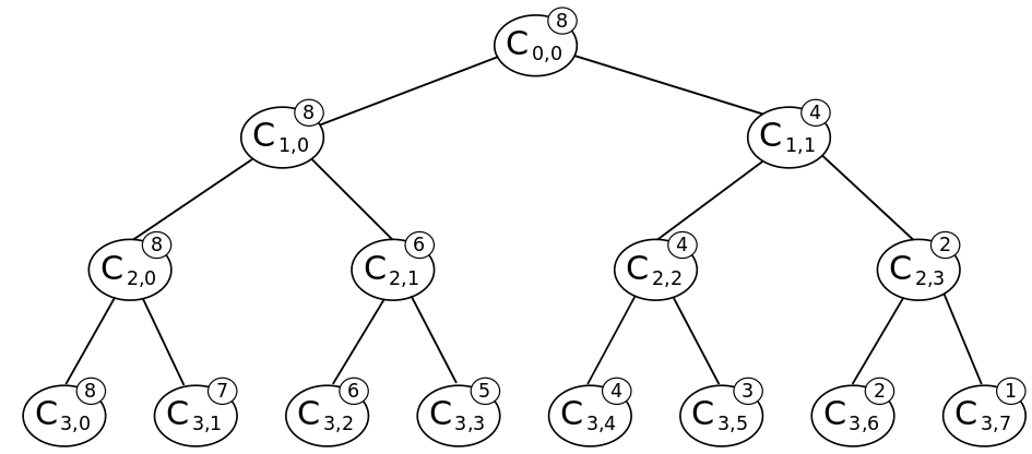
Figure 1: A piecewise constant similarity function described by an oriented binary subtree $\mathcal{T}$. For any pair $(x,x^{\prime})\in\mathcal{X}^{2}$, the similarity score $s_{\mathcal{T}}(x,x^{\prime})$ can be computed very fast in a top-down manner using the heap structure: starting from the initial value $2^{J}$ at the root node, at each internal node $\mathcal{C}_{j,k}$, the score remains unchanged if $(x,x^{\prime})$ moves down to the left sibling and one subtracts $2^{J-(j+1)}$ from it if $(x,x^{\prime})$ moves down to the right.

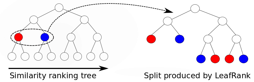
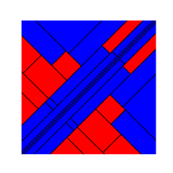
Figure 2: Symmetric split produced by the Symmetric LeafRank procedure.

6.3 Representation of proposal functions for $\mathcal{X}\times\mathcal{X}=\mathbb{R}\times\mathbb{R}$

We illustrate visually the outcomes of TreeRank for different proposition regions, for a similarity function on the unit square $[0,1]\times[0,1]$. To obtain a symmetric similarity function, a natural approach is to transform the data using any function $f:\mathcal{X}\times\mathcal{X}\to\text{Im}(f)$ such that $f(x,x^{\prime})=f(x^{\prime},x)$ and then choose a collection of regions $\mathcal{D}\subset\mathcal{P}(\text{Im}(f))$, to form $\mathcal{C}$ such that

$$\mathcal{C}=\left\{x,x^{\prime}\in\mathcal{X}\times\mathcal{X}\;|\;f(x,x^{\prime})\in D\right\}_{D\in\mathcal{D}}.$$

The $i$-th element of the vector $f(x,x^{\prime})$ will be written $f^{(i)}(x,x^{\prime})$.

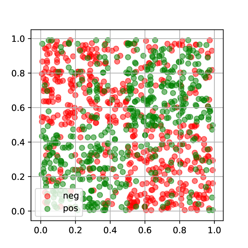
(a) Training pairs

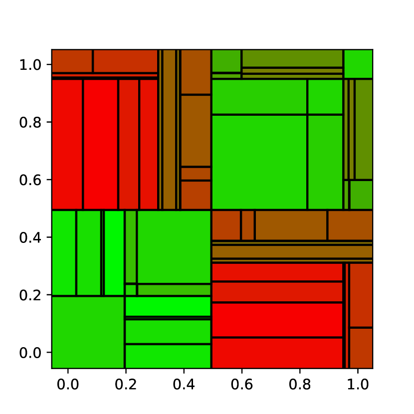
(b) $C_{\text{sq}}$

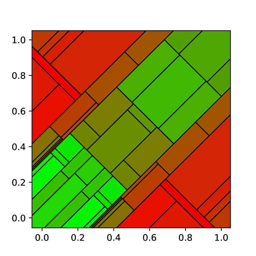
(c) $C_{\text{diag}}$

Figure 3: Representation of TreeRank score function with different proposal regions. The $x$-axis corresponds to $x_{1}$ while the $y$-axis corresponds to $x_{1}^{\prime}$.

In that context, we present two approaches:

• Set $f(x,x^{\prime})=\binom{x\vee x^{\prime}}{x\wedge x^{\prime}}$ where $x\vee x^{\prime}$ and $x\wedge x^{\prime}$ respectively stand for the element-wise maximum and minimum of $x$ and $x^{\prime}$. We introduce the collection $\mathcal{C}_{\text{sq}}$ of all regions:

  $$\left\{x,x^{\prime}\in\mathcal{X}\times\mathcal{X}\Big{/}\left(\sigma f^{(i)}(x,x^{\prime})\geq\sigma A\right)\otimes\left(\sigma f^{(i+D)}(x,x^{\prime})\leq\sigma A\right)\right\}$$

  where $i\in\{1,\dots,D\}$, $\sigma\in\{-1,+1\}$, $A\in\mathbb{R}$ and $\otimes$ is the standard XOR.

• Set $f(x,x^{\prime})=\binom{\lvert x-x^{\prime}\rvert}{x+x^{\prime}}$. We introduce the collection $\mathcal{C}_{diag}$ of all regions:

  $$\left\{x,x^{\prime}\in\mathcal{X}\times\mathcal{X}\Big{/}\sigma f^{(i)}(x,x^{\prime})\geq\sigma A\right\}$$

  where $i\in\{1,\dots,D\}$, $\sigma\in\{-1,+1\}$, $A\in\mathbb{R}$.

We illustrate with fig. 3 the results of the outcome of the TreeRank algorithm with either one of these two approaches, in a simple case where $\mathcal{X}=[0,1]$, $\mu(x)=1$, $K=2$ and $\mathbb{P}\{Y=2|X=x\}=0.6\cdot\mathbb{I}\{x\geq 0.5\}+0.2$. More complicated decision regions can be chosen, such as any linear decision function on the transformation $f(x,x^{\prime})$ of the pair $x,x^{\prime}$. As stated in section 3.1, those could be learned for example by an asymmetrically weighted SVM.

6.4 Details about the synthetic data experiments of section 4

Assume a fully grown tree $\mathcal{T}$ of depth $D_{\text{gt}}$, with terminal cells $\mathcal{C}_{l}\subset\mathcal{X}\times\mathcal{X}$ for all $0\leq l\leq L:=2^{D_{\text{gt}}}-1$. The tree is constructed with splits on the transformation of the input space $\mathcal{X}\times\mathcal{X}$ by the function $f$ introduced in lemma 1. The split is chosen by selecting the split variable uniformly at random, and the split value using a uniform law over that variable on the current cell. The distribution of the data is assumed to be defined by $p_{+}$, $F_{+}=\sum_{l=1}^{L}\delta_{l}^{+}\cdot\mathcal{U}(\mathcal{C}_{l})$ and $F_{-}=\sum_{l=1}^{L}\delta_{l}^{-}\cdot\mathcal{U}(\mathcal{C}_{l})$ where $\mathcal{U}(\mathcal{C}_{l})$ is the uniform distribution over $\mathcal{C}_{l}$. Introduce $\sigma$ as the permutation that orders the cells $C_{l}$ by decreasing $\delta_{l}^{+}/\delta_{l}^{-}$, i.e. $\delta_{\sigma(l)}^{+}/\delta_{\sigma(l)}^{-}\geq\delta_{\sigma(l+1)}^{+}/\delta_{\sigma(l+1)}^{-}$ for all $0\leq l\leq L-1$, then the optimal ROC curve ${\rm ROC}^{*}$ is the line that connects the dots $(0,0)$ and $(\sum_{j=0}^{l}\delta_{\sigma(j)}^{-},\sum_{j=0}^{l}\delta_{\sigma(j)}^{+})$ for all $0\leq l\leq L$.

Now we detail our choice for the specification of the parameters $\delta^{+}_{l}$ and $\delta^{-}_{l}$. Assume $\sigma$ to be the identity permutation. To study the ability of our method to retrieve the optimal ROC curve for different levels of statistical noise, introduce a noise parameter $0<\delta<1$ and fix $\delta_{l}^{+}=c_{\delta}^{+}\cdot\delta^{l/L}$, and $\delta_{l}^{-}=c_{\delta}^{-}\cdot\delta^{-l/L}$ for all $0\leq l\leq L$, with $c_{\delta}^{+}$ and $c_{\delta}^{-}$ normalization constants in $l$ such that both sets $\{\delta_{l}^{+}\}_{0\leq l\leq L}$ and $\{\delta_{l}^{-}\}_{0\leq l\leq L}$ sum to one.

When $\delta$ is close to $0$, ${\rm ROC}^{*}$ approaches the unit step, whereas when $\delta$ is close to $1$, ${\rm ROC}^{*}$ approaches the ROC of random assignment. The experiments presented here used $\delta=0.01$, which makes for an ${\rm AUC}^{*}$ of $0.96$ approximately. By varying the parameter $\delta$, one can study the outcome of our approach for different levels of statistical noise.

The first experiment shows that the learned model $s_{D}$ generalizes poorly when positive instances are rare, as shown in the bounds of [21]. The second one that when $D_{n}\sim\sqrt{\log n}$, learned models stay decent, as show by theorem 1. The last experiment illustrates the fact that using an overly deep tree comparatively to the ground truth does not hinder performance, thanks to the global nature of the ranking problem.

6.5 Real data experiments

We compare the performance of our approach to the widely acclaimed metric learning technique LMNN, see [22], as well as a similarity derived from the cosine similarity of a low-dimensional neural network encoding of the instances, optimized for classification with a softmax cross-entropy loss. For that matter, we use the MNIST database with reduced dimensionality by PCA. The neural network approach is inspired by state of the art techniques in applications of similarity learning, such as in facial recognition. It has shown outstanding performance, but is not directly derived from the ranking problem that these systems usually tackle.

The MNIST database of handwritten digits has a training set of 60,000 images and a test set of 10,000 images and is widely used to benchmark classification algorithms. Each image represents a number between 0 and 9 with a monochrome image of $28\times 28$ pixels, which makes for $K=10$ classes and an initial dimensionality of $784$. The standard principal components analysis (PCA) was set to keep $95\%$ of the explained variance, which reduces the dimensionality of the data to $d=153$. This first step was necessary to limit the memory requirements of the LMNN algorithm. We used the implementation of LMNN provided by the python package metric-learn, and changed the regularization parameter to be $0.01$.

The neural network approach learned an encoding $e:\mathcal{X}=\mathbb{R}^{d}\to\mathbb{R}^{d_{e}}$ of size $d_{e}=128$, used for classification at training time, with a simple softmax-cross entropy behind a fully connected $d_{e}\times K$ layer. The encoding was composed of three stacked fully connected layers followed by ReLU activations of sizes $153\times 146$, $146\times 140$ and $140\times 134$, and finally a $134\times 128$ fully connected layer without an activation function. These layer sizes are arbitrary and were simply chosen as a linear interpolation between the input size $d$ and output size $d_{e}$. The similarity between two instances is computed using a simple cosine similarity between their embeddings.

Our approach was based off a ranking forest with for symmetric LeafRank an asymmetric classification tree over the transformed data of fixed depth $5$, see fig. 2 for an exemple of this type of proposal region. The ranking forest aggregates the results of 44 trees of depth 15 learned on only $10^{5}$ pairs each. Refer to [7] and [6] for details on ranking forests. ROC curve plots are shown in fig. 4. For now, our method shows higher performance than the linear metric learning approach, but performs worse than the neural network encoding approach. Further work will aim to improve the performance of our approach, perhaps with a better LeafRank algorithm.

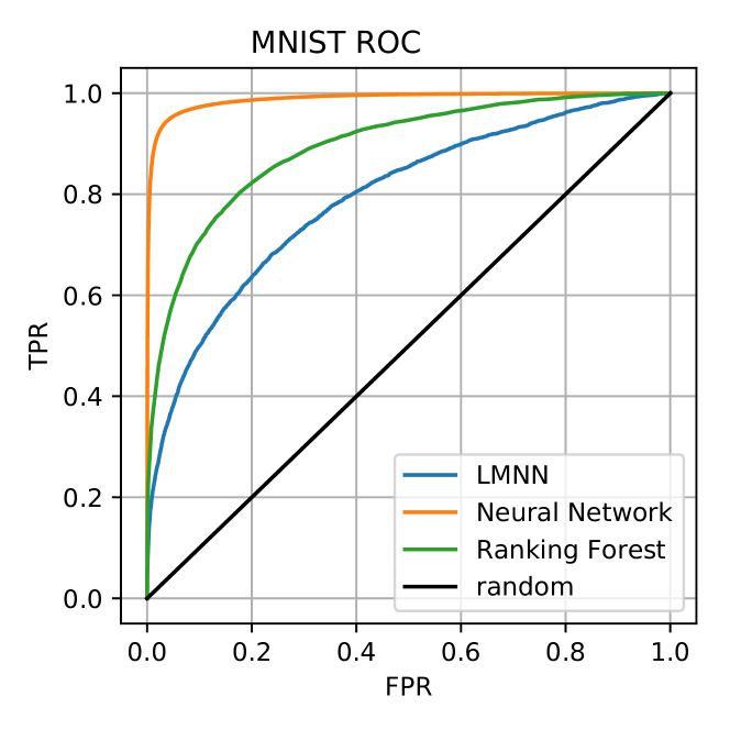
Figure 4: ROC curves for the real data experiments.

References

- [1] A. Bellet and A. Habrard. Robustness and Generalization for Metric Learning. Neurocomputing, 151(1):259–267, 2015.
- [2] A. Bellet, A. Habrard, and M. Sebban. Metric Learning. Morgan & Claypool Publishers, 2015.
- [3] O. Bousquet, S. Boucheron, and G. Lugosi. Introduction to statistical learning theory. In Advanced Lectures on Machine Learning, pages 169–207. 2004.
- [4] L. Breiman, J. Friedman, R. Olshen, and C. Stone. Classification and Regression Trees. Wadsworth and Brooks, 1984.
- [5] Q. Cao, Z.-C. Guo, and Y. Ying. Generalization Bounds for Metric and Similarity Learning. Machine Learning, 102(1):115–132, 2016.
- [6] G. Clémençon, M. Depecker, and N. Vayatis. Ranking Forests. J. Mach. Learn. Res., 14:39–73, 2013.
- [7] S. Clémençon, M. Depecker, and N. Vayatis. Adaptive partitioning schemes for bipartite ranking.
- [8] S. Clémençon and N. Vayatis. Tree-based ranking methods. IEEE Transactions on Information Theory, 55(9):4316–4336, 2009.
- [9] S. Clémençon, G. Lugosi, and N. Vayatis. Ranking and Empirical Minimization of U-Statistics. The Annals of Statistics, 36(2):844–874, 2008.
- [10] T. Fawcett. An Introduction to ROC Analysis. Letters in Pattern Recognition, 27(8):861–874, 2006.
- [11] J. Huo, Y. Gao, Y. Shi, and H. Yin. Cross-modal metric learning for auc optimization. IEEE Transactions on Neural Networks and Learning Systems, PP(99):1–13, 2018.
- [12] A. Jain, L. Hong, and S. Pankanti. Biometric identification. Communications of the ACM, 43(2):90–98, 2000.
- [13] A. K. Jain, A. Ross, and S. Prabhakar. An introduction to biometric recognition. IEEE Transactions on Circuits and Systems for Video Technology, 14(1):4–20, 2004.
- [14] L. Jain, B. Mason, and R. Nowak. Learning Low-Dimensional Metrics. In NIPS, 2017.
- [15] R. Jin, S. Wang, and Y. Zhou. Regularized Distance Metric Learning: Theory and Algorithm. In NIPS, 2009.
- [16] B. Kulis. Metric Learning: A Survey. Foundations and Trends in Machine Learning, 5(4):287–364, 2012.
- [17] A. J. Lee. -statistics: Theory and practice. Marcel Dekker, Inc., New York, 1990.
- [18] B. McFee and G. R. G. Lanckriet. Metric Learning to Rank. In ICML, 2010.
- [19] J. Quinlan. Induction of Decision Trees. Machine Learning, 1(1):1–81, 1986.
- [20] N. Verma and K. Branson. Sample complexity of learning mahalanobis distance metrics. In NIPS, 2015.
- [21] R. Vogel, S. Clémençon, and A. Bellet. A Probabilistic Theory of Supervised Similarity Learning: Pairwise Bipartite Ranking and Pointwise ROC Curve Optimization. In ICML, 2018.
- [22] K. Q. Weinberger and L. K. Saul. Distance Metric Learning for Large Margin Nearest Neighbor Classification. Journal of Machine Learning Research, 10:207–244, 2009.