Quantum coherence and the localization transition

Abstract

A dynamical signature of localization in quantum systems is the absence of transport which is governed by the amount of coherence that configuration space states possess with respect to the Hamiltonian eigenbasis. To make this observation precise, we study the localization transition via quantum coherence measures arising from the resource theory of coherence. We show that the escape probability, which is known to show distinct behavior in the ergodic and localized phases, arises naturally as the average of a coherence measure. Moreover, using the theory of majorization, we argue that broad families of coherence measures can detect the uniformity of the transition matrix (between the Hamiltonian and configuration bases) and hence act as probes to localization. We provide supporting numerical evidence for Anderson and Many-Body Localization (MBL).

For infinitesimal perturbations of the Hamiltonian, the differential coherence defines an associated Riemannian metric. We show that the latter is exactly given by the dynamical conductivity, a quantity of experimental relevance which is known to have a distinctively different behavior in the ergodic and in the many-body localized phases. Our results suggest that the quantum information-theoretic notion of coherence and its associated geometrical structures can provide useful insights into the elusive nature of the ergodic-MBL transition.

I Introduction

One of the conceptual pillars of quantum theory is the superposition principle and, directly arising from it, the notion of quantum coherence Bohm (1989). A quantum state is deemed to be coherent with respect to a complete set of states if it can be expressed as a nontrivial linear superposition of these states. Recently, there has been an effort to formulate a resource theory of quantum coherence Åberg (2006); Baumgratz et al. (2014); Streltsov et al. (2017). The focus of this theory has been quantum information processing tasks, since generating and preserving quantum coherence constitutes one of the essential prerequisites.

In this work, we utilize the powerful tools that arose from this information-theoretic perspective on coherence to study phase transitions in quantum one- and many-body systems. More specifically, we focus on Anderson Anderson (1958a); Lagendijk et al. (2009) and Many-Body Localization (MBL) transitions Basko et al. (2006); Pal and Huse (2010); Nandkishore and Huse (2015). These “infinite temperature” or “eigenstate” phase transitions are characterized by a abrupt change occurring at the level of whole Hamiltonian eigenstates as opposed, e.g., to the ground-state only.

A connection between quantum coherence and the transition of a quantum system from an ergodic phase to a localized one can be conceptually formalized as follows. One of the signatures of localization is the absence of transport, with respect to some properly defined positional degree of freedom. On the other hand, transport properties are governed by the coherence between the Hamiltonian eigenbasis and the positional one. Hence one should expect an abrupt change in the coherence properties of the Hamiltonian eigenvectors at the transition point.

Here we make the above intuition quantitatively precise by investigating the amount of coherence that can be generated on average by the quantum dynamics starting from incoherent states, the Coherence-Generating Power (CGP) of a quantum evolution. Such quantities essentially capture the difference between two complete orthonormal sets of eigenstates associated with two hermitian operators Zanardi and Campos Venuti (2018a); Styliaris and Zanardi (2019). We first show that a well-studied quantity in localization, the escape probability (or, equivalently, the second participation ratio) can be expressed directly as a coherence average. We then argue that broad families of coherence measures, arising from the the resource-theoretic perspective, can be used to define an “order parameter” for localization. We provide supporting numerical evidence for both Anderson and MBL transitions. Moreover, we show that the differential-geometric version of our average coherence is exactly given by an infinite temperature dynamical conductivity, an experimentally accessible quantity, which is known to behave differently in the ergodic and MBL phases Prelovšek et al. (2017). These findings open the possibility of observing experimentally the coherence generating power of quantum dynamics.

This paper is organized as follows. In section II we introduce measures of coherence for quantum states and explain how one can average coherence over a complete set of states in order to obtain the associated CGP, i.e., a quantifier of coherence for unitary quantum operations. We then investigate general mathematical properties of the aforementioned coherence averages and connect with the theory of matrix majorization and the escape probability. In section III we examine, both analytically and numerically, the behavior of two of the introduced measures in the Anderson localization transition and connect with the associated localization length. In section IV we numerically study the introduced measures for a many-body system that exhibits a transition to a MBL phase. In section V we turn to the Riemannian metric that results from the average coherence between bases that differ infinitesimally and relate with the MBL transition. Finally, in section VI we conclude with a discussion and future work. All proofs can be found in section A of the Appendix.

II Quantum coherence of states and operations

II.1 Coherence of states

Consider a quantum system, described by a finite dimensional Hilbert space $\mathcal{H}\cong\mathbb{C}^{d}$. A state $\ket{\psi}\in\mathcal{H}$ is deemed coherent with respect to a fiducial orthonormal basis $\left\{\ket{\phi_{i}}\right\}_{i=1}^{d}$ if the expansion $\ket{\psi}=\sum_{i}a_{i}\ket{\phi_{i}}$ contains more than one non-vanishing term, otherwise it is called incoherent. This notion extends straightforwardly to the set of density operators $\mathcal{S}(\mathcal{H})$. Any $\rho\in\mathcal{S}(\mathcal{H})$ is regarded as coherent with respect to the preferred basis if the corresponding matrix $\rho_{ij}$ has nonzero off-diagonal elements, otherwise it is termed incoherent.

Quantum coherence is usually defined relative to a reference basis. In fact, one needs a weaker notion than that of a basis, since phase degrees of freedom and ordering of an orthonormal basis $\left\{\ket{\phi_{i}}\right\}_{i=1}^{d}$ are physically redundant. In other terms, bases differing by transformations of the form $\ket{\phi_{j}}\mapsto e^{i\theta_{j}}\ket{\phi_{\pi(j)}}$ ($\pi\in S_{d}$ is a permutation) are equivalent as far as coherence is concerned. The relevant object, taking into account this freedom, is a complete set of orthogonal, rank-1 projection operators $B=\left\{\Pi_{i}\right\}_{i=1}^{d}$, where $\Pi_{i}\coloneqq\ket{\phi_{i}}\!\bra{\phi_{i}}$. In the rest of this work, we will refer for convenience to the set $B$ itself as a “basis”.

While all states non-diagonal in $B$ carry coherence, some of them might resemble incoherent states more than others. This notion is made precise by the introduction of ($B$-dependent) functionals, $c_{B}:\mathcal{S}(\mathcal{H})\to\mathbb{R}_{0}^{+}$ that are said to quantify coherence Baumgratz et al. (2014). Quantifiers of coherence (also called coherence monotones) satisfy $c_{B}(\rho_{\operatorname{inc}})=0$ for all states diagonal in $B$ and, in addition, are non-increasing under the free operations of the resource theory . In this work, we make use of the 2-coherence and the relative entropy of coherence, defined respectively by

$$c^{(2)}_{B}(\rho) \coloneqq\left\|\left(\mathcal{I}-\mathcal{D}_{B}\right)\rho\right\|^{2}_{2}=\sum_{i\neq j}\left|\rho_{ij}\right|^{2}$$ (1a)

$$c^{(\operatorname{rel})}_{B}(\rho) \coloneqq S\left[\mathcal{D}_{B}\left(\rho\right)\right]-S\left(\rho\right)\,\;,$$ (1b)

where we have introduced the $B$-dephasing superoperator

$$\mathcal{D}_{B}(X)\coloneqq\sum_{i=1}^{d}\Pi_{i}X\Pi_{i}\,\;,$$ (2)

$S$ above denotes the usual von-Neumann entropy $S(\rho)\coloneqq-\operatorname*{Tr}\left(\rho\log(\rho)\right)$ and the (Schatten) 2-norm of an operator $X$ is defined as $\left\|X\right\|_{2}\coloneqq\sqrt{\operatorname*{Tr}\left(X^{\dagger}X\right)}$. Relative entropy of coherence is a central measure in the resource theories of coherence and admits an operational interpretation, e.g., as a conversion rate of information-theoretic protocols Winter and Yang (2016); Zhao et al. (2018). The 2-coherence admits an interpretation as an escape probability, as will be shown momentarily .

II.2 Coherence of unitary quantum processes via probabilistic averages

In this section we discuss how, given a coherence measure $c_{B}$ and a unitary superoperator $\mathcal{U}$, one can capture the ability of the unitary $\mathcal{U}$ to generate coherence by computing the average amount of coherence that can be generated starting from incoherent states. This is the Coherence-Generating Power (CGP) of the quantum operation $\mathcal{U}$ Zanardi et al. (2017a, b); Styliaris et al. (2018); Zanardi and Campos Venuti (2018a).

Consider a basis $B=\left\{\Pi_{i}\right\}_{i=1}^{d}$ and define a probabilistic ensemble of incoherent states, i.e., a random variable $\rho_{\operatorname{inc}}(\boldsymbol{p})=\sum_{i}p_{i}\Pi_{i}$, where $\left\{p_{i}\right\}_{i}$ $(p_{i}\geq 0$, $\sum_{i}p_{i}=1)$ are random and distributed according to a prescribed measure $\mu(\boldsymbol{p})$. Then, the corresponding CGP

$$C\left(\mathcal{U},c_{B},\mu\right)\coloneqq\int d\mu(\boldsymbol{p})\,c_{B}\left[\mathcal{U}\left(\rho_{\operatorname{inc}}(\boldsymbol{p})\right)\right]$$ (3)

characterizes the average effectiveness of the quantum process $\mathcal{U}$ to generate coherence out of random incoherent states in $B$. Since the unitary $\mathcal{U}(X)=UXU^{\dagger}$ can be thought of as connecting the bases $B$ and $B^{\prime}=\{\mathcal{U}\left(\Pi_{i}\right)\}_{i}$, one can also interpret $C\left(\mathcal{U},c_{B},\mu\right)$ as the average coherence with respect to $B$ of a random state which is incoherent in $B^{\prime}$.

Without any additional structure, it is a natural choice to consider averaging only over pure states with equal weight over each of them , i.e., take

$$\mu_{\operatorname{unif}}(\boldsymbol{p})\coloneqq\frac{1}{d}\sum_{i}\delta\left(\boldsymbol{p}-\boldsymbol{e}_{i}\right)$$ (4)

where $(\boldsymbol{e}_{i})_{j}\coloneqq\delta_{ij}$ . This choice directly leads to the expression

$$C\left(\mathcal{U},c_{B},\mu_{\operatorname{unif}}\right)=\frac{1}{d}\sum_{i=1}^{d}c_{B}\left[\mathcal{U}\left(\Pi_{i}\right)\right]\,\;.$$ (5)

We now simplify Eq. (5) when the coherence measure is the 2-coherence or the relative entropy of coherence, namely for

$$C^{(2)}_{B}\left(\mathcal{U}\right) \coloneqq C\left(\mathcal{U},c^{(2)}_{B},\mu_{\operatorname{unif}}\right)\,\;,$$ (6a)

$$C^{(\operatorname{rel})}_{B}\left(\mathcal{U}\right) \coloneqq C\left(\mathcal{U},c^{(\operatorname{rel})}_{B},\mu_{\operatorname{unif}}\right)\,\;.$$ (6b)

Proposition 1.

Let $B=\left\{\Pi_{i}\right\}_{i=1}^{d}$ be a basis, $\mathcal{U}$ a unitary quantum process and $X_{\mathcal{U}}$ denote the bistochastic matrix with elements $\left(X_{\mathcal{U}}\right)_{ij}\coloneqq\operatorname*{Tr}\left(\Pi_{i}\,\mathcal{U}(\Pi_{j})\right)$. Then,

$$C^{(2)}_{B}\left(\mathcal{U}\right)=1-\frac{1}{d}\operatorname*{Tr}\left(X_{\mathcal{U}}^{T}X_{\mathcal{U}}\right)\,\;.$$ (7)

and

$$C^{(\operatorname{rel})}_{B}\left(\mathcal{U}\right)=H(X_{\mathcal{U}})\,\;,$$ (8)

where $H(X)\coloneqq-\frac{1}{d}\sum_{i,j}X_{ij}\log(X_{ij})$ denotes the generalization of the Shannon entropy over bistochastic matrices.

The two CGP quantities are related as

$$C_{B}^{(\operatorname{rel})}\geq-\log\left(1-C_{B}^{(2)}\right)\,\;.$$ (9)

The inequality follows from the above Proposition, together with the concavity of the logarithmic function.

II.3 General properties of coherence-generating power measures

Both quantities $C_{B}^{(2)}(\mathcal{U})$ and $C_{B}^{(\operatorname{rel})}(\mathcal{U})$ introduced earlier can be considered as functions of the (transition) matrix $X_{\mathcal{U}}$, instead of $\mathcal{U}$ itself. In other words, the phases associated with $U_{ij}$ (treated as a matrix in the $B$ basis) are irrelevant. In fact, as we will show momentarily, this is a general feature of any CGP measure $C\left(\mathcal{U},c_{B},\mu_{\operatorname{unif}}\right)$ arising from a coherence monotone $c_{B}$.

Motivated by the above observation, we define as a generalized CGP measure any function $f_{B}$ mapping bistochastic matrices to non-negative real numbers such that:

1. $f_{B}\left(\Pi\right)=0$ if $\Pi\in S_{d}$ is a permutation.

2. $f_{B}\left(\Pi X\Pi^{\prime}\right)=f_{B}\left(X\right)$, where $\Pi,\Pi^{\prime}\in S_{d}$ are permutations.

3. $f_{B}\left(MX\right)\geq f_{B}\left(X\right)$ for any bistochastic matrix $M$.

Proposition 2.

Let $c_{B}$ be a coherence measure. Then, the corresponding Coherence-Generating Power $f_{B}(X_{\mathcal{U}})\coloneqq C\left(\mathcal{U},c_{B},\mu_{\operatorname{unif}}\right)$ satisfies $\mathrm{(i)-(iii)}$ above.

On physical grounds, all quantities $C\left(\mathcal{U},c_{B},\mu_{\operatorname{unif}}\right)$ are expected to quantify how “uniform” or “spread” is the transition matrix $X_{\mathcal{U}}$ between the bases $B$ and $B^{\prime}=\mathcal{U}(B)$. This intuition is reflected in part (iii) of 2: “post-processing” the transition matrix $X\mapsto MX$ by any bistochastic matrix $M$ will certainly increase any CGP measure $C\left(\mathcal{U},c_{B},\mu_{\operatorname{unif}}\right)$, where $c_{B}$ can be any coherence monotone.

Generalized CGP measures can be thought of as functions that characterize the uniformity of a (bistochastic) matrix. They always achieve their maximum value over the transition matrix $\left(X_{\mathcal{V}}\right)_{ij}=1/d$, i.e., when $\mathcal{V}$ connects two unbiased bases, as follows by combining properties $(ii)$ and $(iii)$. In a similar manner, the minimum value is achieved over permutation matrices and is set to zero (as a normalization) by $(i)$. For instance, any concave function that satisfies properties $(i)$ and $(ii)$ automatically satisfies $(iii)$, i.e., is a generalized CGP measure.

Examples of generalized measures arising from previous works on CGP (see Zanardi et al. (2017b); Zanardi and Campos Venuti (2018b); Styliaris and Zanardi (2019)) are

$$f_{B}^{(\det)}\left(X_{\mathcal{V}}\right) \coloneqq 1-\left|\det\left(X_{\mathcal{V}}\right)\right|^{\frac{1}{d}}$$ (10)

$$f_{B}^{(\infty)}\left(X_{\mathcal{V}}\right) \coloneqq\left\|I-X_{\mathcal{V}}^{T}X_{\mathcal{V}}\right\|_{\infty}\,\;,$$ (11)

where $\left\|\left(\cdot\right)\right\|_{\infty}$ denotes the operator norm. Notice that $f_{B}^{(\det)}(X_{\mathcal{V}})=1-\left(\prod_{i}s_{i}\right)^{\frac{1}{d}}$ and also $0\leq f_{B}^{(\det)}\left(X_{\mathcal{V}}\right)\leq 1$, while $f_{B}^{(\infty)}\left(X_{\mathcal{V}}\right)=1-s_{d}^{2}$ (here $s_{i}$ are the singular values of $X_{\mathcal{V}}$ sorted in decreasing order).

A systematic way to capture the amount of uniformity of a matrix is provided by the notion of multivariate majorization Marshall et al. (2011). An example is column majorization, in which a stochastic matrix $X$ column majorizes another stochastic matrix $Y$, denoted as $X\succ^{c}Y$, if $X^{c}_{i}\succ Y^{c}_{i}$ $\forall i$; here $X^{c}_{i}$ and $Y^{c}_{i}$ stand for the $i^{\text{th}}$ column vector of $X$ and $Y$, respectively, and “$\succ$” denotes ordinary majorization of probability vectors.

It is then natural to ask whether the CGP quantities $C\left(\mathcal{U},c_{B},\mu_{\operatorname{unif}}\right)$ arising from different coherence measures $c_{B}$ jointly capture some notion of uniformity of the transition matrix $X_{\mathcal{U}}$, as described by multivariate majorization. We answer this in the affirmative via the proposition below.

Proposition 3.

Let $c_{B}$ be a coherence measure. Then, the corresponding Coherence-Generating Power $f_{B}(X_{\mathcal{U}})\coloneqq C\left(\mathcal{U},c_{B},\mu_{\operatorname{unif}}\right)$ considered over bistochastic matrices is a monotone of column majorization, i.e., $X\succ^{c}Y$ $\Rightarrow$ $f_{B}(X)\leq f_{B}(Y)$. Conversely, if $f_{B}(X)\leq f_{B}(Y)$ for all $f_{B}$ arising from continuous coherence monotones over pure states, then $X\succ^{c}Y$.

The last part of the above proposition establishes the fact that there are enough coherence monotones over pure states one can consider such that, if all corresponding measures $f_{B}$ are monotonic, then column majorization is guaranteed. In other words, these functions form a complete set of monotones. In that sense, the defined family of CGP measures jointly captures a notion of uniformity for the transition matrix that is at least as strict as column majorization.

II.4 Coherence and escape probability

Let us consider a finite-dimensional quantum system whose dynamics is specified by a Hamiltonian $H$. Suppose the system is initialized in a state $\ket{\psi}$ and one is interested in the escape probability

$$\mathcal{P}_{\psi}\coloneqq 1-\overline{\left|\braket{\psi}{e^{-iHt}}{\psi}\right|^{2}}\,\;,$$ (12)

where the overline denotes the infinite time-average

$$\overline{f(t)}\coloneqq\lim_{T\to\infty}\frac{1}{T}\int_{0}^{T}dt\,f(t)\,\;.$$ (13)

For instance, in the case of a particle hopping on a lattice which is initialized over a single site $j$, $\mathcal{P}_{j}$ corresponds to the average probability of the particle escaping the initial site.

At this point, let us note that in finite dimensions observable quantities such as $\braket{A(t)}\coloneqq\operatorname*{Tr}[A(t)\rho_{0}]=\operatorname*{Tr}[A\rho(t)]$ do not converge to any limit as $t\to\infty$. Instead they start from an initial value and then oscillate around a value given by $\overline{\braket{A(t)}}$ Reimann (2008); Linden et al. (2009); Campos Venuti and Zanardi (2010); Campos Venuti et al. (2011). Since if a function $f(t)$ has a limit for $t\to\infty$, this limit must coincide with $\overline{f(t)}$, the infinite time average provides a way to extract the infinite time limit even when the latter strictly speaking does not exist.

If the Hamiltonian in consideration has non-degenerate energy gaps (also known as the non-resonance condition), the effective dimension $d_{\mathrm{eff}}\coloneqq(1-\mathcal{P}_{\psi})^{-1}$ dictates the equilibration properties of the system: the larger $d_{\mathrm{eff}}$ the smaller are the temporal fluctuations of the observables around their mean values Linden et al. (2009); Reimann (2008), i.e., equilibration is stronger. Since many-body localization is a mechanism by which quantum systems can escape equilibration, it is perhaps no surprise that the effective dimension is related to the localization transition (see the Appendix C for more details on related quantities).

After introducing the basic framework, we are now ready to present our first result. The following Proposition establishes the fact that the 2-coherence of a state, quantified with respect to the Hamiltonian eigenbasis, is the time-averaged escape probability of the state.

Proposition 4.

Let $H=\sum_{i}E_{i}\ket{\phi_{i}}\!\bra{\phi_{i}}$ be a non-degenerate Hamiltonian.

1. For any state $\ket{\psi}$,

   $$\mathcal{P}_{\psi}=c_{B}^{(2)}(\ket{\psi}\!\bra{\psi})\,\;,$$ (14)

   where $B=\left\{\ket{\phi_{i}}\!\bra{\phi_{i}}\right\}_{i}$ is the eigenbasis of the Hamiltonian.

2. Denote the escape probability averaged over a set of orthonormal states $B^{\prime}=\left\{\ket{i}\!\bra{i}\right\}_{i=1}^{d}$ as

   $$\mathcal{P}_{B^{\prime}}\coloneqq\frac{1}{d}\sum_{i=1}^{d}\mathcal{P}_{i}\,\;.$$ (15)

   Then,

   $$\mathcal{P}_{B^{\prime}}=C_{B}^{(2)}(\mathcal{V})=C_{B^{\prime}}^{(2)}(\mathcal{V}^{\dagger})\,\;,$$ (16)

   where $B=\left\{\ket{\phi_{i}}\!\bra{\phi_{i}}\right\}_{i}$ is the eigenbasis of the Hamiltonian and $\mathcal{V}(\cdot)\coloneqq V\left(\cdot\right)V^{\dagger}$, where $V=\sum_{i}\ket{i}\!\bra{\phi_{i}}$ is the intertwiner between $B$ and $B^{\prime}$.

The last equation above demonstrates that the role of the bases $B$ and $B^{\prime}$ can be interchanged. For instance, one can equivalently think in terms of the average coherence over Hamiltonian eigenstates, quantified with respect to the position basis.

A physically relevant family of unitary transformations $\mathcal{U}_{t}$ is the time evolution generated by the Hamiltonian of a system. One can, for instance, consider the time-average of $C_{B^{\prime}}^{(2)}(\mathcal{U}_{t})$. For a Hamiltonian with non-degenerate energy gaps, the aforementioned quantity admits the closed form expression

$$\overline{C_{B^{\prime}}^{(2)}(\mathcal{U}_{t})}=1-\frac{2}{d}\sum_{ij}\braket{X^{c}_{i},X^{c}_{j}}^{2}+\frac{1}{d}\sum_{i}\braket{X^{c}_{i},X^{c}_{i}}^{2}\,\;,$$ (17)

here $X^{c}_{i}$ stands for the column vector of the transition matrix $X_{\mathcal{V}}$, while $V=\sum_{i}\ket{i}\!\bra{\phi_{i}}$ is the intertwiner between the Hamiltonian eigenbasis $B=\{\ket{\phi_{i}}\!\bra{\phi_{i}}\}$ and $B^{\prime}=\{\ket{i}\!\bra{i}\}_{i}$. In fact, the resulting quantity $f_{B}^{(\text{time-avg})}(X_{\mathcal{V}})\coloneqq\overline{C_{B^{\prime}}^{(2)}(\mathcal{U}_{t})}$ fails to be a generalized CGP measure. The details can be found in Appendix B of the Appendix.

The identification between return probability and 2-coherence gives a physical interpretation to the latter and its associated CGP. More importantly, the escape (or return) probability is a well-known measure in the theory of localization Anderson (1958b); Luitz and Lev (2017) and the fact that it can be thought of as coherence gives rise to the question: can other measures arising from the resource theoretic framework of coherence give rise to probes of localization in a similar manner? In what follows, we demonstrate that this is indeed the case, by considering Anderson and MBL.

III Coherence-generating power and localization in the 1-D Anderson model

The Anderson model Anderson (1958b) in one dimension is described by the Hamiltonian

$$H_{W}=-\sum_{i=1}^{L}\left(\ket{i}\!\bra{i+1}+\ket{i+1}\!\bra{i}\right)+\sum_{i=1}^{L}\epsilon_{i}\ket{i}\!\bra{i}$$ (18)

over $L$ sites (i.e., $d=L$) with periodic boundary conditions, where the on-site energies $\epsilon_{i}$ are independent and identically distributed (i.i.d.) random variables and follow a uniform distribution of width $2W$. It is known that the model is localized for any degree of disorder $W>0$ Hundertmark (2008).

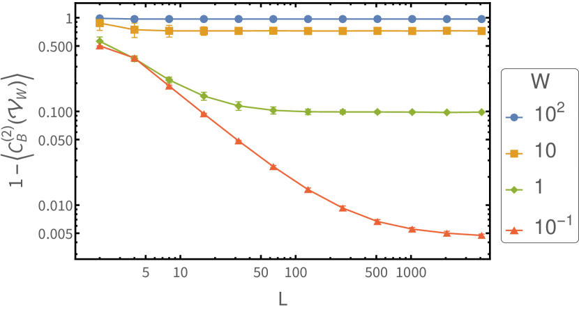
(a) average return probability (Anderson)

(b) relative entropy CGP (Anderson)

Figure 1: (a) Log-log plot of the average return probability $1-\braket{C_{B}^{(2)}\left(\mathcal{V}_{W}\right)}$ as a function of the system size $L$ for different values of the disorder strength $W$. The system is in the localized phase for all $W>0$, since the asymptotic escape probability is strictly less that 1 for $L\to\infty$.
(b) Log-linear plot of $\braket{C_{B}^{(\operatorname{rel})}\left(\mathcal{V}_{W}\right)}$ as a function of the system size $L$ for different values of the disorder strength $W$. The system is in the localized phase for all $W>0$, in which the asymptotic value is finite. In the ergodic phase ($W=0$) $\braket{C_{B}^{(\operatorname{rel})}\left(\mathcal{V}_{W}\right)}$ diverges logarithmically.
The number of realizations range from $30\,000$ for small sizes to just 8 for the largest size. Error bars represent one standard deviation. Entropy has logarithm with base 2.

Localization can be dynamically characterized by the absence of transport, a notion referring to the interplay between the “position” basis $B^{\prime}=\left\{\ket{i}\!\bra{i}\right\}_{i=1}^{L}$ in Eq. (18) and the Hamiltonian eigenbasis $B$. Here, we consider coherence quantified with respect to the latter basis. Let us now examine the behavior of functionals $C_{B}(\mathcal{V}_{W})$, where the unitary $V_{W}$ is the intertwiner between Hamiltonian and position eigenbases. In fact, 4 immediately implies that $\braket{C_{B}^{(2)}(\mathcal{V}_{W})}$ is a probe to localization ($\braket{\cdot}$ denotes averaging over disorder). More specifically, localization implies that in thermodynamic limit the return probability (averaged over disorder) in the localized phase is non-vanishing, i.e., $\lim_{L\to\infty}\braket{\overline{}{\braket{j}{e^{-iH_{W}t}|j}\right|^{2}}{>}{0}}$ for any $W>0$. In turn, this is equivalent to $\mathcal{P}_{j}<1$ (in the thermodynamic limit) for all sites $j$, hence also

$$\lim_{L\to\infty}\braket{C_{B}^{(2)}\left(\mathcal{V}_{W}\right)}<1$$ (19)

by Eq. (15). Notice that $H_{W}$ for $W>0$ is generically non-degenerate so 4 applies. We verify this claim by numerical simulations (see Figure 1).

The Hamiltonian $H_{W=0}$ is degenerate in the ergodic phase, hence the intertwiner $\mathcal{V}_{H_{W=0}}$ is not well-defined. Nevertheless, as we show in Appendix D, for any choice of eigenbasis of $H_{W}$ it holds that

$$\lim_{L\to\infty}C_{B}^{(2)}\left(\mathcal{V}_{W=0}\right)=1\,\;,$$ (20)

hence the average coherence $\braket{C_{B}^{(2)}\left(\mathcal{V}_{W}\right)}$ unambiguously distinguishes the two behaviors.

The role of the quantity $C_{B}^{(2)}(\mathcal{V}_{W})$ might seem special as a probe to localization due to its interpretation as average escape probability. In fact, other measures, arising from an information-theoretic viewpoint of coherence have analogous properties. Let’s now consider the relative entropy CGP of the intertwiner, namely $C^{(\operatorname{rel})}_{B}(\mathcal{V}_{W})$. Its value as a function of the system size $L$ for different values of the disorder strength $W$ is plotted in Figure 1. In the ergodic phase $W=0$ it diverges logarithmically

$$C^{(\operatorname{rel})}_{B}(\mathcal{V}_{W=0})\sim\log(L)\,\;.$$ (21)

This can be easily verified analytically for an intertwiner connecting two mutually unbiased bases, i.e., for $\left|\braket{i}{\phi_{j}}\right|=1/\sqrt{L}$ for all $i,j$. In that case Eq. (21) holds with equality, as it directly follows from 1. In Appendix D we show that the result again holds in the thermodynamic limit independently of the specific choice for the intertwiner.

We now provide a non-rigorous argument to relate the averages $\braket{C^{(2)}_{B}(\mathcal{V}_{W>0})}$ and $\braket{C^{(\operatorname{rel})}_{B}(\mathcal{V}_{W>0})}$ to the corresponding localization lengths $\xi_{j}$. In the localized phase, the eigenvectors typically decay exponentially, i.e.,

$$\left|\braket{i}{\phi_{j}}\right|^{2}\leq c_{j}\exp\left(-|i-\alpha_{j}|/\xi_{j}\right)\,\;,$$ (22)

where $\alpha_{j}$ is the site around which $\ket{\phi_{j}}$ is localized, while due to the periodic boundary conditions $\left|i-\alpha_{j}\right|$ above should be understood as $\min(\left|i-\alpha_{j}\right|,\left|i-\alpha_{j}\pm L\right|)$). If one uses the ansatz

$$\left(X_{\mathcal{V}_{W}}\right)_{ji}=\left|\braket{i}{\phi_{j}}\right|^{2}=c_{j}\exp\left(-|i-\alpha_{j}|/\xi_{j}\right)\,\;,$$ (23)

then for $L\gg 1$

$$\braket{C^{(2)}_{B}(\mathcal{V}_{W>0})}\cong 1-\frac{1}{L}\sum_{j}\frac{\tanh^{2}[(2\xi_{j})^{-1}]}{\tanh(\xi^{-1}_{j})}$$ (24a)

and

$$\braket{C^{(\operatorname{rel})}_{B}(\mathcal{V}_{W>0})}\cong\\ \frac{1}{L}\sum_{j=1}^{L}\left(\left[\xi_{j}\sinh(1/\xi_{j})\right]^{-1}-\ln\left(\tanh\left[(2\xi_{j})^{-1}\right]\right)\right)$$ (24b)

(entropy here has natural logarithm). A detailed derivation can be found in Appendix E.

The expression (24b) for $\xi_{j}\gg 1$ can be expanded as $\braket{C_{B}^{(\operatorname{rel})}\left(\mathcal{V}_{\Gamma}\right)}=\frac{1}{L}\sum_{j=1}^{L}\left(1+\ln\left(2\xi_{j}\right)+O(\xi_{j}^{-2})\right)$, which is consistent with the numerically observed behavior that it remains finite in the localized phase while it diverges logarithmically as a function of $L$ in the ergodic one.

The accuracy of equations (24) can be assessed by comparing with cases for which an analytical expression can be obtained for the localization lengths $\xi_{j}$ as a function of the disorder strength. We now consider such a case, described by a Hamiltonian as in Eq. (18), but with on-site energies that follow a Cauchy distribution with parameter $\Gamma$ and vanishing mean (also known as Lloyd model Lloyd (1969)). We focus for concreteness on Eq. (24a) and we denote the corresponding Hamiltonian and intertwiner as $H_{\Gamma}$ and $\mathcal{V}_{\Gamma}$, respectively. Utilizing a well-known result from Thouless Thouless (1972) that connects the localization length with the energy spectrum, one can express the RHS of Eq. (24a) as a function of the disorder strength $\Gamma$. This allows for a direct comparison with numerical evaluations of the mean $\braket{C_{B}^{(2)}(\mathcal{V}_{\Gamma})}$, yielding a sound agreement for small disorder ($\Gamma<1$). We present the details in Appendix F of the Appendix.

IV Coherence-generating power and many-body localization

We now turn to a disordered quantum many-body system admitting a phase diagram with an ergodic phase at low enough disorder and an MBL phase at strong disorder. For this purpose, we consider a transverse-field Heisenberg spin-1/2 chain in a random magnetic field (along the $\hat{z}$-axis) over $L$ sites ($d=2^{L}$) with periodic boundary conditions, described by the Hamiltonian

$$H_{\mathrm{XXX}} =\frac{1}{2}\sum_{i=1}^{L}\left[\sigma_{i}^{x}\sigma_{i+1}^{x}+\sigma_{i}^{y}\sigma_{i+1}^{y}+\sigma_{i}^{z}\sigma_{i+1}^{z}\right]$$

$$+h_{x}\sum_{i=1}^{L}\sigma_{i}^{x}+\sum_{i=1}^{L}w_{i}\sigma_{i}^{z}\,\;,$$ (25)

where the $h_{x}$ is the strength of the transverse field and the local field strengths are i.i.d. random variables with uniform distribution $w_{i}\in\left[-W,W\right]$. Notice that the transverse field breaks the rotational symmetry of the Hamiltonian. The model has been extensively studied numerically and is known to exhibit a transition from an ergodic to an MBL phase at disorder strength $W_{C}\approx 3.7$ (in the absence of the transverse field term), see Luitz and Lev (2017); Abanin et al. (2019) and references therein.

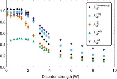
Figure 2: Asymptotic behavior for the slope of the quantities: $\log_{2}\left(1-\braket{C_{B}^{(2)}\left(\mathcal{V}_{W}\right)}\right)=\log_{2}\left(P_{\text{return}}\right)$, $\braket{C_{B}^{(\text{rel})}\left(\mathcal{V}_{W}\right)}$, $\log_{2}\left(1-\braket{f_{B}^{(\det)}\left(X_{\mathcal{V}_{W}}\right)}\right)$, $\log_{2}\left(1-\braket{f_{B}^{(\text{time-avg})}\left(X_{\mathcal{V}_{W}}\right)}\right)$, and $\log_{2}\left(1-\braket{f_{B}^{(\infty)}\left(X_{\mathcal{V}_{W}}\right)}\right)$ for large $L$ as a function of the disorder strength $W$ for the Hamiltonian $H_{\mathrm{XXX}}$ at $h_{x}=0.3$. The slope was extracted for sizes $L=4,6,\cdots,14$, with sample sizes $$20\,000$,$20\,000$,$20\,000$,$8000$,$2000$,$800$$; except at the $W=3.7$, where the sample sizes were doubled. The error bars represent the standard error of the linear fit (see the Appendix H for more details). Entropy has logarithm with base 2.

Similar to the Anderson Hamiltonian, we first study the behavior of the CGP $\braket{C_{B}^{(2)}\left(\mathcal{V}_{W}\right)}$ and $\braket{C_{B}^{(\operatorname{rel})}\left(\mathcal{V}_{W}\right)}$, where $\mathcal{V}_{W}$ is the intertwiner between the Hamiltonian and the configuration space basis, which here is taken to be the product $\bigotimes_{i}\sigma_{i}^{z}$ eigenbasis. We find a distinct behavior of the quantities $\braket{C_{B}^{(2)}\left(\mathcal{V}_{W}\right)}$ and $\braket{C_{B}^{(\operatorname{rel})}\left(\mathcal{V}_{W}\right)}$ between the ergodic and MBL phases of the model, as also hinted from the numerical results in Serbyn et al. (2013); Luca and Scardicchio (2013); Goold et al. (2015); Torres-Herrera and Santos (2015, 2017); Serbyn and Abanin (2017).

For sizes up to $L=14$, none of the studied CGP quantities seems to reach a constant asymptotic value as in the Anderson case. Nonetheless, the (average) return probability $P_{\text{return}}$ as a function of the number of spins $L$ is consistent with an exponential decay

$$P_{\text{return}}\propto 2^{-\lambda^{(2)}_{W}L}=d^{-\lambda^{(2)}_{W}}\,\;.$$ (26)

The extrapolated rates $\lambda^{(2)}_{W}$, plotted in Figure 2, are close to 1 in the ergodic phase, while they drop at the transition point, obtaining a significantly reduced value at the MBL phase. On the other hand, the relative entropy CGP is consistent with a scaling

$$\braket{C_{B}^{(\operatorname{rel})}\left(\mathcal{V}_{W}\right)}=\lambda^{(\operatorname{rel})}_{W}L+\text{const}\,\;,$$ (27)

with a rate $\lambda^{(\operatorname{rel})}_{W}$ that is close to 1 for small disorder and drops significantly in the MBL phase.

We now turn to the generalized CGP measures $f_{B}^{(\det)}$ and $f_{B}^{(\infty)}$, whose behavior is also consistent with a scaling

$$1-\braket{f_{B}^{(x)}\left(X_{\mathcal{V}_{W}}\right)}\propto 2^{-\lambda^{(x)}_{W}L}=d^{-\lambda^{(x)}_{W}}\,\;,$$ (28)

and a rate $\lambda_{W}^{(x)}$ showing distinct behavior in the different phases ($x=\det$ or $x=\infty$). In Appendix G of the Appendix we show that

$$\lambda_{W}^{(\det)}\geq\frac{1}{2}\lambda_{W}^{(2)}\,\;,$$ (29)

which is saturated for small disorder values and is verified by the observed numerical simulations. Exponential decay is also encountered for the time-average $\braket{f_{B}^{(\text{time-avg})}\left(X_{\mathcal{V}_{W}}\right)}$, also plotted in Figure 2. Notice that, although the latter fails to be a generalized CGP measure, it can still be employed to detect the transition. For more details about the numerical simulations see the Appendix H.

For what regards $\braket{C_{B}^{(2)}\left(\mathcal{V}_{W}\right)}$, we can obtain its behaviour in the limit of infinite disorder and in the ergodic phase. First, we write the return probability $P_{\text{return}}\coloneqq 1-\mathcal{P}_{B^{\prime}}=1-\braket{C_{B}^{(2)}\left(\mathcal{V}_{W}\right)}$ as

$$P_{\text{return}}=\frac{1}{d}\sum_{i=1}^{d}\langle i|\mathcal{E}(|i\rangle\langle i|)|i\rangle\,\;,$$ (30)

where $\mathcal{E}\coloneqq\langle\overline{{\cal U}_{t}}\rangle$ is the average of the quantum (superoperator) evolution $\mathcal{U}_{t}(\cdot)=e^{-itH_{\mathrm{XXX}}}(\cdot)e^{itH_{\mathrm{XXX}}}$ and $|i\rangle$ denotes the product $\bigotimes_{i}\sigma_{i}^{z}$ (Ising) basis.

In the limit of strong disorder $\mathcal{E}(|i\rangle\langle i|)=|i\rangle\langle i|$ so that $P_{\text{return}}=1$. Instead, in the ergodic phase, or more precisely assuming that the operators $|i\rangle\langle i|$ are shell-ergodic (see Campos Venuti and Liu (2019)) one obtains $\mathcal{E}(|i\rangle\langle i|)=\rho_{eq}$ where $\rho_{eq}$ is the (microcanonical) equilibrium state (see Campos Venuti and Liu (2019) for more details). This implies that $P_{\text{return}}=(1/d)\mathrm{Tr}(\rho_{eq})=1/d$ thus converging to zero in the thermodynamic limit. One reaches the same conclusion ($P_{\text{return}}\to 0$ albeit possibly with a different speed) if shell ergodicity holds not for all but for sufficiently many basis projectors $|i\rangle\langle i|$.

Finally, we comment on our findings from the typicality point of view. In Zanardi et al. (2017a) it was shown that, if the intertwiner is chosen at random from the unitary group $V\in U(d)$ according to the Haar measure, then $C^{(2)}_{B}$ is concentrated near its mean

$$\braket{C^{(2)}_{B}(\mathcal{V})}_{\text{Haar}}=1-\frac{2}{d+1}$$ (31)

($\braket{\cdot}_{\text{Haar}}$ denotes the Haar average over the intertwiner), with overwhelming probability for large Hilbert space dimension $d$ (here $B$ can be any fixed basis). In other words, the typical rate for $P_{\text{return}}$ is $\lambda^{(2)}_{\text{Haar}}\approx 1$. From that perspective, an ergodic behavior is the typical one, while the MBL case can be seen as a highly atypical outlier.

V Differential geometry of coherence-generating power and MBL

In this section we study the behavior of the CGP $C^{(2)}_{B}(\delta\mathcal{V})$ when the intertwiner $\delta\mathcal{V}$ connects two bases that are “infinitesimally close” to each other. This results in a differential-geometric construction whose central quantity is a Riemannian metric. As we will show, the resulting metric (i) is directly connected to the dynamical conductivity, which is a quantity of experimental relevance, and (ii) behaves distinctly in the MBL and ergodic phases. The detailed mathematical structure is presented in Appendix I.

Consider a complete orthonormal family of states $\left\{\ket{\phi_{i}(\lambda)}\right\}_{i=1}^{d}$, parametrized by a set of parameters $\lambda$. This is the relevant case, for instance, when one studies the eigenvectors associated with a family of Hamiltonians $H(\lambda)$. The infinitesimal adiabatic intertwiner $\delta{\mathcal{V}}$ is a unitary map defined by

$$\delta{\mathcal{V}}\left(\ket{\phi_{i}(\lambda)}\!\bra{\phi_{i}(\lambda)}\right)=\ket{\phi_{i}(\lambda+d\lambda)}\!\bra{\phi_{i}(\lambda+d\lambda)}\,\;,$$ (32)

where $H(\lambda)\ket{\phi_{i}(\lambda)}=E_{i}(\lambda)\ket{\phi_{i}(\lambda)}$.

It can be shown that the CGP of $\delta{\mathcal{V}}$ has the form $C^{(2)}_{B}(\delta{\mathcal{V}})=2gd\lambda^{2}$, where $g$ is a metric given by

$$g \coloneqq\frac{1}{d}\sum_{i=1}^{d}\chi_{i}\,\;,$$ (33a)

$$\chi_{i} \coloneqq\Braket{\frac{\partial\phi_{i}}{\partial\lambda}}{\frac{\partial\phi_{i}}{\partial\lambda}}-\Braket{\phi_{i}}{\frac{\partial\phi_{i}}{\partial\lambda}}\Braket{\frac{\partial\phi_{i}}{\phi_{i}}}{\phi_{i}}\,\;,$$ (33b)

i.e., it is itself a mean of the metrics $\chi_{i}$ which are associated to the vectors $\ket{\phi_{i}}$. When the latter are Hamiltonian eigenstates, $\chi_{i}$ are known as fidelity susceptibilities Zanardi and Paunković (2006); Campos Venuti and Zanardi (2007); You et al. (2007) and the ground state susceptibility $\chi_{0}$ plays a key role in the differential geometric approach to quantum phase transitions Zanardi et al. (2007).

In order to connect with quantities of experimental relevance, let us now consider the thermal analog of the metric $g$. We denote $g_{T}=\sum_{i}p_{i}\chi_{i}$, where $p_{i}=\exp\left(-E_{i}/T\right)/Z$ are the thermal weights and $Z$ denotes the partition function. The quantity $g_{T}$, defined in Kolodrubetz et al. (2017) as a generalization of the fidelity susceptibility at finite temperature ($g=g_{T=\infty}$), can be thought of as the metric associated with the thermal analogue of the CGP $C(\mathcal{V},c_{B}^{(2)},\mu_{T})$, where the measure $\mu_{T}$ weights the Hamiltonian eigenstates with the associated Gibbs weights. The quantity $g_{T}$ can be expressed via the (imaginary part of the) dynamical susceptibility $\chi_{VV}(\omega)$, where $V=\partial_{\lambda}H(\lambda)$. More precisely (see Kolodrubetz et al. (2017)),

$$g_{T}=\int_{0}^{\infty}\frac{d\omega}{\pi}\frac{\chi^{\prime\prime}_{VV}(\omega)}{\omega^{2}}\coth\left(\frac{\omega}{2T}\right).$$ (34)

The above formula is remarkable, as it demonstrates that the, apparently abstract, quantity $C_{B}^{(2)}(\delta\mathcal{V})$ is simply connected with a quantity measurable in experimental setups Helton et al. (2010); Dai (2015); Hauke et al. (2016). We also note that, although Eq. (34) is not straightforwardly applicable in the infinite temperature limit, in this limit one obtains

$$g=g_{T=\infty}=\frac{1}{\pi}\int_{-\infty}^{\infty}\frac{\sigma_{VV}(\omega)}{\omega^{2}}d\omega\,\;,$$ (35)

where $\sigma_{VV}(\omega)$ is the high-temperature dynamical conductivity given by

$$\sigma_{VV}(\omega) =\frac{2\pi}{d}\sum_{n\neq m}\left|V_{n,m}\right|^{2}\delta[\omega-(E_{m}-E_{n})].$$ (36)

In this case, the role of $g$ is played by the d.c. dielectric polarizability Barišić et al. (2016); Prelovšek et al. (2017).

The quantities $g_{T}$ and $g$ not only allow to make contact with experiments, but have also been studied in the context of thermalization and MBL. In particular, it is believed that $g\to\infty$ in the thermodynamic limit, both for the ergodic and the sub-diffusive phase. Instead, in the MBL phase $g\to\mathrm{constant<\infty}$ Prelovšek et al. (2017). In the light of Eq. (33), these results mean that the CGP of the adiabatic intertwiner between nearby Hamiltonians has distinctively different behaviors in the ergodic and in the MBL phases.

VI Conclusions and future works

In this work we have brought together ideas from quantum information and geometry, on the one hand, and the physics of disordered systems on the other. We established a connection between the quantitative approach to coherence, originating from the perspective of quantum resource theories Baumgratz et al. (2014); Streltsov et al. (2017), and localization Anderson (1958b); Basko et al. (2006); Pal and Huse (2010); Nandkishore and Huse (2015).

More specifically, we studied the behavior over the ergodic, Anderson and many-body localized phases in terms of the scaling properties of coherence averages that are associated to the intertwiner connecting the Hamiltonian eigenvectors with the configuration space basis. Furthermore, we built an associated differential-geometric version for infinitesimal perturbations of the Hamiltonian, and showed that the resulting Riemannian metric can be mapped onto known physical quantities which have a sharply distinct behavior in the ergodic and in the MBL phases.

Quantum chaos is often dubbed as the dynamical counterpart of quantum localization and connections between the two have been used to elucidate the physics of chaotic systems Fishman et al. (1982); Haake (2010). Following this correspondence, we conjecture that the CGP can act as a signature of quantum chaos, for example, by identifying the so-called “edge of chaos” Weinstein et al. (2002). Moreover, dynamical quantities like the survival probability Torres-Herrera and Santos (2019) and entangling power Zanardi et al. (2000) (which is the direct analogue of CGP for entanglement) have been applied to the study of chaotic systems like the quantum kicked top Haake (2010), which can be related to measures of CGP, as will be explored in a forthcoming article pre .

Establishing further, more rigorous, theoretical as well as numerical grounds for this connection between the information-theoretic approach to quantum coherence and many-body theory provides a direction for future research.

Appendix A Proofs of Propositions

See 1

Proof.

(i) We follow a procedure similar to the one in Ref. Zanardi et al. (2017a). We make use of the Hilbert-Schmidt inner product $\braket{A,B}\coloneqq\operatorname*{Tr}\left(A^{\dagger}B\right)$ over the space $\mathcal{B}(\mathcal{H})$ of bounded linear operators over $\mathcal{H}$. Starting from Eq. (5) with $c_{B}=c_{B}^{(2)}$, we get

$$C^{(2)}_{B}\left(\mathcal{U}\right) =\frac{1}{d}\sum_{i}\left\|\left(\mathcal{I}-\mathcal{D}_{B}\right)\mathcal{U}\Pi_{i}\right\|_{2}^{2}$$

$$=\frac{1}{d}\sum_{i}\braket{\left(\mathcal{I}-\mathcal{D}_{B}\right)\mathcal{U}\Pi_{i},\left(\mathcal{I}-\mathcal{D}_{B}\right)\mathcal{U}\Pi_{i}}$$

$$=\frac{1}{d}\sum_{i}\left(\left\|\mathcal{U}\Pi_{i}\right\|_{2}^{2}-\left\|\mathcal{D}_{B}\mathcal{U}\Pi_{i}\right\|_{2}^{2}\right)\,\;,$$

where we have used the fact that the dephasing superoperator $\mathcal{D}_{B}\in\mathcal{B}(\mathcal{B}(\mathcal{H}))$ is self-adjoint $\mathcal{D}_{B}^{\dagger}=\mathcal{D}_{B}$ with respect to the Hilbert-Schmidt inner product, as well as a projection $\mathcal{D}_{B}^{2}=\mathcal{D}_{B}$. Unitary invariance of the 2-norm implies $\left\|\mathcal{U}\Pi_{i}\right\|_{2}^{2}=1$. Using the definition Eq. (2), a straightforward calculation gives

$$C^{(2)}_{B}\left(\mathcal{U}\right)=1-\frac{1}{d}\sum_{ij}\left(X_{\mathcal{U}}\right)^{2}_{ji}$$ (37)

which reduces to the claimed result.

(ii) Let us denote the Shannon entropy of a probability vector as $H(\boldsymbol{p})\coloneqq-\sum_{i}p_{i}\log(p_{i})$. Since $S(\mathcal{U}\Pi_{i})=S(\Pi_{i})=0$, Eq. (5) with $c_{B}=c_{B}^{(\operatorname{rel})}$ gives

$$C^{(\operatorname{rel})}_{B}\left(\mathcal{U}\right) =\frac{1}{d}\sum_{i}S(\mathcal{D}_{B}\mathcal{U}\Pi_{i})$$

$$=\frac{1}{d}\sum_{i}S\left(\sum_{j}\left(X_{\mathcal{U}}\right)_{ji}\Pi_{j}\right)$$

$$=\frac{1}{d}\sum_{i}H\left(\left\{\left(X_{\mathcal{U}}\right)_{ji}\right\}_{j}\right)$$

$$=H(X_{\mathcal{U}})\,\;.$$

∎

See 2

Proof.

We first show that, for a fixed coherence measure $c_{B}$, the quantity $C\left(\mathcal{U},c_{B},\mu_{\operatorname{unif}}\right)$ (explicitly given in Eq. (5)) can be expressed as a function of $X_{\mathcal{U}}$. This implies that the phases of $U$ (considered as a matrix in the $B=\{\Pi_{i}\}_{i}=\{\ket{\phi_{i}}\!\bra{\phi_{i}}\}_{i}$ basis, where $\mathcal{U}(X)=UXU^{\dagger}$) are irrelevant.

Consider a pure state $\ket{\psi}$. The value of $c_{B}\left(\ket{\psi}\!\bra{\psi}\right)$ can only depend on the modulus of the coefficients $\left\{\left|\braket{\phi_{i}}{\psi}\right|\right\}_{i=1}^{d}$. This follows from the fact that the unitary transformations $\mathcal{V}(\rho)=V\rho V^{\dagger}$, such that $V\ket{\psi}$ alters the phases or permutes the coefficients $\{\braket{\phi_{i}}{\psi}\}_{i=1}^{d}$, form a subgroup of the Incoherent Operations. Hence all coherence monotones should maintain a constant value over a group orbit. As a result, $c_{B}(\mathcal{U}(\Pi_{j}))$ can be expressed as a function of $\{\left(X_{\mathcal{U}}\right)_{ij}\}_{i=1}^{d}$ (recall $\left(X_{\mathcal{U}}\right)_{ij}=\left|\braket{\phi_{i}}{U}{\phi_{j}}\right|^{2}$). Hence, also $C\left(\mathcal{U},c_{B},\mu_{\operatorname{unif}}\right)$ can be expressed as a function of the whole matrix $X_{\mathcal{U}}$ (in fact, an additive one over the columns).

Property (i) follows directly from the fact that coherence measures vanish over incoherent states. For property (ii), invariance under pre-processing by a permutation $\Pi^{\prime}$ holds since the averaging over the states is uniform. Invariance under post-processing by $\Pi$ holds since unitary transformations that permute the elements of $B$ belong to Incoherent Operators.

We now prove property (iii). First notice that, since the value of $c_{B}\left(\ket{\psi}\!\bra{\psi}\right)$ can only depend on the moduli of the coefficients $\left\{\left|\braket{\phi_{i}}{\psi}\right|\right\}_{i=1}^{d}$, the function $f_{B}(X)$ is in fact well-defined over all bistochastic matrices (and not just unistochastic ones).

Consider a collection of pure states $\{\ket{\psi_{j}}\!\bra{\psi_{j}}\}_{j=1}^{d}$ such that

$$\ket{\psi_{j}}=\sum_{i}\sqrt{(MX_{\mathcal{U}})_{ij}}\ket{\phi_{i}}\,\;.$$ (38)

Then, one has that

$$\operatorname*{Tr}\left(\Pi_{i}\ket{\psi_{j}}\!\bra{\psi_{j}}\right)=\sum_{k}M_{ik}\operatorname*{Tr}\left(\Pi_{k}\,\mathcal{U}(\Pi_{j})\right)\quad\forall i,j\,\;.$$ (39)

To prove the desired inequality of (iii), we will show that $c_{B}\left(\ket{\psi_{j}}\!\bra{\psi_{j}}\right)\geq c_{B}(\mathcal{U}(\Pi_{j}))$ $\forall j$. Indeed, the previous holds true for all coherence measures $c_{B}$ if for every $j$ there exists an Incoherent Operator $\mathcal{E}$ such that $\mathcal{E}\left(\ket{\psi_{j}}\!\bra{\psi_{j}}\right)=\mathcal{U}(\Pi_{j})$. The last is guaranteed (in fact, within Strictly Incoherent Operators) by the main result of Du et al. (2015) which can be applied since, by the bistochasticity of $M$, Eq. (39) implies that $\mathcal{D}_{B}\left(\mathcal{U}(\Pi_{j})\right)\succ\mathcal{D}_{B}\left(\ket{\psi_{j}}\!\bra{\psi_{j}}\right)$.

∎

See 3

Proof.

The first part follows by generalizing the proof of part (iii) of 2. One can directly extend the construction by considering two sets of pure states $\{\ket{\psi_{j}}\!\bra{\psi_{j}}\}_{j=1}^{d}$ and $\{\ket{\psi^{\prime}_{j}}\!\bra{\psi^{\prime}_{j}}\}_{j=1}^{d}$ such that

$$\ket{\psi_{j}} =\sum_{i}\sqrt{Y_{ij}}\ket{\phi_{i}}$$ (40a)

$$\ket{\psi^{\prime}_{j}} =\sum_{i}\sqrt{X_{ij}}\ket{\phi_{i}}\,\;.$$ (40b)

Then the convertibility argument $\ket{\psi_{j}}\!\bra{\psi_{j}}\mapsto\ket{\psi^{\prime}_{j}}\!\bra{\psi^{\prime}_{j}}$ via strictly incoherent operations applies due to the majorization condition, giving the desired result.

For the converse, we will first show that the functions over pure states $c_{B}(\ket{\psi}\!\bra{\psi})=\sum_{i}\phi\left(\operatorname*{Tr}\left(\Pi_{i}\ket{\psi}\!\bra{\psi}\right)\right)$ are monotones, where $\phi$ is any continuous concave function. Indeed, from the main result of Du et al. (2015), a conversion $\ket{\psi}\!\bra{\psi}\mapsto\ket{\psi^{\prime}}\!\bra{\psi^{\prime}}$ via Strictly Incoherent Operations is possible if and only if $\mathcal{D}_{B}(\ket{\psi^{\prime}}\!\bra{\psi^{\prime}})\succ\mathcal{D}_{B}(\ket{\psi}\!\bra{\psi})$ . However, a standard result by Hardy, Littlewood and Pólya states that for two probability vectors it holds that $\boldsymbol{p}\succ\boldsymbol{q}$ if and only if $\sum_{i}\phi(p_{i})\leq\sum_{i}\phi(q_{i})$ for all continuous concave $\phi$ Marshall et al. (2011). As a result, $\mathcal{D}_{B}(\ket{\psi^{\prime}}\!\bra{\psi^{\prime}})\succ\mathcal{D}_{B}(\ket{\psi}\!\bra{\psi})$ is equivalent to $\sum_{i}\phi\left(\operatorname*{Tr}\left(\Pi_{i}\ket{\psi^{\prime}}\!\bra{\psi^{\prime}}\right)\right)\leq\sum_{i}\phi\left(\operatorname*{Tr}\left(\Pi_{i}\ket{\psi}\!\bra{\psi}\right)\right)$, i.e., the aforementioned functions $c_{B}$ are monotones over pure states.

By assumption, the functions $f_{B}$ arise from continuous coherence monotones over pure states. From the statement in the previous paragraph it then follows that, in fact, all $f_{B}(X)=\sum_{ij}\phi\left(X_{ij}\right)$ for continuous concave $\phi$ are such functions. Hence, $\sum_{ij}\phi\left(X_{ij}\right)\leq\sum_{ij}\phi\left(Y_{ij}\right)$. Finally, the aforementioned result by Hardy, Littlewood and Pólya Marshall et al. (2011) in the context of column majorization implies $X\succ^{c}Y$.

∎

See 4

Proof.

(i) The key observation is that the dephasing superoperator $\mathcal{D}_{B}$ arises as the (infinite) time average of the Schrödinger evolution $\mathcal{U}_{t}(\cdot)=e^{-itH}(\cdot)e^{itH}$, namely $\overline{\mathcal{U}_{t}}=\mathcal{D}_{B}$. Using the Hilbert-Schmidt inner product over $\mathcal{B}(\mathcal{H})$ (see proof of 1) and setting $\Pi_{\psi}=\ket{\psi}\!\bra{\psi}$, we get

$$\mathcal{P}_{\psi} =1-\overline{\operatorname*{Tr}\left(\Pi_{\psi}\,\mathcal{U}_{t}(\Pi_{\psi})\right)}=1-\operatorname*{Tr}\left(\Pi_{\psi}\,\mathcal{D}_{B}(\Pi_{\psi})\right)$$

$$=1-\braket{\Pi_{\psi},\mathcal{D}_{B}\Pi_{\psi}}=1-\braket{\mathcal{D}_{B}\Pi_{\psi},\mathcal{D}_{B}\Pi_{\psi}}$$

$$=\braket{(\mathcal{I}-\mathcal{D}_{B})\Pi_{\psi},(\mathcal{I}-\mathcal{D}_{B})\Pi_{\psi}}$$

$$=\left\|(\mathcal{I}-\mathcal{D}_{B})\Pi_{\psi}\right\|_{2}^{2}=c_{B}^{(2)}(\Pi_{\psi})\,\;.$$

(ii) The first equality of Eq. (16) follows by combing part $(i)$ of the Proposition with Eq. (5). For the second equality, from the unitary invariance of the 2-norm, we have

$$C_{B}^{(2)}(\mathcal{V}) =\frac{1}{d}\sum_{i}\left\|(\mathcal{I}-\mathcal{D}_{B})\ket{i}\!\bra{i}\right\|_{2}^{2}$$

$$=\frac{1}{d}\sum_{i}\left\|\mathcal{V}^{\dagger}(\mathcal{I}-\mathcal{D}_{B^{\prime}})\mathcal{V}\left(\ket{i}\!\bra{i}\right)\right\|_{2}^{2}$$

$$=\frac{1}{d}\sum_{i}\left\|(\mathcal{I}-\mathcal{D}_{B^{\prime}})\mathcal{V}\left(\ket{i}\!\bra{i}\right)\right\|_{2}^{2}$$

$$=C_{B^{\prime}}^{(2)}(\mathcal{V})\,\;.$$

However, notice that $X_{\mathcal{V}^{\dagger}}=X_{\mathcal{V}}^{T}$ which from Eq. (7) implies $C_{B^{\prime}}^{(2)}(\mathcal{V}^{\dagger})=C_{B^{\prime}}^{(2)}(\mathcal{V})$. ∎

Appendix B Time-averaged CGP

In this section we study the time-average of the CGP $\overline{C_{B^{\prime}}^{(2)}(\mathcal{U}_{t})}$, where $\mathcal{U}_{t}(X)=\exp(-iHt)X\exp(iHt)$ is the time evolution operator. For the following, we will assume that the Hamiltonian $H=\sum_{i}E_{i}\ket{\phi_{i}}\!\bra{\phi_{i}}$ satisfies the non-resonance condition, i.e., its energy gaps are non-degenerate. Under this assumption, we will show that

$$\overline{C_{B^{\prime}}^{(2)}(\mathcal{U}_{t})}=1-\frac{2}{d}\sum_{ij}\braket{X^{c}_{i},X^{c}_{j}}^{2}+\frac{1}{d}\sum_{i}\braket{X^{c}_{i},X^{c}_{i}}^{2}$$ (41)

where $V=\sum_{i}\ket{i}\!\bra{\phi_{i}}$ is the intertwiner between $B=\{\Pi_{i}\coloneqq\ket{\phi_{i}}\!\bra{\phi_{i}}\}_{i}$ and $B^{\prime}=\{P_{i}\coloneqq\ket{i}\!\bra{i}\}_{i}$.

We have,

$$\overline{C_{B^{\prime}}^{(2)}(\mathcal{U}_{t})} =1-\frac{1}{d}\sum_{i}\overline{\braket{\mathcal{D}_{B^{\prime}}\,\mathcal{U}_{t}\left(P_{i}\right),\mathcal{D}_{B^{\prime}}\,\mathcal{U}_{t}\left(P_{i}\right)}}$$

$$=1-\frac{1}{d}\sum_{i}\overline{\braket{P_{i},\mathcal{U}^{\dagger}_{t}\mathcal{D}_{B^{\prime}}\,\mathcal{U}_{t}\left(P_{i}\right)}}$$

$$=1-\frac{1}{d}\sum_{ijkk^{\prime}ll^{\prime}}\Big{[}\,\overline{\exp[i(E_{k}-E_{k^{\prime}}+E_{l}-E_{l^{\prime}})]}$$

$$\quad\qquad\qquad\cdot\operatorname*{Tr}\left(P_{i}\Pi_{k}P_{j}\Pi_{k^{\prime}}P_{i}\Pi_{l}P_{j}\Pi_{l^{\prime}}\right)\Big{]}\,\;.$$

The non-resonance condition implies that

$$\overline{\exp[i(E_{k}-E_{k^{\prime}}+E_{l}-E_{l^{\prime}})]}=\\ =\delta_{kk^{\prime}}\delta_{ll^{\prime}}+\delta_{kl^{\prime}}\delta_{k^{\prime}l}-\delta_{kk^{\prime}}\delta_{k^{\prime}l}\delta_{ll^{\prime}}\,\;.$$

A straightforward calculation gives

$$\overline{C_{B^{\prime}}^{(2)}(\mathcal{U}_{t})} =1-\frac{1}{d}\Big{(}2\sum_{ijkl}(X_{\mathcal{V}})_{ki}(X_{\mathcal{V}})_{kj}(X_{\mathcal{V}})_{li}(X_{\mathcal{V}})_{lj}$$

$$\qquad\qquad-\sum_{ijk}(X_{\mathcal{V}})_{ki}^{2}(X_{\mathcal{V}})_{kj}^{2}\Big{)}$$

which reduces to Eq. (41).

An easy calculation for a single qubit reveals that $f_{B}^{(\text{time-avg})}(X)$ is not a generelized CGP measure, since its maximum value is not attained over the transition matrix with elements $X_{ij}=1/2$ .

Appendix C Inverse participation ratio, effective dimension, and Loschmidt echo

For a non-degenerate Hamiltonian $H=\sum_{i}E_{i}\ket{\phi_{i}}\bra{\phi_{i}}$, the escape probability $\mathcal{P}_{\psi}$ is directly connected with the second Participation Ratio of $\ket{\psi}$ over the Hamiltonian eigenbasis $\operatorname{PR}_{2}\coloneqq\sum_{i}\left|\braket{\phi_{i}}{\psi}\right|^{4}$ as $\mathcal{P}_{\psi}=1-\operatorname{PR}_{2}$.

The second Participation ratio, in turn, is intimately connected to two other quantities of physical interest in the study of equilibration and thermalization, namely the effective dimension and the Loschmidt echo Linden et al. (2009); Reimann (2008). The effective dimension of a quantum state is defined as its inverse purity,

$$d^{\mathrm{eff}}(\rho)=\frac{1}{\mathrm{Tr}[\rho^{2}]},$$ (42)

which intuitively corresponds to the number of pure states that contribute to the (in general) mixed state $\rho$. Given a non-degenerate Hamiltonian, it is easy to show that the effective dimension of the (infinite) time-averaged state is equal to the inverse of the second Participation ratio, that is,

$$d^{\mathrm{eff}}(\overline{\rho})=\frac{1}{\operatorname{Tr}\left(\overline{\rho}^{2}\right)}=\frac{1}{\sum_{i}\left|\left\langle\phi_{i}|\psi\right\rangle\right|^{4}}=\frac{1}{\textnormal{PR}_{2}},$$ (43)

where $\rho=\ket{\psi}\!\bra{\psi}$.

Recall that the Loschmidt echo is defined as the overlap between the initial state $\ket{\psi}$ and the state after time $t$,

$$\mathcal{L}_{t}\coloneqq\left|\braket{\psi}{e^{-iHt}}{\psi}\right|^{2},$$ (44)

the infinite time-average of which can be identified with the return probability of the state $\ket{\psi}$. Then, in the non-degenerate case, the time-averaged Loschmidt echo is related to the second Participation ratio and the effective dimension as

$$\overline{\mathcal{L}_{t}}=\textnormal{PR}_{2}=\frac{1}{d^{\mathrm{eff}}(\overline{\rho})}.$$ (45)

For a more detailed exposition, see Gogolin and Eisert (2016).

Appendix D CGP in the Anderson model for the degenerate case $W=0$

The spectrum of Anderson Hamiltonian Eq. (18) for the disorder-free case is degenerate, hence the intertwiner $\mathcal{V}_{W=0}$ between the position and Hamiltonian eigenbases is not uniquely defined. Nevertheless, we show here that the behavior of the quantities $C^{(2)}_{B}(\mathcal{V}_{W=0})$ and $C^{(\operatorname{rel})}_{B}(\mathcal{V}_{W=0})$ in the thermodynamic limit is independent of the specific choice of the Hamiltonian eigenbasis, namely $C^{(2)}_{B}(\mathcal{V}_{W=0})\to 1$ while $C^{(\operatorname{rel})}_{B}(\mathcal{V}_{W=0})\sim\log(L)$ for $L\to\infty$.

The spectrum of the Hamiltonian is $\left\{2\cos\left(\frac{2\pi j}{L}\right)\right\}_{j=0}^{L-1}$, hence there are $n_{L}$ distinct two-dimensional degenerate subspaces, where $n_{L}=(L-2)/2$ for $L$ even and $n_{L}=(L-1)/2$ for $L$ odd. Invoking the Fourier eigenbasis

$$\ket{\phi_{k}}=\frac{1}{\sqrt{L}}\sum_{j=0}^{L-1}\exp\left(-i\frac{2\pi jk}{L}\right)\ket{j}$$ (46)

as reference, the general eigenbasis of $H_{W=0}$ may differ from basis (46) as

$$\ket{\phi^{\prime}_{k}} =e^{i\gamma_{k}}\left(e^{i\alpha_{k}}\cos(\theta_{k})\ket{\phi_{k}}+e^{i\beta_{k}}\sin(\theta_{k})\ket{\phi_{L-k}}\right)$$ (47a)

$$\ket{\phi^{\prime}_{L-k}} =e^{i\gamma_{k}}\left(-e^{i\beta_{k}}\sin(\theta_{k})\ket{\phi_{k}}+e^{-i\alpha_{k}}\cos(\theta_{k})\ket{\phi_{L-k}}\right)$$ (47b)

for $k=1,\dots,n_{L}$, where the angles $\left\{\alpha_{k},\beta_{k},\gamma_{k},\theta_{k}\right\}$ specify the (unitary) transformation within the $k^{\text{th}}$ two-fold degenerate subspace.

A straightforward calculation gives

$$\left|\braket{l}{\phi^{\prime}_{k}}\right|^{2}=\left|\braket{l}{\phi^{\prime}_{L-k}}\right|^{2}=\\ =\frac{1}{L}\left[1+\cos\left(\frac{2(L-2k)l\pi}{L}+\alpha_{k}-\beta_{k}\right)\sin(2\theta_{k})\right]\,\;.$$ (48)

from which one can directly see that the possible Hamiltonian eigenbases differ in the sum $\sum_{i,j}\left(X_{\mathcal{U}}\right)^{2}_{ji}$ at most of an order 1 term. Hence, from Eq. (37) it follows that any such contribution vanishes at the thermodynamic limit, yielding $C^{(2)}_{B}(\mathcal{V}_{W=0})\to 1$.

For $C^{(\operatorname{rel})}_{B}(\mathcal{V}_{W=0})$, we first invoke the standard inequality between the Shannon entropy and the purity $H(\left\{p_{i}\right\})\geq-\log\left(\sum_{i}p_{i}^{2}\right)$ (following from the monotonicity of the Rényi entropies Cover and Thomas (2012)). By the use of Eq. (48), the purity of the probability distribution $\left\{\left|\braket{l}{\phi^{\prime}_{k}}\right|^{2}\right\}_{l=1}^{L}$ is

$$\sum_{l=1}^{L}\left|\braket{l}{\phi^{\prime}_{k}}\right|^{4}=\frac{2+\sin^{2}(2\theta_{k})}{2L}\,\;,$$

therefore the previous inequality implies

$$H\left(\left\{\left|\braket{l}{\phi^{\prime}_{k}}\right|^{2}\right\}_{l}\right)\geq\log L-\log\left(\frac{2+\sin^{2}(2\theta_{k})}{2}\right)\,\;.$$

Finally, this implies by Eq. (8) that $C^{(\operatorname{rel})}_{B}(\mathcal{V}_{W=0})$ diverges logarithmically with $L$ for any choice of the Hamiltonian eigenbasis.

Appendix E Derivation of Eqs. (24)

In this section we show how using the ansatz $\left(X_{\mathcal{V}_{W}}\right)_{ji}=c_{j}\exp\left(-|i-\alpha_{j}|/\xi_{j}\right)$, one can derive Eqs. (24).

Assuming periodic boundary conditions as in the main text, and since $\sum_{i}\left(X_{\mathcal{V}_{W}}\right)_{ji}=1$, the coefficients $c_{j}$ can be expressed for $L\gg 1$ as

$$(c_{j})^{-1}\approx 2\sum_{x=0}^{\infty}e^{-x/\xi_{j}}-1$$

therefore

$$c_{j}=\tanh[(2\xi_{j})^{-1}]\,\;.$$ (49)

From Eq. (7),

$$C_{B}^{(2)}=1-\frac{1}{L}\sum_{ij}\left(X_{\mathcal{V}_{W}}\right)_{ij}^{2}=1-\frac{1}{L}\sum_{j}\frac{\tanh^{2}[(2\xi_{j})^{-1}]}{\tanh(\xi^{-1}_{j})}\,\;,$$

which is (24a).

Similarly, from Eq. (8) we have

$$H\left(X_{V_{W>0}}\right) =-\frac{1}{L}\sum_{i,j=1}^{L}c_{j}e^{-\left|i-\alpha_{j}\right|/\xi_{j}}\ln\left[c_{j}e^{-\left|i-\alpha_{j}\right|/\xi_{j}}\right]$$

$$=-\frac{1}{L}\sum_{j}\left(\ln c_{j}-c_{j}\sum_{i}e^{-\left|i-\alpha_{j}\right|/\xi_{j}}\frac{\left|i-\alpha_{j}\right|}{\xi_{j}}\right)\,\;.$$

The sum $\sum_{i}$ for $L\gg 1$ is

$$\sum_{i=1}^{L}e^{-\left|i-\alpha_{j}\right|/\xi_{j}}\frac{\left|i-\alpha_{j}\right|}{\xi_{j}}\approx 2\sum_{x=1}^{\infty}e^{-x/\xi_{j}}\frac{x}{\xi_{j}}$$

$$=-\frac{2}{\xi_{j}}\frac{d}{d(\xi_{j})^{-1}}\sum_{x=1}^{\infty}e^{-x/\xi_{j}}=2\frac{e^{1/\xi_{j}}}{\left(e^{1/\xi_{j}}-1\right)^{2}\xi_{j}}\,\;.$$

Using Eq. (49) together with the above, we get to the desired form (24b).

Appendix F Evaluation of Eq. (24a) for on-site energies following Cauchy distribution

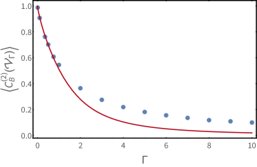
Figure 3: Plot of the escape probability $\braket{C_{B}^{(2)}\left(\mathcal{V}_{\Gamma}\right)}$ as a function of the disorder strength $\Gamma$ for the Lloyd model Hamiltonian $H_{\Gamma}$, as predicted analytically by the heuristic Eq. (24a) (solid line) and the numerical simulations (points). For the case of the numerical simulation, $L\to\infty$ is extrapolated by averaging over disorder for sizes up to $L=2^{12}$. Standard deviations are within the point radius.

We consider the Hamiltonian (18) with i.i.d. on-site energies $\epsilon_{i}$, distributed according to the Cauchy distribution

$$f_{\Gamma}(\epsilon)=\frac{1}{\pi\Gamma}\left[\frac{\Gamma^{2}}{\epsilon^{2}+\Gamma^{2}}\right]\,\;.$$ (50)

The localization length $\xi(E,\Gamma)$ can be calculated by invoking the formula due to Thouless Thouless (1972), which in our notation is

$$\cosh\left(\frac{1}{2\xi(E,\Gamma)}\right)=\frac{\sqrt{(2+E)^{2}+\Gamma^{2}}+\sqrt{(2-E)^{2}+\Gamma^{2}}}{4}\,.$$ (51)

To evaluate Eq. (24a) for this model in the thermodynamic limit, we transition to the continuum limit $\frac{1}{L}\sum_{j}g(E_{j})\mapsto\int dE\rho_{\Gamma}(E)g(E)$. The density of states $\rho_{\Gamma}(E)$ can be obtained easily from the corresponding resolvent, calculated for the Lloyd model in Lloyd (1969), and Eq. (51). The resulting integral is numerically evaluated and yields the data plotted in Figure 3.

Appendix G Comparison of $C_{B}^{(2)}$ and $f_{B}^{(\det)}$

In this section, we will show that

$$P_{\text{return}}=1-C_{B}^{(2)}(\mathcal{V})\geq\left(1-f_{B}^{(\det)}(X_{\mathcal{V}})\right)^{2}\,\;.$$ (52)

Indeed,

$$1-C_{B}^{(2)}(\mathcal{V})=\frac{1}{d}\left\|X_{\mathcal{V}}\right\|_{2}^{2}=\frac{1}{d}\sum_{i}s_{i}^{2}$$

$$\geq\left(\frac{1}{d}\sum_{i}s_{i}\right)^{2}\geq\left[\left(\prod_{i}s_{i}\right)^{\frac{1}{d}}\right]^{2}=\left(1-f_{B}^{(\det)}(X_{\mathcal{V}})\right)^{2}\,\;,$$

where $s_{i}$ denotes the singular values of $X_{\mathcal{V}}$. The first equality follows from the convexity of the mean and the second one from the standard inequality between the arithmetic and geometric mean.

The inequality for the rates Eq. (29) follows by plugging into the inequality (52) the forms (26) and (28).

Appendix H Details of the numerical calculations for MBL

(a) average escape probability (MBL)

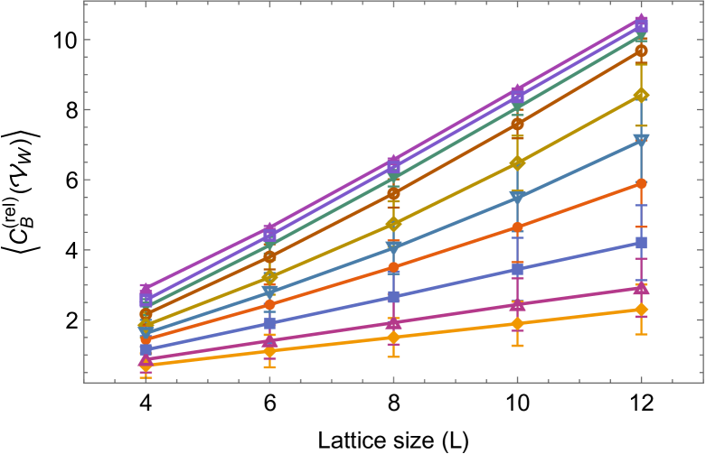
(b) relative entropy CGP (MBL)

Figure 4: Plot of the (a) average escape probability $\braket{C_{B}^{(2)}\left(\mathcal{V}_{W}\right)}$ and (b) $\braket{C_{B}^{(\operatorname{rel})}\left(\mathcal{V}_{W}\right)}$ as a function of the system size $L$ for different values of the disorder strength $W$. The disorder values displayed are $W=0.4,1.0,1.4,1.8,2.5,3.1,3.7,5.0,7.0,9.0$ (monotonically from the top to bottom in the plots) for $L=4,6,\cdots,12$ with sample sizes $$20\,000$,$20\,000$,$20\,000$,$8000$,$2000$$; except at the $W=3.7$, where the sample sizes were doubled. Error bars represent one standard deviation. Entropy has logarithm with base 2.

(a) time-averaged CGP (MBL)

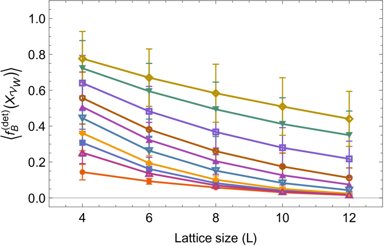
(b) $f_{B}^{(\det)}$ CGP (MBL)

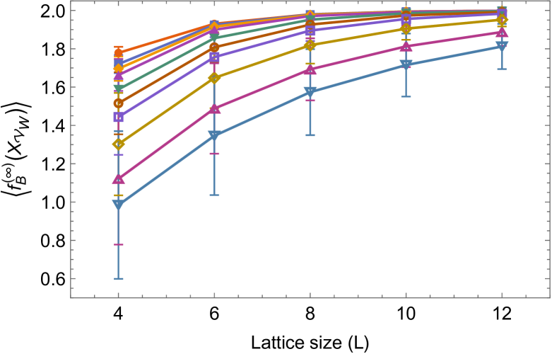
(c) $f_{B}^{(\infty)}$ CGP (MBL)

Figure 5: Plot of the generalized-CGP measures, (a) $\braket{f_{B}^{(\text{time-avg})}\left(X_{\mathcal{V}_{W}}\right)}$, (b) $\braket{f_{B}^{(\text{det})}\left(X_{\mathcal{V}_{W}}\right)}$, and (c) $\braket{f_{B}^{(\infty)}\left(X_{\mathcal{V}_{W}}\right)}$ as a function of the system size $L$ for different values of the disorder strength $W$. The disorder values displayed are $W=0.4,1.0,1.4,1.8,2.5,3.1,3.7,5.0,7.0,9.0$ (monotonically from the top to bottom for (a) and bottom to top for (b)) for $L=4,6,\cdots,12$ with sample sizes $$20\,000$,$20\,000$,$20\,000$,$8000$,$2000$$; except at the $W=3.7$, where the sample sizes were doubled. Error bars represent one standard deviation.

In this section, we list further details of the quantities studied across the ergodic-MBL transition, namely $1-\braket{C_{B}^{(2)}\left(\mathcal{V}_{W}\right)}$, $\braket{C_{B}^{(\operatorname{rel})}\left(\mathcal{V}_{W}\right)}$, $\braket{f_{B}^{(\text{time-avg})}\left(X_{\mathcal{V}_{W}}\right)}$, and $\braket{f_{B}^{(\text{det})}\left(X_{\mathcal{V}_{W}}\right)}$. In Figure 2, we plot the extrapolated rates (for large $L$) as a function of the disorder strength $W$ for the Hamiltonian $H_{\mathrm{XXX}}$ at $h_{x}=0.3$. For this purpose we consider, e.g., for the return probability $1-\braket{C_{B}^{(2)}\left(\mathcal{V}_{W}\right)}$ an ansatz of the form

$$g(L)=\alpha+2^{-\lambda L}\,\;,$$ (53)

where $\alpha$ is the asymptotic value and $\lambda$ is the rate of decay with system size $L$. By performing a nonlinear fit at different disorder values for the various quantities listed above, we found that the $\alpha\approx 0$ (within the uncertainty of the fitting parameters), even for the largest disorder that we consider ($W=9.0$). Therefore, we simplify our ansatz to the form $g(L)\propto 2^{-\lambda L}$ and extract the asymptotic rates by taking the logarithm of the desired quantities.

In Figures 4 and 5 we plot our data for a sample of disorder values and for system sizes $L=4,\cdots,12$. Error bars represent one standard deviation.

Appendix I Coherence-Generating Power and distance in the Grassmannian

Here we present in more detail the underlying differential-geometric structure that is introduced in section V.

Let $\cal H$ denote the finite dimensional Hilbert space of the quantum system and ${\mathcal{B}}({\mathcal{H}})$ the associate operator algebra. The set ${\mathcal{B}}({\mathcal{H}})$ equipped with the Hilbert-Schmidt scalar product $\braket{X,Y}\coloneqq\operatorname*{Tr}\left(X^{\dagger}Y\right)$ turns into a Hilbert space (the space of Hilbert-Schmidt operators) that we will denote by ${\mathcal{H}}_{\operatorname{HS}}$. Superoperators $\cal O$ mapping ${\mathcal{H}}_{\operatorname{HS}}$ into itself can be then endowed with the following norm

$$\|{\cal O}\|_{\operatorname{HS}}\coloneqq\sqrt{{\mathrm{Tr}}_{\operatorname{HS}}({\mathcal{O}}^{\dagger}{\mathcal{O}})}\,\;,$$ (54)

where (a) ${\cal O}^{\dagger}$denotes the Hilbert-Schmidt conjugate of $\mathcal{O}$, i.e., $\braket{\mathcal{O}(X),Y}=\braket{X,\mathcal{O}^{\dagger}(Y)}$ $\forall\,X,Y\in\mathcal{H}_{\operatorname{HS}}$. (b) If $\left\{\ket{i}\right\}_{i=1}^{d}$ is any orthonormal basis of $\mathcal{H}$, one defines ${\mathrm{Tr}}_{\operatorname{HS}}{\mathcal{O}}\coloneqq\sum_{i,j=1}^{d}\braket{\ket{i}\!\bra{j},\mathcal{O}(\ket{i}\!\bra{j})}$.

As we discussed in the main text, instead of invoking orthonormal sequences of kets $\left\{\ket{i}\right\}_{i=1}^{d}$, it is more convenient to work with sets of orthogonal, rank-1 projection operators $B=\left\{P_{i}\coloneqq\ket{i}\!\bra{i}\right\}_{i=1}^{d}$. Let us introduce the space of all such sets over the Hilbert space, which we denote as $\mathcal{M}(\mathcal{H})$. This is essentially the set of all possible orthonormal bases over the Hilbert space once the phase degrees of freedom and ordering have been modded out Zanardi and Campos Venuti (2018a). The elements $B\in\mathcal{M}(\mathcal{H})$ are in one-to-one correspondence with the set of dephasing super-operators, i.e., the map $B\mapsto\mathcal{D}_{B}$ (defined in Eq. (2)) is injective. Given a $B\in{\cal M}_{d}$, the corresponding set of $B$-diagonal operators is

$${\mathcal{A}}_{B}\coloneqq\operatorname*{Span}\left\{P_{i}\right\}_{i=1}^{d}\subset{\mathcal{H}}_{\operatorname{HS}}\,\;,$$ (55)

which is also the range of the $B$-dephasing superoperator ${\cal D}_{B}.$ One can see that Eq. (55) actually defines a Maximally Abelian Sub-Algebra (MASA) of ${\mathcal{H}}_{\operatorname{HS}}$; moreover it can be proven that the set of MASAs of $\mathcal{H}_{\operatorname{HS}}$ can be identified with ${\mathcal{M}}(\mathcal{H})$ (see Zanardi and Campos Venuti (2018a) for a proof). In this way, the set ${\mathcal{M}}(\mathcal{H})$ can be now seen as a subset of the Grassmannian manifold of $d$-dimensional subspaces of ${\mathcal{H}}_{\operatorname{HS}}$. The advantage of this approach is that $\mathcal{M}(\mathcal{H})$ directly inherits the natural metric structure of the Grassmannian

$$D({\mathcal{A}}_{B},{\mathcal{A}}_{B^{\prime}})\coloneqq\left\|{\mathcal{D}}_{B}-{\mathcal{D}}_{B^{\prime}}\right\|_{\operatorname{HS}}\,\;.$$ (56)

We will now connect these concepts to the 2-CGP of unitary quantum maps.

From its definition, $C_{B}^{(2)}(\mathcal{U})$ seems to capture some notion of separation between the sets $B=\left\{P_{i}\right\}_{i=1}^{d}$ and $B^{\prime}=\left\{\mathcal{U}\left(P_{i}\right)\right\}_{i=1}^{d}$. In fact, the $B$-coherence generating power of a unitary map $\mathcal{U}$ is proportional to the (square of the) Grassmannian distance between the input $B$-diagonal algebra ${\cal A}_{B}$ and its image under $\mathcal{U}$ Zanardi and Campos Venuti (2018a). Formally:

$$C^{(2)}_{B}({\mathcal{U}})=\frac{1}{2d}D({\mathcal{A}}_{B},{\cal U}({\mathcal{A}}_{{B}}))^{2}.$$ (57)

where the distance function $D$ is given by (56). The maximum of this function i.e., $\max_{\mathcal{U}}C_{B}^{(2)}(\mathcal{U})=1-1/d$ is achieved for unitary operators $\mathcal{U}$ that connected mutually unbiased bases, namely $\left|\braket{i}{U}{j}\right|=1/d$ ($\forall i,j$), and corresponds to a maximum distance over ${\mathcal{M}}(\mathcal{H})$ given by $D^{\max}=\sqrt{2(d-1)}.$

It is important to stress that, in the light of 4, the Grassmannian distance between MASAs is endowed with a physical meaning in the context of quantum mechanics.

We now turn to establish a connection between the differential structure of $\mathcal{M}(\mathcal{H})$, as induced by the distance function (56), and MBL. One has the natural Riemannian metric over the Grassmannian

$$ds^{2}=D(\Pi,\Pi+d\Pi)^{2}=\operatorname*{Tr}(d\Pi^{2})$$ (58)

($\Pi$ denote the projectors over the $d$-dimensional subspaces comprising the Grassmannian). The latter, in view of Eq. (57), has in turn the physical interpretation as the $C_{B}^{(2)}$ of the unitary associated with an infinitesimal transformation $\left\{\ket{\phi_{i}(\lambda)}\right\}_{i=1}^{d}\mapsto\left\{\ket{\phi_{i}(\lambda+d\lambda)}\right\}_{i=1}^{d}$. The form of the metric (33) follows directly by the calculation of Proposition 6 in Zanardi and Campos Venuti (2018a).

References

- Bohm (1989) D. Bohm, Quantum Theory (Dover Publications, 1989).
- Åberg (2006) J. Åberg, arXiv: quant-ph/0612146 (2006).
- Baumgratz et al. (2014) T. Baumgratz, M. Cramer, and M. B. Plenio, Phys. Rev. Lett. 113, 140401 (2014).
- Streltsov et al. (2017) A. Streltsov, G. Adesso, and M. B. Plenio, Rev. Mod. Phys. 89, 041003 (2017).
- Anderson (1958a) P. W. Anderson, Phys. Rev. 109, 1492 (1958a).
- Lagendijk et al. (2009) A. Lagendijk, B. Van Tiggelen, and D. S. Wiersma, Phys. Today 62, 24 (2009).
- Basko et al. (2006) D. Basko, I. Aleiner, and B. Altshuler, Annals of Physics 321, 1126 (2006).
- Pal and Huse (2010) A. Pal and D. A. Huse, Phys. Rev. B 82, 174411 (2010).
- Nandkishore and Huse (2015) R. Nandkishore and D. A. Huse, Annual Review of Condensed Matter Physics 6, 15 (2015).
- Zanardi and Campos Venuti (2018a) P. Zanardi and L. Campos Venuti, Journal of Mathematical Physics 59, 012203 (2018a).
- Styliaris and Zanardi (2019) G. Styliaris and P. Zanardi, Phys. Rev. Lett. 123, 070401 (2019).
- Prelovšek et al. (2017) P. Prelovšek, M. Mierzejewski, O. Barišić, and J. Herbrych, Annalen der Physik 529, 1600362 (2017).
- Note (1) We note that there exist various proposals for the free operations in the resource theories of coherence (see Chitambar and Gour (2016) for more details). In the following, we will use the term Incoherent Operations for the free operations but, in fact, all results hold for any class that contains Strictly Incoherent Operations Winter and Yang (2016); Yadin et al. (2016).
- Winter and Yang (2016) A. Winter and D. Yang, Phys. Rev. Lett. 116, 120404 (2016).
- Zhao et al. (2018) Q. Zhao, Y. Liu, X. Yuan, E. Chitambar, and X. Ma, Phys. Rev. Lett. 120, 070403 (2018).
- Note (2) We note, however, that the 2-coherence might fail to satisfy the monotonicity property under some classes of free operations.
- Zanardi et al. (2017a) P. Zanardi, G. Styliaris, and L. Campos Venuti, Phys. Rev. A 95, 052306 (2017a).
- Zanardi et al. (2017b) P. Zanardi, G. Styliaris, and L. Campos Venuti, Phys. Rev. A 95, 052307 (2017b).
- Styliaris et al. (2018) G. Styliaris, L. Campos Venuti, and P. Zanardi, Phys. Rev. A 97, 032304 (2018).
- Note (3) In Zanardi et al. (2017a), the measure considered was the uniform over the (whole) simplex of probability distributions, instead of just the extremal ones, resulting in an extra factor .
- Zanardi and Campos Venuti (2018b) P. Zanardi and L. Campos Venuti, Journal of Mathematical Physics 59, 012203 (2018b).
- Marshall et al. (2011) A. W. Marshall, I. Olkin, and B. C. Arnold, Inequalities: Theory of Majorization and Its Applications, Springer Series in Statistics (Springer New York, New York, NY, 2011).
- Reimann (2008) P. Reimann, Phys. Rev. Lett. 101, 190403 (2008).
- Linden et al. (2009) N. Linden, S. Popescu, A. J. Short, and A. Winter, Phys. Rev. E 79, 061103 (2009).
- Campos Venuti and Zanardi (2010) L. Campos Venuti and P. Zanardi, Phys. Rev. A 81, 022113 (2010).
- Campos Venuti et al. (2011) L. Campos Venuti, N. T. Jacobson, S. Santra, and P. Zanardi, Phys. Rev. Lett. 107, 010403 (2011).
- Anderson (1958b) P. W. Anderson, Physical Review 109, 1492 (1958b).
- Luitz and Lev (2017) D. J. Luitz and Y. B. Lev, Annalen der Physik 529, 1600350 (2017).
- Hundertmark (2008) D. Hundertmark, in Analysis and stochastics of growth processes and interface models (2008) pp. 194–219.
- Lloyd (1969) P. Lloyd, Journal of Physics C: Solid State Physics 2, 1717 (1969).
- Thouless (1972) D. J. Thouless, Journal of Physics C: Solid State Physics 5, 77 (1972).
- Abanin et al. (2019) D. A. Abanin, E. Altman, I. Bloch, and M. Serbyn, Rev. Mod. Phys. 91, 021001 (2019).
- Serbyn et al. (2013) M. Serbyn, Z. Papić, and D. A. Abanin, Phys. Rev. Lett. 110, 260601 (2013).
- Luca and Scardicchio (2013) A. D. Luca and A. Scardicchio, EPL (Europhysics Letters) 101, 37003 (2013).
- Goold et al. (2015) J. Goold, C. Gogolin, S. R. Clark, J. Eisert, A. Scardicchio, and A. Silva, Phys. Rev. B 92, 180202 (2015).
- Torres-Herrera and Santos (2015) E. J. Torres-Herrera and L. F. Santos, Phys. Rev. B 92, 014208 (2015).
- Torres-Herrera and Santos (2017) E. J. Torres-Herrera and L. F. Santos, Annalen der Physik 529, 1600284 (2017).
- Serbyn and Abanin (2017) M. Serbyn and D. A. Abanin, Phys. Rev. B 96, 014202 (2017).
- Campos Venuti and Liu (2019) L. Campos Venuti and L. Liu, arXiv:1904.02336 (2019).
- Zanardi and Paunković (2006) P. Zanardi and N. Paunković, Phys. Rev. E 74, 031123 (2006).
- Campos Venuti and Zanardi (2007) L. Campos Venuti and P. Zanardi, Phys. Rev. Lett. 99, 095701 (2007).
- You et al. (2007) W.-L. You, Y.-W. Li, and S.-J. Gu, Phys. Rev. E 76, 022101 (2007).
- Zanardi et al. (2007) P. Zanardi, P. Giorda, and M. Cozzini, Phys. Rev. Lett. 99, 100603 (2007).
- Kolodrubetz et al. (2017) M. Kolodrubetz, D. Sels, P. Mehta, and A. Polkovnikov, Physics Reports 697, 1 (2017).
- Helton et al. (2010) J. S. Helton, K. Matan, M. P. Shores, E. A. Nytko, B. M. Bartlett, Y. Qiu, D. G. Nocera, and Y. S. Lee, Phys. Rev. Lett. 104, 147201 (2010).
- Dai (2015) P. Dai, Rev. Mod. Phys. 87, 855 (2015).
- Hauke et al. (2016) P. Hauke, M. Heyl, L. Tagliacozzo, and P. Zoller, Nature Physics 12, 778 (2016).
- Note (4) The name dynamical conductivity comes from its use when is the (charge) current-current correlation.
- Barišić et al. (2016) O. S. Barišić, J. Kokalj, I. Balog, and P. Prelovšek, Phys. Rev. B 94, 045126 (2016).
- Fishman et al. (1982) S. Fishman, D. R. Grempel, and R. E. Prange, Phys. Rev. Lett. 49, 509 (1982).
- Haake (2010) F. Haake, Quantum Signatures of Chaos, 3rd ed., Springer series in synergetics No. 54 (Springer Berlin, New York, 2010).
- Weinstein et al. (2002) Y. S. Weinstein, S. Lloyd, and C. Tsallis, Phys. Rev. Lett. 89, 214101 (2002).
- Torres-Herrera and Santos (2019) E. J. Torres-Herrera and L. F. Santos, The European Physical Journal Special Topics 227, 1897 (2019).
- Zanardi et al. (2000) P. Zanardi, C. Zalka, and L. Faoro, Phys. Rev. A 62, 030301 (2000).
- (55) N. Anand et. al., in preparation.
- Note (5) A bistochastic matrix is called unistochastic if there exists a unitary matrix such that (see Bengtsson and Życzkowski (2017) for more details).
- Du et al. (2015) S. Du, Z. Bai, and Y. Guo, Phys. Rev. A 91, 052120 (2015).
- Note (6) In fact, the majorization condition is only sufficient for convertibility. It becomes also necessary if an additional condition about the rank of the dephased states is satisfied (see Du et al. (2015) for more details). Nevertheless, if one considers convertibility with some error (arbitrarily small), which is the relevant notion in all physical scenarios, the rank conditions becomes irrelevant.
- Note (7) In light of the connection between infinite time-average and dephasing, this relates to the results in Styliaris et al. (2018), where the question of CGP for dephasing evolutions was investigated.
- Gogolin and Eisert (2016) C. Gogolin and J. Eisert, Reports on Progress in Physics 79, 056001 (2016).
- Cover and Thomas (2012) T. M. Cover and J. A. Thomas, Elements of information theory (John Wiley & Sons, 2012).
- Chitambar and Gour (2016) E. Chitambar and G. Gour, Phys. Rev. A 94, 052336 (2016).
- Yadin et al. (2016) B. Yadin, J. Ma, D. Girolami, M. Gu, and V. Vedral, Phys. Rev. X 6, 041028 (2016).
- Bengtsson and Życzkowski (2017) I. Bengtsson and K. Życzkowski, Geometry of Quantum States: An Introduction to Quantum Entanglement (Cambridge University Press, 2017).