Hardware-friendly Neural Network Architecture for Neuromorphic Computing

Abstract

The hardware-software co-optimization of neural network architectures is becoming a major stream of research especially due to the emergence of commercial neuromorphic chips such as the IBM Truenorth and Intel Loihi. Development of specific neural network architectures in tandem with the design of the neuromorphic hardware considering the hardware constraints will make a huge impact in the complete system level application. In this paper, we study various neural network architectures and propose one that is hardware-friendly for a neuromorphic hardware with crossbar array of synapses. Considering the hardware constraints, we demonstrate how one may design the neuromorphic hardware so as to maximize classification accuracy in the trained network architecture, while concurrently, we choose a neural network architecture so as to maximize utilization in the neuromorphic cores. We also proposed a framework for mapping a neural network onto a neuromorphic chip named as the Mapping and Debugging (MaD) framework. The MaD framework is designed to be generic in the sense that it is a Python wrapper which in principle can be integrated with any simulator tool for neuromorphic chips.

1 Keywords:

neuromorphic computing, neuromorphic chip, hardware constraints, deep learning, hardware-friendly, neural network, crossbar array, convolution, convolutional neural network

2 Introduction

Research in new architectures for convolutional neural networks (CNN) has progressed in various directions so as to fulfil different objectives: smaller deep neural networks Howard et al. (2017); Iandola et al. (2016), low precision neural networks Courbariaux et al. (2016); Rastegari et al. (2016); Zhou et al. (2016) and larger neural networks He et al. (2016) etc. Among these new architectures, the smaller and low precision neural networks are more hardware friendly, in the sense that the entire network maybe mapped onto a neuromorphic chip. These neuromorphic chips are very power efficient as their computations are in spikes, which makes it a good candidate for low power applications in internet of things (IoT), unmanned aerial vehicles (UAVs), robotics and edge computing.

A schematic of a neuromorphic chip is shown in fig 1. The chip has N number of neuromorphic cores. Network on chip (NoC) or router interfaces are not shown for illustration purposes. Each neuromorphic core contains a crossbar array of synapses as shown in the first inset of the figure. The rows and columns of the crossbar correspond to input axons and output neurons respectively. These axons and neurons are interconnected to each other at their intersection. Within each intersection of the crossbar between the word line and the bit line, is a synaptic device which has memory and can perform some in-memory computation (as shown in the second inset). The crossbar architecture is further discussed in subsection 3.3. Considering such a neuromorphic chip, there are several hardware constraints, namely, low bit precision of synaptic weights and output activations Ji et al. (2018), synaptic noise and variability Ambrogio et al. (2014a, b), number of neuromorphic cores, the size of each core size in a neuromorphic core and fan in, fan out degree of each neuron Ji et al. (2018); Gopalakrishnan et al. (2019).

The aim of this paper is as follows:

• to design a hardware friendly deep neural network architecture in order to fit onto a neuromorphic hardware with limited number of cores;

• to maximize the utilization of a single neuromorphic core with limited core size;

• to study how the selected architecture would work with different core sizes, and its corresponding classification accuracy.

Towards this aim, we propose a novel neural network architecture based on existing convolution techniques. We consider a particular architecture to be hardware-friendly so long as it is able to be mapped onto a neuromorphic chip, while achieving a reasonable level of classification accuracy. In this regard, one may take two approaches, either design the network from scratch within the constraints of the neuromorphic hardware specifications or optimise an existing deep network taking into account the hardware specifications. Optimizing an existing deep network can be done by reducing the number of features in each layer so as to fit onto the neuromorphic core without having to split the convolution matrix among different cores. The novel neural network proposed is obtained by extracting different layers from different existing architectures and further modifying the features of some of the layers in these architectures so as to fit onto the neuromorphic hardware.

The paper is organised as follows. Section 3 describes the types of convolutions present in a CNN, a short review of different CNN architectures, MaD framework and computation in a crossbar array. In the subsequent section 4, the proposed architecture is illustrated. Section 5 talks about the results obtained and the paper then concludes with section 6.

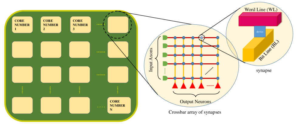
Figure 1: A schematic of a neuromorphic chip with N number of neuromorphic cores. First inset shows the crossbar array of synapses within each core. A memory device is used to implement each synapse at the crossbar intersection (as shown in second inset).

3 Materials and Methods

3.1 Types of convolution used in a convolutional neural network(CNN)

Convolution is an operation that involves the summation of product of terms in two matrices. Convolution and its application in a neural network is to extract the features of the input across each layer of the network. The different convolution techniques applied in a CNN are discussed below.

3.1.1 Standard convolution

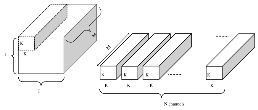
Figure 2: Illustration of the standard convolution.

In the standard convolution, each filter/kernel is multiplied and summed across the whole feature map (input channels). Consider the convolution operation on an input matrix of I $\times$ I $\times$ M with a filter of K $\times$ K $\times$ M (as shown by the dotted lines in fig. 2). This filter operation will give one output feature map which shares filter values for each stride of the convolution. In order to generate N such feature maps, different filters are used, as shown in fig. 2. The computational complexity C of a normal convolution is given as below:

$$C=O^{2}*K^{2}*M*N$$ (1)

where, O = output size after the convolution
K = filter size
M = number of input channels
N = number of output channels

The standard convolution can be computationally intensive and also hard to map onto neuromorphic cores of limited sizes. Therefore, computationally less intensive convolution techniques have been proposed, which include the pointwise convolution, depthwise convolution, flattened convolution, group convolution etc., some of which are further discussed below.

3.1.2 Pointwise convolution

The pointwise convolution is a subset of the standard convolution whereby the filter size per channel is set to 1 $\times$ 1. The entire filter size is hence 1 $\times$ 1 $\times$ M $\times$ N, where M is the number of input channels and N, the number of output channels. Since the filter size is reduced, the computational complexity is also reduced by an order of the square of the filter size. Its computational complexity, C is given as below:

$$C=O^{2}*M*N$$ (2)

where, O = output size after convolution
M = number of input channels
N = number of output channels

3.1.3 Depthwise convolution

In depthwise convolution, the convolution is independently applied to each input channel so as to obtain its corresponding output feature map. Hence, in depthwise convolution, the summation operation is applied within each corresponding input channel. After the depthwise convolution operation, the number of output channels obtained is the same as that of the number of input channels. One may however also increase the number of output channels per input channel using a depth multiplier.

As shown in fig. 3, the input matrix is convolved with M different filters, each of size K $\times$ K. The output of each depthwise convolution involving a filter and a single input channel is O $\times$ O $\times$ 1, and M such filters compute an output of dimensions O $\times$ O $\times$ M. The depth multiplier is set to one here. The computational complexity, C of the depthwise convolution considering depth multiplier is given as below:

$$C=O^{2}*K^{2}*M*D$$ (3)

where, O = output size after convolution
K = filter size
M = number of input channels
D = depth multiplier

The application of the depthwise convolution, then pointwise convolution together, is known as the depthwise separable convolution. Depthwise separable convolution is used extensively in MobileNets Howard et al. (2017).

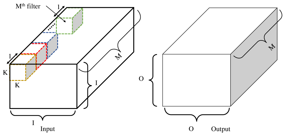
Figure 3: Illustration of the depthwise convolution. Note that the depth multiplier is set to one here.

3.1.4 Grouped convolution

Grouped convolution is another convolution technique whereby the standard convolution is applied separately to an input matrix diced into equal parts along its channel axis. As shown in fig. 4, the input channels and filters are divided into several equal parts along the channel axis. All the separate output features of these independent parts are then combined into a final output. Depending on how the parts are combined, different variations of the grouped convolutions include: stacked convolution, dependent stacked convolution and shuffled convolution. Computational complexity of the grouped convolution is calculated as per the standard convolution but grouped convolutions are more neuromorphic hardware friendly as each neuron has a lower fan in/fan out degree when mapped onto a crossbar array of synapses.

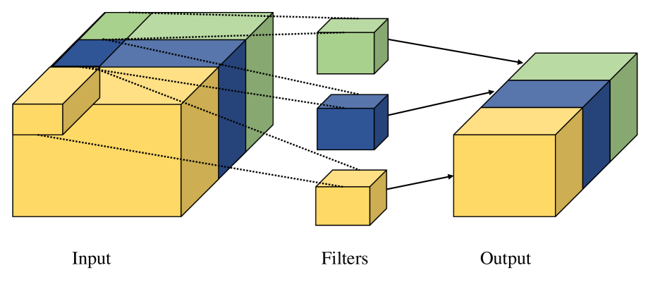
Figure 4: Illustration of grouped convolution.

3.2 Different convolutional neural networks

This subsection briefly introduces several popular CNNs. These are some of the CNNs we have studied whilst proposing the novel CNN architecture that is more hardware-friendly.

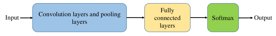
Figure 5: Block diagram illustration of the AlexNet and VGGNet.

3.2.1 AlexNet

Geoffrey Hinton and team introduced the first deep neural network architecture, Alexnet, which was named after his student. AlexNet Krizhevsky et al. (2012) paved the way for a new field of artificial intelligence research known as deep learning. Deep learning has since been applied to many fields in AI, with state-of-the-art results Graham (2014); Clevert et al. (2015); Wan et al. (2013). Figure 5 details the architecture of the AlexNet in a block diagram. AlexNet is a CNN with alternate convolutional and pooling layers, ending with fully connected layers.

3.2.2 VGGNet

VGGNet Simonyan and Zisserman (2014) was introduced by the Visual Graphics Group at Oxford. VGGNet is similar to AlexNet, with slight modification in the placement of layers. The architecture is deeper compared to AlexNet, and retains the input width in the early layers. Figure 5 is also representative of the VGGNet architecture. We note that in VGGNet, the pooling layers are applied after every two convolution layers in the beginning of the architecture and every three layers afterwards. This technique preserves the larger width of the layers at the beginning of the architecture. VGGNet uses three layers of full connections before the softmax classifier.

3.2.3 GoogLeNet

GoogLeNet Szegedy et al. (2015) is a 22 layer deep CNN. Its main novelty is the inception module, which concatenates the output of several convolutions of the same activations from the previous layer. Figure 6 shows the blockwise architecture of the GoogLeNet and the inception module in the inset. GoogLeNet started using 1$\times$1 convolution or pointwise convolution extensively in their inception modules, which was introduced in Lin et al. (2013). It is the winner of the ILSVRC 2014 classification challenge which involves classifying the IMAGENET dataset Deng et al. (2009).

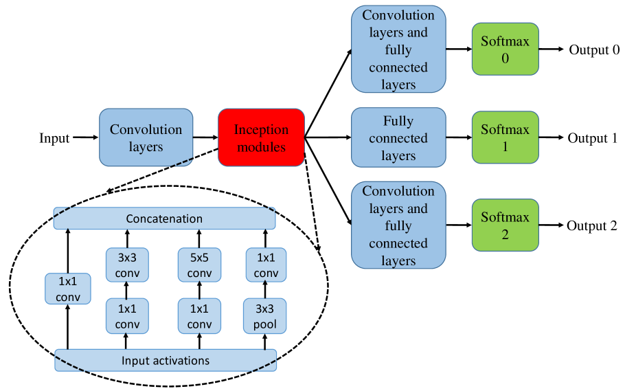
Figure 6: Block diagram illustration of GoogLeNet.

3.2.4 SqueezeNet

SqueezeNet Iandola et al. (2016) is another architecture similar to MobileNet with an even smaller size. One of the compressed versions of SqueezeNet has only 0.47MB of parameters, making it ideal for deployment on a mobile platform. SqueezeNet has a fire module, consisting of a squeezing network module followed by an expanding network module. Fire module is the key to preserving classification accuracy while reducing network size. Figure 7 shows the details of the SqueezeNet architecture. It does not have any fully connected layers before the softmax classifier, in contrast to AlexNet and VGGNet.

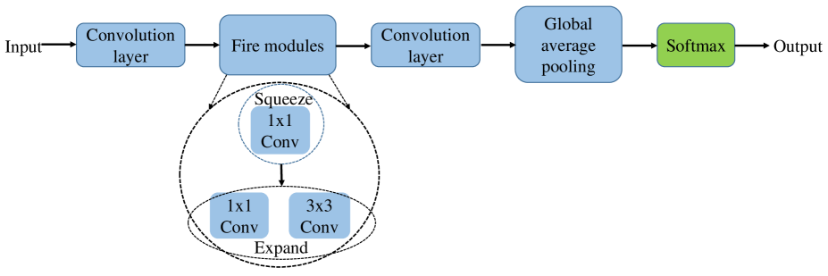
Figure 7: Block diagram illustration of SqueezeNet.

3.2.5 MobileNet

MobileNet Howard et al. (2017) was proposed by Google, with the main motivation of reducing the the network size and its parameters. MobileNet uses depthwise separable convolution as illustrated in the previous section 3.1. Figure 8 shows the architecture of the MobileNet. It is also more neuromorphic hardware-friendly as the fan in/fan out connections of each neuron is much less, as a result of the pointwise and depthwise convolutions.

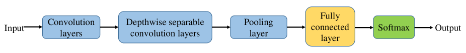
Figure 8: Block diagram illustration of MobileNet.

3.3 Crossbar array of synapses

The neuromorphic chip discussed in this paper is based on a crossbar architecture Prezioso et al. (2015) of non-volatile memory synapses. In Fig. 1, the first inset shows a crossbar architecture of synapses in a neuromorphic chip. For a biological neuron, an axon connects the pre-synaptic neuron to the synapse, which is the site of connection between the axon of the pre-synaptic neuron and the dendrite of the post-synaptic neuron. Similarly, in CNNs on a neuromorphic hardware, the synapse can be viewed as the site of connections between the input neurons and output neurons of a convolution layer. Memory device is used to represent these synaptic weights which are analogous to the weights in the filters of the CNNs (Fig. 1, second inset). In the mesh-like crossbar array, the synapse of the neuromorphic core establish connections between axons and neurons of that neuromorphic core. Typically in a neuromorphic chip, spiking neurons are used to integrate the current from the synapses and a spike is emitted, when the firing threshold is met. Hence, each neuron at the bottom of the crossbar array performs a nonlinear function on the convolution operation between input and synaptic weights. These operations are also termed as matrix dot vector multiplications (MVM) Hu et al. (2016).

3.4 Python wrapper: MaD Framework

One of the main challenges in the field of neuromorphic hardware is to efficiently map the neurons in a CNN onto the neuromorphic chip while fulfilling hardware constraints such as core size, number of cores and fan-in/fan-out Ji et al. (2016). Existing neuromorphic chips have a mapping framework which is hardware specific. IBM’s TrueNorth chip Akopyan et al. (2015) uses Corelet language Amir et al. (2013) based on MATLAB, a programming language specific to their hardware. Within this MATLAB framework, a mapping technique is integrated as a minimization problem Akopyan et al. (2015). SpiNNaker and BrainScaleS uses a simulator-independent language, PyNN P et al. (2009), based on Python. Sequential mapping is used in SpiNNaker. Neural engineering framework (NEF) is developed for Neurogrid Voelker et al. (2017). Neutrams Ji et al. (2016) addresses an optimized mapping technique based on graph partition problem: Kernighan-Lin (KL) partitioning strategy for network on chip (NoC). Even though, every neuromorphic hardware simulator tool provides certain mapping techniques, optimized mapping onto a single neuromorphic core is often neglected and is relatively unexplored. While developing deep neural networks that are to be mapped onto a neuromorphic chip, one need not in principle be aware of the underlying hardware constraints of the chip. However, to better utilize the chip for a classification task, software and hardware co-design is encouraged, which requires the neural network designer to be aware of the underlying hardware constraints. The aforementioned issues are addressed using the MaD framework. The MaD framework is a generic Python wrapper which has an optimized algorithm for mapping a feed-forward neural network such as the MLP, CNN and spiking neural network (SNN) onto a crossbar array of synapses with corresponding synaptic weights, thereby fitting the neurons using the least number of neuromorphic cores. The Python wrapper is also suitable as a debugging tool for verification of inferencing results after mapping the neural network architectures onto the neuromorphic chip. Thus, together the framework is called the mapping and debugging (MaD) framework. This Python wrapper is developed in connection with the simulator in Lee et al. (2018), which shares several similar techniques to that of Neutrams Ji et al. (2016).

The functionalities of the MaD framework is explained in the flowchart (fig. 9). Given a CNN chosen for a classification or detection task, its hyper-parameters such as filter size, strides and padding at each layer is known. The chosen network is trained using existing deep learning frameworks and the trained weight variables (together with the above-mentioned hyper-parameters) are input into the mapping function. Core utilization is defined as the number of axons and neurons utilized in a single neuromorphic core, represented as [axons $\times$ neurons]. Core utilization, as shown in the flowchart, is output from another function which calculates the number of axons and the number of neurons used for mapping a section of a particular layer onto a single core. The mapping of different portions of a convolutional layer onto different cores is shown in the fig. 10. Different colors within the layer show that these neurons are mapped onto different cores. For example, neurons in yellow are mapped onto core 1 and neurons in brown are mapped onto core 10 etc. The details of the mapping function, core utilization and padding techniques are given in subsequent subsections. The supplementary material contains the discussion on the optimizations performed during mapping.

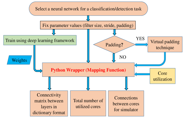
Figure 9: Flowchart of Python wrapper: Details of the Python wrapper shown in a flowchart, with the input and output of the mapping function shown. Core utilization and weight files are in different color to denote that these inputs are results from other functions.

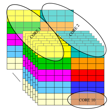
Figure 10: Division of a CNN layer into different neuromorphic cores.

3.4.1 Mapping Function

The mapping function is the core of the Python wrapper. Fig. 9 also shows the input and output of the mapping function. The inputs to mapping function are input size, filter size, stride, padding, core utilization and weight files. The input size is the size of the input datasets, for eg. 28$\times$28 in the case of MNIST or 32$\times$32 in the case of CIFAR-10. Filter size is the size of filters used for each convolution layer. For instance, it is 3$\times$3 throughout all convolutional layers in the CNNs described in result subsection given in supplementary material. Stride and padding are layer-specific. The detailed calculation of the core utilization is discussed in subsection 3.4.2. Weight files are the weights obtained after training the deep network. The output section in fig. 9 shows the outputs of the mapping function. There are mainly three outputs, a connectivity matrix for verifying the interconnectivity between the cores and within the core, to verify the cores utilized and an automated generation of connection list for simulator.

The steps for mapping are as follows:

• Name the neurons using the convention: L1-F1-N[1,1], which implies layer:1, feature map:1, and neuron in row:1 and column:1.

• Create a connectivity list stating how populations of neurons in one layer are connected to populations in the previous layer.

• Choose a population of neurons from a particular layer, based on the core utilization, to be mapped on to a particular core.

• Repeat step 3 until all neurons are mapped onto a core. Since the naming and connectivity list are determined at the beginning, the neurons and axons are automatically duplicated across cores during mapping.

3.4.2 Core Utilization

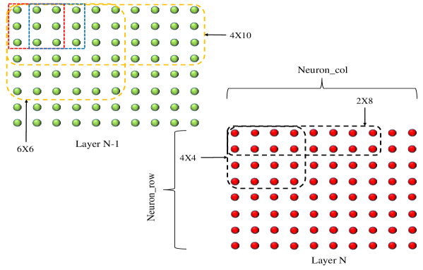
Figure 11: Two layers of the convolution operation to illustrate optimization of core utilization. Layer N-1 neurons are in green, while layer N neurons are in red. Synaptic connections are shown for two neurons in layer N.

Consider two layers of a CNN as shown in fig. 11. First two neurons in layer N (in red) are connected to layer N-1 neurons (in green) with the synaptic connections as shown with their respective afferent neurons in red and blue squares. Size of the convolution filter used is 3$\times$3. The synaptic connections extend across the layers as per the kernel size and strides used during convolution. While mapping these two layers in fig. 11 onto a core with crossbar array, the green neurons in layer N-1 will be the axons and the red neurons in layer N will be the neurons as in fig. 1 (notice the overlap of filter kernel as it traverses across the layer N-1). These overlapping green neurons may however be mapped onto the axons of the crossbar array without duplicates. Duplication of axons is not desirable. Duplication of axons while mapping onto a neuromorphic core will require an input to be duplicated into multiple axons within a neuromorphic core (increases core usage). Hence, the toeplitz matrix method is utilized for efficient mapping of these convolution layers onto a neuromorphic core Appuswamy et al. (2016) Gray (2006). For a given mapping on a particular core, the core utilization maybe calculated based on the number of neurons and axons connected together. The number of axons can be evaluated as an algorithmic condition in the mapping function as there are overlapping axons whereas neurons selection become bit straight forward. The overlapping axons are defined as the axons (in layer N-1) which share connections with more than a single neuron (in layer N), the term overlapping is because of the overlapping nature of the axons with the neighbourhood of the kernel filter with respect to strides (see layer N-1 in fig. 11, the overlapping axons from the red and blue dotted squares are 6). Depending on this overlap, kernel filter size and strides, the total number of axons to be selected is given by the below equation:

$$N\_axons=K*K+K*S(Neuron\_col-1)+$$ (4)

$$S*S(Neuron\_col-1)(Neuron\_row-1)+$$

$$K*S(Neuron\_row-1)$$

Where,
$N\_axons$ = total number of axons to be selected
K = convolution kernel filter size
S = stride
$Neuron\_row$ = number of neurons across row
$Neuron\_col$ = number of neurons across column
The selection of neurons, $Neuron\_row$ and $Neuron\_col$, in a layer has to satisfy the condition: number of axons, $N\_axons$ $<=$ number of physical axons (eg. 256 or 512 or 1024) in the neuromorphic core. Eq. 4 considers only a single feature map; this can be easily extended to multiple feature maps by multiplying with the respective number of feature maps.

3.5 Computation in a crossbar array

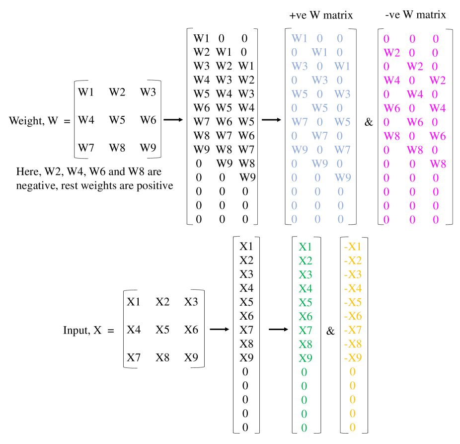
Figure 12: Division of network parameters, weights and input activations into positive and negative matrices.

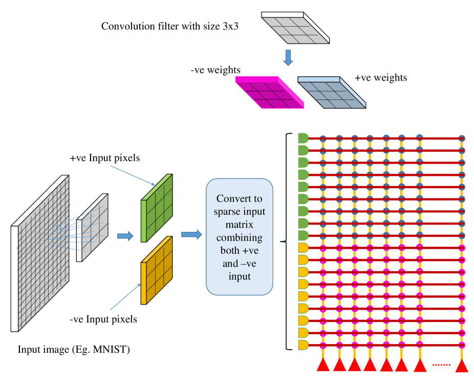
Figure 13: Computation in a crossbar architecture within a single neuromorphic core.

The crossbar array of synapses in a neuromorphic chip is capable of doing convolutions. Mathematically, convolution is the sum of dot product of two input matrices. One matrix being the input matrix and the another is the filter matrix as shown in fig. 12. In CNNs, the input matrix will be the activations from the prior layer while the filter matrix is the convolution filter kernel, saved as weights, W after a CNN is trained. Since these weights can be either positive or negative values after training, one way of implementing convolution on a crossbar array is to split the weights into positive and negative matrices along with two copies of input matrices in positive and negative values. The details of the matrix generation is shown in fig. 12, which incorporate the convolution operation in crossbar arrays as described in Yakopcic et al. (2016) (also referred in our previous paper Gopalakrishnan (2019)). Single column of crossbar gives the output of a convolution operation, which is the output of corresponding neuron. Convolution operation is extended to multiple columns of RRAM synapses to compute in parallel. This requires the weights and inputs to be represented in a toeplitz matrix, as shown in fig. 12. Yakopcic et al. (2017) illustrated such an implementation in fig. 13. This implementation doubles the utilization of hardware resources which is similar to IBM Truenorth Esser et al. (2016), where they need two synapses to implement the ternary weights (-1, 0, +1).

In order to mitigate the above described double synaptic utilization in a neuromorphic hardware, one can implement two memory devices at each synapse to represent both positive and negative weights by subtraction. This implementation does not need to partition the weights and inputs into positive and negative matrices instead, generating a toeplitz matrix is sufficient.

4 Proposed architecture

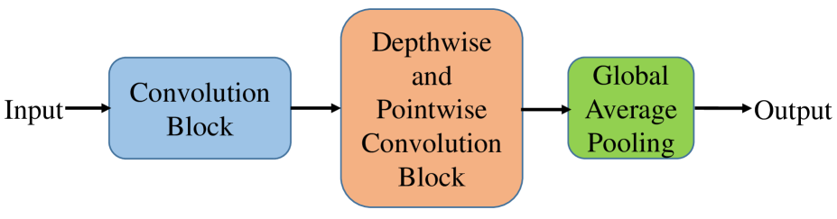
Figure 14: The proposed hardware-friendly neural network architecture in block diagram.

The proposed architecture borrows from the different CNNs discussed in section 3.2. It is a hybrid combination of the VGGNet, MobileNet and SqueezeNet. As shown in fig. 14, the first three layers are convolutional layers as in the case of VGGNet (convolutional block) and the next layers are alternate layers of Depthwise and Pointwise convolutions (Depthwise and Pointwise convolutional block) as in the case of MobileNet. Since the fully connected layers require more parameters and have large fan in/fan out degrees, the last fully connected layer of MobileNet is replaced with global average pooling, similar to the SqueezeNet architecture. Pooling layers are not necessary in a CNN. It can be replaced by using convolutional layers with stride of 2 so as to achieve dimension reduction without significant loss in accuracy, even though mathematically, they are different Springenberg et al. (2014). Thus, the proposed architecture is novel whereby it does not have pooling and fully connected layers. The detailed input size and output size of each layer of the proposed architecture for different core sizes are given in table 1.

Table 1: Neural network architecture (NN archi.) for different core sizes

NN	Core Size
archi.	256$\times$256		512$\times$512		1024$\times$1024
Layers	Input Size	Output Size	Input Size	Output Size	Input Size	Output Size
Conva	224$\times$224$\times$3	112$\times$112$\times$16	224$\times$224$\times$3	112$\times$112$\times$32	224$\times$224$\times$3	112$\times$112$\times$32
Conv	112$\times$112$\times$16	56$\times$56$\times$28	112$\times$112$\times$32	56$\times$56$\times$56	112$\times$112$\times$32	56$\times$56$\times$64
Conv	56$\times$56$\times$28	28$\times$28$\times$64	56$\times$56$\times$56	28$\times$28$\times$256	56$\times$56$\times$64	28$\times$28$\times$256
Db	28$\times$28$\times$64	28$\times$28$\times$64	28$\times$28$\times$256	28$\times$28$\times$256	28$\times$28$\times$256	28$\times$28$\times$256
Pc	28$\times$28$\times$64	28$\times$28$\times$256	28$\times$28$\times$256	28$\times$28$\times$256	28$\times$28$\times$256	28$\times$28$\times$256
D	28$\times$28$\times$256	14$\times$14$\times$256	28$\times$28$\times$256	14$\times$14$\times$256	28$\times$28$\times$256	14$\times$14$\times$256
P	14$\times$14$\times$256	14$\times$14$\times$256	14$\times$14$\times$256	14$\times$14$\times$512	14$\times$14$\times$256	14$\times$14$\times$512
D	14$\times$14$\times$256	14$\times$14$\times$256	14$\times$14$\times$512	14$\times$14$\times$512	14$\times$14$\times$512	14$\times$14$\times$512
P	14$\times$14$\times$256	14$\times$14$\times$256	14$\times$14$\times$512	14$\times$14$\times$512	14$\times$14$\times$512	14$\times$14$\times$512
D	14$\times$14$\times$256	14$\times$14$\times$256	14$\times$14$\times$512	14$\times$14$\times$512	14$\times$14$\times$512	14$\times$14$\times$512
P	14$\times$14$\times$256	14$\times$14$\times$256	14$\times$14$\times$512	14$\times$14$\times$512	14$\times$14$\times$512	14$\times$14$\times$512
D	14$\times$14$\times$256	14$\times$14$\times$256	14$\times$14$\times$512	14$\times$14$\times$512	14$\times$14$\times$512	14$\times$14$\times$512
P	14$\times$14$\times$256	14$\times$14$\times$256	14$\times$14$\times$512	14$\times$14$\times$512	14$\times$14$\times$512	14$\times$14$\times$512
D	14$\times$14$\times$256	14$\times$14$\times$256	14$\times$14$\times$512	14$\times$14$\times$512	14$\times$14$\times$512	14$\times$14$\times$512
P	14$\times$14$\times$256	14$\times$14$\times$256	14$\times$14$\times$512	14$\times$14$\times$512	14$\times$14$\times$512	14$\times$14$\times$512
D	14$\times$14$\times$256	14$\times$14$\times$256	14$\times$14$\times$512	14$\times$14$\times$512	14$\times$14$\times$512	14$\times$14$\times$512
P	14$\times$14$\times$256	14$\times$14$\times$256	14$\times$14$\times$512	14$\times$14$\times$512	14$\times$14$\times$512	14$\times$14$\times$512
D	14$\times$14$\times$256	7$\times$7$\times$256	14$\times$14$\times$512	7$\times$7$\times$512	14$\times$14$\times$512	7$\times$7$\times$512
P	7$\times$7$\times$256	7$\times$7$\times$1000	7$\times$7$\times$512	7$\times$7$\times$1000	7$\times$7$\times$512	7$\times$7$\times$1000
D	7$\times$7$\times$1000	7$\times$7$\times$1000	7$\times$7$\times$1000	7$\times$7$\times$1000	7$\times$7$\times$1000	7$\times$7$\times$1000
P	7$\times$7$\times$1000	7$\times$7$\times$1000	7$\times$7$\times$1000	7$\times$7$\times$1000	7$\times$7$\times$1000	7$\times$7$\times$1000
aConvolution layer.
bDepthwise convolution layer.
cPointwise convolution layer.

5 Result

In this section, we design three sets of experiments to investigate how variations in the proposed architecture affect classification accuracies on the IMAGENET dataset Deng et al. (2009). Note that all the different neural network models considered in this section is illustrated in the supplementary material. The first set of experiment investigates the performance of the proposed architecture with and without pooling layers and fully connected layers. The proposed architecture as in table 1 for the core size of 1024$\times$1024 (we refer this as base model in the entire manuscript) is trained on the IMAGENET dataset with and without pooling layers, similarly with and without fully connected layers. Network without pooling layer is exactly same as the mentioned architecture in table 1, but for network with pooling layer, all the layers with stride of 2 is inserted with pooling layers. Fully connected layer of size 1024$\times$1000 is added at the end of the proposed architecture in network with fully connected layer. From table 2, it can be seen that there is no significant improvement in classification accuracies with and without pooling layers and fully connected layers. Hence, we have completely removed the pooling layers and fully connected layers from the proposed architecture.

The proposed architecture is trained on IMAGENET dataset with batch normalization technique before ReLU activation function in every layer. We would consider binary activations in future work, as the purpose of this work is to propose a novel CNN architecture that is neuromorphic hardware-friendly. Hence, how quantized activations affect classification accuracies is beyond the scope of our current work. The network does not converge without batch normalization. For the next set of experiments, there are three architectures for three different core sizes as mentioned in table 1. IMAGENET dataset is trained on all the three different architectures. From table 3, it can be seen that the classification accuracy for different architectures improve with bigger neuromorphic core sizes, as larger network architectures can be mapped onto larger core sizes.

The third set of experiment involves addition of layers on top of the base model as proposed in table 1 for the core size of 1024$\times$1024. Here, we have considered adding three layers (depthwise and pointwise convolution layer, standard convolution layer and fully connected layers) separately on to the base model to test the accuracy on IMAGENET dataset. For the addition of depthwise and pointwise convolution layers (1 DP layer as in table 4), we have added one depthwise and one pointwise convolution respectively to the end of the base model and trained the network on IMAGENET dataset. For the addition of a standard convolution layer (1 Conv layer as in table 4), we have added a convolution layer to the front of the base model. Similarly, for the addition of fully connected layer (2 FC layer as in table 4), we have added 2 fully connected layer at the end of the base model. For this, we changed the output size of the last pointwise convolution layer to $7\times 7\times 1024$, instead of $7\times 7\times 1000$. Note that adding fully connected layer will increase fan-in degree and will not fit onto 1024 core, i.e. fully connected layer is not a hardware-friendly layer. 1 DP-1 Conv layer as in table 4 is the addition of both depthwise and pointwise convolution layer at the end of the base model along with the addition of convolution layer at the front of the base model. Table 4 shows the results for addition of layers to the base model. It can be seen that all the accuracies are more than the accuracy of the base model which is 68.14$\%$ as given in table 2. Adding a standard convolution layer at the front of the base model gives better result than adding a depthwise and pointwise convolution layer at the end of the base model. Whereas, adding two fully connected layers at the end of the base model does not show much improvement in accuracy as in the aforementioned case of addition of single layers. But, addition of both depthwise-pointwise convolution layer along with standard convolution layer shows the best result among the four, which is around the same accuracy claimed by VGGNET.

Table 2: With and without pooling and fully connected layers

Classification Accuracy (%)
Base model∗	With pooling layer	With FC∗∗ layer
68.14	68.85	68.21
∗The proposed architecture as in table 1 for the core size of 1024$\times$1024.
∗∗Fully connected.

Table 3: Using different architectures for different core sizes

Classification Accuracy (%)
256$\times$256	512$\times$512	1024$\times$1024
62.46	67.78	68.14

Table 4: Addition of layers to base model

Classification Accuracy (%)
1 DP∗ layer	1 Conv layer	1 DP-1 Conv layer	2 FC layer
68.73	69.43	70.186	68.21
∗Depthwise and Pointwise convolution.

6 Conclusion

Neuromorphic hardware friendly neural networks are customized for a specific neuromorphic hardware such that it can then be easily mapped onto the hardware. In our work, the proposed neuromorphic hardware friendly CNN is compatible with a neuromorphic hardware with crossbar array of synapses in a neuromorphic core. One of the motivation of the proposed architecture is to maximise the utilization of the crossbar architecture, which may not be possible with existing CNNs, but we can then modify to fit onto the hardware. By doing so, we avoid splitting the weight matrix of a particular neuron into more than one core during mapping. Splitting requires intermediate neurons which increase the hardware overhead and also effectively introduces new non-linearity into the neural network which affects accuracies. Also mapping of the existing CNNs onto the neuromorphic chip requires more than one neuromorphic chip with limited cores. The deeper layers in the existing CNNs with bigger feature maps also require splitting the weight matrix. This splitting of weight matrix is completely removed in our proposed hardware friendly architecture.

Different architectures for different neuromorphic core sizes in the results further shows that the architecture can be tailored for different core sizes. It also shows that larger the core size, the larger the network, and the better the classification accuracy. Chip design however limits the size of the neuromorphic cores. We have proposed a novel architecture without pooling and fully connected layers. The results in the section 5 further justifies not using the aforementioned layers as classification accuracies are not affected.

In our current study, we only studied CNNs that do not have connections skipping layers. Hence, residual networks He et al. (2016) are not considered. Skipped connections would increase the fan-in/fan-out degree of the neurons in a neuromorphic chip. We would consider mapping of such networks in a future work. We would also consider other hardware constraints such as low precision of weights and binary activations in the future. For Resistive Random Access Memory (RRAM) devices, synaptic noise and variability will have to be considered as well.

Author Contributions

The first and second author designed and proposed the architecture and experimental framework. The first author wrote the manuscript; the second author edited the manuscript and conducted some experiments. The third author is involved in generating the figures and conducting some experiments.

Funding

This research is supported by Programmatic grant no. A1687b0033 from the Singapore governments Research, Innovation and Enterprise 2020 plan (Advanced Manufacturing and Engineering domain).

References

- Akopyan et al. (2015) Akopyan, F., Sawada, J., Cassidy, A., Alvarez-Icaza, R., Arthur, J., Merolla, P., et al. (2015). Truenorth: Design and tool flow of a 65 mw 1 million neuron programmable neurosynaptic chip. IEEE Transactions on Computer-Aided Design of Integrated Circuits and Systems 34, 1537–1557
- Ambrogio et al. (2014a) Ambrogio, S., Balatti, S., Cubeta, A., Calderoni, A., Ramaswamy, N., and Ielmini, D. (2014a). Statistical fluctuations in hfox resistive-switching memory: Part i - set/reset variability. IEEE Transactions on Electron Devices 61, 2912–2919. 10.1109/TED.2014.2330200
- Ambrogio et al. (2014b) Ambrogio, S., Balatti, S., Cubeta, A., Calderoni, A., Ramaswamy, N., and Ielmini, D. (2014b). Statistical fluctuations in hfox resistive-switching memory: Part ii - random telegraph noise. IEEE Transactions on Electron Devices 61, 2912–2919. 10.1109/TED.2014.2330200
- Amir et al. (2013) Amir, A., Datta, P., Risk, W. P., Cassidy, A. S., Kusnitz, J. A., Esser, S. K., et al. (2013). Cognitive computing programming paradigm: A corelet language for composing networks of neurosynaptic cores. In The 2013 International Joint Conference on Neural Networks (IJCNN). 1–10
- Appuswamy et al. (2016) Appuswamy, R., Nayak, T. K., Arthur, J. V., Esser, S. K., Merolla, P., McKinstry, J. L., et al. (2016). Structured convolution matrices for energy-efficient deep learning
- Clevert et al. (2015) Clevert, D., Unterthiner, T., and Hochreiter, S. (2015). Fast and accurate deep network learning by exponential linear units (elus). CoRR abs/1511.07289
- Courbariaux et al. (2016) Courbariaux, M., Hubara, I., Soudry, D., El-Yaniv, R., and Bengio, Y. (2016). Binarized neural networks: Training deep neural networks with weights and activations constrained to+ 1 or-1. arXiv preprint arXiv:1602.02830
- Deng et al. (2009) Deng, J., Dong, W., Socher, R., Li, L.-J., Li, K., and Fei-Fei, L. (2009). ImageNet: A Large-Scale Hierarchical Image Database. In CVPR09
- Esser et al. (2016) Esser, S. K., Merolla, P. A., Arthur, J. V., Cassidy, A. S., Appuswamy, R., Andreopoulos, A., et al. (2016). Convolutional networks for fast, energy-efficient neuromorphic computing. Proceedings of the National Academy of Sciences 113, 11441–11446. 10.1073/pnas.1604850113
- Gopalakrishnan (2019) Gopalakrishnan, R. (2019). Rram based neuromorphic algorithms
- Gopalakrishnan et al. (2019) Gopalakrishnan, R., Kumar, A. J. S., and Chua, Y. (2019). Mad: Mapping and debugging framework for implementing deep neural network onto a neuromorphic chip with crossbar array of synapses
- Graham (2014) Graham, B. (2014). Fractional max-pooling. CoRR abs/1412.6071
- Gray (2006) Gray, R. M. (2006). Toeplitz and circulant matrices: A review
- He et al. (2016) He, K., Zhang, X., Ren, S., and Sun, J. (2016). Deep residual learning for image recognition. In Proceedings of the IEEE conference on computer vision and pattern recognition. 770–778
- Howard et al. (2017) Howard, A. G., Zhu, M., Chen, B., Kalenichenko, D., Wang, W., Weyand, T., et al. (2017). Mobilenets: Efficient convolutional neural networks for mobile vision applications. arXiv preprint arXiv:1704.04861
- Hu et al. (2016) Hu, M., Strachan, J. P., Li, Z., Grafals, E. M., Davila, N., Graves, C., et al. (2016). Dot-product engine for neuromorphic computing: Programming 1t1m crossbar to accelerate matrix-vector multiplication. In 2016 53nd ACM/EDAC/IEEE Design Automation Conference (DAC). 1–6
- Iandola et al. (2016) Iandola, F. N., Han, S., Moskewicz, M. W., Ashraf, K., Dally, W. J., and Keutzer, K. (2016). Squeezenet: Alexnet-level accuracy with 50x fewer parameters and¡ 0.5 mb model size. arXiv preprint arXiv:1602.07360
- Ji et al. (2018) Ji, Y., Zhang, Y., Chen, W., and Xie, Y. (2018). Bridge the gap between neural networks and neuromorphic hardware with a neural network compiler. In Proceedings of the Twenty-Third International Conference on Architectural Support for Programming Languages and Operating Systems (ACM), 448–460
- Ji et al. (2016) Ji, Y., Zhang, Y., Li, S., Chi, P., Jiang, C., Qu, P., et al. (2016). Neutrams: Neural network transformation and co-design under neuromorphic hardware constraints. In 2016 49th Annual IEEE/ACM International Symposium on Microarchitecture (MICRO). 1–13
- Krizhevsky et al. (2012) Krizhevsky, A., Sutskever, I., and Hinton, G. E. (2012). Imagenet classification with deep convolutional neural networks. In Advances in neural information processing systems. 1097–1105
- Lee et al. (2018) Lee, M., Cui, Y., Somu, T., Luo, T., Zhou, J., Tang, W., et al. (2018). A system-level simulator for rram-based neuromorphic computing chips
- Lin et al. (2013) Lin, M., Chen, Q., and Yan, S. (2013). Network in network. CoRR abs/1312.4400
- P et al. (2009) P, D. A., Daniel, B., Jochen, E., Jens, K., Eilif, M., Dejan, P., et al. (2009). Pynn: A common interface for neuronal network simulators 2, 11. 10.3389/neuro.11.011.2008
- Prezioso et al. (2015) Prezioso, M., Merrikh-Bayat, F., Hoskins, B. D., Adam, G. C., Likharev, K. K., and Strukov, D. B. (2015). Training and operation of an integrated neuromorphic network based on metal-oxide memristors 521, 61–64
- Rastegari et al. (2016) Rastegari, M., Ordonez, V., Redmon, J., and Farhadi, A. (2016). Xnor-net: Imagenet classification using binary convolutional neural networks. In European Conference on Computer Vision (Springer), 525–542
- Simonyan and Zisserman (2014) Simonyan, K. and Zisserman, A. (2014). Very deep convolutional networks for large-scale image recognition. arXiv preprint arXiv:1409.1556
- Springenberg et al. (2014) Springenberg, J. T., Dosovitskiy, A., Brox, T., and Riedmiller, M. A. (2014). Striving for simplicity: The all convolutional net. CoRR abs/1412.6806
- Szegedy et al. (2015) Szegedy, C., Liu, W., Jia, Y., Sermanet, P., Reed, S., Anguelov, D., et al. (2015). Going deeper with convolutions. In Computer Vision and Pattern Recognition (CVPR), 2015 IEEE Conference on (IEEE), 1–9
- Voelker et al. (2017) Voelker, A. R., Benjamin, B. V., Stewart, T. C., Boahen, K., and Eliasmith, C. (2017). Extending the neural engineering framework for nonideal silicon synapses. In 2017 IEEE International Symposium on Circuits and Systems (ISCAS). 1–4. 10.1109/ISCAS.2017.8050810
- Wan et al. (2013) Wan, L., Zeiler, M., Zhang, S., Cun, Y. L., and Fergus, R. (2013). Regularization of neural networks using dropconnect. In Proceedings of the 30th International Conference on Machine Learning, eds. S. Dasgupta and D. McAllester (Atlanta, Georgia, USA: PMLR), vol. 28 of Proceedings of Machine Learning Research, 1058–1066
- Yakopcic et al. (2016) Yakopcic, C., Alom, M. Z., and Taha, T. M. (2016). Memristor crossbar deep network implementation based on a convolutional neural network. In 2016 International Joint Conference on Neural Networks (IJCNN). 963–970
- Yakopcic et al. (2017) Yakopcic, C., Alom, M. Z., and Taha, T. M. (2017). Extremely parallel memristor crossbar architecture for convolutional neural network implementation. In 2017 International Joint Conference on Neural Networks (IJCNN). 1696–1703
- Zhou et al. (2016) Zhou, S., Wu, Y., Ni, Z., Zhou, X., Wen, H., and Zou, Y. (2016). Dorefa-net: Training low bitwidth convolutional neural networks with low bitwidth gradients. arXiv preprint arXiv:1606.06160