Implicitly Adaptive Importance Sampling

Abstract

Adaptive importance sampling is a class of techniques for finding good proposal distributions for importance sampling. Often the proposal distributions are standard probability distributions whose parameters are adapted based on the mismatch between the current proposal and a target distribution. In this work, we present an implicit adaptive importance sampling method that applies to complicated distributions which are not available in closed form. The method iteratively matches the moments of a set of Monte Carlo draws to weighted moments based on importance weights. We apply the method to Bayesian leave-one-out cross-validation and show that it performs better than many existing parametric adaptive importance sampling methods while being computationally inexpensive.

Keywords: Monte Carlo, adaptive importance sampling, Bayesian computation, leave-one-out cross-validation

1 Introduction

Importance sampling is a class of procedures for computing expectations using draws from a proposal distribution that is different from the distribution over which the expectation was originally defined (Robert and Casella,, 2013). A primary field of application for importance sampling is Bayesian statistics where we commonly sample from the posterior distribution of a probabilistic model as we are unable to obtain the distribution in closed form. After generating a sample from the posterior distribution, it is commonplace to use it as a proposal distribution for computing a large number of expectations over closely related distributions for tasks such as bootstrap and leave-one-out cross-validation (Gelfand et al.,, 1992; Gelfand,, 1996; Peruggia,, 1997; Epifani et al.,, 2008; Vehtari et al.,, 2017; Giordano et al.,, 2019). However, in the presence of influential observations in the data or target distributions that are difficult to approximate, such importance sampling procedures may be inefficient or inaccurate. In order to avoid explicitly generating Monte Carlo draws from each closely related distribution, it is desirable to find adaptive importance sampling methods that can utilize the information in the already generated posterior draws in a computationally efficient manner.

The contributions of this paper can be summarized as follows:

• We present an implicitly adaptive importance sampling method for improving the accuracy of a variety of different Monte Carlo approximations of integrals. The method modifies the proposal distribution implicitly by iteratively matching the moments of a set of Monte Carlo draws to its weighted moments based on existing theoretical knowledge of the optimal proposal distributions of different Monte Carlo estimators.

• We propose specific adaptations and estimators for simple Monte Carlo sampling as well as standard and self-normalized importance sampling. We show that our proposed double adaptation framework for self-normalized importance sampling significantly improves the accuracy of existing adaptive importance sampling methods in many settings.

• We also propose to use an existing importance sampling convergence diagnostic as an acceptance and stopping criterion for the adaptive method, and discuss its applicability also outside of importance sampling.

The proposed method does not require any tuning from the user and is easily automatized and applied to a variety of different problems. Because it can be used with arbitrary proposal distributions, it is most beneficial for complex distributions which are not necessarily of any parametric form. We demonstrate its usefulness with Bayesian leave-one-out cross-validation (LOO-CV) and the probabilistic programming framework Stan (Carpenter et al.,, 2017).

As an illustrative example, we show a Bayesian model posterior that is used in the experiments in Section 3.4. Figure 1 represents bivariate density plots of the marginal distributions of three pairs of parameters in the full data posterior distribution. In total, the model has 3075 parameters. We can use the Monte Carlo sample from the full data posterior as an importance sampling proposal distribution for computing cross-validation scores over posterior distributions where single observations have been left out, and our proposed adaptive method for improving accuracy with a small additional computational cost. Because the posterior is high-dimensional and multimodal, standard adaptive methods that use parametric proposal distributions may require multiple proposal distributions to be efficient, which is more computationally costly and further complicates the choice of appropriate proposal distributions. The $\lambda$ parameters in Figure 1 are local shrinkage parameters of a logistic regression model with a regularized horseshoe prior on the regression coefficients (Piironen and Vehtari, 2017b, ). The parameters are constrained to be positive, so they are sampled in logarithmic space with dynamic Hamiltonian Monte Carlo (Hoffman and Gelman,, 2014; Betancourt,, 2017). More details are given in Section 3.4.

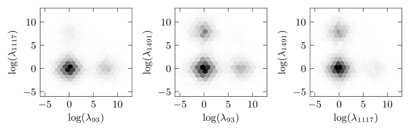
Figure 1: Bivariate density plots from the posterior distribution of the logistic regression model for the Ovarian data. The posterior is 3075-dimensional and is highly multimodal.

1.1 Overview of Importance Sampling

Let us consider an inference problem where a vector of unknown parameters has a probability density function $p(\bm{\theta})$. Our task is to estimate integrals of the form

$$\mu=\mathbb{E}_{p}[h(\bm{\theta})]=\int h(\bm{\theta})p(\bm{\theta})\mathrm{d}\bm{\theta},$$ (1)

where $h(\bm{\theta})$ is some function of the parameters $\bm{\theta}$ that is integrable with respect to $p(\bm{\theta})$. These kinds of integrals are ubiquitous in Bayesian inference, where quantities of interest are computed as expectations over the inferred posterior distribution of the model. However, the same formulation is used for many other problems, such as rare event estimation (Rubino and Tuffin,, 2009), optimal control (Kappen and Ruiz,, 2016), and signal processing (Bugallo et al.,, 2015). Using a set of independent draws $\{\bm{\theta}^{(s)}\}_{s=1}^{S}$ from $p(\bm{\theta})$, the simple Monte Carlo estimator of $\mu$ is

$$\hat{\mu}_{\text{MC}}=\frac{1}{S}\sum_{s=1}^{S}h(\bm{\theta}^{(s)})\,,\,\text{when}\,\,\bm{\theta}^{(s)}\sim p(\bm{\theta}).$$

In this work, we use the term draw to represent a single $\bm{\theta}^{(s)}$, and the term sample to represent a set of draws $\{\bm{\theta}^{(s)}\}_{s=1}^{S}$. If the expectation $\mu$ exists, the simple Monte Carlo estimator is a consistent and unbiased estimator of $\mu$, meaning that asymptotically it will converge towards $\mu$ by the strong law of large numbers. If also the expectation of $h^{2}$ is finite, the central limit theorem holds, and the asymptotic convergence rate of the simple Monte Carlo estimator is proportional to $\mathcal{O}(S^{-1/2})$. Given finite variance, a similar convergence rate holds for uniformly ergodic Markov chains (e.g., Roberts et al.,, 2004).

In some cases, it is not possible or it is expensive to generate draws from $p(\bm{\theta})$, but the expectation $\mu$ is still of interest. In this case, we may generate a sample from a proposal distribution $g(\bm{\theta})$ and compute the expectation of equation (1) using the standard importance sampling estimator

$$\mathbb{E}_{p}[h(\bm{\theta})]\approx\hat{\mu}_{\text{IS}}=\frac{1}{S}\sum_{s=1}^{S}\frac{p(\bm{\theta}^{(s)})}{g(\bm{\theta}^{(s)})}h(\bm{\theta}^{(s)})=\frac{1}{S}\sum_{s=1}^{S}w^{(s)}h(\bm{\theta}^{(s)})\,,\,\text{when}\,\,\bm{\theta}^{(s)}\sim g(\bm{\theta}).$$ (2)

Here, $w^{(s)}$ are called importance weights or importance ratios, and they measure the mismatch between $p(\bm{\theta})$ and $g(\bm{\theta})$ for a specific draw $\bm{\theta}^{(s)}$. In principle, the proposal distribution can be any probability distribution which has the same support as the target distribution $p(\bm{\theta})$ and is positive whenever $p(\bm{\theta})h(\bm{\theta})\neq 0$. The standard importance sampling estimator $\hat{\mu}_{\text{IS}}$ is also a consistent and unbiased estimator of $\mu$ as long as the expectation $\mu$ exists. Its variance depends largely on the choice of the proposal distribution $g(\bm{\theta})$. For a good choice, the variance can be smaller than the variance of the simple Monte Carlo estimator, but it can also be much larger, or infinite, if the choice is less ideal. In the context of this paper, we will consider the simple Monte Carlo estimator simply as a special case of standard importance sampling, where the proposal distribution is $p(\bm{\theta})$, the distribution over which the expectation is defined.

A commonly used alternative estimator is the self-normalized importance sampling (SNIS) estimator

$$\hat{\mu}_{\text{SNIS}}=\frac{\sum_{s=1}^{S}\frac{p(\bm{\theta}^{(s)})}{g(\bm{\theta}^{(s)})}h(\bm{\theta}^{(s)})}{\sum_{s=1}^{S}\frac{p(\bm{\theta}^{(s)})}{g(\bm{\theta}^{(s)})}}=\frac{\sum_{s=1}^{S}w^{(s)}h(\bm{\theta}^{(s)})}{\sum_{s=1}^{S}w^{(s)}}\,,\,\text{when}\,\,\bm{\theta}^{(s)}\sim g(\bm{\theta}).$$ (3)

This estimator is more generally applicable, because it can be used even if the normalization constants of the densities $p(\bm{\theta})$ or $g(\bm{\theta})$ are not known. The self-normalized estimator is also consistent, but has a small bias of order $\mathcal{O}(1/S)$ (Owen,, 2013). All three introduced Monte Carlo estimators are consistent, and thus converge to the true value $\mu$ asymptotically as $S\rightarrow\infty$, if $\mu$ itself exists. However, there are many cases where these estimators can have poor pre-asymptotic behaviour despite having asymptotically guaranteed convergence (Vehtari et al., 2019c, ). That is, in cases with poor pre-asymptotic behaviour, convergence for any achievable finite set of $S$ draws may be so bad, that we cannot get sufficiently accurate results in reasonable time. We discuss this issue in Section 2.3.

To unify the notation and nomenclature of the different Monte Carlo estimators, we define the ratio of the target density $p(\bm{\theta})$ and the proposal density $g(\bm{\theta})$ as the common importance weights because they do not depend on the function $h(\bm{\theta})$ whose expectation is computed:

$$w=w(\bm{\theta})=\frac{p(\bm{\theta})}{g(\bm{\theta})}.$$ (4)

Analogously, we define the product

$$v=v(\bm{\theta})=\frac{p(\bm{\theta})}{g(\bm{\theta})}h(\bm{\theta})$$ (5)

as the expectation-specific importance weights for the expectation $\mathbb{E}_{p}[h(\bm{\theta})]$. With this notation, both the simple Monte Carlo and standard importance sampling estimators are defined as the sample mean of the expectation-specific weights $v$. On the other hand, the self-normalized importance sampling estimator in equation (3) is defined as the ratio of the sample means of $v$ and $w$.

1.2 Multiple Importance Sampling

In this section, we briefly discuss multiple importance sampling, which forms the basis for many existing adaptive importance sampling techniques (Cornuet et al.,, 2012; Martino et al.,, 2015; Bugallo et al.,, 2017). Multiple importance sampling refers to the case of sampling independently from many proposal distributions (Hesterberg,, 1995; Veach and Guibas,, 1995; Owen and Zhou,, 2000). Let us denote the $J$ proposal distributions as $\{g_{1},\ldots,g_{J}\}$ and the number of draws from each as $\{S_{1},\ldots S_{J}\}$ such that $\sum_{j=1}^{J}S_{j}=S$. The multiple importance sampling estimator is a weighted combination of the individual importance sampling estimators:

$$\hat{\mu}_{\text{MIS}}=\sum_{j=1}^{J}\frac{1}{S_{j}}\sum_{s=1}^{S_{j}}\beta_{j}(\bm{\theta}^{(j,s)})\frac{h(\bm{\theta}^{(j,s)})p(\bm{\theta}^{(j,s)})}{g_{j}(\bm{\theta}^{(j,s)})}\,,\,\text{when}\,\,\bm{\theta}^{(j,s)}\sim g_{j}(\bm{\theta}).$$

where $\{\beta_{j}\}_{j=1}^{J}$ is a partition of unity, i.e. for every $\bm{\theta}$, $\beta_{j}(\bm{\theta})\geq 0$ and $\sum_{j=1}^{J}\beta_{j}(\bm{\theta})=1$. With different ways of choosing the weighting functions $\beta_{j}$, one can vary between locally emphasizing one of the proposal distribution $g_{j}$, or considering them in a balanced way for every value of $\bm{\theta}$.

The weighting functions are commonly chosen using a balance heuristic

$$\beta_{j}(\bm{\theta})=\frac{S_{j}g_{j}(\bm{\theta})}{\sum_{k=1}^{J}S_{k}g_{k}(\bm{\theta})},$$

whose variance is proven to be smaller than the variance of any weighting scheme plus a term that goes to zero as the smallest $S_{j}\rightarrow\infty$ (Veach and Guibas,, 1995). The balance heuristic is also a quite natural way of combining the draws from different proposal distributions, as the importance weights for all draws are computed as if they were sampled from the same mixture distribution $g_{\alpha}(\bm{\theta})$

$$w_{\text{DM-MIS}}^{(j,s)}=\frac{p(\bm{\theta}^{(j,s)})}{g_{\alpha}(\bm{\theta}^{(j,s)})}=\frac{p(\bm{\theta}^{(j,s)})}{\sum_{j=1}^{J}\alpha_{j}g_{j}(\bm{\theta}^{(j,s)})},\,\,\,\text{with}\,\,\,\,\alpha_{j}=\frac{S_{j}}{S}.$$ (6)

With these weights, the multiple importance sampling estimator is then computed using the usual equations of standard (eq. (2)) or self-normalized (eq. (3)) importance sampling.

Weights computed using equation (6) are sometimes called deterministic mixture weights, whereas an alternative is to only evaluate a single proposal distribution in the denominator:

$$w_{\text{s-MIS}}^{(j,s)}=\frac{p(\bm{\theta}^{(j,s)})}{g_{j}(\bm{\theta}^{(j,s)})}\,,\,\text{when}\,\,\bm{\theta}^{(j,s)}\sim g_{j}(\bm{\theta}).$$

Deterministic mixture weighting requires more evaluations of the proposal densities, but the variance of the resulting estimator is lower (Elvira et al.,, 2019) There are techniques for improving the efficiency of the balance heuristic (Havran and Sbert,, 2014; Elvira et al.,, 2015, 2016; Sbert et al.,, 2016; Sbert and Havran,, 2017; Sbert and Elvira,, 2019). In this work, we use the balance heuristic because of its simplicity and empirically shown good performance.

1.3 Adaptive Importance Sampling

Adaptive importance sampling is a general term that refers to an iterative process for updating a single or multiple proposal distributions to approximate a given target distribution. The details of the adaptation can vary in multiple ways, but most methods consist of three steps: i) generating draws from the proposal distribution(s), ii) computing the importance weights of the draws, and iii) adapting the proposal distribution(s).

Adaptive importance sampling methods can be categorized in multiple ways, for example based on the type and number of proposal distributions, weighting scheme, and adaptation strategy. Most methods use one or more parametric proposal distributions, such as Gaussian or Student-$t$ distributions. Typical adaptation strategies are resampling or moment estimation based on the importance weights. A good review of many different methods and their classification is presented in Bugallo et al., (2017). For discussion about the convergence of adaptive importance sampling methods, see, for example, Feng et al., (2018) and Akyildiz and Míguez, (2019).

Some notable recent algorithms are adaptive multiple importance sampling (AMIS; Cornuet et al.,, 2012) and adaptive population importance sampling (APIS; Martino et al.,, 2015), which both use multiple proposal distributions, and weighting based on deterministic mixture weights. For the adaptation, they rely on weighted moment estimation to adapt the mean (and possibly covariance) of the proposal distributions. Population Monte Carlo algorithms are another class of adaptive importance sampling methods, which typically use weighted resampling as the means of adaptation (Cappé et al.,, 2004, 2008; Elvira et al.,, 2017).

2 Importance Weighted Moment Matching

In this section, we present our proposed implicit adaptive importance sampling method, importance weighted moment matching (IWMM). We start from the assumption that we have a Monte Carlo sample and we are computing an expectation of some function as in equation (1). The sample can be from an arbitrary importance sampling proposal distribution, or it can be from the actual distribution over which the expectation is defined. As with any adaptive importance sampling method, our motivation is that the accuracy of the expectation using the current sample is not good enough. The situation where the proposed framework is most beneficial is when the sample is from a relatively good, complex proposal distribution with no closed form and which is expensive to sample from. Situations like this arise often in Bayesian inference, when a Monte Carlo sample from the full data posterior distribution has been sampled, and model evaluations using cross-validation or bootstrap are of interest (Gelfand et al.,, 1992; Gelfand,, 1996; Peruggia,, 1997; Epifani et al.,, 2008; Vehtari et al.,, 2017; Giordano et al.,, 2019). In this case, implicit adaptation of the proposal distribution can benefit from the existing sample and improve Monte Carlo accuracy with a small computational cost.

There are similar approaches that adapt proposal distributions nonparametrically using e.g. kernel density estimates (Zhang,, 1996). With the implicit adaptation, we avoid both the resampling and density estimation steps. Unbiased path sampling by Rischard et al., (2018) can also use arbitrary proposal distributions, but their approach requires a considerable amount of tuning from the user.

2.1 Target of Adaptation

Let us recap the three general steps of adaptive importance sampling, which are i) generating draws from the proposal distribution(s), ii) computing the importance weights of the draws, and iii) adapting the proposal distribution(s) based on the weights. In our proposed method, step i) is omitted because we do not resample during adaptation, and instead use the same sample that is transformed directly. For this reason, the method can be used with any Monte Carlo sample whose probability density function is known.

For step ii), unlike most adaptive importance sampling methods, we are not primarily interested in perfectly adapting the proposal distribution to the distribution over which the expectation is defined, which is often called the target distribution in the importance sampling literature. While this is a reasonable goal in many cases, in sections 3.1 and 3.2 we show examples where sampling from the target distribution itself leads to extremely biased estimates. Instead, we are mainly interested in adapting to the theoretical optimal proposal distribution of a given expectation $\mathbb{E}_{p}[h(\bm{\theta})]$, which depends on three things: the distribution $p(\bm{\theta})$ over which the expectation is defined, the function $h(\bm{\theta})$ whose expectation is computed, and the Monte Carlo estimator that is used. For the standard importance sampling estimator, the optimal proposal distribution is proportional to (Kahn and Marshall,, 1953)

$$g_{\text{IS}}^{\text{opt}} (\bm{\theta})\propto p(\bm{\theta})\,|h(\bm{\theta})\,|,$$ (7)

and for the self-normalized importance sampling estimator, it is (Hesterberg,, 1988)

$$g_{\text{SNIS}}^{\text{opt}} (\bm{\theta})\propto p(\bm{\theta})\,|h(\bm{\theta})-\mathbb{E}_{p}[h(\bm{\theta})]\,|.$$ (8)

The more complicated form for the self-normalized estimator is due to the requirement of accurate estimation of both the numerator and denominator of equation (3) simultaneously.

In order to approach the optimal proposal distribution, we define the importance weights for adaptation as follows: When using the standard importance sampling (or simple Monte Carlo) estimator, we use the absolute values of the expectation-specific weights of equation (5) for adaptation, because they quantify the mismatch between the current proposal and the optimal proposal density. For the self-normalized importance sampling estimator, we recommend separate adaptations for the numerator and the denominator, using the absolute values of the expectation-specific weights and the common importance weights, respectively. The results of the two adaptations are combined with multiple importance sampling to approximate the optimal proposal density of equation (8). To combine the two adaptations into an efficient proposal distribution, we use an approximation based on superimposing a simpler distribution on top of the optimal proposal:

$$g_{\text{SNIS}}^{\text{split}}(\bm{\theta})\propto|h(\bm{\theta})|p(\bm{\theta})+\mathbb{E}_{p}[h(\bm{\theta})]p(\bm{\theta}).$$ (9)

We call this the split proposal density, because it splits the piecewise defined density of equation (8) into two clear components. The first component is proportional to equation (7) and is thus approximated with the adaptation using the absolute expectation-specific weights. The second component is proportional to $p(\bm{\theta})$ and is reached with the adaptation using the common weights.

Equation (9) is a convenient approximation to the optimal proposal of self-normalized importance sampling because it has similar tails while being simpler to sample from because it has two clear components, whereas the density in equation (8) can easily be multimodal even when the expectation is defined over a unimodal distribution. The drawback of this approximation is that it places unnecessary probability mass in areas where $h(\bm{\theta})\approx\mathbb{E}_{p}[h(\bm{\theta})]$, thus losing some efficiency. However, generally the more distinct $p(\bm{\theta})$ is from $p(\bm{\theta})|h(\bm{\theta})|$, the smaller $\mathbb{E}_{p}[h(\bm{\theta})]$ becomes and hence the approximation becomes closer to the optimal form. Fortunately, these are the cases when adaptive importance sampling techniques are most needed. In Figure 4 in Appendix C.1, we show an example of this phenomenon.

Because equation (9) is a sum of two terms, it is essentially a multiple importance sampling proposal distribution with two components. The number of Monte Carlo draws that should be allocated to each component depends on the properties of $p(\bm{\theta})$ and $h(\bm{\theta})$. A conservative choice is to allocate the same number to both terms. When $h(\bm{\theta})$ is nonnegative, this is actually the optimal allocation, because both terms in equation (9) integrate to $\mathbb{E}_{p}[h(\bm{\theta})]$. With this allocation, multiple sampling with the balance heuristic is safe in the sense that the asymptotic variance of the estimator is never larger than $2$ times the variance of standard importance sampling using the better component (He and Owen,, 2014). We note that the double adaptation and combining with equation (9) is possible and beneficial also with existing parametric adaptive importance sampling methods. We demonstrate this in the experiments section.

2.2 Affine Transformations

Step iii) of adaptive importance sampling is the adaptation of the current proposal distribution(s). Two commonly used adaptation techniques are weighted resampling and moment estimation (Bugallo et al.,, 2017). In parametric adaptive importance sampling methods, weighted moment estimation is used to update the location and scale parameters of the parametric proposal distribution. We employ a similar idea, but instead directly transform the Monte Carlo sample using an affine transformation. This enables adaptation of proposal distributions which do not have a location-scale parameterisation or even a closed form representation. The only requirement is that the (possibly unnormalized) probability density is computable. This property makes it useful in many practical situations where a Monte Carlo sample has been generated with probabilistic programming tools, or other Markov chain Monte Carlo methods. By using a reversible transformation, we can compute the probability density function of the transformed draws in the adapted proposal with the Jacobian of the transformation.

In this work, we consider simple affine transformations, because both the transformation and its Jacobian are computationally cheap. Consider approximating the expectation $\mathbb{E}_{p}[h(\bm{\theta})]$ with a set of draws $\{\bm{\theta}^{(s)}\}_{s=1}^{S}$ from an arbitrary proposal distribution $g(\bm{\theta})$ (which can also be $p(\bm{\theta})$ itself). For a specific draw $\bm{\theta}^{(s)}$, a generic affine transformation includes a square matrix $\mathbf{A}$ representing a linear map, and translation vector $\mathbf{b}$:

$$T:\bm{\theta}^{(s)}\mapsto\mathbf{A}\bm{\theta}^{(s)}+\mathbf{b}=:\accentset{\ast}{\bm{\theta}}^{(s)}.$$ (10)

Because the transformation is affine and the same for all draws, the new implicit density $g_{T}$ evaluated at every $\accentset{\ast}{\bm{\theta}}^{(s)}$ changes by a constant, namely the inverse of the determinant of the Jacobian, $|\mathbf{J}_{T}|^{-1}=\left|\frac{\mathrm{d}T(\bm{\theta})}{\mathrm{d}\bm{\theta}}\right|^{-1}$. Note that to compute the inverse, the matrix $\mathbf{A}$ must be invertible. After the transformation, the implicit probability density of the adapted proposal $g_{T}$ for the transformed draw $\accentset{\ast}{\bm{\theta}}^{(s)}$ is

$$g_{T}(\accentset{\ast}{\bm{\theta}}^{(s)})=g(\bm{\theta}^{(s)})|\mathbf{J}_{T}|^{-1}.$$

If the original proposal density $g$ was known only up to an unknown normalizing constant, the adapted proposal $g_{T}$ has that same unknown constant. This is crucial in order to be able to use the split proposal distribution of equation (9) for self-normalized importance sampling.

To reduce the mismatch between a Monte Carlo sample $\{\bm{\theta}^{(s)}\}_{s=1}^{S}$ and a given adaptation target, we consider three affine moment matching transformations with varying degrees of simplicity. The transformation have a similar idea as warp transformations used for bridge sampling by Meng and Schilling, (2002). The importance weights used in the transformations can be either the common weights or the expectation-specific weights, depending on what the adaptation target is, as discussed in Section 2.1. We define the first transformation, $T_{1}$, to match the mean of the sample to its importance weighted mean:

$$\accentset{\ast}{\bm{\theta}}^{(s)} =T_{1}(\bm{\theta}^{(s)})=\bm{\theta}^{(s)}-\overline{\bm{\theta}}+\overline{\bm{\theta}}_{w},$$

$$\overline{\bm{\theta}} =\frac{1}{S}\sum_{s=1}^{S}\bm{\theta}^{(s)},$$

$$\overline{\bm{\theta}}_{w} =\frac{\sum_{s=1}^{S}w^{(s)}\bm{\theta}^{(s)}}{\sum_{s=1}^{S}w^{(s)}}.$$

We define $T_{2}$ to match the marginal variance in addition to the mean:

$$\accentset{\ast}{\bm{\theta}}^{(s)} =T_{2}(\bm{\theta}^{(s)})=\mathbf{v}_{w}^{1/2}\circ\mathbf{v}^{-1/2}\circ(\bm{\theta}^{(s)}-\overline{\bm{\theta}})+\overline{\bm{\theta}}_{w},$$

$$\mathbf{v} =\frac{1}{S}\sum_{s=1}^{S}(\bm{\theta}^{(s)}-\overline{\bm{\theta}})\circ(\bm{\theta}^{(s)}-\overline{\bm{\theta}}),$$

$$\mathbf{v}_{w} =\frac{\sum_{s=1}^{S}w^{(s)}(\bm{\theta}^{(s)}-\overline{\bm{\theta}})\circ(\bm{\theta}^{(s)}-\overline{\bm{\theta}})}{\sum_{s=1}^{S}w^{(s)}},$$

where $\circ$ refers to a pointwise product of the elements of two vectors. The final transformation, $T_{3}$, matches the covariance and the mean:

$$\accentset{\ast}{\bm{\theta}}^{(s)} =T_{3}(\bm{\theta}^{(s)})=\mathbf{L}_{w}\mathbf{L}^{-1}(\bm{\theta}^{(s)}-\overline{\bm{\theta}})+\overline{\bm{\theta}}_{w},$$

$$\mathbf{L}\mathbf{L}^{\mathsf{T}} =\bm{\Sigma}=\frac{1}{S}\sum_{s=1}^{S}(\bm{\theta}^{(s)}-\overline{\bm{\theta}})(\bm{\theta}^{(s)}-\overline{\bm{\theta}})^{\mathsf{T}},$$

$$\mathbf{L}_{w}\mathbf{L}_{w}^{\mathsf{T}} =\bm{\Sigma}_{w}=\frac{\sum_{s=1}^{S}w^{(s)}(\bm{\theta}^{(s)}-\overline{\bm{\theta}}_{w})(\bm{\theta}^{(s)}-\overline{\bm{\theta}}_{w})^{\mathsf{T}}}{\sum_{s=1}^{S}w^{(s)}}.$$

If the weights are available with the correct normalization, the weighted moments can be computed using standard importance sampling, but for a more general case, we show the self-normalized estimators of the weighted moments. When relying on self-normalized importance sampling, we recommend two separate adaptations, as discussed in Section 2.1. We perform both adaptations separately with the full Monte Carlo sample, but for the multiple importance sampling estimator of equation (9) we split the existing sample into two equally sized parts to avoid causing bias from using the same draws twice.

The three affine transformations are defined from simple to complex in terms of the effective sample size required to accurately compute the moments (Kong,, 1992; Martino et al.,, 2017; Chatterjee et al.,, 2018; Elvira et al.,, 2018). Especially in the third transformation, the weighted covariance can be impossible to compute if the variance of the weight distribution is large. For this reason, we first iterate only $T_{1}$ repeatedly, and move on to $T_{2}$ and $T_{3}$ only when $T_{1}$ is no longer helping. To determine this, we use finite sample diagnostics which will be discussed next.

2.3 Stopping Criteria and Diagnostics

Even if an (adaptive) importance sampling procedure has good asymptotic properties or the used proposal distribution guarantees finite variance by construction, its pre-asymptotic behaviour can be poor. Because of this, finite sample diagnostics are extremely important for assessing pre-asymptotic behaviour. For example, Vehtari et al., 2019c demonstrate importance sampling cases with asymptotically finite variance, but pre-asymptotic behavior indistinguishable from cases with unbounded importance weights or infinite variance. Vehtari et al., 2019c propose a finite sample diagnostic based on fitting a generalized Pareto distribution to the upper tail of the distribution of the importance weights. Because theoretically the shape parameter $k$ of the generalized Pareto distribution determines the number of its finite moments, the fitted distribution and its shape parameter $\hat{k}$ are useful for estimating practical pre-asymptotic convergence rate. The authors propose $\hat{k}=0.7$ as an upper limit of practically useful pre-asymptotic convergence. The stability of (self-normalised) importance sampling can be improved by replacing the largest weights with ordered statistics of the generalized Pareto distribution estimated already for the diagnostic purposes.

The Pareto $\hat{k}$ diagnostic can also be used as a stopping criterion for adaptive importance sampling methods in order to not run the adaptation excessively long and waste computational resources. In addition to that, in the importance weighted moment matching method we use the diagnostic for estimating whether a specific transformation improves the proposal distribution or not.

We use the Pareto diagnostic as follows. First, we compute the Pareto $\hat{k}$ diagnostic value for the original (common or expectation-specific) weights. After a transformation ($T_{1}$, $T_{2}$ or $T_{3}$) we recompute the diagnostic, and only accept the transformation if the diagnostic value has decreased. If it has, the transformation is accepted and the weights and diagnostic value are updated. We begin the adaptation by repeating transformation $T_{1}$, and only when it is no longer accepted, we move on to attempt transformation $T_{2}$, and eventually $T_{3}$. As a criterion for stopping the whole algorithm, we use the diagnostic value $\hat{k}=0.7$ as recommended by Vehtari et al., 2019c as a practical upper limit for useful accuracy.

The full importance weighted moment matching algorithm for standard importance sampling or simple Monte Carlo sampling is presented in Algorithm 1. When using self-normalized importance sampling, the algorithm is very similar, with the exception of having two separate adaptations and combining them with multiple importance sampling in the end. It is presented as Algorithm 2 in Appendix A.

Algorithm 1 Moment matching for standard importance sampling

1:  Input: $k_{\text{threshold}}$, proposal density $g$, draws $\{\bm{\theta}_{i}^{(s)}\}_{s=1}^{S}$ from $g$

2:  Compute expectation-specific weights $\{v^{(s)}\}_{s=1}^{S}$ and compute diagnostic $\hat{k}$;

3:  while $\hat{k}>k_{\text{threshold}}$ do

4:     for $j$ in $1:3$ do

5:        Transform the draws with $T_{j}:\bm{\theta}^{(s)}\mapsto\accentset{\ast}{\bm{\theta}}^{(s)}$ using absolute expectation-specific weights;

6:        Recompute expectation-specific weights $\{\accentset{\ast}{v}^{(s)}\}_{s=1}^{S}$ and $\hat{\accentset{\ast}{k}}$;

7:        if $\hat{\accentset{\ast}{k}}<\hat{k}$ then

8:           Accept the transformation and update $\{\bm{\theta}^{(s)}\}_{s=1}^{S}=\{\accentset{\ast}{\bm{\theta}}^{(s)}\}_{s=1}^{S}$, $\{v^{(s)}\}_{s=1}^{S}=\{\accentset{\ast}{v}^{(s)}\}_{s=1}^{S}$, and $\hat{k}=\hat{\accentset{\ast}{k}}$;

9:           Exit for loop;

10:        else

11:           Discard the transformation;

12:        end if

13:        if $j==3$ then

14:           Moment matching failed because $\hat{k}>k_{\text{threshold}}$, end algorithm with a warning about sampling inaccuracy;

15:        end if

16:     end for

17:  end while

18:  Moment matching succeeded, compute expectation $\mathbb{E}_{p}[h(\bm{\theta})]$ using equation (2);

2.4 Computational Cost

The computational cost of several popular adaptive importance sampling methods are compared in Table 1. We show here the methods which also use moment estimation and are thus most similar to the proposed importance weighted moment matching method. For a more exhaustive comparison, see the review paper by Bugallo et al., (2017). Because of the implicit adaptation in IWMM, the proposal density needs to be computed only once at the beginning of the algorithm. Thus, the computational complexity of IWMM is smaller than even the simplest single-proposal adaptive importance sampling methods. It is thus well suited for problems where target evaluations are expensive. We note that IWMM could also replicate the proposal distribution of consecutive transformations in a similar fashion as adaptive multiple importance sampling to increase performance at the cost of increased computational complexity (Cornuet et al.,, 2012). However, this may cause bias because there is no resampling. We leave this as possible direction for future research.

Table 1: Total computational costs of different adaptive importance sampling algorithms after $T$ iterations. $S$ represents the number of draws sampled per iteration from each proposal distribution, except for IWMM which does not resample. $N$ represents the number of proposal distributions.

Algorithm	Target evaluations	Proposal evaluations
importance weighted
moment matching (IWMM)	$\mathcal{O}(ST)$	$\mathcal{O}(S)$
single-proposal adaptive
importance sampling (AIS)	$\mathcal{O}(ST)$	$\mathcal{O}(ST)$
adaptive multiple
importance sampling (AMIS)	$\mathcal{O}(ST)$	$\mathcal{O}(ST^{2})$
adaptive population
importance sampling (APIS)	$\mathcal{O}(NST)$	$\mathcal{O}(N^{2}ST)$

If the importance weights have large variance, the moment matching transformations can be noisy because of inaccurate computation of the weighted moments. There are two principal ways to remediate this. First, increasing the number of draws generally increases the accuracy of the computed moments. Second, the importance weights used for computing the weighted moments can be regularized with truncation or smoothing methods (Ionides,, 2008; Koblents and Míguez,, 2015; Miguez et al.,, 2018; Vehtari et al., 2019c, ; Bugallo et al.,, 2017). In the experiments section, we demonstrate that the accuracy of the moment matching can be improved with Pareto smoothing from Vehtari et al., 2019c .

Another shortcoming of the method is that the adaptation target is not always well characterized by its first and second moments, and the target and proposal distributions can differ in several characteristics, such as tail thickness, correlation structure, or number of modes. For complex targets, more elaborate transformations may be needed to reach a good enough proposal distribution. That being said, it is not necessary to match all characteristics of the proposal distribution to the target for importance sampling to be effective.

3 Experiments

In this section, the proposed implicit adaptation method is illustrated with a variety of numerical experiments using leave-one-out cross-validation (LOO-CV) as an example application. With both simulated and real data sets, we evaluate the predictive performance of different Bayesian models using leave-one-out cross-validation, and demonstrate the improvements that the implicit adaptation methods can provide. We also compare it to existing adaptive importance sampling methods that use parametric proposal distributions.

All of the simulations were done in R (R Core Team,, 2020), and the models were fitted using rstan, the R interface to the Bayesian inference package Stan (Carpenter et al.,, 2017; Stan Development Team,, 2018). To sample from the posterior of each model, we ran four Markov chains using a dynamic Hamiltonian Monte Carlo (HMC) algorithm (Hoffman and Gelman,, 2014; Betancourt,, 2017) which is the default in Stan. We monitor convergence of the chains with the split-$\widehat{R}$ potential scale reduction factor from Vehtari et al., 2019b and by checking for divergence transitions, which is a diagnostic specific to adaptive HMC. We note that the finite sample behaviour of Monte Carlo integrals depends on the algorithm used to generate the sample. For example, if one uses an MCMC algorithm less efficient than HMC, the resulting Monte Carlo approximations will generally be worse than those illustrated in the next sections. R and Stan codes of the experiments and the used data sets are available on Github (https://github.com/topipa/iter-mm-paper).

Because probabilistic programming tools generally give only unnormalized posterior densities, we mostly focus on self-normalized importance sampling. As the default case, we take the situation that Monte Carlo draws are available from the full data posterior distribution, and these are adapted using our proposed method. We note that leave-one-out cross-validation in this setting is a special case such that the double adaptation which is discussed in Section 2.1 is not needed even when using self-normalized importance sampling. The split proposal of equation (9) is still used, but the other term uses the full data posterior draws. To help the reader in understanding or implementing the methods, we have presented the basics of Bayesian leave-one-out cross-validation as well as instructions for implementing the proposed methods in Appendix B. In addition to importance sampling, we also discuss simple Monte Carlo sampling results when sampling from each leave-one-out posterior explicitly.

By default, we use Pareto smoothing to stabilize importance weights, but we also present results without smoothing (Vehtari et al.,, 2017; Vehtari et al., 2019c, ). This enables us to also monitor the reliability of the Monte Carlo estimates using the Pareto $\hat{k}$ diagnostics. We show that the diagnostics accurately identify convergence problems in not only importance sampling, but also when using the simple Monte Carlo estimator or adaptive importance sampling algorithms. Based on Vehtari et al., 2019c , we use $\hat{k}=0.7$ as an upper threshold to indicate practically useful finite sample convergence rate.

We compare our proposed method to several existing adaptive importance sampling methods. For comparison, we chose algorithms that are conceptually similar to our proposed implicit adaptation method. As the first comparison, we have generic adaptive importance sampling methods, which use a single proposal distribution and adapt the location and scale parameters of this distribution using weighted moment estimation. As the proposal distribution we have either a multivariate Gaussian distribution, or a Student-$t_{3}$ distribution. Moreover, we test these algorithms in the traditional way of adapting using the common importance weights, and also using our proposed double adaptation, resulting in 4 different algorithms. To compare to a more powerful and computationally expensive algorithm, we chose adaptive multiple importance sampling (AMIS; Cornuet et al.,, 2012), which uses multiple proposal distributions and deterministic mixture weighting, increasing the number of proposal distributions over time. Also for this algorithm, we test 4 versions by having either Gaussian or Student-$t_{3}$ distributions as well as with and without double adaptation. We start all the parametric adaptive methods with mean and covariance estimated from a sample from the full data posterior. Also for the parametric adaptive importance sampling methods, we use the Pareto $\hat{k}$ diagnostic to determine when to stop the algorithm. For all eight algorithms, we adapt both the mean and covariance if it is feasible, but for very high-dimensional distributions we only adapt the mean, because otherwise the adaptation is unstable given the used sample sizes.

Sections 3.1 and 3.2 show low-dimensional examples where the function $h$ whose expectation is being computed gets large values in the tails of the distribution over which the expectation is being computed. These cases highlight the importance of our proposed double adaptation, as the target densities are available in unnormalized form. Sections 3.3 and 3.4 show correlated and high-dimensional examples which are significantly more difficult. In Section 3.4, the distribution over which the expectation is defined is also multimodal. In these cases, we demonstrate the usefulness of using a complex non-parametric proposal distribution instead of Gaussian or Student-$t$ densities.

3.1 Experiment 1: Gaussian Data with a Single Outlier

In this section, we demonstrate with a simple example what happens when we try to assess the predictive performance of a misspecified model. We emphasize that even though this is a simple example, it still provides valuable insight for real world data and models as evaluating misspecified models is an integral part of any Bayesian modelling process. In terms of Monte Carlo sampling, this is an example of an expectation (1) where the largest values of the function $h$ are in the tails of the target distribution $p$.

We generate 29 observations from a standard normal distribution, and manually set the value for a 30’th observation to introduce an outlier. This mimics a situation where the true data generating mechanism has thicker tails than the assumed observation model. Keeping the randomly generated observations fixed, we repeat the experiment for different values of the outlier ranging from $y_{30}=0$ to $y_{30}=20$. We model the data with a Gaussian distribution with unknown mean and variance, generate draws from the model posterior, and evaluate the predictive ability of the model using leave-one-out cross-validation.

For all 30 observations, represented jointly by the vector $\mathbf{y}$, the model is thus

$$\mathbf{y}\sim\text{Normal}(\mu,\sigma^{2})$$

with mean $\mu$ and standard deviation $\sigma$. We set improper uniform priors on $\mu$ and $\log(\sigma)$. In this model, the posterior predictive distribution $p(\widetilde{y}\mid\mathbf{y})$ is known analytically, and is a Student $t$-distribution with $n-1$ degrees of freedom, mean at the mean of the data, and scale $\sqrt{1+1/n}$ times the standard deviation of the data, where $n$ is the number of observations. Thus, we can compute the Bayesian LOO-CV estimate for the single left out point analytically via

$$\text{elpd}_{\text{loo},i}=\log p(\widetilde{y}=y_{i}\mid\mathbf{y}_{-i}).$$

The left plot of Figure 2 shows the computed $\widehat{\text{elpd}}_{\text{loo},30}$ estimates for the $30$’th observation based on different sampling methods, which are compared to the analytical $\text{elpd}_{\text{loo},30}$ values when the outlier value is varied. When the outlier becomes more and more different from the rest of the observations and the analytical $\text{elpd}_{\text{loo},30}$ decreases, both the simple Monte Carlo estimate from the true leave-one-out posterior and the PSIS estimate from the full data posterior become more and more biased due to insufficient accuracy in the tails of the posterior predictive distribution. The same happens to adaptive importance sampling using a single Gaussian proposal (AIS-G), and to a smaller extent when using a Student-$t_{3}$ proposal (AIS-$t$). Our proposed importance weighted moment matching from either the full posterior (PSIS+MM) or the leave-one-out posterior (naive+MM) almost perfectly align with the analytical solution. Also the AIS-G and AIS-$t$ give very accurate results when using our proposed double adaptation. Similarly, the results of all 4 AMIS algorithms align well with the analytical solution and are omitted in Figure 2 for improved readability. While not shown in the plot, also PSIS+MM gives highly biased results if omitting the split proposal of equation (9). In Appendix C, we show the results of a similar experiment, where the randomly generated points $y_{1}$ to $y_{29}$ are re-generated at every repetition to show that the results are not just specific to this particular data realization.

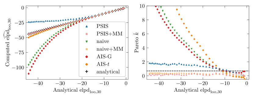
Figure 2: Computed $\widehat{\text{elpd}}_{\text{loo},30}$ estimates of the left out observation $y_{30}$ for the normal model for different values between $y_{30}=0$ and $y_{30}=20$. The black crosses depict the analytical results. The sampling results are averaged from 100 independent Stan runs, and the error bars represent $95\%$ intervals of the mean across these runs. The dashed line at $\hat{k}=0.7$ presents the diagnostic threshold indicating practically useful finite sample convergence rate.

The right plot of Figure 2 shows the Pareto $\hat{k}$ diagnostic values corresponding to the different algorithms. The diagnostic values are computed from both common and expectation-specific weights, and the larger is reported. The plot shows that both moment matching algorithms have $\hat{k}<0.7$ which indicates good finite sample accuracy. For all of the other algorithms, the diagnostic value grows over 0.7 when the problem becomes more difficult, which correlates well with the biased results in the left plot. From the AIS algorithms, the Student-$t_{3}$ proposal distribution has much smaller bias compared to the Gaussian proposal due to its much thicker tails. Still, the Pareto $\hat{k}$ diagnostic indicates poor finite sample convergence. When looking at the importance weights of the individual runs, it is indeed clear that the result is based on only a few Monte Carlo draws from the thick tails of the Student-$t_{3}$ distribution. Because of that, the variance between different runs is large. In the most difficult case when $y_{30}=20$ and $\text{elpd}_{\text{loo},30}=-44.3$, the variance of the estimated $\text{elpd}_{\text{loo},30}$ for $\text{AIS-}t$ is more than 1000 times higher than for PSIS+MM.

Figure 2 highlights the importance of our proposed double adaptation when some densities are available in unnormalized form. All of the proposal distributions that we compared fail without the double adaptation and split proposal of equation (9). The Student-$t$ proposal does quite well, but it has high variance because of relying only on a few draws from the tails. In more high-dimensional situations, it will also fail quicker, as we show later. AMIS gives good results even without the double adaptation because it was started from an initial distribution based on the mean and covariance of the full posterior, and it retains all earlier proposal distributions. Because this is already close to the target of the second adaptation, it is not needed for the AMIS algorithms in this low-dimensional example.

3.2 Experiment 2: Poisson Regression with Outliers

In the second experiment, we illustrate with a real data set how poor finite sample convergence can cause significant errors when estimating predictive performance of models. The data are from Gelman and Hill, (2006), where the authors describe an experiment that was performed to assess how efficiently a pest management system reduces the amount of roaches. The target variable $y$ describes the number of roaches caught in a set of traps in each apartment. The model includes an intercept plus three regression predictors: the number of roaches before treatment, an indicator variable for the treatment or control group, and an indicator variable for whether the building is restricted to elderly residents. We will fit a Poisson regression model with a log-link to the data set. The traps were held in the apartments for different periods of time, so the measurement time is included by adding its logarithm as an offset to the linear predictor. The model has only 4 parameters, so this is again a quite simple example.

On the left side of Figure 3 we show the computed $\widehat{\mathrm{elpd}}_{\mathrm{loo}}$ estimates averaged from 100 independent Stan runs as a function of the number of posterior draws $S$. On the right side, the mean of the largest Pareto $\hat{k}$ diagnostic values out of all of the observations are presented. The diagnostic is always computed from both the common and expectation-specific weights, and the larger is reported. There is a large difference between the PSIS and naive estimates, and they approach each other very slowly when increasing $S$, which is due to the poor convergence rate, as indicated by the high Pareto $\hat{k}$ values on the right side plot. Importance weighted moment matching from either the full posterior or leave-one-out posteriors gives reliable estimates with very small error already from 1000 draws. The accuracy is confirmed by the changed Pareto $\hat{k}$ values which are always below 0.7. For the single-proposal parametric methods, using the Student-$t_{3}$ proposal distributions and doing our proposed double adaptation (AIS-$t$ $\times 2$) gives good results from 2000 draws onwards, but the rest of the methods give highly biased results even with $S=64000$. Contrary to the previous example, now even the double adaptation converges extremely slowly when using a Gaussian proposal distribution (AIS-G $\times 2$), which indicates that the posterior distribution is non-Gaussian. All 4 versions of the AMIS algorithms had Pareto $\hat{k}$ values below 0.7 already with 1000 draws, and had elpd estimates almost indistinguishable from the importance weighted moment matching results. These are omitted from Figure 3 for improved readability.

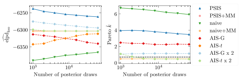
Figure 3: Left: Computed $\widehat{\mathrm{elpd}}_{\mathrm{loo}}$ estimates over the whole Roach data set as a function of the number of posterior draws $S$. Right: The mean of the largest Pareto $\hat{k}$ diagnostic values among the observations. The results are averaged from 100 independent Stan runs, and the error bars represent $95\%$ intervals of the mean across these runs. The dashed line at $\hat{k}=0.7$ presents the diagnostic threshold indicating practically useful finite sample convergence rate. The largest Pareto $\hat{k}$ for AIS-$t$ is around 10, and it is left out of the right plot for clarity.

3.3 Experiment 3: Linear Regression with Correlated Predictor Variables

In the previous examples, the used models were quite simple and had a small number of parameters. In this and the following sections, we study the limitations of the importance weighted moment matching method by considering models with more parameters and correlated or non-Gaussian posteriors. The two previous experiments showed that the Pareto $\hat{k}$ diagnostic is a reliable indicator of finite sample accuracy for adaptive importance sampling methods. To demonstrate the performance and computational cost of the different adaptive algorithms, we report the number of leave-one-out (LOO) folds where the algorithms fail to decrease the $\hat{k}$ diagnostic value below $0.7$. In order to get reliable results for these failed LOO folds, the user should generate new MCMC draws from the LOO posterior, which can be very costly. We fit all models to the full data set, and report the number of leave-one-out folds where the $\hat{k}$ diagnostic value is above $0.7$ when using the full data posterior directly as a proposal distribution. These are reported in the column PSIS in Table 2. We run the moment matching algorithm for all these LOO folds, and report how many $\hat{k}$ values are still above $0.7$ (PSIS+MM). Similarly, we run the 8 parametric adaptive methods for the same LOO folds. In Table 2, we only show the best performing parametric methods, which are AMIS with double adaptation using either Gaussian or Student-$t_{3}$ proposals (AMIS $\times 2$ and AMIS-$t$ $\times 2$). In the lower part of Table 2, we report run times in seconds for all the reported algorithms. The run times are based on single core runs with an Intel Xeon X5650 2.67 GHz processor.

For this experiment, we simulated data from a linear regression model. The data consists of $n=60$ observations of one outcome variable and $30$ predictors that are correlated with each other by correlation coefficient of $\rho=0.8$. Three of the true regression coefficients are nonzero, and the rest are all zero. Independent Gaussian noise was added to the outcomes $\mathbf{y}$. Because the predictors are strongly correlated, importance sampling leave-one-out cross-validation is difficult and we get multiple high Pareto $\hat{k}$ values when using the full data posterior as the proposal distribution. The results of Table 2 show that already with 2000 posterior draws, the moment matching algorithm is able to decrease the Pareto $\hat{k}$ values of all LOO folds below $0.7$. In contrast, none of the parametric algorithms ever succeed in reducing $\hat{k}$ values below $0.7$, even when increasing the number of draws to 8000. This highlights the difficulty of adapting to a highly correlated distribution. Because the moment matching starts from the full data posterior sample, which is similarly correlated, the moment matching can successfully improve the proposal distribution with a small cost. The AMIS algorithms were run for 10 iterations to limit the computational cost. By increasing the number of iterations, they should succeed eventually, but at a high computational cost. In Table 3 in Appendix C, we show results for importance weighted moment matching without Pareto smoothing the importance weights. The results are slightly worse compared to the Pareto smoothing case.

3.4 Experiment 4: Binary Classification in a Small $n$ Large $p$ Data Set

In the fourth experiment, we have a real microarray Ovarian cancer classification data set with a large number of predictors and small number of observations. The data set has been used as a benchmark by several authors (e.g. Schummer et al.,, 1999; Hernández-Lobato et al.,, 2010, and references). The data consists of $54$ measurements and has $1536$ predictor variables. We will fit a logistic regression model using a regularized horseshoe prior (Piironen and Vehtari, 2017b, ) on the regression coefficients because we expect many of them to be zero. This data set and model are difficult for several reasons. First, because the amount of observations is quite low, leaving out single observations changes the posterior significantly, indicated by a large number of high Pareto $\hat{k}$ values. Second, because the number of parameters in the model is 3075, moment matching in the high-dimensional space is difficult. Third, the posterior distribution of several parameters is multimodal, as illustrated in Figure 1. Because of the multimodality, we used Monte Carlo chains of length 1000, and increased the number of chains when increasing $S$.

When fitting the model to the full data posterior, Table 2 shows the number of LOO folds with $\hat{k}>0.7$ before and after moment matching. The results show that already with 1000 draws, PSIS+MM is able to reduce $\hat{k}$ of many LOO folds below 0.7. Investing more computational resources by collecting more posterior draws increases the moment matching accuracy, and more LOO folds can be improved. However, even with $8000$ posterior draws some folds have $\hat{k}>0.7$ after moment matching, and thus the $\widehat{\text{elpd}}_{\text{loo}}$ estimate may not be reliable. Again, none of the parametric adaptive methods succeed in reducing Pareto $\hat{k}$ values below 0.7 in 10 iterations. The lower part of Table 2 also shows the significantly higher computational time of the AMIS algorithms compared to importance weighted moment matching.

Table 2: Upper part: Numbers of LOO folds with Pareto $\hat{k}$ diagnostic above 0.7 when the models are fitted to the full data set (lower is better). Lower part: Average run times in seconds for different algorithms. Column PSIS corresponds to using the full data posterior directly as the proposal distribution. Column PSIS+MM corresponds to importance weighted moment matching. Column AMIS $\times 2$ corresponds to adaptive multiple importance sampling with our proposed double adaptation using Gaussian proposal distributions. Column AMIS-$t$ $\times 2$ is the same, but using Student-$t_{3}$ proposals.

Folds with $\hat{k}>0.7$

Data and model	Draws	PSIS	PSIS+MM	AMIS $\times 2$	AMIS-$t$ $\times 2$
Section 3.2:	$2000$	15.2	0	0	0
Roach data	$4000$	14.7	0	0	0
Poisson regression model	$8000$	14.2	0	0	0
Section 3.3:	$2000$	14.0	0	14.0	14.0
Correlated predictor variables	$4000$	13.8	0	13.8	13.8
Linear regression model	$8000$	13.4	0	13.4	13.4
Section 3.4:	$1000$	34.8	20.1	34.8	34.8
Ovarian cancer data ($n<p$)	$2000$	36.1	19.6	36.1	36.1
Logistic regression model	$4000$	34.8	16.2	34.8	34.8
	$8000$	34.0	11.4	34.0	34.0

Computation times (seconds)

Data and model	Draws	PSIS	PSIS+MM	AMIS $\times 2$	AMIS-$t$ $\times 2$
Section 3.2:	$2000$	0	39	73	39
Roach data	$4000$	0	70	133	71
Poisson regression model	$8000$	0	140	330	176
Section 3.3	$2000$	0	52	196	191
Correlated predictor variables	$4000$	0	114	397	382
Linear regression model	$8000$	0	346	932	927
Section 3.4	$1000$	0	199	8857	11330
Ovarian cancer data ($n<p$)	$2000$	0	372	12289	12311
Logistic regression model	$4000$	0	1558	30814	27477
	$8000$	0	3733	54534	68082

The used data set and model are complex enough that using naive LOO-CV by fitting to each LOO fold separately takes a nontrivial amount of time. Omitting parallelization, the model fit using Stan took an average of 27 minutes when generating 4000 posterior draws. Naive LOO-CV would be costly as fitting the model 54 times would take around 24 hours. With the same hardware, standard PSIS took less than a second, but refitting the 34.8 (on average) problematic LOO folds would take more than 15 hours. For the problematic LOO folds, the total run time of PSIS+MM was only 26 minutes on average. This is less time than a single model fit while decreasing the number of required refits from 34.8 to 16.2 on average, which shows that the importance weighted moment matching is computationally efficient.

4 Conclusion

We proposed a method for improving the accuracy of Monte Carlo approximations to integrals via importance sampling and importance weighted moment matching. By matching the moments of an existing Monte Carlo sample to its importance weighted moments, the proposal distribution is implicitly modified and improved. The method is easy to use and automate for different applications because it has no parameters that require tuning. We proposed separate adaptation schemes and estimators for different importance sampling estimators. In particular, we proposed a novel double adaptation scheme that is beneficial for many existing adaptive importance sampling methods when relying on the self-normalized importance sampling estimator.

We also showed that the Pareto diagnostic method from Vehtari et al., 2019c is able to notice poor finite sample convergence for different Monte Carlo estimators and adaptive algorithms when taking into account both the common and expectation-specific importance weights. We also showed that it is useful as a stopping criterion in adaptive importance sampling methods, reducing computational cost by not running the algorithm excessively long.

We evaluated the efficacy of the proposed methods in self-normalized importance sampling leave-one-out cross-validation (LOO-CV), and demonstrated that they can often increase the accuracy of model assessment and even surpass naive LOO-CV that requires expensive refitting of the model. Moreover, in complex or high-dimensional cases we demonstrated that our proposed method has much better performance compared to existing adaptive importance sampling methods that use Gaussian or Student-$t_{3}$ proposal distributions. Additionally, our method has a small computational cost as it does not require recomputing proposal densities during iterations. We also showed that our proposed double adaptation scheme for self-normalized importance sampling is crucial for cases where the function whose expectation is being computed has large values in the tails of the distribution over which the expectation is computed. We showed that the double adaptation can also significantly improve the performance of existing parametric adaptive importance sampling methods.

The performance of the proposed implicit adaptation method depends highly on the goodness of the initial proposal distribution. Bayesian leave-one-out cross-validation or bootstrap are examples where the full data posterior distribution is already a good proposal, and moment matching can improve performance with a small computational cost. In the most complex cases, the simple affine transformation proposed in this work are not enough to produce a good proposal distribution, and more complex methods may be required. Such methods are left for future research.

5 Acknowledgements

We thank Michael Riis Andersen, Alejandro Catalina, Måns Magnusson and Christian P. Robert for helpful comments and discussions. We also thank two anonymous reviewers for their helpful suggestions, and acknowledge the computational resources provided by the Aalto Science-IT project. We thank Academy of Finland (grants 298742 and 313122), Finnish Center for Artificial Intelligence, and Technology Industries of Finland Centennial Foundation (grant 70007503; Artificial Intelligence for Research and Development) for partial support of this research.

Appendix A Moment matching for self-normalized importance sampling

Algorithm 2 Moment matching for self-normalized importance sampling

1:  Input: $k_{\text{threshold}}$, proposal density $g$, draws $\{\bm{\theta}_{i}^{(s)}\}_{s=1}^{S}$ from $g$

2:  Compute common weights $\{w^{(s)}\}_{s=1}^{S}$ and expectation-specific weights $\{v^{(s)}\}_{s=1}^{S}$, and compute diagnostics $\hat{k}_{w}$ and $\hat{k}_{v}$;

3:  while $\hat{k}_{v}>k_{\text{threshold}}$ do

4:     for $j$ in $1:3$ do

5:        Transform the draws with $T_{j}:\bm{\theta}^{(s)}\mapsto\accentset{\ast}{\bm{\theta}}^{(s)}$ using absolute expectation-specific weights;

6:        Recompute expectation-specific weights $\{\accentset{\ast}{v}^{(s)}\}_{s=1}^{S}$ and $\hat{\accentset{\ast}{k}}_{v}$;

7:        if $\hat{\accentset{\ast}{k}}_{v}<\hat{k}_{v}$ then

8:           Accept the transformation and update $\{\bm{\theta}^{(s)}\}_{s=1}^{S}=\{\accentset{\ast}{\bm{\theta}}^{(s)}\}_{s=1}^{S}$, $\{v^{(s)}\}_{s=1}^{S}=\{\accentset{\ast}{v}^{(s)}\}_{s=1}^{S}$, and $\hat{k}_{v}=\hat{\accentset{\ast}{k}}_{v}$;

9:           Exit for loop;

10:        else

11:           Discard the transformation;

12:        end if

13:        if $j==3$ then

14:           Moment matching failed, end algorithm with a warning about sampling inaccuracy;

15:        end if

16:     end for

17:  end while

18:  while $\hat{k}_{w}>k_{\text{threshold}}$ do

19:     for $j$ in $1:3$ do

20:        Transform the draws with $T_{j}:\bm{\theta}^{(s)}\mapsto\accentset{\ast}{\bm{\theta}}^{(s)}$ using common weights;

21:        Recompute common weights $\{\accentset{\ast}{w}^{(s)}\}_{s=1}^{S}$ and $\hat{\accentset{\ast}{k}}_{w}$;

22:        if $\hat{\accentset{\ast}{k}}_{w}<\hat{k}_{w}$ then

23:           Accept the transformation and update $\{\bm{\theta}^{(s)}\}_{s=1}^{S}=\{\accentset{\ast}{\bm{\theta}}^{(s)}\}_{s=1}^{S}$, $\{w^{(s)}\}_{s=1}^{S}=\{\accentset{\ast}{w}^{(s)}\}_{s=1}^{S}$, and $\hat{k}_{w}=\hat{\accentset{\ast}{k}}_{w}$;

24:           Exit for loop;

25:        else

26:           Discard the transformation;

27:        end if

28:        if $j==3$ then

29:           Moment matching failed, end algorithm with a warning about sampling inaccuracy;

30:        end if

31:     end for

32:  end while

33:  Moment matching succeeded, compute common and expectation-specific weights using the multiple importance sampling density of equation (9) as the proposal density;

34:  Compute expectation $\mathbb{E}_{p}[h(\bm{\theta})]$ using equation (3);

Appendix B Bayesian Leave-One-Out Cross-Validation

In this section, we describe importance sampling leave-one-out cross-validation and demonstrate how the proposed implicit adaptation method can be applied to this problem.

B.1 Importance Sampling Leave-One-Out Cross-Validation

After fitting a Bayesian model, it is important to assess its predictive accuracy as part of the modelling process. This also enables comparison to other models for model averaging or selection purposes (Geisser and Eddy,, 1979; Hoeting et al.,, 1999; Vehtari and Lampinen,, 2002; Ando and Tsay,, 2010; Vehtari and Ojanen,, 2012; Piironen and Vehtari, 2017a, ). Leave-one-out cross-validation (LOO-CV) is a commonly used method for estimating the out-of-sample predictive ability of a Bayesian model.

As the target measure for the predictive accuracy of a model, we use the expected log pointwise predictive density (elpd) in a new, unseen data set $\mathbf{\widetilde{y}}=(\widetilde{y}_{1},\ldots,\widetilde{y}_{n})$:

$$\mathrm{elpd}=\sum_{i=1}^{n}\int p_{t}(\widetilde{y}_{i})\log p(\widetilde{y}_{i}\mid\mathbf{y})\mathrm{d}\widetilde{y}_{i},$$

where $p_{t}(\widetilde{y}_{i})$ is the probability distribution of the true data generating mechanism for the $i$’th observation. In this paper we use the logarithmic score proposed by Good, (1952) as the utility function for evaluating predictive accuracy. The logarithmic score is a widely used utility function for probabilistic models due to its suitable theoretical properties (Bernardo,, 1979; Geisser and Eddy,, 1979; Bernardo and Smith,, 1994; Gneiting and Raftery,, 2007).

Because we do not know the true data generating mechanism, by making the assumption that future data has a similar distribution as the measured data, we can estimate the elpd by means of cross-validation. LOO-CV is a method for estimating the predictive performance of a model by reusing the observations $\mathbf{y}=(y_{1},\ldots,y_{n})$ available. Using the log predictive density as the utility function, the Bayesian LOO-CV estimator of elpd is

$$\text{elpd}_{\text{loo}}= \sum_{i=1}^{n}\log p(y_{i}\mid\mathbf{y}_{-i}),$$ (11)

where $p(y_{i}\mid\mathbf{y}_{-i})$ is the LOO posterior predictive density when leaving out the observation $y_{i}$:

$$p(y_{i}\mid\mathbf{y}_{-i})=\int p(y_{i}\mid\bm{\theta})p(\bm{\theta}\mid\mathbf{y}_{-i})\text{d}\bm{\theta}.$$ (12)

This integral has the form of equation (1) where the function $h$ is now the $i$’th likelihood term $p(y_{i}\mid\bm{\theta})$ and the probability distribution $p$ is the corresponding $i$’th LOO posterior distribution $p(\bm{\theta}\mid\mathbf{y}_{-i})$. Krueger et al., (2019) prove that model assessment with the logarithmic score utility is consistent when increasing the size of the posterior sample when using a Monte Carlo approximation to the posterior predictive distribution and a posterior sample generated using a stationary and ergodic Markov chain. They state that the theoretical conditions for the rate of convergence are difficult to verify. Therefore, the Pareto diagnostics are important for monitoring the reliability of model assessment.

Computing each of the $n$ integrals in equation (12) using the simple Monte Carlo estimator is expensive because it requires refitting the model $n$ times. However, if the observations are modeled as conditionally independent given the parameters $\bm{\theta}$ of the model, the likelihood factorizes as

$$p(\mathbf{y}\mid\bm{\theta})=\prod_{i=1}^{n}p(y_{i}\mid\bm{\theta})$$

and the LOO predictive density can be estimated with (self-normalized) importance sampling from the full data posterior (Gelfand et al.,, 1992). Here, we assume that only unnormalized posterior densities are available, and present only the self-normalized importance sampling equations. With draws $\{\bm{\theta}^{(s)}\}_{s=1}^{S}$ from the full data posterior distribution $p(\bm{\theta}\mid\mathbf{y})$, the unnormalized importance weights for the $i$’th LOO fold are defined as

$$w_{\text{loo},i}^{(s)}=\frac{1}{p(y_{i}\mid\bm{\theta}^{(s)})}\propto\frac{p(\bm{\theta}^{(s)}\mid\mathbf{y}_{-i})}{p(\bm{\theta}^{(s)}\mid\mathbf{y})}.$$ (13)

The self-normalized importance sampling estimator of equation (12) is

$$p(y_{i}\mid\mathbf{y}_{-i})\approx\frac{\frac{1}{S}\sum_{s=1}^{S}w_{\text{loo},i}^{(s)}\;p(y_{i}\mid\bm{\theta}^{(s)})}{\frac{1}{S}\sum_{s=1}^{S}w_{\text{loo},i}^{(s)}}=\frac{1}{\frac{1}{S}\sum_{s=1}^{S}w_{\text{loo},i}^{(s)}}.$$ (14)

LOO-CV using the full data posterior as proposal distribution and the log predictive density utility is a very special application of self-normalized importance sampling for two reasons. First, using the same proposal distribution for all LOO folds reduces the computational cost roughly by a factor equal to the number of observations compared to directly sampling from each LOO posterior distribution. This is because inference on the full data posterior and each LOO posterior is approximately equally expensive. Second, the numerator of equation (14) evaluates to one, which indicates that the full data posterior is an optimal proposal distribution in terms of estimating the numerator of the self-normalized importance sampling estimator. Thus, only an adaptation targetting the denominator is required, whereas usually with self-normalized importance sampling, two separate adaptations are required. This is a good justification for using the full posterior as the proposal distribution instead of a simpler parametric distribution.

B.2 Implementing the Proposed Methods for Leave-One-Out Cross-Validation

Here, we show the implementation of the importance weighted moment matching for leave-one-out cross-validation. We focus on the case of self-normalized importance sampling with a sample from the full data posterior distribution. When sampling from the full data posterior $p(\bm{\theta}\mid\mathbf{y})$, the unnormalized common importance weights are given by equation (13). After an affine transformation, the importance weights are computed as

$$\accentset{\ast}{w}_{\text{loo},i}^{(s)}=\frac{p(\accentset{\ast}{\bm{\theta}}^{(s)}\mid\mathbf{y})}{p(\bm{\theta}^{(s)}\mid\mathbf{y})p(y_{i}\mid\accentset{\ast}{\bm{\theta}}^{(s)})}\propto\left(\frac{p(\accentset{\ast}{\bm{\theta}}^{(s)}\mid\mathbf{y}_{-i})}{p(\bm{\theta}^{(s)}\mid\mathbf{y})}\right).$$ (15)

While the denominator term $p(\bm{\theta}^{(s)}\mid\mathbf{y})$ is a constant for the $s$’th draw and equal for all LOO folds, the additional cost compared to equation (13) is that for each transformed draw $\accentset{\ast}{\bm{\theta}}^{(s)}$, both the full data posterior density $p(\accentset{\ast}{\bm{\theta}}^{(s)}\mid\mathbf{y})$ and the likelihood term $p(y_{i}\mid\accentset{\ast}{\bm{\theta}}^{(s)})$ need to be evaluated, instead of just the likelihood. However, even with multiple iterations, this cost is much smaller than running a full inference on the LOO posterior.

After moment matching, the transformations are combined as $T_{w}(\bm{\theta})=T_{wm}(...T_{w2}(T_{w1}(\bm{\theta})))$, and only half of the $S$ of the original draws $\{\bm{\theta}^{(s)}\}_{s=1}^{S}$ are transformed using $T_{w}(\bm{\theta}^{(s)})$:

$$1\leq s\leq\frac{S}{2}: \accentset{\ast}{\bm{\theta}}^{(s)}=T_{w}(\bm{\theta}^{(s)})$$

$$\frac{S}{2}<s\leq S: \accentset{\ast}{\bm{\theta}}^{(s)}=\bm{\theta}^{(s)}.$$

We construct analogically an inverse transformation $T_{w}^{-1}(\bm{\theta})=T_{w1}^{-1}(T_{w2}^{-1}...(T_{wm}^{-1}(\bm{\theta})))$ and a pseudo-set of draws as $\accentset{\ast}{\bm{\theta}}^{(s)}_{\text{inv}}=T_{w}^{-1}(\accentset{\ast}{\bm{\theta}}^{(s)})$, i.e.

$$1\leq s\leq\frac{S}{2}: \accentset{\ast}{\bm{\theta}}^{(s)}_{\text{inv}}=\bm{\theta}^{(s)}$$

$$\frac{S}{2}<s\leq S: \accentset{\ast}{\bm{\theta}}^{(s)}_{\text{inv}}=T_{w}^{-1}(\bm{\theta}^{(s)}).$$

Then, the importance weights are computed as

$$\accentset{\ast}{w}_{\text{loo, split},i}^{(s)}= \frac{p(\accentset{\ast}{\bm{\theta}}^{(s)}\mid\mathbf{y}_{-i})}{g_{\text{split,loo}}(\accentset{\ast}{\bm{\theta}}^{(s)})}=\frac{p(\accentset{\ast}{\bm{\theta}}^{(s)}\mid\mathbf{y})}{g_{\text{split,loo}}(\accentset{\ast}{\bm{\theta}}^{(s)})p(y_{i}\mid\accentset{\ast}{\bm{\theta}}^{(s)})},$$

where $g_{\text{split,loo}}(\bm{\theta})$ is the split proposal distribution

$$g_{\text{split,loo}}(\bm{\theta})\propto p(\bm{\theta}\mid\mathbf{y})+p_{T_{w}}(\bm{\theta}\mid\mathbf{y})\propto p(\bm{\theta}\mid\mathbf{y})+|\mathbf{J}_{T_{w}}|^{-1}p({T_{w}}^{-1}(\bm{\theta})\mid\mathbf{y}).$$ (16)

In addition to the log likelihood values for each observation and each posterior draw that are required by self-normalized importance sampling LOO-CV, the user must now also provide functions for computing the log posterior density of the model and the log likelihood based on parameter values in the unconstrained parameter space. The latter is required because moment matching in a constrained space via affine transformations might violate the constraints. Thus, the algorithm operates in the unconstrained space where each parameter can have any real value. For example, model parameters that are constrained to be positive, can be unconstrained by a log-transformation. The full method is presented in Algorithm 3.

The moment matching method presented in this work is implemented in R (R Core Team,, 2020) so that users can easily compare the predictive performance of models. The complete code is available on Github (https://github.com/topipa/iter-mm-paper). The method is also implemented in the loo R package (Vehtari et al., 2019a, ) for importance sampling LOO-CV. We also provide convenience functions that implement the moment matching method for models fitted with probabilistic programming language Stan (Carpenter et al.,, 2017). In this case, it is enough that the user supplies a Stan fit object, where the log likelihood computation is included in the generated quantities block. Internally, the method then uses the loo package for importance sampling, and the given Stan fit object for computing the likelihoods and posterior densities. Our code is specifically modularized to make it straightforward to implement the moment matching also for other fitted model objects.

Algorithm 3 adaptive moment matching for LOO-CV

1:  Define stopping threshold $k_{\text{threshold}}$ corresponding to Pareto $\hat{k}$ diagnostic value;

2:  Run inference to obtain a sample $\{\bm{\theta}^{(s)}\}_{s=1}^{S}$ from the full data posterior of the model $p(\bm{\theta}\mid\mathbf{y})$;

3:  For each draw $\bm{\theta}^{(s)}$, precompute the full data posterior density $Q_{s}=p(\bm{\theta}^{(s)}\mid\mathbf{y})$

4:  for observation $i$ in $1:n$ do

5:     Initialize draws for this LOO fold as $\{\bm{\theta}_{i}^{(s)}\}_{s=1}^{S}=\{\bm{\theta}^{(s)}\}_{s=1}^{S}$;

6:     Compute common importance weights $w_{\text{loo},i}^{(s)}=p(y_{i}\mid\bm{\theta}^{(s)})^{-1}$;

7:     Fit generalized Pareto distribution to the largest weights $w_{\text{loo},i}^{(s)}$ and report the shape parameter $\hat{k}_{i}$;

8:     if  $\hat{k}_{i}<k_{\text{threshold}}$  then

9:        Compute the estimate $\widehat{\text{elpd}}_{\text{loo},i}$ using self-normalized importance sampling;

10:     else

11:        Run Algorithm 2: Moment matching for self-normalized importance sampling;

12:        if  $\hat{k}_{i}<k_{\text{threshold}}$  then

13:           Compute the estimate $\widehat{\text{elpd}}_{\text{loo},i}$ using self-normalized importance sampling;

14:        else

15:           Run inference to obtain a sample $\{\bm{\theta}_{i}^{(s)}\}_{s=1}^{S}$ from the LOO posterior $p(\bm{\theta}\mid\mathbf{y}_{-i})$;

16:           Fit generalized Pareto distribution to the largest expectation-specific weights $v_{\text{loo},i}^{(s)}=p(y_{i}\mid\bm{\theta}^{(s)})$ and report the shape parameter $\hat{k}_{i}$;

17:           if  $\hat{k}_{i}<k_{\text{threshold}}$  then

18:              Compute the estimate $\widehat{\text{elpd}}_{\text{loo},i}$ using simple Monte Carlo sampling;

19:           else

20:              Run Algorithm 3: Moment matching for simple Monte Carlo sampling;

21:              if  $\hat{k}_{i}<k_{\text{threshold}}$  then

22:                 Compute the estimate $\widehat{\text{elpd}}_{\text{loo},i}$ using simple Monte Carlo sampling;

23:              else

24:                 Give a warning that estimating $\widehat{\text{elpd}}_{\text{loo},i}$ is difficult, and more Monte Carlo draws may help;

25:              end if

26:           end if

27:        end if

28:     end if

29:  end for

Appendix C Additional Results

C.1 Normal Model: Optimality of the Split Proposal Distribution

For illustrationary purposes, let us simplify the normal model from Section 3.1 such that we assume the variance of the normally distributed data is known. Then, the model has just one parameter, the mean of the data, and the posterior distribution of that parameter is Gaussian. Using the one-dimensional posterior, we can efficiently visualize why both the LOO posterior and the full data posterior can be inadequate proposal distributions for self-normalized importance sampling LOO-CV. In the top row of Figure 4 we illustrate the LOO posterior and the full data posterior of the model together with the optimal proposal distribution for computing the self-normalized importance sampling LOO-CV estimate when we move the outlier $y_{30}$ further. It is evident that when the left-out observation is influential, neither the LOO posterior nor the full data posterior can provide enough draws from one of the tails to adequately estimate the LOO-CV integral. In the bottom row of Figure 4 we illustrate the split proposal distribution in equation (9), which conversely becomes closer and closer to the optimal proposal distribution when the left-out observation $y_{30}$ becomes more influential.

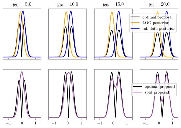
Figure 4: For the normal model with known variance, the shape of the optimal proposal distribution together with different proposal distributions for different values of the outlier $y_{30}$. Top row: LOO posterior and full data posterior. Bottom row: Split proposal distribution from equation (9).

C.2 Normal Model: Randomly Generated Data

In Figure 5, the results of Figure 2 are replicated, but now the normally distributed observations $y_{1}$ to $y_{29}$ are different for each Stan run. The results are in principle similar to those discussed in Section 3.1.

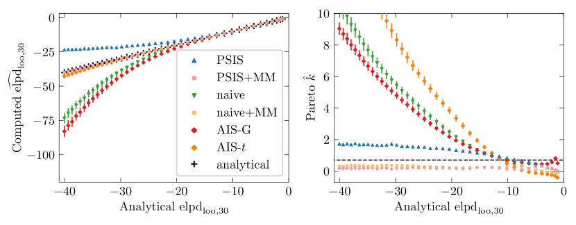
Figure 5: Computed log predictive density estimates of the left out observation $y_{30}$ for different values between $y_{30}=0$ and $y_{30}=20$ in the Gaussian model of Section 3.1. The black crosses depict the analytical LOO predictive density. The sampling results are averaged from 100 independent Stan runs, and the error bars represent $95\%$ intervals of the mean across these runs. For every Stan run, the observations $y_{1}$ to $y_{29}$ are randomly re-generated.

C.3 Importance weighted moment matching without Pareto smoothing

In Table 3, we show similar results as in Table 2, but the importance weighted moment matching does not use Pareto smoothing to smooth the importance weights during adaptation (Vehtari et al., 2019c, ).

Table 3: Upper part: Numbers of LOO folds with Pareto $\hat{k}$ diagnostic above 0.7 when the models are fitted to the full data set (lower is better). Lower part: Average run times in seconds for different algorithms. Column PSIS corresponds to using the full data posterior directly as the proposal distribution. Columns PSIS+MM and IS+MM correspond to importance weighted moment matching with an without Pareto smoothed importance weights, respectively.

Folds with $\hat{k}>0.7$

Data and model	Draws	PSIS	PSIS+MM	IS+MM
Section 3.2:	$2000$	15.2	0	0
Roach data	$4000$	14.7	0	0
Poisson regression model	$8000$	14.2	0	0
Section 3.3:	$2000$	14.0	0	0.5
Correlated Predictor Variables	$4000$	13.8	0	0.3
Linear regression model	$8000$	13.4	0	0.2
Section 3.4:	$1000$	34.8	20.1	20.7
Ovarian cancer data ($n<p$)	$2000$	36.1	19.6	19.9
Logistic regression model	$4000$	34.8	16.2	17.1
	$8000$	34.0	11.4	13.5

Computation times (seconds)

Data and model	Draws	PSIS	PSIS+MM	IS+MM
Section 3.2:	$2000$	0	39	39
Roach data	$4000$	0	70	70
Poisson regression model	$8000$	0	140	140
Section 3.3	$2000$	0	52	51
Correlated Predictor Variables	$4000$	0	114	114
Linear regression model	$8000$	0	346	340
Section 3.4	$1000$	0	199	181
Ovarian cancer data ($n<p$)	$2000$	0	372	344
Logistic regression model	$4000$	0	1558	1566
	$8000$	0	3733	3816

References

- Akyildiz and Míguez, (2019) Akyildiz, Ö. D. and Míguez, J. (2019). Convergence rates for optimised adaptive importance samplers. arXiv preprint arXiv:1903.12044.
- Ando and Tsay, (2010) Ando, T. and Tsay, R. (2010). Predictive likelihood for Bayesian model selection and averaging. International Journal of Forecasting, 26(4):744–763.
- Bernardo, (1979) Bernardo, J. M. (1979). Expected information as expected utility. The Annals of Statistics, pages 686–690.
- Bernardo and Smith, (1994) Bernardo, J. M. and Smith, A. F. (1994). Bayesian theory. Wiley.
- Betancourt, (2017) Betancourt, M. (2017). A Conceptual Introduction to Hamiltonian Monte Carlo. arXiv preprint arXiv:1701.02434.
- Bugallo et al., (2017) Bugallo, M. F., Elvira, V., Martino, L., Luengo, D., Miguez, J., and Djuric, P. M. (2017). Adaptive importance sampling: the past, the present, and the future. IEEE Signal Processing Magazine, 34(4):60–79.
- Bugallo et al., (2015) Bugallo, M. F., Martino, L., and Corander, J. (2015). Adaptive importance sampling in signal processing. Digital Signal Processing, 47:36–49.
- Cappé et al., (2008) Cappé, O., Douc, R., Guillin, A., Marin, J.-M., and Robert, C. P. (2008). Adaptive importance sampling in general mixture classes. Statistics and Computing, 18(4):447–459.
- Cappé et al., (2004) Cappé, O., Guillin, A., Marin, J.-M., and Robert, C. P. (2004). Population Monte Carlo. Journal of Computational and Graphical Statistics, 13(4):907–929.
- Carpenter et al., (2017) Carpenter, B., Gelman, A., Hoffman, M. D., Lee, D., Goodrich, B., Betancourt, M., Brubaker, M., Guo, J., Li, P., and Riddell, A. (2017). Stan: A probabilistic programming language. Journal of statistical software, 76(1).
- Chatterjee et al., (2018) Chatterjee, S., Diaconis, P., et al. (2018). The sample size required in importance sampling. The Annals of Applied Probability, 28(2):1099–1135.
- Cornuet et al., (2012) Cornuet, J.-M., Marin, J.-M., Mira, A., and Robert, C. P. (2012). Adaptive multiple importance sampling. Scandinavian Journal of Statistics, 39(4):798–812.
- Elvira et al., (2015) Elvira, V., Martino, L., Luengo, D., and Bugallo, M. F. (2015). Efficient multiple importance sampling estimators. IEEE Signal Processing Letters, 22(10):1757–1761.
- Elvira et al., (2016) Elvira, V., Martino, L., Luengo, D., and Bugallo, M. F. (2016). Heretical multiple importance sampling. IEEE Signal Processing Letters, 23(10):1474–1478.
- Elvira et al., (2017) Elvira, V., Martino, L., Luengo, D., and Bugallo, M. F. (2017). Improving population Monte Carlo: Alternative weighting and resampling schemes. Signal Processing, 131:77–91.
- Elvira et al., (2019) Elvira, V., Martino, L., Luengo, D., Bugallo, M. F., et al. (2019). Generalized multiple importance sampling. Statistical Science, 34(1):129–155.
- Elvira et al., (2018) Elvira, V., Martino, L., and Robert, C. P. (2018). Rethinking the effective sample size. arXiv preprint arXiv:1809.04129.
- Epifani et al., (2008) Epifani, I., MacEachern, S. N., and Peruggia, M. (2008). Case-deletion importance sampling estimators: Central limit theorems and related results. Electronic Journal of Statistics, 2:774–806.
- Feng et al., (2018) Feng, M. B., Maggiar, A., Staum, J., and Wächter, A. (2018). Uniform convergence of sample average approximation with adaptive multiple importance sampling. In 2018 Winter Simulation Conference (WSC), pages 1646–1657. IEEE.
- Geisser and Eddy, (1979) Geisser, S. and Eddy, W. F. (1979). A predictive approach to model selection. Journal of the American Statistical Association, 74(365):153–160.
- Gelfand, (1996) Gelfand, A. E. (1996). Model determination using sampling-based methods. In Gilks, W. R., Richardson, S., and Spiegelhalter, D. J., editors, Markov Chain Monte Carlo in Practice, pages 145–162. Chapman & Hall.
- Gelfand et al., (1992) Gelfand, A. E., Dey, D. K., and Chang, H. (1992). Model determination using predictive distributions with implementation via sampling-based methods (with discussion). In Bernardo, J. M., Berger, J. O., Dawid, A. P., and Smith, A. F. M., editors, Bayesian Statistics 4, pages 147–167. Oxford University Press.
- Gelman and Hill, (2006) Gelman, A. and Hill, J. (2006). Data analysis using regression and multilevel/hierarchical models. Cambridge university press.
- Giordano et al., (2019) Giordano, R., Stephenson, W., Liu, R., Jordan, M., and Broderick, T. (2019). A swiss army infinitesimal jackknife. In The 22nd International Conference on Artificial Intelligence and Statistics, pages 1139–1147.
- Gneiting and Raftery, (2007) Gneiting, T. and Raftery, A. E. (2007). Strictly proper scoring rules, prediction, and estimation. Journal of the American Statistical Association, 102(477):359–378.
- Good, (1952) Good, I. (1952). Rational decisions. Journal of the Royal Statistical Society: Series B (Methodological), 14(1):107–114.
- Havran and Sbert, (2014) Havran, V. and Sbert, M. (2014). Optimal combination of techniques in multiple importance sampling. In Proceedings of the 13th ACM SIGGRAPH International Conference on Virtual-Reality Continuum and its Applications in Industry, pages 141–150.
- He and Owen, (2014) He, H. Y. and Owen, A. B. (2014). Optimal mixture weights in multiple importance sampling. arXiv preprint arXiv:1411.3954.
- Hernández-Lobato et al., (2010) Hernández-Lobato, D., Hernández-Lobato, J. M., and Suárez, A. (2010). Expectation propagation for microarray data classification. Pattern recognition letters, 31(12):1618–1626.
- Hesterberg, (1995) Hesterberg, T. (1995). Weighted average importance sampling and defensive mixture distributions. Technometrics, 37(2):185–194.
- Hesterberg, (1988) Hesterberg, T. C. (1988). Advances in importance sampling. PhD thesis, Stanford University.
- Hoeting et al., (1999) Hoeting, J. A., Madigan, D., Raftery, A. E., and Volinsky, C. T. (1999). Bayesian model averaging: a tutorial. Statistical science, pages 382–401.
- Hoffman and Gelman, (2014) Hoffman, M. D. and Gelman, A. (2014). The No-U-Turn sampler: adaptively setting path lengths in Hamiltonian Monte Carlo. Journal of Machine Learning Research, 15(1):1593–1623.
- Ionides, (2008) Ionides, E. L. (2008). Truncated importance sampling. Journal of Computational and Graphical Statistics, 17(2):295–311.
- Kahn and Marshall, (1953) Kahn, H. and Marshall, A. W. (1953). Methods of reducing sample size in Monte Carlo computations. Journal of the Operations Research Society of America, 1(5):263–278.
- Kappen and Ruiz, (2016) Kappen, H. J. and Ruiz, H. C. (2016). Adaptive importance sampling for control and inference. Journal of Statistical Physics, 162(5):1244–1266.
- Koblents and Míguez, (2015) Koblents, E. and Míguez, J. (2015). A population Monte Carlo scheme with transformed weights and its application to stochastic kinetic models. Statistics and Computing, 25(2):407–425.
- Kong, (1992) Kong, A. (1992). A note on importance sampling using standardized weights. University of Chicago, Dept. of Statistics, Tech. Rep, 348.
- Krueger et al., (2019) Krueger, F., Lerch, S., Thorarinsdottir, T. L., and Gneiting, T. (2019). Probabilistic forecasting and comparative model assessment based on Markov chain Monte Carlo output. arXiv preprint arXiv:1608.06802.
- Martino et al., (2017) Martino, L., Elvira, V., and Louzada, F. (2017). Effective sample size for importance sampling based on discrepancy measures. Signal Processing, 131:386–401.
- Martino et al., (2015) Martino, L., Elvira, V., Luengo, D., and Corander, J. (2015). An adaptive population importance sampler: Learning from uncertainty. IEEE Transactions on Signal Processing, 63(16):4422–4437.
- Meng and Schilling, (2002) Meng, X.-L. and Schilling, S. (2002). Warp bridge sampling. Journal of Computational and Graphical Statistics, 11(3):552–586.
- Miguez et al., (2018) Miguez, J., Mariño, I. P., and Vázquez, M. A. (2018). Analysis of a nonlinear importance sampling scheme for Bayesian parameter estimation in state-space models. Signal Processing, 142:281–291.
- Owen and Zhou, (2000) Owen, A. and Zhou, Y. (2000). Safe and effective importance sampling. Journal of the American Statistical Association, 95(449):135–143.
- Owen, (2013) Owen, A. B. (2013). Monte Carlo theory, methods and examples.
- Peruggia, (1997) Peruggia, M. (1997). On the variability of case-deletion importance sampling weights in the Bayesian linear model. Journal of the American Statistical Association, 92(437):199–207.
- (47) Piironen, J. and Vehtari, A. (2017a). Comparison of Bayesian predictive methods for model selection. Statistics and Computing, 27(3):711–735.
- (48) Piironen, J. and Vehtari, A. (2017b). Sparsity information and regularization in the horseshoe and other shrinkage priors. Electron. J. Statist., 11(2):5018–5051.
- R Core Team, (2020) R Core Team (2020). R: A Language and Environment for Statistical Computing. R Foundation for Statistical Computing, Vienna, Austria.
- Rischard et al., (2018) Rischard, M., Jacob, P. E., and Pillai, N. (2018). Unbiased estimation of log normalizing constants with applications to Bayesian cross-validation. arXiv preprint arXiv:1810.01382.
- Robert and Casella, (2013) Robert, C. and Casella, G. (2013). Monte Carlo statistical methods. Springer Science & Business Media.
- Roberts et al., (2004) Roberts, G. O., Rosenthal, J. S., et al. (2004). General state space Markov chains and MCMC algorithms. Probability surveys, 1:20–71.
- Rubino and Tuffin, (2009) Rubino, G. and Tuffin, B. (2009). Rare event simulation using Monte Carlo methods. John Wiley & Sons.
- Sbert and Elvira, (2019) Sbert, M. and Elvira, V. (2019). Generalizing the balance heuristic estimator in multiple importance sampling. arXiv preprint arXiv:1903.11908.
- Sbert and Havran, (2017) Sbert, M. and Havran, V. (2017). Adaptive multiple importance sampling for general functions. The Visual Computer, 33(6-8):845–855.
- Sbert et al., (2016) Sbert, M., Havran, V., and Szirmay-Kalos, L. (2016). Variance analysis of multi-sample and one-sample multiple importance sampling. Computer Graphics Forum, 35(7):451–460.
- Schummer et al., (1999) Schummer, M., Ng, W. V., Bumgarner, R. E., Nelson, P. S., Schummer, B., Bednarski, D. W., Hassell, L., Baldwin, R. L., Karlan, B. Y., and Hood, L. (1999). Comparative hybridization of an array of 21 500 ovarian cdnas for the discovery of genes overexpressed in ovarian carcinomas. Gene, 238(2):375–385.
- Stan Development Team, (2018) Stan Development Team (2018). RStan: the R interface to Stan, version 2.17.3.
- Veach and Guibas, (1995) Veach, E. and Guibas, L. J. (1995). Optimally combining sampling techniques for Monte Carlo rendering. In Proceedings of the 22nd annual conference on Computer graphics and interactive techniques, pages 419–428. ACM.
- (60) Vehtari, A., Gabry, J., Magnusson, M., Yao, Y., and Gelman, A. (2019a). loo: Efficient leave-one-out cross-validation and WAIC for Bayesian models. R package version 2.2.0.
- Vehtari et al., (2017) Vehtari, A., Gelman, A., and Gabry, J. (2017). Practical Bayesian model evaluation using leave-one-out cross-validation and waic. Statistics and Computing, 27(5):1413–1432.
- (62) Vehtari, A., Gelman, A., Simpson, D., Carpenter, B., and Bürkner, P.-C. (2019b). Rank-normalization, folding, and localization: An improved for assessing convergence of MCMC. arXiv preprint arXiv:1903.08008.
- Vehtari and Lampinen, (2002) Vehtari, A. and Lampinen, J. (2002). Bayesian model assessment and comparison using cross-validation predictive densities. Neural computation, 14(10):2439–2468.
- Vehtari and Ojanen, (2012) Vehtari, A. and Ojanen, J. (2012). A survey of Bayesian predictive methods for model assessment, selection and comparison. Statistics Surveys, 6:142–228.
- (65) Vehtari, A., Simpson, D., Gelman, A., Yao, Y., and Gabry, J. (2019c). Pareto smoothed importance sampling. arXiv preprint arXiv:1507.02646.
- Zhang, (1996) Zhang, P. (1996). Nonparametric importance sampling. Journal of the American Statistical Association, 91(435):1245–1253.