Bounding the error of discretized Langevin algorithms for non-strongly log-concave targets

Abstract

In this paper, we provide non-asymptotic upper bounds on the error of sampling from a target density over $\mathbb{R}^{p}$ using three schemes of discretized Langevin diffusions. The first scheme is the Langevin Monte Carlo (LMC) algorithm, the Euler discretization of the Langevin diffusion. The second and the third schemes are, respectively, the kinetic Langevin Monte Carlo (KLMC) for differentiable potentials and the kinetic Langevin Monte Carlo for twice-differentiable potentials (KLMC2). The main focus is on the target densities that are smooth and log-concave on $\mathbb{R}^{p}$, but not necessarily strongly log-concave. Bounds on the computational complexity are obtained under two types of smoothness assumption: the potential has a Lipschitz-continuous gradient and the potential has a Lipschitz-continuous Hessian matrix. The error of sampling is measured by Wasserstein-$q$ distances. We advocate for the use of a new dimension-adapted scaling in the definition of the computational complexity, when Wasserstein-$q$ distances are considered. The obtained results show that the number of iterations to achieve a scaled-error smaller than a prescribed value depends only polynomially in the dimension.

Keywords: Approximate sampling, log-concave distributions, Langevin Monte Carlo

1 Introduction

The two most popular techniques for defining estimators or predictors in statistics and machine learning are the $M$ estimation, also known as empirical risk minimization, and the Bayesian method (leading to posterior mean, posterior median, etc.). In practice, it is necessary to devise a numerical method for computing an approximation of these estimators. Optimization algorithms are used for approximating an $M$-estimator, while Monte Carlo algorithms are employed for approximating Bayesian estimators. In statistical learning theory, over past decades, a concentrated effort was made for getting non asymptotic guarantees on the error of an optimization algorithm. For smooth optimization, sharp results were obtained in the case of strongly convex and convex cases (Bubeck, 2015), the case of non-convex smooth optimization being much more delicate (Jain and Kar, 2017). As for Monte Carlo algorithms, past three years or so witnessed considerable progress on theory of sampling from strongly log-concave densities. Some results for (non strongly) concave densities were obtained as well. However, to the best of our knowledge, there is no paper providing a systematic account on the error bounds for sampling from (non strongly) log-concave densities over unbounded domains. The main goal of this paper is to fill this gap.

A good starting point for accomplishing the aforementioned task is perhaps a result from (Durmus et al., 2019) for the sampling error measured by the Kullback-Leibler divergence. The result is established for the Langevin Monte Carlo (LMC) algorithm, which is the “sampling analogue” of the gradient descent. Let $\pi:\mathbb{R}^{p}\to[0,+\infty)$ be a probability density function (with respect to Lebesgue’s measure) given by

$$\pi(\boldsymbol{\theta})=\frac{e^{-f(\boldsymbol{\theta})}}{\int_{\mathbb{R}^{p}}e^{-f(\boldsymbol{v})}d\boldsymbol{v}}.$$ (1)

for a potential function $f$. The goal of sampling is to generate a random vector in $\mathbb{R}^{p}$ having a distribution close to the target distribution defined by $\pi$. In the sequel, we will make repeated use of the moments $\mu_{k}(\pi)=\mathbf{E}_{\boldsymbol{\vartheta}\sim\pi}[\|\boldsymbol{\vartheta}\|_{2}^{k}]^{1/k}$, where $\|\boldsymbol{v}\|_{q}=(\sum_{j}|v_{j}|^{q})^{1/q}$ is the usual $\ell_{q}$-norm for any $q\geq 1$. When there is no risk of confusion, we will write $\mu_{k}$ instead of $\mu_{k}(\pi)$.

To define the LMC algorithm, we need a sequence of positive parameters $\boldsymbol{h}=\{h_{k}\}_{k\in\mathbb{N}}$, referred to as the step-sizes and an initial point $\boldsymbol{\vartheta}_{0,\boldsymbol{h}}\in\mathbb{R}^{p}$ that may be deterministic or random. The successive iterations of the LMC algorithm are given by the update rule

$$\boldsymbol{\vartheta}_{k+1,\boldsymbol{h}}=\boldsymbol{\vartheta}_{k,\boldsymbol{h}}-h_{k+1}\nabla f(\boldsymbol{\vartheta}_{k,\boldsymbol{h}})+\sqrt{2h_{k+1}}\;\boldsymbol{\xi}_{k+1};\qquad k=0,1,2,\ldots$$ (2)

where $\boldsymbol{\xi}_{1},\ldots,\boldsymbol{\xi}_{k},\ldots$ is a sequence of independent, and independent of $\boldsymbol{\vartheta}_{0,\boldsymbol{h}}$, centered Gaussian vectors with identity covariance matrices. Let $\nu_{K}$ denote the distribution of the $K$-th iterate of the LMC algorithm, assuming that all the step-sizes are equal ($h_{k}=h$ for every $k\in\mathbb{N}$) and the initial point is $\boldsymbol{\vartheta}_{0,h}=\mathbf{0}_{p}$. We will also define the distribution $\bar{\nu}_{K}=(\nicefrac{{1}}{{K}})\sum_{k=1}^{K}\nu_{k}$, obtained by choosing uniformly at random one of the elements of the sequence $\{\boldsymbol{\vartheta}_{1,\boldsymbol{h}},\ldots,\boldsymbol{\vartheta}_{K,\boldsymbol{h}}\}$. It is proved in (Durmus et al., 2019, Cor. 7) that if the gradient $\nabla f$ is Lipschitz continuous with the Lipschitz constant $M$, then for every $K\in\mathbb{N}$, the Kullback-Leibler divergence between $\bar{\nu}_{K}$ and $\pi$ satisfies

$$D_{\rm KL}(\bar{\nu}_{K}\|\pi)\leq\frac{\mu^{2}_{2}(\pi)}{2Kh}+Mph,\qquad D_{\rm KL}(\bar{\nu}_{K}^{\rm opt}\|\pi)\leq\sqrt{\frac{2Mp}{K}}\,\mu_{2}(\pi).$$ (3)

Note that the second inequality above is derived from the first one by using the step-size $h_{\rm opt}=\mu_{2}(\pi)/\sqrt{2KMp}$ obtained by minimizing the right hand side of the first inequality. Therefore, if we assume that the second-order moment $\mu_{2}$ of $\pi$ satisfies the condition $M\mu_{2}^{2}\leq\kappa p^{\beta}$, for some dimension-free positive constants $\beta$ and $\kappa$, we get

$$D_{\rm KL}(\bar{\nu}_{K}^{\rm opt}\|\pi)\leq\sqrt{\frac{2\kappa p^{1+\beta}}{K}}.$$ (4)

A natural measure of complexity of the LMC with averaging is, for every $\varepsilon>0$, the number of gradient evaluations that is sufficient for getting a sampling error bounded from above by $\varepsilon$. From the last display, taking into account the Pinsker inequality, $d_{\rm TV}(\bar{\nu}_{K},\pi)\leq\sqrt{D_{\rm KL}(\bar{\nu}_{K},\pi)/2}$, and the fact that each iterate of the LMC requires one evaluation of the gradient of $f$, we obtain the following result. The number of gradient evaluations $K_{\rm LMCa,TV}(p,\varepsilon)$ sufficient for the total-variation-error of the LMC with averaging (hereafter, LMCa) to be smaller than $\varepsilon$ is

$$K_{\rm LMCa,TV}(p,\varepsilon)=\frac{\kappa p^{1+\beta}}{2\varepsilon^{4}}.$$ (5)

The main goal of the present work is to provide this type of bounds on the complexity of various versions of the Langevin algorithm under different measures of the quality of sampling. The most important feature that we wish to uncover is the explicit dependence of the complexity $K(\varepsilon)$ on the dimension $p$, the inverse-target-precision $1/\varepsilon$ and the condition number $\kappa$. We will focus only on those measures of quality of sampling that can be directly used for evaluating the quality of approximating expectations.

The main contributions of this paper are:

• Bounds on the sampling error measured in the Wasserstein $W_{q}$-distance (for $q\in[1,2]$) in two settings: (a) convex and gradient-Lipschitz potential and (b) convex, gradient-Lipschitz and Hessian-Lipschitz potential. Tight bounds are established for the strong-convexified versions of three algorithms: Langevin Monte Carlo, kinetic Langevin Monte Carlo and kinetic Langevin Monte Carlo for twice-differentiable potentials.

• Bounds on the moments of log-concave distributions, especially in the settings where the potential function $f$ is strongly convex inside a ball and (weakly) convex everywhere else, or strongly convex outside a ball and (weakly) convex everywhere else. These bounds are low-degree polynomials in dimension and in the other relevant parameters.

• Upper bounds on the mixing time of the aforementioned three versions of the Langevin algorithm, obtained by combining the $W_{q}$-error bounds and moment evaluations.

The remainder of the paper is structured as follows. We begin in Section 2 by introducing the sampling methods based on the Langevin diffusion and by formulating the main assumptions that are used throughout this work. Section 3 and Section 4 contain, respectively, a discussion on the choice of the complexity measure and an overview of our main contributions. Relation to prior work is discussed in Section 5. Section 6 and Section 7 contain formal statements and proofs of the main error- and complexity-bounds for the vanilla and the kinetic Langevin, respectively. Upper bounds for the moments of two classes of log-concave distributions are presented in Section 8. We conclude with a discussion in Section 9.

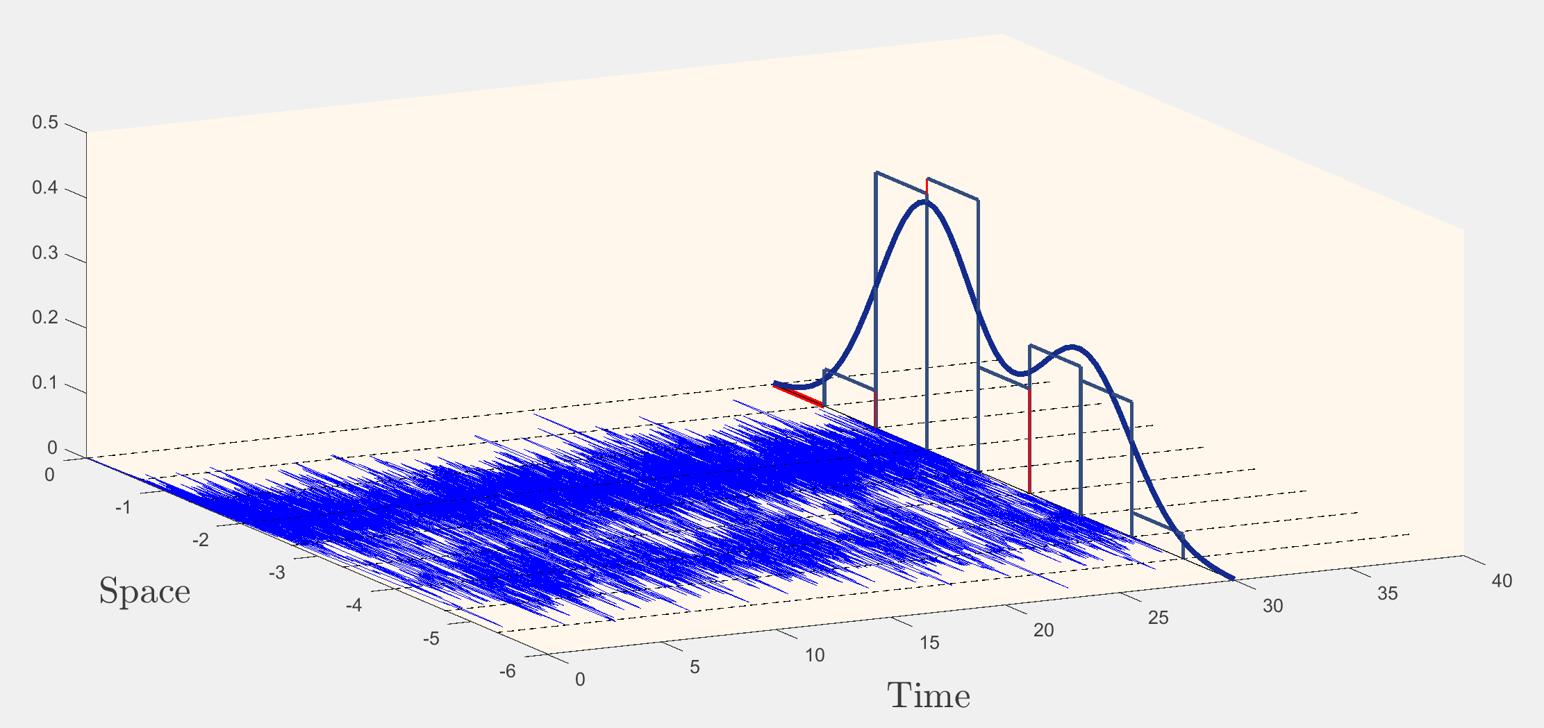
Figure 1: Illustration of Langevin dynamics. The blue lines represent different paths of a Langevin process. We see that the histogram of the state at time $t=30$ is close to the target density (the dark blue line).

2 Further precisions on the analyzed methods

Since our main motivation for considering the sampling problem comes from applications in statistics and machine learning, we will focus on the Monge-Kantorovich-Wasserstein distances $W_{q}$ defined by

$$W_{q}(\nu,\nu^{\prime}) =\inf\Big{\{}\mathbf{E}[\|\boldsymbol{\vartheta}-\boldsymbol{\vartheta}^{\prime}\|_{2}^{q}]^{1/q}:\boldsymbol{\vartheta}\sim\nu\text{ and }\boldsymbol{\vartheta}^{\prime}\sim\nu^{\prime}\Big{\}},\qquad q\geq 1.$$ (6)

The infimum above is over all the couplings between $\nu$ and $\nu^{\prime}$. In view of the Hölder inequality, the mapping $q\mapsto W_{q}(\nu,\nu^{\prime})$ is increasing for every pair $(\nu,\nu^{\prime})$.

Our main contributions are upper bounds on quantities of the form $W_{q}(\nu_{K},\pi)$where $\pi$ is a log-concave target distribution and $\nu_{K}$ is the distribution of the $K$th iterate of various discretization schemes of Langevin diffusions. More precisely, we consider two types of Langevin processes: the kinetic Langevin diffusion and the vanilla Langevin diffusion. The latter is the highly overdamped version of the former, see (Nelson, 1967). The Langevin diffusion, having $\pi$ as invariant distribution, is defined as a solution to the stochastic differential equation

$$d\boldsymbol{L}_{t}^{\textup{{LD}}}=-\nabla f(\boldsymbol{L}_{t}^{\textup{{LD}}})\,dt+\sqrt{2}\,d\boldsymbol{W}_{t},\qquad t\geq 0,$$ (7)

where $\boldsymbol{W}$ is a $p$-dimensional standard Brownian motion independent of the initial value $\boldsymbol{L}_{0}$. An illustration of this process is given in Figure 1. The LMC algorithm presented in (2) is merely the Euler-Maruyama discretization of the process $\boldsymbol{L}$. The kinetic Langevin diffusion $\{\boldsymbol{L}_{t}^{\textup{{KLD}}}:t\geq 0\}$, also known as the second-order Langevin process, is defined by

$$d\begin{bmatrix}\boldsymbol{V}_{t}\\ \boldsymbol{L}_{t}^{\textup{{KLD}}}\end{bmatrix} =\begin{bmatrix}-(\gamma\boldsymbol{V}_{t}+\nabla f(\boldsymbol{L}_{t}^{\textup{{KLD}}}))\\ \boldsymbol{V}_{t}\end{bmatrix}\,dt+\sqrt{2\gamma}\begin{bmatrix}\mathbf{I}_{p}\\ \mathbf{0}_{p\times p}\end{bmatrix}\,d\boldsymbol{W}_{t},\qquad t\geq 0,$$ (8)

where $\gamma>0$ is the friction coefficient. The process $\boldsymbol{V}_{t}$ is often called the velocity process since the second row in (8) implies that $\boldsymbol{V}_{t}$ is the time derivative of $\boldsymbol{L}_{t}^{\textup{{KLD}}}$. The continuous-time Markov process $(\boldsymbol{L}_{t}^{\textup{{KLD}}},\boldsymbol{V}_{t})$ is positive recurrent and has a unique invariant distribution, which has the following density with respect to the Lebesgue measure on $\mathbb{R}^{2p}$:

$$p_{*}(\boldsymbol{\theta},\boldsymbol{v})\propto\exp\Big{\{}-f(\boldsymbol{\theta})-\frac{1}{2}\|\boldsymbol{v}\|_{2}^{2}\Big{\}},\qquad\boldsymbol{\theta}\in\mathbb{R}^{p},\ \boldsymbol{v}\in\mathbb{R}^{p}.$$ (9)

If $(\boldsymbol{L},\boldsymbol{V})$ is a pair of random vectors drawn from the joint density $p_{*}$, then $\boldsymbol{L}$ and $\boldsymbol{V}$ are independent, $\boldsymbol{L}$ is distributed according to the target $\pi$, whereas $\boldsymbol{V}$ is a standard Gaussian vector. Therefore, at equilibrium, the random variable $\boldsymbol{L}_{t}^{\textup{{KLD}}}$ has the target distribution $\pi$.

Time-discretized versions of Langevin diffusion processes (7) and (8) are used for (approximately) sampling from $\pi$. In order to guarantee that the discretization error is not too large, as well as that the process $\{\boldsymbol{L}_{t}\}$ converges fast enough to its invariant distribution, we need to impose some assumptions on $f$. In the present work, we will assume that either Conditions 1, 2 or Conditions 1, 2, 3 presented below are satisfied.

Condition 1

The function $f$ is continuously differentiable on $\mathbb{R}^{p}$ and its gradient $\nabla f$ is $M$-Lipschitz for some $M>0$: $\|\nabla f(\boldsymbol{\theta})-\nabla f(\boldsymbol{\theta}^{\prime})\|_{2}\leq M\|\boldsymbol{\theta}-\boldsymbol{\theta}^{\prime}\|_{2}$ for all $\boldsymbol{\theta},\boldsymbol{\theta}^{\prime}\in\mathbb{R}^{p}$.

From now on, we will always assume that the Langevin (vanilla or kinetic) diffusion under consideration has the initial point $\boldsymbol{L}_{0}=\mathbf{0}$. Some of the conditions presented below implicitly require that this initialization is not too far away from the “center” of the target distribution $\pi$. In many statistical problems where $\pi$ is the Bayesian posterior, one can come close to these assumptions by shifting the distribution using a simple initial estimator.

Condition 2

The function $f$ is convex on $\mathbb{R}^{p}$. Furthermore, for some positive constants $D$ and $\beta$, we have $\mu^{2}_{2}(\pi)=\mathbf{E}_{\boldsymbol{\vartheta}\sim\pi}[\|\boldsymbol{\vartheta}\|_{2}^{2}]\leq Dp^{\beta}$.

Under Condition 2, the centered second moment of $\pi$ scales polynomially with the dimension with power $\beta>0$, while the flatness of the distribution is controlled by the parameter $D>0$. Remarkably, Condition 2 implies that all the moments $\{\mu_{q}(\pi)\}_{q\geq 1}$ scale polynomially with $p$, provided that $\mathbf{E}_{\vartheta\sim\pi}[\|\boldsymbol{\vartheta}\|_{2}^{2}]$ also does. This fact is a consequence of Borell’s lemma (Giannopoulos et al., 2014, Theorem  2.4.6 ), stating that for any $q\geq 1$, there is a numerical constant $B_{q}$ that depends only on $q$ such that $\mu_{q}(\pi)\leq B_{q}\mu_{2}(\pi)$. An attempt to provide optimized constants in this inequality is stated in Lemma 5.

In the sequel, we show that the smoothness and the flatness of $\pi$ have a combined impact on the sampling error considered. It turns out that the important parameter with respect to the hardness of the sampling problem is the product

$$\kappa:=MD.$$ (10)

For $m$-strongly convex functions $f$, Condition 2 is satisfied with $D=1/m$ and $\beta=1$, according to Brascamp-Lieb inequality (Brascamp and Lieb, 1976). In this case, the parameter $\kappa=M/m$ is referred to as the condition number. We will show that Condition 2 is also satisfied for functions $f$ that are convex everywhere and strongly convex inside a ball, as well as for functions $f$ that are convex everywhere and strongly convex only outside a ball.

In the next assumption, we use notation $\|\mathbf{M}\|$ for the spectral norm (the largest singular value) of a matrix $\mathbf{M}$.

Condition 3

The function $f$ is twice differentiable in $\mathbb{R}^{p}$ with a $M_{2}$-Lipschitz Hessian $\nabla^{2}f$ for some $M_{2}>0$: $\|\nabla^{2}f(\boldsymbol{\theta})-\nabla^{2}f(\boldsymbol{\theta}^{\prime})\|\leq M_{2}\|\boldsymbol{\theta}-\boldsymbol{\theta}^{\prime}\|_{2}$ for all $\boldsymbol{\theta},\boldsymbol{\theta}^{\prime}\in\mathbb{R}^{p}$.

Condition 3 ensures further smoothness of the potential $f$. When it holds, the Lipschitz continuity of the Hessian and the flatness of $\pi$ also have a combined impact on the sampling error. A second important parameter with respect to the hardness of the sampling problem in such a case is the product

$$\kappa_{2}:=M_{2}^{2/3}D.$$ (11)

The case of an $m$-strongly convex function $f$ has been studied in several recent papers. As a matter of fact, global strong convexity implies exponentially fast mixing of processes (7) and (8), with dimension-free rates $e^{-mt}$ and $e^{-mt/(M+m)^{1/2}}$, respectively. When only (weak) convexity is assumed, such results do not hold in general. Therefore, the strategy we adopt here consists in sampling from a distribution that is provably close to the target, but has the advantage of being strongly log-concave.

More precisely, for some small positive $\alpha$, the surrogate potential is defined by $f_{\alpha}(\boldsymbol{\theta}):=f(\boldsymbol{\theta})+\alpha\|\boldsymbol{\theta}\|_{2}^{2}/2$. Therefore, the corresponding surrogate distribution has the density

$$\pi_{\alpha}(\boldsymbol{\theta}):=\frac{e^{-f_{\alpha}(\boldsymbol{\theta})}}{\int_{\mathbb{R}^{p}}e^{-f_{\alpha}(\boldsymbol{v})}d\boldsymbol{v}}.$$ (12)

We stress the fact that the quadratic penalty $\alpha\|\boldsymbol{\theta}\|_{2}^{2}/2$ added to the potential $f$ is centered at the origin. This is closely related to the fact that the diffusion is assumed to have the origin as initial point, and also to the fact that the origin is assumed here to be a good guess of the “center” of $\pi$. The parameter $\alpha$, together with the step-size $\boldsymbol{h}$, is considered as a tuning parameter of the algorithms to be calibrated. Large values of $\alpha$ will result in fast convergence to $\pi_{\alpha}$ but a poor approximation of $\pi$ by $\pi_{\alpha}$. On the other hand, smaller values of $\alpha$ will lead to a small approximation error but also slow convergence. The next result quantifies the approximation of $\pi$ by $\pi_{\alpha}$, for different distances.

Proposition 1

For any $\alpha\geq 0$ and $q\in[1,+\infty)$, there is a numerical constant $C_{q}$ depending only on $q$ such that

$$d_{\rm TV}(\pi,\pi_{\alpha})\leq\alpha\mu^{2}_{2}(\pi),\qquad W_{q}^{q}(\pi,\pi_{\alpha})\leq C_{q}\alpha\mu_{2}(\pi)^{q+2}.$$ (13)

Here the constant $C_{q}$ can be bounded for every $q$. In particular, $C_{1}\leq 11$ and $C_{2}\leq 111$.

This result allows us to control the bias induced by replacing the target distribution by the surrogate one and paves the way for choosing the “optimal” $\alpha$ by minimizing an upper bound on the sampling error. We draw the attention of the reader to the fact that, for $W_{q}$ distance, the dependence on $\alpha$ of the upper bound is $\alpha^{1/q}$, which slows down when $q$ increases (recall that $\alpha$ is a small parameter). This explains the deterioration with increasing $q$ of the complexity bounds presented in forthcoming sections. Let us define the constant

$$C_{q}=\inf\{C:W_{q}^{q}(\pi,\pi_{\alpha})\leq C\alpha\mu_{2}(\pi)^{q+2},\ \forall\,\pi\textup{ log-concave}\},$$ (14)

which will repeatedly appear in the statements of the theorems.

3 How to measure the complexity of a sampling scheme?

We have already introduced the notation $K_{\sf Alg,Crit}(p,\varepsilon)$, the number of iterations that guarantee that algorithm Alg has an error—measured by criterion Crit—smaller than $\varepsilon$. If we choose a criterion, this quantity can be used to compare two methods, the iterates of which have comparable computational complexity. For example, LMC and KLMC being discretized versions of the Langevin process (7) and the kinetic Langevin process (8), respectively, are such that one iteration requires one evaluation of $\nabla f$ and generation of one realization of a Gaussian vector of dimension $p$ or $2p$. Thus, the iterations are of comparable computational complexity and, therefore, it is natural to prefer LMC if $2K_{\rm LMC,\sf Crit}(p,\varepsilon)\leq K_{\rm KLMC,\sf Crit}(p,\varepsilon)$ and to prefer KLMC if the opposite inequality is true.

A delicate question that has not really been discussed in literature is a notion of complexity that allows to compare the quality of a given sampling method for two different criteria. To be more precise, assume that we are interested in the LMC algorithm and wish to figure out whether it is “more difficult” to perform approximate sampling for the TV-distance or for the Wasserstein distance. It is a well-known fact that the TV-distance induces the uniform strong convergence of measures whereas the Wasserstein distances induce the weak convergence. Therefore, at least intuitively, approximate sampling for the TV-distance should be harder than approximate sampling for the Wasserstein distance. However, under Condition 1 and $m$-strong convexity of $f$, the available results for the LMC provide the same order of magnitude, $p/\varepsilon^{2}$, both for $K_{\rm LMC,TV}$ (Dalalyan, 2017b; Durmus and Moulines, 2019) and $K_{{\rm LMC},W_{2}}$ (Durmus and Moulines, 2019; Dalalyan and Tsybakov, 2009). The point we want to put forward is that the origin of this discrepancy between the intuitions and mathematical results is the inappropriate scaling of the target accuracy in the definition of $K_{{\rm LMC},W_{2}}$.

To further justify the importance of choosing the right scaling of the target accuracy, let us make the following observation. The total-variation distance, on the one hand, serves to approximate probabilities, which are adimensional and scale-free quantities belonging to the interval $[0,1]$. The Wasserstein distances, on the other hand, are useful for approximating moments, the latter depending both on the dimension and on the scale. For this reason, we suggest the following definition of the analogue of $K$ in the case of Wasserstein distances:

$$K_{{\sf Alg},W_{q}}(p,\varepsilon)=\min\{k\in\mathbb{N}:W_{q}(\nu_{k}^{\sf Alg},\pi)\leq\varepsilon\mu_{2}(\pi),\ \forall\,\pi\in\mathscr{P}\},$$ (15)

where ${\sf Alg}$ is a Markov Chain Monte Carlo or another method of sampling, $k$ is generally the number of calls to the oracle and $\mathscr{P}$ is a class of target distributions. Examples of oracle call are the evaluation of the gradient of the potential at a given point or the computation of the product of the Hessian of $f$ at a given point and a given vector. Note also that $\mu_{2}(\pi)$ is the $W_{2}$ distance between the Dirac mass at the origin and the target distribution.

Definition (15), as opposed to those used in prior work, has the advantage of being scale invariant and reflecting the fact that we deal with objects that might be large if the dimension is large. Note that the idea of scaling the error in order to make the complexity measure scale-invariant has been recently used in (Tat Lee et al., 2018; Baker et al., 2019) as well. Indeed, in the context of $m$-strongly log-concave distributions, Tat Lee et al. (2018) propose to find the smallest $k$ such that $W_{2}(\nu_{k}^{\sf Alg},\pi)\leq\varepsilon/\sqrt{m}$. This is close to our proposal, since in the case of $m$-strongly log-concave distributions, it follows from the Brascamp-Lieb inequality that $\sup_{\pi}{\mu_{2}(\pi)}=\sqrt{p/m}$ (the sup is attained for Gaussian distributions).

4 Overview of main contributions

In this work, we analyze three methods, LMC, KLMC (Cheng et al., 2018b) and KLMC2 (Dalalyan and Riou-Durand, 2020), applied to the strong-convexified potential $f_{\alpha}(\boldsymbol{\theta})=f(\boldsymbol{\theta})+(\alpha/2)\|\boldsymbol{\theta}\|_{2}^{2}$ in order to cope with the lack of strong convexity. We briefly recall these algorithms and present a summary of the main contributions of this work.

4.1 Considered Markov chain Monte-Carlo methods

We first recall the definition of the Langevin Monte Carlo algorithms. For the LMC algorithm introduced in (2), we will only use the constant step-size form, the update rule of which is given by

$$\boldsymbol{\vartheta}_{k+1}=(1-\alpha h)\boldsymbol{\vartheta}_{k}-h\nabla f(\boldsymbol{\vartheta}_{k})+\sqrt{2h}\;\boldsymbol{\xi}_{k+1};\qquad k=0,1,2,\ldots \alpha$$ (-LMC)

where $\boldsymbol{\xi}_{1},\ldots,\boldsymbol{\xi}_{k},\ldots$ is a sequence of mutually independent, independent of $\boldsymbol{\vartheta}_{0}$, centered Gaussian vectors with covariance matrices equal to identity. We will refer to this version of the LMC algorithm as $\alpha$-LMC.

We now recall the definition of the first and second-order Kinetic Langevin Monte Carlo algorithms. We suppose that, for some initial distribution $\nu_{0}$ chosen by the user, both KLMC and KLMC2 algorithms start from $(\boldsymbol{v}_{0},\boldsymbol{\vartheta}_{0})\sim\mathcal{N}(\mathbf{0}_{p},\mathbf{I}_{p})\otimes\nu_{0}$. Before stating the update rules, we specify the structure of the random perturbation generated at each step. In what follows, $\{(\boldsymbol{\xi}_{k}^{(1)},\boldsymbol{\xi}_{k}^{(2)},\boldsymbol{\xi}_{k}^{(3)},\boldsymbol{\xi}_{k}^{(4)}):k\in\mathbb{N}\}$ will stand for a sequence of iid $4p$-dimensional centered Gaussian vectors, independent of the initial condition $(\boldsymbol{v}_{0},\boldsymbol{\vartheta}_{0})$.

To specify the covariance structure of these Gaussian variables, we define two sequences of functions $(\psi_{k})$ and $(\varphi_{k})$ as follows. For every $t>0$, let $\psi_{0}(t)=e^{-\gamma t}$, then for every $k\in\mathbb{N}$, define $\psi_{k+1}(t)=\int_{0}^{t}\psi_{k}(s)\,ds$ and $\varphi_{k+1}(t)=\int_{0}^{t}e^{-\gamma(t-s)}\psi_{k}(s)\,ds$. Now, let us denote by $\xi_{k,j}$ for the $j$-th component of the vector $\boldsymbol{\xi}_{k}$ (a scalar), and assume that for any fixed $k$, the $4$-dimensional random vectors $\{(\xi_{k,j}^{(1)},\xi_{k,j}^{(2)},\xi_{k,j}^{(3)},\xi_{k,j}^{(4)}):1\leq j\leq p\}$ are iid with the covariance matrix

$$\mathbf{C}_{h,\gamma}=\int_{0}^{h}[\psi_{0}(t);\,\psi_{1}(t);\,\varphi_{2}(t);\,\varphi_{3}(t)]^{\top}[\psi_{0}(t);\,\psi_{1}(t);\,\varphi_{2}(t);\,\varphi_{3}(t)]\,dt.$$ (16)

The KLMC algorithm, introduced by Cheng et al. (2018b), is a sampler derived from a suitable time-discretization of the kinetic diffusion. When applied to the strong-convexified potential $f_{\alpha}$, for a step-size $h>0$, its update rule reads as follows

$$\begin{bmatrix}\boldsymbol{v}_{k+1}\\[4.0pt] \boldsymbol{\vartheta}_{k+1}\end{bmatrix} =\begin{bmatrix}\psi_{0}(h)\boldsymbol{v}_{k}-\psi_{1}(h)(\nabla f(\boldsymbol{\vartheta}_{k})+\alpha\boldsymbol{\vartheta}_{k})\\[4.0pt] \boldsymbol{\vartheta}_{k}+\psi_{1}(h)\boldsymbol{v}_{k}-\psi_{2}(h)(\nabla f(\boldsymbol{\vartheta}_{k})+\alpha\boldsymbol{\vartheta}_{k})\end{bmatrix}+\sqrt{2\gamma}\begin{bmatrix}\boldsymbol{\xi}_{k+1}^{(1)}\\[4.0pt] \boldsymbol{\xi}_{k+1}^{(2)}\end{bmatrix}. \alpha$$ (-KLMC)

Roughly speaking, this formula is obtained from (8) by replacing the function $t\mapsto\nabla f(\boldsymbol{L}_{t})$ by a piecewise constant approximation. Such an approximation is made possible by the fact that $f$ is gradient-Lipschitz.

It is natural to expect that further smoothness of $f$ may allow one to improve upon the aforementioned piecewise constant approximation. This is done by the KLMC2 algorithm, introduced by Dalalyan and Riou-Durand (2020), which takes advantage of the existence and smoothness of the Hessian of $f$ in order to use a local-linear approximation. At any iteration $k\in\mathbb{N}$ with a current value $\boldsymbol{\vartheta}_{k}$, define the gradient $\boldsymbol{g}_{k,\alpha}=\nabla f(\boldsymbol{\vartheta}_{k})+\alpha\boldsymbol{\vartheta}_{k}$ and the Hessian $\mathbf{H}_{k,\alpha}=\nabla^{2}f(\boldsymbol{\vartheta}_{k})+\alpha\mathbf{I}_{p}$. When applied to the modified strongly convex potential $f_{\alpha}$, for $h>0$, the update rule of the KLMC2 algorithm is

$$\begin{bmatrix}\boldsymbol{v}_{k+1}\\[4.0pt] \boldsymbol{\vartheta}_{k+1}\end{bmatrix} =\begin{bmatrix}\psi_{0}(h)\boldsymbol{v}_{k}-\psi_{1}(h)\boldsymbol{g}_{k,\alpha}-\varphi_{2}(h)\mathbf{H}_{k,\alpha}\boldsymbol{v}_{k}\\[4.0pt] \boldsymbol{\vartheta}_{k}+\psi_{1}(h)\boldsymbol{v}_{k}-\psi_{2}(h)\boldsymbol{g}_{k,\alpha}-\varphi_{3}(h)\mathbf{H}_{k,\alpha}\boldsymbol{v}_{k}\end{bmatrix}+\sqrt{2\gamma}\begin{bmatrix}\boldsymbol{\xi}_{k+1}^{(1)}-\mathbf{H}_{k,\alpha}\boldsymbol{\xi}_{k+1}^{(3)}\\[4.0pt] \boldsymbol{\xi}_{k+1}^{(2)}-\mathbf{H}_{k,\alpha}\boldsymbol{\xi}_{k+1}^{(4)}\end{bmatrix}. \alpha$$ (-KLMC2)

Notice that if we apply KLMC2 with $\mathbf{H}_{k,\alpha}=0$, we recover the KLMC algorithm. These two algorithms, derived from the kinetic Langevin diffusion, will be referred to as $\alpha$-KLMC and $\alpha$-KLMC2.

4.2 Summary of the obtained complexity bounds

Without going into details here, we mention in the tables below the order of magnitude of the number of iterations required by different algorithms for getting an error bounded by $\varepsilon$ for various metrics. For improved legibility, we do not include logarithmic factors and report the order of magnitude of $K_{\square,\square}(p,\varepsilon)$ in the case when the parameter $\beta$ in Condition 2 is fixed to a particular value. We present hereafter the case where $\beta=1$, which is of particular interest as discussed in Section 8.

$\beta=1$	LMCa	$\alpha$-LMC		$\alpha$-KLMC	$\alpha$-KLMC2
Cond.	1-2	1-2	1-3	1-2	1-3
$W_{2}$	$-$	$\kappa p^{2}/\varepsilon^{6}\ \hphantom{\color[rgb]{0.9453125,0.2578125,0.19921875}\boldsymbol{\square}}$	$(\kappa_{2}^{1.5}p^{0.5}+\kappa^{1.5}){p^{2}}/{\varepsilon^{5}}$	$\kappa^{1.5}p^{2}/\varepsilon^{5}$	$\kappa^{0.5}{\kappa_{2}}^{1.5}p^{2}/\varepsilon^{4}$
$W_{1}$	$-$	$\kappa p^{2}/\varepsilon^{4}\ \hphantom{\color[rgb]{0.9453125,0.2578125,0.19921875}\boldsymbol{\square}}$	$(\kappa_{2}^{1.5}p^{0.5}+\kappa^{1.5}){p^{2}}/{\varepsilon^{3}}$	$\kappa^{1.5}p^{2}/\varepsilon^{3}$	$\kappa^{0.5}{\kappa_{2}}^{1.5}p^{2}/\varepsilon^{2}$
$d_{\rm TV}$	$\kappa p^{2}/\varepsilon^{4}\ {\color[rgb]{0,0.34765625,0.703125}\boldsymbol{\triangle}}$	$\kappa^{2}p^{3}/\varepsilon^{4}\ {\color[rgb]{0.9453125,0.2578125,0.19921875}\boldsymbol{\square}}$	$-$	$-$	$-$

The results indicated by ${\color[rgb]{0,0.34765625,0.703125}\boldsymbol{\triangle}}$ describe the behavior of the Langevin Monte Carlo with averaging established in (Durmus et al., 2019, Cor. 7). To date, these results have the best known dependence (under conditions 1 and 2 only) on $p$. The results indicated by ${\color[rgb]{0.9453125,0.2578125,0.19921875}\boldsymbol{\square}}$ summarize the behavior of the Langevin Monte Carlo established in (Dalalyan, 2017b). All the remaining cells of the table are filled in by the results obtained in the present work. One can observe that the results for $W_{1}$ are strictly better than those for $W_{2}$. Similar hierarchy was already reported in (Majka et al., 2020, Remark 1.9). It is also worth mentioning here, that using Metropolis-Hastings adjustment of the LMC (termed MALA), Dwivedi et al. (2018); Chen et al. (2020) obtained the complexity

$$K_{\rm MALA,TV}(p,\varepsilon)=O\bigg{(}\frac{p^{2}\kappa^{3/2}}{\varepsilon^{3/2}}\,\log\big{(}p\kappa/\varepsilon\big{)}\bigg{)}.$$ (17)

It is still an open question whether this type of result can be proved for Wasserstein distances.

We would also like to comment on the relation between the third and the fourth columns of the table, corresponding to the $\alpha$-LMC algorithm under different sets of assumptions. The result for the more constrained Hessian-Lipschitz case is not always better than the result when only gradient Lipschitzness is assumed. For instance, for $W_{2}$, the latter is better than the former when $\kappa\lesssim(\kappa_{2}^{1.5}p^{0.5}+\kappa^{1.5})\varepsilon$, which is equivalent to $M\lesssim(M_{2}p^{1/2}+M^{3/2})D^{1/2}\varepsilon$. At a very high level, this reflects the fact that when the condition number is large, the Hessian-Lipschitzness does not help to get an improved result. Note that the same phenomenon occurs in the strongly log-concave case.

4.3 The general approach based on a log-strongly-concave surrogate

We have already mentioned that the strategy we adopt here is the one described in (Dalalyan, 2017b), consisting of replacing the potential of the target density by a strongly convex surrogate. Prior to instantiating this approach to various sampling algorithms under various conditions and error measuring distances, we provide here a more formal description of it. In the remaining ${\sf dist}$ is a general distance on the set of all probability measures.

We will denote by $\nu_{k,\alpha}^{{\sf Alg}}$ the distribution of the random vector obtained after performing $k$ iterations of the algorithm ${\sf Alg}$ with the surrogate potential $f_{\alpha}(\boldsymbol{\theta})=f(\boldsymbol{\theta})+\alpha\|\boldsymbol{\theta}\|_{2}^{2}/2$. Our first goal is to establish an upper bound on the distance between the sampling distribution $\nu_{k,\alpha}^{{\sf Alg}}$ and the target $\pi$. The methods we analyze here depend on the step-size $h$, as they are discretizations of continuous-time diffusion processes. Thus, the obtained bound will depend on $h$. This bound should be so that one can make it arbitrarily small by choosing small $\alpha$ and $h$ and a large value of $k$. In a second stage, the goal is to exploit the obtained error-bounds in order to assess the order of magnitude of the computational complexity $K$, defined in Section 3, as a function of $p$, $\varepsilon$ and the condition number $\kappa$.

To achieve this goal, we first use the triangle inequality

$${\sf dist}(\nu_{k,\alpha}^{{\sf Alg}},\pi)\leq{\sf dist}(\nu_{k,\alpha}^{{\sf Alg}},\pi_{\alpha})+{\sf dist}(\pi_{\alpha},\pi).$$ (18)

Then, the second term of the right hand side of the last displayed equation is bounded using Proposition 1. Finally, the distance between the sampling density $\nu_{k,\alpha}^{{\sf Alg}}$ and the surrogate $\pi_{\alpha}$ is bounded using the prior work on sampling for log-strongly-concave distributions. Optimizing over $\alpha$ leads to the best bounds on precision and complexity.

5 Prior work

Mathematical analysis of MCMC methods defined as discretizations of diffusion processes is an active area of research since several decades. Important early references are (Roberts and Tweedie, 1996; Roberts and Rosenthal, 1998; Roberts and Stramer, 2002; Douc et al., 2004) and the references therein. Although those papers do cover the multidimensional case, the guarantees they provide do not make explicit the dependence on the dimension. In a series of work analyzing ball walk and hit-and-run MCMCs, Lovasz and Vempala (2006); Lovász and Vempala (2006) put forward the importance of characterizing the dependence of the number of iterations on the dimension of the state space.

More recently, Dalalyan (2017b) advocated for analyzing MCMCs obtained from continuous time diffusion processes by decomposing the error into two terms: a non-stationarity error of the continuous-time process and a discretization error. A large number of works applied this kind of approach in various settings. (Bubeck et al., 2018; Durmus and Moulines, 2017, 2019; Durmus et al., 2018) improved the results obtained by Dalalyan and extended them in many directions including non-smooth potentials and variable step-sizes. While previous work studied the sampling error measured by the total variation and Waserstein distances, (Cheng and Bartlett, 2018) proved that similar results hold for the Kulback-Leibler divergence. (Cheng et al., 2018b, a; Dalalyan and Riou-Durand, 2020) investigated the case of a kinetic Langevin diffusion, showing that it leads to improved dependence on the dimension. A promising line of related research, initiated by (Wibisono, 2018; Bernton, 2018), is to consider the sampling distributions as a gradient flow in a space of measures. The benefits of this approach were demonstrated in (Durmus et al., 2019; Ma et al., 2019).

Motivated by applications in Statistics and Machine Learning, many recent papers developed theoretical guarantees for stochastic versions of algorithms, based on noisy gradients, see (Baker et al., 2019; Chatterji et al., 2018; Dalalyan and Karagulyan, 2019; Dalalyan, 2017a; Zou et al., 2019; Raginsky et al., 2017) and the references therein. A related topic is non-asymptotic guarantees for the Hamiltonian Monte Carlo (HMC). There is a growing literature on this in recent years, see (Mangoubi and Smith, 2017; Tat Lee et al., 2018; Chen and Vempala, 2019; Mangoubi and Smith, 2019) and the references therein.

In all these results, the dependence of the number of iterations on the inverse precision is polynomial. (Dwivedi et al., 2018; Chen et al., 2020; Mangoubi and Vishnoi, 2019) proved that one can reduce this dependence to logarithmic by using Metropolis adjusted versions of the algorithms.

6 Precision and computational complexity of the LMC

In this section, we present non-asymptotic upper bounds in the (non-strongly) convex case for the suitably adapted LMC algorithm for Wasserstein and bounded-Lipschitz error measures under two sets of assumptions: Conditions 1-2 and Conditions 1-3. To refer to these settings, we will call them “Gradient-Lipschitz” and “Hessian-Lipschitz”, respectively. The main goal is to provide a formal justification of the rates included in columns 2 and 3 of the table presented in Section 4.2. To ease notation, and since there is no risk of confusion, we write $\mu_{2}$ instead $\mu_{2}(\pi)$.

6.1 The Gradient-Lipschitz setting

First we consider the Gradient-Lipschitz setting and give explicit conditions on the parameters $\alpha$, $h$ and $K$ to have a theoretical guarantee on the sampling error, measured in the Wasserstein distance, of the LMC algorithm.

Theorem 1

Suppose that the potential function $f$ is convex and satisfies Condition 1. Let $q\in[1,2]$. Then, for every $\alpha\leq M/20$ and $h\leq 1/(M+\alpha)$, we have

$$W_{q}(\nu_{K}^{\alpha\text{\sf-LMC}},\pi) \leq\underbrace{{\mu_{2}}(1-\alpha h)^{K/2}}_{\begin{subarray}{c}\text{\rm error due to the }\\[2.0pt] \text{\rm time finiteness}\end{subarray}}+\underbrace{\left({2.1hMp/\alpha}\right)^{1/2}}_{\text{\rm discretization error}}+\underbrace{\left(C_{q}\alpha\mu_{2}^{q+2}\right)^{1/q}}_{\begin{subarray}{c}\text{\rm error due to the lack}\\[2.0pt] \text{\rm of strong-convexity}\end{subarray}},$$ (19)

where $C_{q}$ is a dimension free constant given by (14).

The proof of this result is postponed to the end of this section. Let us consider its consequences in the cases $q=1$ and $q=2$ presented in the table of Section 4.2. The general strategy is to choose the value of $\alpha$ by minimizing the sum of the discretization error and the error caused by the lack of strong convexity. Then, the parameter $h$ is chosen so that the sum of the two aforementioned errors is smaller than $99\%$ of the target precision $\varepsilon{\mu_{2}}$. Finally, the number of iterations $K$ is selected in such a way that the error due to the time finiteness is also smaller than $1\%$ of the target precision.

Implementing this strategy for $q=1$ and $q=2$, we get the optimized value of $\alpha$ and the corresponding value of $h$,

$q=1$	$q=2$
$\displaystyle\alpha=\frac{(2.1hMp)^{1/3}}{44^{2/3}\mu_{2}^{2}}\quad h=\frac{\varepsilon^{3}}{322Mp}$	$\displaystyle\alpha=\frac{(2.1hMp)^{1/2}}{111^{1/2}\mu_{2}^{2}}\quad h=\frac{\varepsilon^{4}}{3900Mp}$

These values of $\alpha$ and $h$ satisfy the conditions imposed in Theorem 1. They imply that the computational complexity of the method, for $\nu_{0}=\delta_{0}$ (the Dirac mass at the origin), is given by

$$K_{\alpha\text{-LMC},W_{1}}(p,\varepsilon) \leq\frac{2}{\alpha h}\log\Big{(}\frac{100W_{2}(\nu_{0},\pi_{\alpha})}{\varepsilon{\mu_{2}}}\Big{)}\leq 4.3\times 10^{4}M\frac{\mu^{2}_{2}p}{\varepsilon^{4}}\log(100/\varepsilon)$$ (20)

$$K_{\alpha\text{-LMC},W_{2}}(p,\varepsilon) \leq\frac{2}{\alpha h}\log\Big{(}\frac{100W_{2}(\nu_{0},\pi_{\alpha})}{\varepsilon{\mu_{2}}}\Big{)}\leq 3.6\times 10^{6}M\frac{\mu_{2}^{2}p}{\varepsilon^{6}}\log(100/\varepsilon).$$ (21)

In both inequalities, the second passage is due to the monotone behaviour of the function $\alpha\mapsto\mu_{2}(\pi_{\alpha})$. This property, formulated in Lemma 1, implies that

$$W_{2}(\delta_{0},\pi_{\alpha})=\mu_{2}(\pi_{\alpha})\leq\mu_{2}(\pi).$$ (22)

Combining Condition 2, $M\mu_{2}^{2}(\pi)\leq\kappa p^{\beta}$, with the last display, we check that $K_{\alpha\text{-LMC},W_{1}}(p,\varepsilon)\leq C\kappa(p^{1+\beta}/\varepsilon^{4})\log(100/\varepsilon)$ and $K_{\alpha\text{-LMC},W_{2}}(p,\varepsilon)\leq C\kappa(p^{1+\beta}/\varepsilon^{6})\log(100/\varepsilon)$. For $\beta=1$, this matches well with the rates reported in the table of Section 4.2. Unfortunately, the numerical constant $C$, just like the factors $4.3\times 10^{4}$ and $3.6\times 10^{6}$ in the last display, is too large to be useful for practical purposes. Getting similar bounds with better numerical constants is an open question. The same remark applies to all the results presented in the subsequent sections.

Proof of Theorem 1

To ease notation, we write $\nu_{K}$ instead of $\nu_{K}^{\alpha\text{\sf-LMC}}$. The triangle inequality and the monotonicity of $W_{q}$ with respect to $q$ imply that

$$W_{q}(\nu_{K},\pi) \leq W_{2}(\nu_{K},\pi_{\alpha})+W_{q}(\pi_{\alpha},\pi).$$ (23)

Recall that $\pi_{\alpha}$ is $\alpha$-strongly log-concave and has $f_{\alpha}$ as its potential function. By definition, $f_{\alpha}$ has also a Lipschitz continuous gradient with the Lipschitz constant at most $M+\alpha$. As we assume that $h\leq{1}/{(M+\alpha)}$, we can apply (Durmus et al., 2019, Theorem 9). It implies that

$$W_{2}(\nu_{K},\pi_{\alpha}) \leq(1-\alpha h)^{K/2}W_{2}(\nu_{0},\pi_{\alpha})+\left({2h(M+\alpha)p/\alpha}\right)^{1/2}$$ (24)

$$\leq(1-\alpha h)^{K/2}W_{2}(\nu_{0},\pi_{\alpha})+\left({2.1hMp/\alpha}\right)^{1/2}.$$ (25)

The last inequality is true due to the fact that $\alpha\leq M/20$. Combining this inequality with Proposition 1, we obtain

$$W_{q}(\nu_{K},\pi) \leq(1-\alpha h)^{K/2}W_{2}(\nu_{0},\pi_{\alpha})+({2.1hMp/\alpha})^{1/2}+W_{q}(\pi_{\alpha},\pi)$$ (26)

$$\leq\mu_{2}(\pi_{\alpha})(1-\alpha h)^{K/2}+({2.1hMp/\alpha})^{1/2}+\big{(}C_{q}\alpha\mu_{2}^{q+2}\big{)}^{1/q}.$$ (27)

Thus, applying (22), we get the claim of the theorem. $\blacksquare$

6.2 The Hessian-Lipschitz setting

It has been noticed by Durmus and Moulines (2019), see also (Dalalyan and Karagulyan, 2019, Theorem 5), that if the potential $f$ has a Lipschitz-continuous Hessian matrix, then the LMC algorithm, without any modification, is more accurate than in the Gradient-Lipschitz setting. These improvements were obtained under the condition of strong convexity of the potential, showing that the computational complexity drops down from $p/\varepsilon^{2}$ to $p/\varepsilon$. The goal of this section is to understand how this additional smoothness assumption impacts the computational complexity of the $\alpha$-LMC algorithm.

Theorem 2

Suppose that the potential function $f$ satisfies conditions 1 and 3. Let $q\in[1,2]$. For every $\alpha\leq M/20$ and $h\leq 1/(M+\alpha)$, we have

$$W_{q}(\nu_{K}^{\alpha\text{\sf-LMC}}\!,\pi) \leq\underbrace{\mu_{2}(1-\alpha h)^{K}}_{\begin{subarray}{c}\text{\rm error due to the}\\[2.0pt] \text{\rm time finiteness}\end{subarray}}+\underbrace{\frac{M_{2}hp}{2\alpha}+\frac{2.8M^{3/2}hp^{1/2}}{\alpha}}_{\text{\rm discretization error}}+\underbrace{\left(C_{q}\alpha\mu_{2}^{q+2}\right)}_{\begin{subarray}{c}\text{\rm error due to the lack}\\[2.0pt] \text{\rm of strong-convexity}\end{subarray}}\!{}^{1/q},$$ (28)

where $C_{q}$ is a dimension free constant given by (14).

In order to provide more insight on the complexity bounds implied by the latter result, let us instantiate it for $q=1$ and $q=2$. Optimizing the sum of the two last error terms with respect to $\alpha$, then choosing this sum to be equal to $0.99\varepsilon{\mu_{2}}$, we arrive at the following values

$q=1$	$q=2$
$\displaystyle\alpha=\left(\frac{hQp}{44\mu_{2}^{3}}\right)^{1/2}\quad h=\frac{\varepsilon^{2}}{45\mu_{2}Qp}$	$\displaystyle\alpha=\frac{(hQp)^{2/3}}{(111\mu_{2}^{4})^{1/3}}\quad h=\frac{\varepsilon^{3}}{387\mu_{2}Qp}$

Here $Q$ is defined as $(M_{2}+5.6M^{3/2}p^{-1/2})$. These values of $\alpha$ and $h$ satisfy the conditions imposed in Theorem 2. They imply that the computational complexity of the method, for $\nu_{0}=\delta_{0}$ (the Dirac mass at the origin), is given by

$$K_{\alpha\text{-LMC},W_{1}}(p,\varepsilon) \leq\frac{2}{\alpha h}\log\Big{(}\frac{100W_{2}(\nu_{0},\pi_{\alpha})}{\varepsilon{\mu_{2}}}\Big{)}\leq 2\times 10^{3}\mu_{2}^{3}Q(p/\varepsilon^{3})\log(100/\varepsilon)$$ (29)

$$K_{\alpha\text{-LMC},W_{2}}(p,\varepsilon) \leq\frac{2}{\alpha h}\log\Big{(}\frac{100W_{2}(\nu_{0},\pi_{\alpha})}{\varepsilon{\mu_{2}}}\Big{)}\leq 9.9\times 10^{4}\mu_{2}^{3}Q(p/\varepsilon^{5})\log(100/\varepsilon).$$ (30)

Combining Condition 2 and the last display, we check that

$$K_{\alpha\text{-LMC},W_{1}}(p,\varepsilon) \leq C\varepsilon^{-3}(\kappa_{2}^{3/2}p^{(2+3\beta)/2}+\kappa^{3/2}p^{(1+3\beta)/2})\log(100/\varepsilon),$$ (31)

$$K_{\alpha\text{-LMC},W_{2}}(p,\varepsilon) \leq C\varepsilon^{-5}(\kappa_{2}^{3/2}p^{(2+3\beta)/2}+\kappa^{3/2}p^{(1+3\beta)/2})\log(100/\varepsilon).$$ (32)

The latter is true, since by definition $\kappa_{2}$ is equal to $M_{2}^{2/3}D$. For $\beta=1$, this matches well with the rates reported in the table of Section 4.2.

Proof of Theorem 2

We repeat the same steps as in the proof of Theorem 1, except that instead of (Durmus et al., 2019, Theorem 9) we use (Dalalyan and Karagulyan, 2019, Theorem 5). To ease notation, we write $\nu_{K}$ instead of $\nu_{K}^{\alpha\text{\sf-LMC}}$. One easily checks that $\pi_{\alpha}$ is $\alpha$-strongly log-concave with potential function $f_{\alpha}$. Furthermore, the latter is $(M+\alpha)$-gradient-Lipschitz and $M_{2}$-Hessian-Lipschitz. Therefore, for $h\leq{2}/{(M+\alpha)}$, Theorem 5 from (Dalalyan and Karagulyan, 2019) implies that

$$W_{2}(\nu_{K},\pi_{\alpha}) \leq(1-\alpha h)^{K}W_{2}(\nu_{0},\pi_{\alpha})+\frac{M_{2}hp}{2\alpha}+\frac{13(M+\alpha)^{3/2}hp^{1/2}}{5\alpha}$$ (33)

$$\leq(1-\alpha h)^{K}W_{2}(\nu_{0},\pi_{\alpha})+\frac{M_{2}hp}{2\alpha}+\frac{2.8M^{3/2}hp^{1/2}}{\alpha},$$ (34)

where the second inequality follows from the fact that $\alpha\leq M/20$. The triangle inequality and the monotonicity of $W_{q}$ with respect to $q$ yield $W_{q}(\nu_{K},\pi)\leq W_{2}(\nu_{K},\pi_{\alpha})+W_{q}(\pi_{\alpha},\pi)$, which leads to

$$W_{q}(\nu_{K},\pi) \leq{\mu_{2}(\pi_{\alpha})}(1-\alpha h)^{K}+\frac{M_{2}hp}{2\alpha}+\frac{2.8M^{3/2}hp^{1/2}}{\alpha}+W_{q}(\pi,\pi_{\alpha}).$$ (35)

Replacing the last term above by its upper bound provided by Proposition 1 and applying (22), we get the claimed result. $\blacksquare$

7 Precision and computational complexity of KLMC and KLMC2

Several recent studies showed that for some classes of targets, including the strongly log-concave densities, the sampling error of discretizations of the kinetic Langevin diffusion scales better with the large dimension than discretizations of the Langevin diffusion. However, the dependence of the available bounds on the condition number is better for the Langevin diffusion. In this section we show a similar behavior in the case of (non-strongly) log-concave densities. This is done by providing quantitative upper bounds on the error of sampling using the kinetic Langevin process.

Theorem 3

Suppose that the potential function $f$ satisfies Condition 1. Let $q\in[1,2]$. Then for every $\alpha\leq M/20$, $\gamma\geq\sqrt{M+2\alpha}$ and $h\leq\alpha/(4\gamma(M+\alpha))$, we have

$$W_{q}(\nu_{K}^{\alpha\text{\sf-KLMC}},\pi) \leq\underbrace{\sqrt{2}\,\mu_{2}\left(1-\frac{3\alpha h}{4\gamma}\right)^{K}}_{\begin{subarray}{c}\text{\rm error due to the time finiteness}\end{subarray}}+\underbrace{1.5Mp^{1/2}(h/\alpha)}_{\text{\rm discretization error}}+\underbrace{\left(C_{q}\alpha\mu_{2}^{q+2}\right)^{1/q}}_{\begin{subarray}{c}\text{\rm error due to the lack}\\[2.0pt] \text{\rm of strong-convexity}\end{subarray}}.$$ (36)

where $C_{q}$ is a dimension free constant given by (14).

The proof of this result is postponed to the end of this section. Since the contraction rate is an increasing function of $\gamma$, we choose its lowest possible value achieved for $\gamma=\sqrt{M+2\alpha}$. Then the strategy is the same as for the previous section, that is to choose the value of $\alpha$ by minimizing the sum of the discretization error and the error caused by the lack of strong convexity. Then, the parameter $h$ is chosen so that the sum of the two aforementioned errors is smaller than $99\%$ of the target precision $\varepsilon\mu_{2}$. The number of iterations $K$ is selected in such a way that the error due to the time finiteness is also smaller than $1\%$ of the target precision. Implementing this strategy for $q=1$ and $q=2$, we get the optimized value of $\alpha$ and the corresponding value of $h$,

$q=1$	$q=2$
$\displaystyle\alpha=\frac{(1.5hMp^{1/2})^{1/2}}{(21\mu_{2}^{3})^{1/2}}\quad h=\frac{\varepsilon^{2}}{143M\mu_{2}p^{1/2}}$	$\displaystyle\alpha=\frac{(3hMp^{1/2})^{2/3}}{(111\mu_{2}^{4})^{1/3}}\quad h=\frac{\varepsilon^{4}}{1200M\mu_{2}p^{1/2}}$

These values of $\alpha$ and $h$ satisfy the conditions imposed in Theorem 3. They imply that the computational complexity of the method, for $\nu_{0}=\delta_{0}$ (the Dirac mass), is given by

$$K_{\alpha\text{-KLMC},W_{1}}(p,\varepsilon) \leq\frac{4\gamma}{3\alpha h}\log\Big{(}\frac{150}{\varepsilon}\Big{)}\leq 9.2\times 10^{3}(M\mu_{2}^{2})^{3/2}(p^{1/2}/\varepsilon^{3})\log(150/\varepsilon)$$ (37)

$$K_{\alpha\text{-KLMC},W_{2}}(p,\varepsilon) \leq\frac{4\gamma}{3\alpha h}\log\Big{(}\frac{150}{\varepsilon}\Big{)}\leq 4.4\times 10^{5}(M\mu_{2}^{2})^{3/2}(p^{1/2}/\varepsilon^{5})\log(150/\varepsilon).$$ (38)

Recall that Condition 2 implies $M\mu_{2}^{2}\leq\kappa p^{\beta}$. Combining this inequality with the last display, we check that

$$K_{\alpha\text{-KLMC},W_{q}}(p,\varepsilon) \leq C\kappa^{3/2}(p^{(1+3\beta)/2}/\varepsilon^{2q+1})\log(150/\varepsilon),\qquad q=1,2.$$ (39)

For $\beta=1$, this matches well with the rates reported in the table of Section 4.2.

Proof of Theorem 3

To ease notation, we write $\nu_{K}$ instead of $\nu_{K}^{\alpha\text{\sf-KLMC}}$. The triangle inequality and the monotonicity of $W_{q}$ with respect to $q$ imply that $W_{q}(\nu_{K},\pi)\leq W_{2}(\nu_{K},\pi_{\alpha})+W_{q}(\pi_{\alpha},\pi)$. Recall that $\pi_{\alpha}$ is a $\alpha$-strongly log-concave distribution with potential function $f_{\alpha}$. By definition, $f_{\alpha}$ has also a Lipschitz continuous gradient with the Lipschitz constant at most $M+\alpha$. As we assumed that $\alpha\leq M/20$, $\gamma\geq\sqrt{M+2\alpha}$ and $h\leq\alpha/(4\gamma(M+\alpha))$, we can apply (Dalalyan and Riou-Durand, 2020, Theorem 2). The latter implies that

$$W_{2}(\nu_{K},\pi_{\alpha}) \leq\sqrt{2}(1-3\alpha h/(4\gamma))^{K}W_{2}(\nu_{0},\pi_{\alpha})+\sqrt{2}(M+\alpha)p^{1/2}(h/\alpha)$$ (40)

$$\leq\sqrt{2}\,\mu_{2}(\pi_{\alpha})(1-3\alpha h/(4\gamma))^{K}+1.5Mp^{1/2}(h/\alpha).$$ (41)

The last inequality is true thanks to the fact that $\alpha\leq M/20$. Thus, (22) yields

$$W_{q}(\nu_{K},\pi) \leq\sqrt{2}\,\mu_{2}(\pi)(1-3\alpha h/(4\gamma))^{K}+1.5Mp^{1/2}(h/\alpha)+W_{q}(\pi_{\alpha},\pi).$$ (42)

Owing to Proposition 1, the last term of the last display can be bounded by $(C_{q}\alpha\mu_{2}^{q+2})^{1/q}$. This completes the proof. $\blacksquare$

The rest of this section is devoted to the sampling guarantees for the KLMC2 algorithm. Recall that this algorithm requires accurate evaluations of the Hessian of the potential function $f$ to be available at each given point.

Theorem 4

Suppose that the potential function $f$ satisfies conditions 1 and 3. Let $q\in[1,2]$ and $Q=M_{2}+M^{3/2}p^{-1/2}$. Then, for every $\alpha,h,\gamma>0$ such that

$$\alpha\leq\frac{M}{20},\qquad\gamma\geq\sqrt{M+2\alpha},\qquad h\leq\frac{\alpha}{5\gamma(M+\alpha)}\bigvee\frac{\alpha}{4M_{2}\sqrt{5p}},$$ (43)

we have

$$W_{q}(\nu_{K}^{\alpha\text{\sf-KLMC2}},\pi)\leq\underbrace{\sqrt{2}\,\mu_{2}\left(1-\frac{\alpha h}{4\gamma}\right)^{K}\!\!\!}_{\begin{subarray}{c}\textup{error due to the}\\[2.0pt] \textup{time finiteness}\end{subarray}} +\underbrace{\frac{2h^{2}Qp}{\alpha}+\frac{1.6}{\sqrt{M}}\exp\left\{-\frac{(\alpha/h)^{2}}{160M_{2}^{2}}\right\}}_{\textup{discretization error}}+\underbrace{\left(C_{q}\alpha\mu_{2}^{q+2}\right)^{1/q}\!\!\!}_{\begin{subarray}{c}\textup{ error due to the lack}\\[2.0pt] \textup{ of strong-convexity}\end{subarray}},$$ (44)

where $C_{q}$ is a dimension free constant given by (14).

The proof of this result is postponed to the end of this section. The contraction rate is an increasing function of $\gamma$, therefore we choose its lowest possible value achieved for $\gamma=\sqrt{M+2\alpha}$. In this case the strategy for finding $h$ and $\alpha$ is slightly different from the previous ones. Here, we first choose the parameter $h$ so that the two terms of the discretization error are respectively bounded by $1\%$ and $2\%$ of the target precision $\varepsilon{\mu_{2}}$. This yields the following choice for the time step $h$:

$$h=\alpha\left(160M_{2}^{2}\log\left(\frac{160}{\varepsilon\mu_{2}\sqrt{M}}\right)\bigvee\frac{100\alpha Qp}{\varepsilon{\mu_{2}}}\right)^{-1/2}.$$ (45)

The parameter $\alpha$ is then chosen so that the error due to the lack of strong convexity is lower than $96\%$ of the target precision. Implementing this strategy for $q=1$ and $q=2$, we get the following value for $\alpha$

$q=1$	$q=2$
$\displaystyle\alpha=\frac{\varepsilon}{23\mu_{2}^{2}}$	$\displaystyle\alpha=\frac{\varepsilon^{2}}{116\mu_{2}^{2}}$

Finally, the number of iterations $K$ is selected in such a way that the error due to the time finiteness is also smaller than $1\%$ of the target precision. This yields, that

$$K=\frac{4\gamma}{\alpha h}\log\Big{(}\frac{142}{\varepsilon}\Big{)}$$ (46)

is sufficient to reach the target precision. The values of $\gamma$, $\alpha$ and $h$ imply that the computational complexity of the method is given by

$$K_{\alpha\text{-KLMC2},W_{1}}(p,\varepsilon) =2.2\times 10^{4}\,\frac{M^{1/2}M_{2}\mu_{2}^{4}}{\varepsilon^{2}}\bigg{\{}1.6\log\Big{(}\frac{160}{\varepsilon\mu_{2}\sqrt{M}}\Big{)}\bigvee\frac{Qp}{23M_{2}^{2}\mu_{2}^{3}}\bigg{\}}^{1/2}\log\Big{(}\frac{142}{\varepsilon}\Big{)}$$ (47)

$$K_{\alpha\text{-KLMC2},W_{2}}(p,\varepsilon) =5.4\times 10^{6}\,\frac{M^{1/2}M_{2}\mu_{2}^{4}}{\varepsilon^{4}}\bigg{\{}1.6\log\Big{(}\frac{160}{\varepsilon\mu_{2}\sqrt{M}}\Big{)}\bigvee\frac{\varepsilon Qp}{116M_{2}^{2}\mu_{2}^{3}}\bigg{\}}^{1/2}\log\Big{(}\frac{142}{\varepsilon}\Big{)}.$$ (48)

Since according to Condition 2, $\mu_{2}\leq Dp^{\beta}$, the last display implies that up to logarithmic factors $K_{\alpha\text{-KLMC2},W_{1}}(p,\varepsilon)$ scales as $\kappa^{1/2}\kappa_{2}^{3/2}p^{2\beta}/\varepsilon^{2}$ and $K_{\alpha\text{-KLMC2},W_{2}}(p,\varepsilon)$ scales as $\kappa^{1/2}\kappa_{2}^{3/2}p^{2\beta}/\varepsilon^{4}$. For $\beta=1$, this matches well with the rates reported in the table of Section 4.2.

Proof of Theorem 4

To ease notation, we write $\nu_{K}$ instead of $\nu_{K}^{\alpha\text{\sf-KLMC2}}$. As already checked in the proof of Theorem 2, the distribution $\pi_{\alpha}$ is $\alpha$-strongly log-concave with potential function $f_{\alpha}$. Furthermore, the latter is $(M+\alpha)$-gradient-Lipschitz and $M_{2}$-Hessian-Lipschitz. In view of (Dalalyan and Riou-Durand, 2020, Theorem 3), since the parameters $\alpha,\gamma,h>0$ are such that

$$\alpha\leq\frac{M}{20},\qquad\gamma\geq\sqrt{M+2\alpha},\qquad h\leq\frac{\alpha}{5\gamma(M+\alpha)}\bigwedge\frac{\alpha}{4M_{2}\sqrt{5p}},$$ (49)

the distribution of the KLMC2 sampler after $k$ iterates satisfies

$$W_{2}(\nu_{k},\pi_{\alpha}) \leq\sqrt{2}\,\mu_{2}(\pi_{\alpha})\left(1-\frac{\alpha h}{4\gamma}\right)^{k}+\frac{2h^{2}M_{2}p}{\alpha}+\frac{h^{2}(M+\alpha)^{3/2}\sqrt{2p}}{\alpha}$$ (50)

$$\hskip 120.92421pt+\frac{8h(M+\alpha)}{\alpha}\exp\left\{-\frac{\alpha^{2}}{160M_{2}^{2}h^{2}}\right\}$$ (51)

$$\leq\sqrt{2}\,\mu_{2}(\pi_{\alpha})\left(1-\frac{\alpha h}{4\gamma}\right)^{K}+\frac{2h^{2}(M_{2}p+M^{3/2}p^{1/2})}{\alpha}+\frac{1.6}{\sqrt{M}}\exp\left\{-\frac{(\alpha/h)^{2}}{160M_{2}^{2}}\right\},$$ (52)

where the second inequality follows from the fact that $\alpha\leq M/20$ and $h\leq\alpha/(5\gamma(M+\alpha))$. The triangle inequality and the monotonicity of $W_{q}$ with respect to $q$ yields $W_{q}(\nu_{K},\pi)\leq W_{2}(\nu_{K},\pi_{\alpha})+W_{q}(\pi_{\alpha},\pi)$, which leads to

$$W_{q}(\nu_{K},\pi) \leq\sqrt{2}\,\mu_{2}(\pi_{\alpha})\left(1-\frac{\alpha h}{4\gamma}\right)^{K}+\frac{2h^{2}Qp}{\alpha}+\frac{1.6}{\sqrt{M}}\exp\left\{-\frac{(\alpha/h)^{2}}{160M_{2}^{2}}\right\}+W_{q}(\pi,\pi_{\alpha}).$$ (53)

Replacing the last term above by its upper bound provided by Proposition 1 and applying (22), we obtain the claim of the theorem. $\blacksquare$

8 Bounding the moments

From the user’s perspective, the choice of $\alpha$ and $h$ requires the computation of the second moment of the distribution $\pi$. In most cases, this moment is an intractable integral. However, when some additional information on $\pi$ is available, this moment can be replaced by a tractable upper bound. In this section, we provide upper bounds on the moments

$$\mu_{a}^{*}:=\big{(}\mathbf{E}_{\boldsymbol{\vartheta}\sim\pi}[\|\boldsymbol{\vartheta}-\boldsymbol{\theta}^{*}\|_{2}^{a}]\big{)}^{1/a},\qquad a\geq 1,$$ (54)

centered at the minimizer of the potential $\boldsymbol{\theta}^{*}\in\text{argmin}_{\boldsymbol{\theta}\in\mathbb{R}^{p}}f(\boldsymbol{\theta})$. The knowledge of the second moment is enough to compute the mixing times presented in Section 6 and Section 7. However, providing bounds on general moments is of interest in order to highlight the dependence on the dimension, but also to obtain sharp numerical constants when the second moment is unknown. For instance, the proof of Proposition 1 shows that results for the $W_{1}$ and $W_{2}$ metrics essentially rely on some bounds over the third and fourth moments of $\pi$, which could be better understood in some specific contexts.

In this section, we investigate two particular classes of convex functions: (a) those which are $m$-strongly convex inside a ball of radius $R$ around the mode $\boldsymbol{\theta}^{*}$, and (b) those which are $m$-strongly convex outside a ball of radius $R$ around the mode $\boldsymbol{\theta}^{*}$. We provide user-friendly bounds on $\mu_{a}^{*}$ with fairly small constants. In the aforementioned two cases, if $m$ and $R$ are dimension free, we show that $\mu_{a}^{*}$ scales respectively as $p\log p$ and $(p\log p)^{1/2}$. This scaling with the dimension is sharp, up to logarithmic factors, and matches Condition 2 with $\beta=2$ for the class (a) and Condition 2 with $\beta=1$ for the class (b).

Proposition 2

Assume that for some positive numbers $m$ and $R$, we have $\nabla^{2}f(\boldsymbol{\theta})\succeq m\mathbf{I}_{p}$ for every $\boldsymbol{\theta}\in\mathbb{R}^{p}$ such that $\|\boldsymbol{\theta}-\boldsymbol{\theta}^{*}\|_{2}\leq R$. Then, for every $a\geq 2$, we have

$$\mu_{a}^{*}\leq A\vee B+\frac{3}{mR\,\Gamma(p/2)^{1/a}}$$ (55)

where

$$A=\frac{3p}{mR}\left((1+a/p)\log(1+a/p)+\log_{+}\Big{(}\frac{2M}{m^{2}R^{2}}\Big{)}\right)\quad\text{and}\quad B=\left(\frac{p}{m}\right)^{1/2}\Big{\{}2+\frac{a}{2p}\Big{\}}^{\mathds{1}_{a>2}}.$$ (56)

In the case of fixed $a$ and $p$ tending to infinity, Proposition 2 implies that

$$\mu_{a}^{*}=\widetilde{O}\bigg{(}\frac{p}{mR}\bigvee\Big{(}\frac{p}{m}\Big{)}^{1/2}\bigg{)},$$ (57)

where $\widetilde{O}$ hides constants and polylogarithmic factors. In the bound of Proposition 2, the term $A$ is the dominating one when $p/m$ is large as compared to $R^{2}$, while $B$ is the dominating term when $R^{2}$ is of a higher order of magnitude than $p/m$. The residual term $3/(mR\Gamma(p/2)^{1/a})$ goes to zero whenever $p$ or $R$ tend to infinity. If $m$ and $R$ are assumed to be dimension free constants, then $\mu^{*}_{a}$ scales as $p\log p$. This rate is optimal within a poly-log factor, which is proven in Lemma 4. Note also that when $R$ goes to infinity we exactly recover the bound of the strongly convex case proven in Lemma 2.

We now switch to bounding the moments of $\pi$ under the condition that $f$ is convex everywhere and strongly convex outside the ball of radius $R$ around $\boldsymbol{\theta}^{*}$.

Proposition 3

Assume that for some positive $m$ and $R$, we have $\nabla^{2}f(\boldsymbol{\theta})\succeq m\mathbf{I}_{p}$ for every $\boldsymbol{\theta}\in\mathbb{R}^{p}$ such that $\|\boldsymbol{\theta}-\boldsymbol{\theta}^{*}\|_{2}>R$. If $p\geq 3$, then, for every $a>0$, we have

$$\mu_{a}^{*}\leq\left(1+\frac{2}{\Gamma(p/2)}\right)^{1/a}\bigg{\{}(4R)\bigvee\bigg{(}\frac{4(p+a)}{m}\log\Big{(}\frac{pM}{m}\Big{)}\bigg{)}^{1/2}\bigg{\}}.$$ (58)

Under the assumptions of Proposition 3, we obtain $\mu_{a}^{*}=\widetilde{O}\big{(}R\vee({p}/{m})^{1/2}\big{)}$. In the bound of Proposition 3, if $m$ and $R$ are assumed to be dimension free constants, then $\mu_{a}^{*}$ scales as $(p\log p)^{1/2}$. When $R$ is not large, this rate is improved in Proposition 4 below to $p^{1/2}$, which is optimal. However, the bound of Proposition 3 is sharper when $R$ is large.

Proposition 4

Assume that for some positive $m$ and $R$, we have $\nabla^{2}f(\boldsymbol{\theta})\succeq m\mathbf{I}_{p}$ for every $\boldsymbol{\theta}\in\mathbb{R}^{p}$ such that $\|\boldsymbol{\theta}-\boldsymbol{\theta}^{*}\|_{2}>R$. Then for every $a>0$ we have

$$\mu_{a}^{*}\leq e^{mR^{2}/2a}\left(\frac{p}{m}\right)^{1/2}\left\{2+\frac{a}{2p}\right\}^{\mathds{1}_{a>2}}.$$ (59)

Note that when $R$ approaches zero, this bound matches the one of the strongly convex case; see, for instance, Lemma 2. To close this section, let us note that in the setting considered in Proposition 3 and 4, one can also apply the bounds obtained by reflection coupling (Majka et al., 2020; Cheng et al., 2018a). Quite surprisingly, they do not lead to better bounds than those obtained in the present work by the simple convexification trick.

9 Discussion

In this section we highlight some consequences of the bounds on the sampling error measured in Wasserstein distance and provide a discussion on how our results compare to those obtained by other relevant approaches.

9.1 Moment approximation bounds derived from bounds on $W_{q}$-distances

A glance at the table of Section 4.2 is enough to notice that the reported sampling guarantees for the $W_{1}$-distance are much better than those for $W_{2}$. Are there situations where using sampling guarantees in $W_{1}$ distance is more suitable than $W_{2}$ so that we can take advantage of improved rates? The answer to this question is positive; it is formalized in the next proposition. In a nutshell, one can rely on guarantees in $W_{1}$-distance in the problem of approximating the expectation of a Lipschitz function of $\boldsymbol{\vartheta}\sim\pi$, while guarantees in $W_{2}$-distance are used for approximating the standard-deviation of Lipschitz functions.

Proposition 5

Let $\pi$ and $\nu$ be two probability distribution on $\mathbb{R}^{p}$; $\pi$ is the target distribution while $\nu$ is the sampling distribution. Let $\varphi:\mathbb{R}^{p}\mapsto\mathbb{R}$ be a 1-Lipschitz function. For $\boldsymbol{\vartheta}_{1},\ldots,\boldsymbol{\vartheta}_{N}$ independently drawn from $\nu$, define

$$\widehat{m}_{N}(\varphi^{q})=\frac{1}{N}\sum_{i=1}^{N}\varphi^{q}(\boldsymbol{\vartheta}_{i}),\qquad m_{\pi}(\varphi^{q})=\mathbf{E}_{\boldsymbol{\vartheta}\sim\pi}[\varphi^{q}(\boldsymbol{\vartheta})],\qquad m_{\nu}(\varphi^{q})=\mathbf{E}_{\boldsymbol{\vartheta}\sim\nu}[\varphi^{q}(\boldsymbol{\vartheta})]$$ (60)

for any $q\in\mathbb{N}$. It holds that

$$\mathbf{E}\big{[}\big{(}\widehat{m}_{N}(\varphi)-m_{\pi}(\varphi)\big{)}^{2}\big{]}^{1/2} \leq W_{1}(\nu,\pi)+\sqrt{\frac{m_{\nu}(\varphi^{2})}{N}},$$ (61)

$$\mathbf{E}\big{[}\big{(}\widehat{m}_{N}^{1/2}(\varphi^{2})-m_{\pi}^{1/2}(\varphi^{2})\big{)}^{2}\big{]}^{1/2} \leq W_{2}(\nu,\pi)+\sqrt{\frac{m_{\nu}(\varphi^{4})}{Nm_{\nu}(\varphi^{2})}}.$$ (62)

Proof  Using the bias-variance decomposition and the fact that $\mathbf{E}\big{[}\widehat{m}_{N}(\varphi)]=m_{\nu}(\varphi)$, one can check that

$$\mathbf{E}\big{[}\big{(}\widehat{m}_{N}(\varphi)-m_{\pi}(\varphi)\big{)}^{2}\big{]} =\big{(}m_{\nu}(\varphi)-m_{\pi}(\varphi)\big{)}^{2}+\textup{\bf Var}\big{[}\widehat{m}_{N}(\varphi)\big{]}$$ (63)

$$\leq W_{1}^{2}(\nu,\pi)+\frac{\textup{\bf Var}[\varphi(\boldsymbol{\vartheta}_{1})]}{N},$$ (64)

where the last inequality follows from the dual formulation of the Wasserstein distance. To complete the proof of the first claim, it suffices to note that $\textup{\bf Var}[\varphi(\boldsymbol{\vartheta}_{1})]\leq m_{\nu}(\varphi^{2})$.

For the second claim, we start by applying the triangle inequality

$$\mathbf{E}\big{[}\big{(}\widehat{m}_{N}^{1/2}(\varphi^{2})-m_{\pi}^{1/2}(\varphi^{2})\big{)}^{2}\big{]}^{1/2}\leq\mathbf{E}\big{[}\big{(}\widehat{m}_{N}^{1/2}(\varphi^{2})-m_{\nu}^{1/2}(\varphi^{2})\big{)}^{2}\big{]}^{1/2}+\big{|}m_{\nu}^{1/2}(\varphi^{2})-m_{\pi}^{1/2}(\varphi^{2})\big{|}.$$ (65)

On the one hand, for any $\boldsymbol{\vartheta}\sim\nu$ and $\boldsymbol{\vartheta}^{\prime}\sim\pi$, we have

$$\big{|}m_{\nu}^{1/2}(\varphi^{2})-m_{\pi}^{1/2}(\varphi^{2})\big{|} =\big{|}\mathbf{E}^{1/2}[\varphi^{2}(\boldsymbol{\vartheta})]-\mathbf{E}^{1/2}[\varphi^{2}(\boldsymbol{\vartheta}^{\prime})]\big{|}$$ (66)

$$\leq\mathbf{E}^{1/2}\big{[}\big{(}\varphi(\boldsymbol{\vartheta})-\varphi(\boldsymbol{\vartheta}^{\prime})\big{)}^{2}\big{]}$$ (67)

$$\leq\mathbf{E}^{1/2}\big{[}\big{\|}\boldsymbol{\vartheta}-\boldsymbol{\vartheta}^{\prime}\big{\|}_{2}^{2}\big{]}.$$ (68)

Since this is true for any coupling $(\boldsymbol{\vartheta},\boldsymbol{\vartheta}^{\prime})$ of $\nu$ and $\pi$, and the infimum of the right hand side of the last display over all the couplings is the $W_{2}$ distance, we get

$$\big{|}m_{\nu}^{1/2}(\varphi^{2})-m_{\pi}^{1/2}(\varphi^{2})\big{|} \leq W_{2}(\nu,\pi).$$ (69)

On the other hand,

$$\mathbf{E}\big{[}\big{(}\widehat{m}_{N}^{1/2}(\varphi^{2})-m_{\nu}^{1/2}(\varphi^{2})\big{)}^{2}\big{]} \leq\frac{\mathbf{E}\big{[}\big{(}\widehat{m}_{N}(\varphi^{2})-m_{\nu}(\varphi^{2})\big{)}^{2}\big{]}}{m_{\nu}(\varphi^{2})}=\frac{\textup{\bf Var}\big{[}\varphi^{2}(\boldsymbol{\vartheta}_{1})\big{]}}{Nm_{\nu}(\varphi^{2})}.$$ (70)

To complete the proof of the second claim, it suffices to note that $\textup{\bf Var}[\varphi^{2}(\boldsymbol{\vartheta}_{1})]\leq m_{\nu}(\varphi^{4})$.  

The simplest application of the last result is when $\varphi(\boldsymbol{\theta})=\boldsymbol{\theta}^{\top}\boldsymbol{v}$ with a unit vector $\boldsymbol{v}$. From the last proposition, we infer that the error of approximating the mean of the target distribution by the sample mean of an $N$-sample drawn from the sampling distribution is controlled by the $W_{1}$ distance plus a small term of order $N^{-1/2}$. If, in addition to estimating the mean, we also want to estimate the second-order moment, then the approximation error is bounded by the $W_{2}$ distance plus a small term of order $N^{-1/2}$. Thus, the fact that the guarantees for $W_{1}$ are better than those for $W_{2}$ illustrates that it is computationally less expensive to approximate the first-order moment rather than the second-order moment. Furthermore, the rates reported in the table of Section 4.2 provide a quantitiave assessment of the computational gain.

9.2 Suboptimality of Wasserstein bounds derived from total-variation bounds

In Section 4.2, we presented a summary of rates for the LMC with a quadratic penalty in Wasserstein distance obtained in this manuscript, and compared them to existing TV mixing times Dalalyan (2017b); Durmus et al. (2019). Since the topology induced by the total-variation distance is stronger than the topology of weak convergence induced by the Wasserstein distance, one can wonder whether existing results for TV-distance may directly lead to mixing times for Wasserstein distances. If the answer to this question is positive, the next question is how do they compare to the results obtained in this manuscript. The following proposition and the subsequent discussion aim to clarify this point.

Proposition 6

Let $\nu$ and $\nu^{\prime}$ be arbitrary probability distributions on $\mathbb{R}^{p}$. For every $q,r,s\geq 1$ such that $1/r+1/s=1$, we have

$$W_{q}(\nu,\nu^{\prime})\leq\left(\mu_{qr}(\nu)+\mu_{qr}(\nu^{\prime})\right)d_{\rm TV}(\nu,\nu^{\prime})^{{1}/{(qs)}}.$$ (71)

Proof  The proof follows from the definition of the Wasserstein and the total variation distances in terms of optimal couplings. Let $\Gamma(\nu,\nu^{\prime})$ be the set of joint distributions on $\mathbb{R}^{p}\times\mathbb{R}^{p}$ with marginals $\nu$ and $\nu^{\prime}$ and let $q,r,s\geq 1$ such that $1/r+1/s=1$. Choose an arbitrary coupling $\gamma\in\Gamma(\nu,\nu^{\prime})$. Applying successively Hölder’s and Minkowski’s inequalities, we arrive at

$$W_{q}^{q}(\nu,\nu^{\prime}) \leq\mathbf{E}_{(X,Y)\sim\gamma}\left[\|\boldsymbol{\vartheta}-\boldsymbol{\vartheta}^{\prime}\|_{2}^{q}\mathds{1}_{\boldsymbol{\vartheta}\neq\boldsymbol{\vartheta}^{\prime}}\right]$$ (72)

$$\leq\mathbf{E}_{\gamma}[\|\boldsymbol{\vartheta}-\boldsymbol{\vartheta}^{\prime}\|_{2}^{qr}]^{1/r}\mathbf{P}_{\gamma}(\boldsymbol{\vartheta}\neq\boldsymbol{\vartheta}^{\prime})^{1/s}$$ (73)

$$\leq\left(\mu_{qr}(\nu)+\mu_{qr}(\nu^{\prime})\right)^{q}\mathbf{P}_{\gamma}(\boldsymbol{\vartheta}\neq\boldsymbol{\vartheta}^{\prime})^{1/s}.$$ (74)

Choosing as $\gamma$ the coupling that minimizes $\mathbf{P}_{\gamma}\left(\boldsymbol{\vartheta}\neq\boldsymbol{\vartheta}^{\prime}\right)$, we get the claim of the proposition.  

Proposition 6, combined with the available bounds on the total variation distance, can be used to derive bounds on the Wasserstein error of LMCa or $\alpha$-LMC. In particular, for $\nu=\pi$ and $\nu^{\prime}=\nu_{k}^{\rm LMCa}$, one can infer from Proposition 6 that

$$d_{\rm TV}(\pi,\nu_{k}^{\rm LMCa})\leq\left(\frac{\varepsilon\mu_{2}(\pi)}{\mu_{qr}(\pi)+\mu_{qr}(\nu_{k}^{\rm LMCa})}\right)^{qs}\qquad\Longrightarrow\qquad W_{q}(\pi,\nu_{k}^{\rm LMCa})\leq\varepsilon\mu_{2}(\pi),$$ (75)

for any $q,r,s\geq 1$ such that $1/r+1/s=1$. As mentioned in Section 2, just after Condition 2, there is a constant $B_{qr}$ such that $\mu_{qr}(\pi)\leq B_{qr}\mu_{2}(\pi)$ for every log-concave distribution $\pi$. Even though the constant $B_{qr}$ does not depend on the target distribution, it blows up whenever $r\rightarrow\infty$ (known upper bounds on this constant are at least linear in $r$; see, for instance, Lemma 5). Therefore, assuming that there is a constant $C>0$ such that $\mu_{qr}(\nu_{k}^{\rm LMCa})\leq C\mu_{qr}(\pi)$, we get

$$d_{\rm TV}(\pi,\nu_{k}^{\rm LMCa})\leq\sup_{r>1}\left(\frac{\varepsilon}{(1+C)B_{qr}}\right)^{qr/(r-1)}\qquad\Longrightarrow\qquad W_{q}(\pi,\nu_{k}^{\rm LMCa})\leq\varepsilon\mu_{2}(\pi)$$ (76)

for any $q\geq 1$. If we neglect that the constant $B_{qr}$ blows up, the method sketched above leads to the best scalings with respect to $\varepsilon$ when $r\rightarrow+\infty$. In concrete examples, however, deriving from the last display the sharpest bound on the $W_{q}$-mixing-time for a fixed precision level $\varepsilon>0$ would require a non-trivial optimization with respect to $r$.

Even if we disregard the fact that $B_{qr}$ is not bounded and if we admit that $\mu_{qr}(\nu_{k}^{\rm LMCa})\leq C\mu_{qr}(\pi)$, it turns out that the outlined method will lead to looser $W_{q}$-mixing rate than the one obtained by the direct approach developed in this paper. Indeed, choosing $r=(1+\eta)/\eta$ for some $\eta>0$ and taking into account that the TV-mixing-time for the LMCa obtained in (Durmus et al., 2019) is of the order $O(p^{2}/\varepsilon^{4})$, we get a $W_{q}$-mixing-time of order $O(p^{2}/\varepsilon^{4q(1+\eta)})$. For $q=1,2$, these rates are worse than the rates $p^{2}/\varepsilon^{2q+2}$ reported in the table of Section 4.2 for the $\alpha$-LMC algorithm.

The take away message is that the direct method of proof used in Theorem 1-4 allows for a better control of $W_{q}$ distances than the combination of existing results for the TV-distance with Proposition 6.

9.3 Convexification versus reflection coupling

When the potential $f$ is strongly convex outside a ball of radius $R$, as in Proposition 3, an alternative to the approach developed in the present paper is to apply the results obtained by reflection coupling (Majka et al., 2020; Cheng et al., 2018a) under more general dissipativity assumption. We can thus compare our results with those of these papers. It turns out that in the natural setting of large $R$ our results provide much tighter bounds than those by reflection coupling.

Indeed, let us compare Theorem 1 for $q=1,2$ with equations (2.28) and (2.29), Theorem 2.9, from (Majka et al., 2020). In our results the geometric contraction takes place at the rate $e^{-\alpha hK/2}$, this rate is $e^{-chK}$ with a parameter $c$ exponentially small in $R$, $c=O(e^{-aMR^{2}})$ for some $a>0$. The choice of the parameter $h$ also involves a term which is exponentially small in $MR^{2}$. The same factor $e^{aMR^{2}}$ appears in (Cheng et al., 2018a). This implies that the number of gradient evaluations to achieve $\varepsilon$-accuracy, derived from (Majka et al., 2020; Cheng et al., 2018a), is exponential in $MR^{2}$. In our results, derived from Theorem 1 and Proposition 3, this dependence is polynomial. In a high-dimensional setting, the parameter $MR^{2}$ will most likely be polynomial in $p$, leading thus to a substantial improvement obtained by our results as compared to those inferred from the reflection coupling.

9.4 Centering the target distribution

Although the theorems stated in the previous section apply to general loc-concave distributions $\pi$ having nonzero density on the whole $\mathbb{R}^{p}$, they are meaningful when the “center of the distribution” is close to the origin. This has been quickly mentioned in Section 2, just before Condition 2; we provide below more details on the meaning and the potential cost of centering.

Clearly, if the density $\pi(\cdot)$ is log-concave with gradient-Lipschitz potential $f$, then the same is true for $\pi_{\boldsymbol{\theta}_{0}}(\cdot)=\pi(\cdot+\boldsymbol{\theta}_{0})$, whatever the value $\boldsymbol{\theta}_{0}\in\mathbb{R}^{p}$ is. The only quantity appearing in our upper bounds that is impacted by such a transformation of $\pi$ is the second-order moment $\mu_{2}^{2}(\pi_{\theta_{0}})=\mathbf{E}_{\boldsymbol{\vartheta}\sim\pi}[\|\boldsymbol{\vartheta}-\boldsymbol{\theta}_{0}\|_{2}^{2}]$. Ideally, we would like to choose $\boldsymbol{\theta}_{0}$ as the minimizer of $\mu_{2}(\pi_{\theta_{0}})$, which corresponds to $\boldsymbol{\theta}_{0}=\mathbf{E}_{\boldsymbol{\vartheta}\sim\pi}[\boldsymbol{\vartheta}]$. This value, unfortunately, is rarely available. Instead, one can choose as $\boldsymbol{\theta}_{0}$ any minimizer of $f$. In view of Proposition 2 and Proposition 3, the second-order moment of the resulting centered distribution has suitably bounded moments. It should be noted, however, that computing a minimizer of the convex function $f$ requires $O(1/\varepsilon^{2})$ gradient calls. Another approach that can be adopted in a statistical setting—where $\pi$ is a posterior distribution—consists in choosing $\boldsymbol{\theta}_{0}$ as an initial estimator of the true parameter. It can be, for instance, based on the method of moments.

A Postponed proofs

This section contains proofs of the propositions stated in previous sections as well as those of some technical lemmas used in the proofs of the propositions.

A.1 Proof of Proposition 1

Without loss of generality we may assume that $\int_{\mathbb{R}^{p}}\exp(-f(\boldsymbol{\theta}))\,d\boldsymbol{\theta}=1$. We first derive upper and lower bounds for the normalizing constant of $\pi_{\alpha}$, that is

$$c_{\alpha}:=\int_{\mathbb{R}^{p}}\pi(\boldsymbol{\theta})\,e^{-\alpha\|\boldsymbol{\theta}\|_{2}^{2}/2}\,d\boldsymbol{\theta}.$$ (77)

To do so, we introduce the notation

$$r_{\alpha}:=\frac{2}{\alpha}\log\frac{1}{c_{\alpha}}$$ (78)

so that $\log(\pi_{\alpha}/\pi)(\boldsymbol{\theta})=(\alpha/2)(r_{\alpha}-\|\boldsymbol{\theta}\|^{2}_{2})$. One can check that $c_{\alpha}\leq 1$. To get a lower bound, we note that $c_{\alpha}$ is an expectation with respect to the density $\pi$, hence it can be lower bounded using Jensen’s inequality, applied to the convex map $x\mapsto e^{-x}$. These two facts yield $\exp\{-\alpha\mu_{2}^{2}/2\}\leq c_{\alpha}\leq 1$. Therefore, by definition of $r_{\alpha}$, we have

$$0\leq r_{\alpha}\leq\mu_{2}^{2}.$$ (79)

For any fixed $\boldsymbol{\theta}\in\mathbb{R}^{p}$, we now split the Euclidean distance between $\pi(\boldsymbol{\theta})$ and $\pi_{\alpha}(\boldsymbol{\theta})$ between its positive and negative parts:

$$|\pi(\boldsymbol{\theta})-\pi_{\alpha}(\boldsymbol{\theta})|=\underbrace{\pi(\boldsymbol{\theta})\left[1-e^{-(\alpha/2)(\|\boldsymbol{\theta}\|_{2}^{2}-r_{\alpha})}\right]\mathds{1}_{\|\boldsymbol{\theta}\|_{2}^{2}>r_{\alpha}}}_{:=(\pi-\pi_{\alpha})_{+}(\boldsymbol{\theta})}+\underbrace{\pi(\boldsymbol{\theta})\left[e^{-(\alpha/2)(r_{\alpha}-\|\boldsymbol{\theta}\|_{2}^{2})}-1\right]\mathds{1}_{\|\boldsymbol{\theta}\|_{2}^{2}<r_{\alpha}}}_{:=(\pi-\pi_{\alpha})_{-}(\boldsymbol{\theta})}.$$ (80)

In order to bound the positive part, we make use of the inequality $1-e^{-x}\leq x$ for $x>0$. Therefore:

$$(\pi-\pi_{\alpha})_{+}(\boldsymbol{\theta})\leq\frac{\alpha}{2}\pi(\boldsymbol{\theta})(\|\boldsymbol{\theta}\|_{2}^{2}-r_{\alpha})\mathds{1}_{\|\boldsymbol{\theta}\|_{2}^{2}>r_{\alpha}}.$$ (81)

The total variation distance between densities $\pi$ and $\pi_{\alpha}$ is twice the integral of the positive part, $d_{\rm TV}(\pi_{\alpha},\pi)=2\int_{\mathbb{R}^{p}}(\pi-\pi_{\alpha})_{+}(\boldsymbol{\theta})\,d\boldsymbol{\theta}$. Therefore,

$$d_{\rm TV}(\pi_{\alpha},\pi) \leq\alpha\int_{\mathbb{R}^{p}}\pi(\boldsymbol{\theta})(\|\boldsymbol{\theta}\|_{2}^{2}-r_{\alpha})\mathds{1}_{\|\boldsymbol{\theta}\|_{2}^{2}>r_{\alpha}}d\boldsymbol{\theta}\leq\alpha\int_{\mathbb{R}^{p}}\|\boldsymbol{\theta}\|_{2}^{2}\pi(\boldsymbol{\theta})\,d\boldsymbol{\theta}.$$ (82)

This yields the first claim of the proposition.

The proof of the bound for Wasserstein distances is inspired by the arguments from (Villani, 2008, Theorem 6.15, page 115). We consider a suitable coupling between $\pi$ and $\pi_{\alpha}$, defined by keeping fixed the mass shared by $\pi$ and $\pi_{\alpha}$ while distributing the rest of the mass with a product measure. Letting $C:=(\pi-\pi_{\alpha})_{+}(\mathbb{R}^{p})=(\pi-\pi_{\alpha})_{-}(\mathbb{R}^{p})$, we define the joint distribution

$$\gamma(d\boldsymbol{\theta},d\boldsymbol{\theta}^{\prime}):=(\pi\wedge\pi_{\alpha})(d\boldsymbol{\theta})\delta_{\boldsymbol{\theta}^{\prime}=\boldsymbol{\theta}}+\frac{1}{C}(\pi-\pi_{\alpha})_{+}(d\boldsymbol{\theta})(\pi-\pi_{\alpha})_{-}(d\boldsymbol{\theta}^{\prime}).$$ (83)

The joint distribution $\gamma$ defines a coupling of $\pi$ and $\pi_{\alpha}$. Therefore for any $q\geq 1$, by definition of the Wasserstein distance we get

$$W_{q}^{q}(\mu,\nu) \leq\int_{\mathbb{R}^{p}\times\mathbb{R}^{p}}\|\boldsymbol{\theta}-\boldsymbol{\theta}^{\prime}\|_{2}^{q}\gamma(d\boldsymbol{\theta},d\boldsymbol{\theta}^{\prime})$$ (84)

$$=\frac{1}{C}\int_{\mathbb{R}^{p}\times\mathbb{R}^{p}}\|\boldsymbol{\theta}-\boldsymbol{\theta}^{\prime}\|_{2}^{q}(\pi-\pi_{\alpha})_{+}(d\boldsymbol{\theta})(\pi-\pi_{\alpha})_{-}(d\boldsymbol{\theta}^{\prime})$$ (85)

$$\leq\frac{1}{C}\int_{\mathbb{R}^{p}\times\mathbb{R}^{p}}\left(\|\boldsymbol{\theta}\|_{2}+\sqrt{r_{\alpha}}\right)^{q}(\pi-\pi_{\alpha})_{+}(d\boldsymbol{\theta})(\pi-\pi_{\alpha})_{-}(d\boldsymbol{\theta}^{\prime})$$ (86)

$$=\int_{\mathbb{R}^{p}}\left(\|\boldsymbol{\theta}\|_{2}+\sqrt{r_{\alpha}}\right)^{q}(\pi-\pi_{\alpha})_{+}(d\boldsymbol{\theta})$$ (87)

where the third line follows from the fact that $(\pi-\pi_{\alpha})_{-}(d\boldsymbol{\theta}^{\prime})$ has positive mass only inside the ball $\{\|\boldsymbol{\theta}^{\prime}\|_{2}\leq\sqrt{r_{\alpha}}\}$. We now define the quantity

$$J_{q,\alpha}(\pi):=\frac{1}{2}\int_{\|\boldsymbol{\theta}\|_{2}^{2}>r_{\alpha}}\left(\|\boldsymbol{\theta}\|_{2}+\sqrt{r_{\alpha}}\right)^{q}\left(\|\boldsymbol{\theta}\|_{2}^{2}-r_{\alpha}\right)\pi(d\boldsymbol{\theta})$$ (88)

and remark that inequality (81) yields

$$W_{q}^{q}(\mu,\nu)\leq\alpha J_{q,\alpha}(\pi).$$ (89)

The claim of the proposition follows from the fact that there is a numerical constant $C_{q}$ that only depends on $q$ such that

$$J_{q,\alpha}(\pi)\leq C_{q}\mu_{2}^{q+2}(\pi).$$ (90)

This is a combined consequence of (79) and Lemma 5. Indeed, we have

$$J_{q,\alpha}(\pi) \leq\frac{1}{2}\int_{\|\boldsymbol{\theta}\|_{2}^{2}>r_{\alpha}}(2\|\boldsymbol{\theta}\|_{2})^{q}\|\boldsymbol{\theta}\|_{2}^{2}\pi(d\boldsymbol{\theta})\leq 2^{q-1}\mu_{q+2}^{q+2}(\pi)\leq 2^{q-1}(B_{q+2}\mu_{2}(\pi))^{q+2}.$$ (91)

As shown below, we can get better values for $C_{q}$ when $q=1$ and $q=2$. We have

$$J_{1,\alpha}(\pi) \leq\frac{1}{2}\int_{\mathbb{R}^{p}}(\|\boldsymbol{\theta}\|_{2}+\mu_{2})\|\boldsymbol{\theta}\|_{2}^{2}\,\pi(d\boldsymbol{\theta})=(\mu_{3}^{3}+\mu_{2}^{3})/2\leq 21\mu_{2}^{3}$$ (92)

and

$$J_{2,\alpha}(\pi) =\frac{1}{2}\int_{\|\boldsymbol{\theta}\|_{2}^{2}>r_{\alpha}}(\|\boldsymbol{\theta}\|_{2}+\sqrt{r_{\alpha}})^{2}(\|\boldsymbol{\theta}\|_{2}^{2}-r_{\alpha})\pi(d\boldsymbol{\theta})$$ (93)

$$\leq\frac{1}{2}\int_{\|\boldsymbol{\theta}\|_{2}^{2}>r_{\alpha}}(\|\boldsymbol{\theta}\|_{2}^{4}+2\|\boldsymbol{\theta}\|_{2}^{3}\sqrt{r_{\alpha}})\pi(d\boldsymbol{\theta})$$ (94)

$$\leq\frac{1}{2}\int_{\mathbb{R}^{p}}(\|\boldsymbol{\theta}\|_{2}^{4}+2\|\boldsymbol{\theta}\|_{2}^{3}\mu_{2})\pi(d\boldsymbol{\theta})=(\mu_{4}^{4}+2\mu_{3}^{3}\mu_{2})/2\leq 262\mu_{2}^{4}.$$ (95)

In both calculations, inequality (79) is used to bound $r_{\alpha}$, while the last inequality follows from Lemma 5. It turns out that in the particular cases $q=1$ and $q=2$, the constant $C_{q}$ can be further improved using, respectively, (Bolley and Villani, 2005, Corollary 4) and the transportation cost inequality; see for instance (Gozlan and Léonard, 2010, Corollary 7.2). Since $\pi_{\alpha}$ is $\alpha$-strongly log-concave, we have

$$W_{1}^{2}(\pi,\pi_{\alpha})\leq 2\mu_{2}^{2}(\pi)D_{\rm KL}(\pi||\pi_{\alpha}),\qquad W_{2}^{2}(\pi,\pi_{\alpha})\leq(2/\alpha)D_{\rm KL}(\pi||\pi_{\alpha}).$$ (96)

The computation of the Kullback-Leibler divergence yields

$$D_{\rm KL}(\pi||\pi_{\alpha}) =\int_{\mathbb{R}^{p}}\pi(\boldsymbol{\theta})(\alpha/2)(\|\boldsymbol{\theta}\|_{2}^{2}-r_{\alpha})\,d\boldsymbol{\theta}=\alpha\mu^{2}_{2}/2+\log c_{\alpha}.$$ (97)

Using the inequality $e^{-x}\leq 1-x+x^{2}/2$ for $x>0$ yields

$$c_{\alpha}=\int_{\mathbb{R^{p}}}\pi(\boldsymbol{\theta})e^{-(\alpha/2)\|\boldsymbol{\theta}\|_{2}^{2}}d\boldsymbol{\theta}\leq 1-\alpha\mu_{2}^{2}/2+\alpha^{2}\mu_{4}^{4}/8.$$ (98)

Since $\log(1+x)\leq x$ for $x>-1$ we get $D_{\rm KL}(\pi||\pi_{\alpha})\leq\alpha^{2}\mu^{4}_{4}/8$. Combining this inequality with the bound on $\mu_{4}$ from Lemma 5, we get

$$W_{1}(\pi,\pi_{\alpha}) \leq\alpha\mu_{2}\mu_{4}^{2}/2\leq 11\alpha\mu_{2}^{3},\qquad W_{2}^{2}(\pi,\pi_{\alpha})\leq\alpha\mu^{4}_{4}/4\leq 111\alpha\mu_{2}^{4}.$$ (99)

This shows that for $q=1$ and $q=2$ the constants can be improved to $C_{1}=11$ and $C_{2}=111$. Therefore we get the claim of the proposition.

A.2 Proof of Proposition 2

We assume without loss of generality that $\boldsymbol{\theta}^{*}=\mathbf{0}_{p}$. Let $A\geq R$ and $a>0$. Define $B_{A}=\{\boldsymbol{\theta}\in\mathbb{R}^{p}:\|\boldsymbol{\theta}\|_{2}\leq A\}$. We split the integral into two parts

$$\int_{\mathbb{R}^{p}}\|\boldsymbol{\theta}\|_{2}^{a}\,\pi(\boldsymbol{\theta})\,d\boldsymbol{\theta}=\int_{B_{A}}\|\boldsymbol{\theta}\|_{2}^{a}\,\pi(\boldsymbol{\theta})\,d\boldsymbol{\theta}+\int_{B_{A}^{c}}\|\boldsymbol{\theta}\|_{2}^{a}\,\pi(\boldsymbol{\theta})\,d\boldsymbol{\theta}.$$ (100)

Let us bound the integral over $B_{A}^{c}$. It follows from the assumptions of the proposition that for any $\boldsymbol{\theta}\in\mathbb{R}^{p}$, $\nabla^{2}f(\boldsymbol{\theta})\succeq m(\|\boldsymbol{\theta}\|_{2})\mathbf{I}_{p}$, for the map $m(r):=m\mathds{1}_{(0,R)}(r)$. One can show that (see Lemma 3 for the precise statement and the proof)

$$\int_{B_{A}^{c}}\|\boldsymbol{\theta}\|_{2}^{a}\,\pi(\boldsymbol{\theta})\,d\boldsymbol{\theta}\leq\frac{2(M/2)^{p/2}}{\Gamma(p/2)}\int_{A}^{+\infty}r^{p+a-1}e^{-\widetilde{m}(r)r^{2}/2}dr,$$ (101)

where $\widetilde{m}(r)\ :=2\int_{0}^{1}(1-t)\,m(rt)\,dt$. Using the fact that $m(r):=m\mathds{1}_{(0,R)}(r)$, for all $r>R$, we get

$$\widetilde{m}(r) =2m\int_{0}^{1\wedge R/r}(1-t)dt=m\left(\frac{2R}{r}-\frac{R^{2}}{r^{2}}\right).$$ (102)

Since in (101) the integration is with respect to $r\geq A\geq R$, we have

$$\int_{B_{A}^{c}}\|\boldsymbol{\theta}\|_{2}^{a}\,\pi(\boldsymbol{\theta})\,d\boldsymbol{\theta} \leq\frac{2(M/2)^{p/2}}{\Gamma(p/2)}e^{mR^{2}/2}\int_{A}^{+\infty}r^{p+a-1}e^{-mRr}dr$$ (103)

$$=\frac{2(M/2)^{p/2}}{\Gamma(p/2)}\,\frac{e^{mR^{2}/2}}{(mR)^{a+p}}\int_{mRA}^{+\infty}y^{p+a-1}\,e^{-y}\,dy.$$ (104)

We now use the following inequality on the incomplete Gamma function from (Natalini and Palumbo, 2000), see also Borwein et al. (2009): For all $q\geq 1$ and all $x\geq 2(q-1)$,

$$\int_{x}^{+\infty}y^{q-1}e^{-y}dy\leq 2x^{q-1}e^{-x}.$$ (105)

We apply this inequality for $q=p+a$. For $A\geq 2(p+a-1)/(mR)$, we have

$$\int_{mRA}^{+\infty}y^{p+a-1}\,e^{-y}\,dy \leq 2(mRA)^{p+a-1}e^{-mRA}.$$ (106)

Now, we make use of the fact that $mRA\geq mRA/2$. The latter yields

$$\int_{B_{A}^{c}}\|\boldsymbol{\theta}\|_{2}^{a}\,\pi(\boldsymbol{\theta})\,d\boldsymbol{\theta}\leq\frac{2^{a+1}}{(mR)^{a}\Gamma(p/2)}\left(\frac{2M}{m^{2}R^{2}}\right)^{p/2}\left(\frac{mRA}{2}\right)^{p+a-1}e^{-mRA/2}.$$ (107)

The last bound ensures that the inequality

$$\int_{B_{A}^{c}}\|\boldsymbol{\theta}\|_{2}^{a}\,\pi(\boldsymbol{\theta})\,d\boldsymbol{\theta}\leq\frac{2^{a+1}}{(mR)^{a}\Gamma(p/2)}$$ (108)

is fulfilled whenever $\varphi(x):=x-c\log(x)-b\geq 0$, where

$$x=\frac{mRA}{2},\qquad c=p+a-1,\qquad b=\frac{p}{2}\log\left(\frac{2M}{m^{2}R^{2}}\right).$$ (109)

We now establish for which values of $x$ (or equivalently, $A$) we have $\varphi(x)\geq 0$. Taylor’s expansion around $y_{c}:=1.5(c+1)\log(c+1)$ yields

$$\varphi\big{(}y_{c}+3b_{+}\big{)}=\varphi(y_{c})+\varphi^{\prime}(y)\times 3b_{+}$$ (110)

for some $y\geq y_{c}$. The latter implies that

$$\varphi^{\prime}(y)=1-\frac{c}{y}\geq 1-\frac{c}{y_{c}}\geq 1/3.$$ (111)

Hence, $\varphi\big{(}y_{c}+3b_{+}\big{)}\geq\varphi(y_{c})+b_{+}\geq y_{c}-c\log y_{c}+b_{+}-b\geq 0$. Since the map $\varphi$ is increasing on $[c,+\infty)$ and $y_{c}+3b_{+}\geq c$, we conclude that (108) is fulfilled for any

$$A\geq A_{0}:=\frac{3}{mR}\left((p+a)\log(p+a)+p\log_{+}\left(\frac{2M}{m^{2}R^{2}}\right)\right).$$ (112)

We choose $A=A_{0}\vee R$. If $R<A_{0}$, we have $A=A_{0}$ and we use the obvious inequality

$$\int_{B_{A_{0}}}\|\boldsymbol{\theta}\|_{2}^{a}\,\pi(\boldsymbol{\theta})\,d\boldsymbol{\theta}\leq A_{0}^{a}.$$ (113)

The second case to consider is $R\geq A_{0}$. The map $f(\boldsymbol{\theta})=-\log\pi(\boldsymbol{\theta})$ being $m$-strongly convex on the ball $B_{A}=B_{R}$, Lemma 2 yields

$$\bigg{(}\int_{B_{A}}\|\boldsymbol{\theta}\|_{2}^{a}\,\pi(\boldsymbol{\theta})\,d\boldsymbol{\theta}\bigg{)}^{1/a}\leq\left(\frac{p}{m}\right)^{1/2}\left\{2+\frac{a}{2p}\right\}^{\mathds{1}_{a>2}}.$$ (114)

Since inequality (108) is valid in both cases, the claim of Proposition 2 follows.

A.3 Proof of Proposition 3

Note that for any $\boldsymbol{\theta}\in\mathbb{R}^{p}$, $\nabla^{2}f(\boldsymbol{\theta})\succeq m(\|\boldsymbol{\theta}\|_{2})\mathbf{I}_{p}$, where $m(\cdot)$ is defined as below:

$$m(r)=m\mathds{1}_{(R,+\infty)}(r).$$ (115)

We begin by computing the map $\widetilde{m}(r):=2\int_{0}^{1}m(ry)(1-y)dy$. Using the definition of $\widetilde{m}$, we have:

$$\widetilde{m}(r) =2\int_{0}^{1}m\mathds{1}_{(R,+\infty)}(ry)(1-y)dy$$ (116)

$$=2m\mathds{1}_{r>R}\int_{R/r}^{1}(1-y)dy$$ (117)

$$=m\left(1-R/r\right)^{2}\mathds{1}_{r>R}.$$ (118)

Let $A\geq 4R$ and $a>0$. We assume without loss of generality that $\boldsymbol{\theta}^{*}=\mathbf{0}_{p}$. Define $B_{A}=\{\boldsymbol{\theta}\in\mathbb{R}^{p}:\|\boldsymbol{\theta}\|_{2}\leq A\}$. We will use the following bound:

$$\int_{\mathbb{R}^{p}}\|\boldsymbol{\theta}\|_{2}^{a}\,\pi(\boldsymbol{\theta})\,d\boldsymbol{\theta}\leq A^{a}+\int_{B_{A}^{c}}\|\boldsymbol{\theta}\|_{2}^{a}\,\pi(\boldsymbol{\theta})\,d\boldsymbol{\theta}.$$ (120)

For the second term, Lemma 3 yields

$$\int_{B_{A}^{c}}\|\boldsymbol{\theta}\|_{2}^{a}\,\pi(\boldsymbol{\theta})\,d\boldsymbol{\theta}\leq\frac{2(M/2)^{p/2}}{\Gamma(p/2)}\int_{A}^{+\infty}r^{p+a-1}e^{-mr^{2}/8}dr.$$ (121)

This is true due to the fact that, for every $r\geq A\geq 4R$, we have $\widetilde{m}(r)\geq m/2$. We now use inequality (105) with $B=2$, $q=(p+a)/2$ and $mA^{2}/4\geq(p+a)-1/2$:

$$\int_{A}^{+\infty}r^{p+a-1}e^{-mr^{2}/8}dr =2^{-1}\left(\frac{4}{m}\right)^{(p+a)/2}\int_{mA^{2}/4}^{+\infty}y^{(p+a)/2-1}e^{-y}dy$$ (122)

$$\leq\left(\frac{4}{m}\right)^{(p+a)/2}\left(\frac{mA^{2}}{4}\right)^{(p+a)/2-1}e^{-mA^{2}/4}$$ (123)

$$=A^{a}\left(\frac{4}{m}\right)^{p/2}\left(\frac{mA^{2}}{4}\right)^{p/2-1}e^{-mA^{2}/4}.$$ (124)

This yields

$$\int_{B_{A}^{c}}\|\boldsymbol{\theta}\|_{2}^{a}\,\pi(\boldsymbol{\theta})\,d\boldsymbol{\theta}\leq\frac{2A^{a}}{\Gamma(p/2)}\left(\frac{2M}{m}\right)^{p/2}\left(\frac{mA^{2}}{4}\right)^{p/2-1}e^{-mA^{2}/4}.$$ (125)

The last bound ensures that the inequality

$$\int_{B_{A}^{c}}\|\boldsymbol{\theta}\|_{2}^{a}\,\pi(\boldsymbol{\theta})\,d\boldsymbol{\theta}\leq\frac{2A^{a}}{\Gamma(p/2)}$$ (126)

is fulfilled whenever $\varphi(x):=x-c\log(x)-b\geq 0$, where

$$x=\frac{mA^{2}}{4},\qquad c=\frac{p}{2}-1,\qquad b=\frac{p}{2}\log\left(\frac{2M}{m}\right)>0.$$ (127)

Taylor’s expansion around $y_{c}:=2(c+1)\log(c+1)$ yields

$$\varphi(y_{c}+2b)=\varphi(y_{c})+\varphi^{{}^{\prime}}(y)\times 2b$$ (128)

for some $y\geq y_{c}$. The latter implies that

$$\varphi^{{}^{\prime}}(y)=1-\frac{c}{y}\geq 1-\frac{c}{y_{c}}\geq 1/3.$$ (129)

We get $\varphi(y_{c}+2b)\geq y_{c}-c\log(y_{c})+b-b\geq 0$. Since the map $\varphi$ is increasing on $[c,+\infty)$ and $y_{c}+2b\geq c$, we conclude that (126) is fulfilled for any

$$A^{2} \geq\frac{4}{m}\left(p\log(p/2)+p\log(2M/m)\right)=\frac{4p}{m}\log\left(\frac{pM}{m}\right).$$ (130)

Finally, we choose $A$ such that this inequality and the two additional assumptions: $A\geq 2R$ and $mA^{2}/4\geq(p+a)-1/2$ hold. If $p\geq 3$ we can choose

$$A=(4R)\bigvee\left(\frac{4(p+a)}{m}\log\Big{(}\frac{pM}{m}\Big{)}\right)^{1/2}.$$ (131)

This yields the claim of Proposition 3.

A.4 Proof of Proposition 4

Define $f=-\log\pi$ and for any $\boldsymbol{\theta}\in\mathbb{R}^{p}$:

$$\bar{f}(\boldsymbol{\theta}):=f(\boldsymbol{\theta})+\frac{m}{2}\left(\|\boldsymbol{\theta}\|_{2}-R\right)^{2}\mathds{1}_{\|\boldsymbol{\theta}\|_{2}\leq R}.$$ (132)

For any $\boldsymbol{\theta}\in\mathbb{R}^{p}$, we have $\bar{f}(\boldsymbol{\theta})\leq f(\boldsymbol{\theta})+mR^{2}/2$ , this yields

$$\int_{\mathbb{R}^{p}}\|\boldsymbol{\theta}-\boldsymbol{\theta}^{*}\|_{2}^{a}\,\pi(\boldsymbol{\theta})\,d\boldsymbol{\theta}\leq e^{mR^{2}/2}\int_{\mathbb{R}^{p}}\|\boldsymbol{\theta}-\boldsymbol{\theta}^{*}\|_{2}^{a}e^{-\bar{f}(\boldsymbol{\theta})}d\boldsymbol{\theta}.$$ (133)

Now we define the normalising constant

$$\bar{C}:=\int_{\mathbb{R}^{p}}e^{-\bar{f}(\boldsymbol{\theta})}d\boldsymbol{\theta}$$ (134)

and the corresponding probability density $\bar{\pi}(\boldsymbol{\theta}):=e^{-\bar{f}(\boldsymbol{\theta})}/\bar{C}$. The constant $\bar{C}\leq 1$ since $f(\boldsymbol{\theta})\leq\bar{f}(\boldsymbol{\theta})$ for every $\boldsymbol{\theta}\in\mathbb{R}^{p}$. Therefore we have

$$\int_{\mathbb{R}^{p}}\|\boldsymbol{\theta}-\boldsymbol{\theta}^{*}\|_{2}^{a}\,\pi(\boldsymbol{\theta})\,d\boldsymbol{\theta}\leq e^{mR^{2}/2}\int_{\mathbb{R}^{p}}\|\boldsymbol{\theta}-\boldsymbol{\theta}^{*}\|_{2}^{a}\,\bar{\pi}(\boldsymbol{\theta})\,d\boldsymbol{\theta}.$$ (135)

By construction the density $\bar{\pi}$ is $m$-strongly log-concave. We apply Lemma 2 on this last term and get the claim of Proposition 4.

A.5 Technical lemmas

Lemma 1

Suppose that $\pi$ has a finite fourth-order moment. Then $\alpha\mapsto\mu_{2}(\pi_{\alpha})$ is continuously differentiable and non-increasing, when $\alpha\in[0,+\infty)$.

Proof  For $k\in\mathbb{N}\cup\{0\}$, define

$$h_{k}(\alpha)=\int_{\mathbb{R}^{p}}\|\boldsymbol{\theta}\|_{2}^{k}\exp\left(-f(\boldsymbol{\theta})-{\alpha\|\boldsymbol{\theta}\|_{2}^{2}}/2\right)d\boldsymbol{\theta}.$$ (136)

If $\pi\in\mathcal{P}_{k}(\mathbb{R}^{p})$ then the function $h_{k}$ is continuous on $[0;+\infty)$. Indeed, if the sequence $\{\alpha_{n}\}_{n}$ converges $\alpha_{0}$, when $n\rightarrow+\infty$, then the function $\|\boldsymbol{\theta}\|_{2}^{k}\exp\left(-f(\boldsymbol{\theta})-(\nicefrac{{1}}{{2}}){\alpha_{n}\|\boldsymbol{\theta}\|_{2}^{2}}\right)$ is upper-bounded by $\|\boldsymbol{\theta}\|_{2}^{k}\exp\left(-f(\boldsymbol{\theta})\right)$. Thus in view of the dominated convergence theorem, we can interchange the limit and the integral. Since, by definition,

$$\mu_{k}^{k}(\pi_{\alpha})=\frac{h_{k}(\alpha)}{h_{0}(\alpha)},$$ (137)

we get the continuity of $\mu_{2}(\pi_{\alpha})$ and $\mu_{4}(\pi_{\alpha})$. Let us now prove that $h_{k}(t)$ is continuously differentiable, when $\pi\in\mathcal{P}_{k+2}(\mathbb{R}^{p})$. The integrand function in the definition of $h_{k}$ is a continuously differentiable function with respect to $t$. In addition, its derivative is continuous and is as well integrable on $\mathbb{R}^{p}$, as we supposed that $\pi$ has the $(k+2)$-th moment. Therefore, the Leibniz integral rule yields the following

$$h_{k}^{\prime}(\alpha)=-\frac{1}{2}\int_{\mathbb{R}^{p}}\|\boldsymbol{\theta}\|_{2}^{k+2}\exp\left(-f(\boldsymbol{\theta})-{\alpha\|\boldsymbol{\theta}\|_{2}^{2}}/{2}\right)d\boldsymbol{\theta}=-\frac{1}{2}h_{k+2}(t).$$ (138)

The latter yields the smoothness of $h_{k}$. Finally, in order to prove the monotonicity of $\mu_{2}^{2}(\pi_{\alpha})$, we will simply compute its derivative

$$\left(\mu_{2}^{2}(\pi_{\alpha})\right)^{\prime} =-\frac{1}{2h_{0}(\alpha)}h_{4}(\alpha)-\frac{h_{0}^{\prime}(\alpha)}{h_{0}(\alpha)^{2}}{h_{2}}(\alpha)$$ (139)

$$=-\frac{1}{2}\mu_{4}^{4}(\pi_{\alpha})+\frac{h_{2}^{2}(\alpha)}{2h_{0}(\alpha)^{2}}$$ (140)

$$=\frac{1}{2}\left(\mu_{2}^{4}(\pi_{\alpha})-\mu_{4}^{4}(\pi_{\alpha})\right).$$ (141)

Since the latter is always negative, this completes the proof of the lemma.  

Lemma 2

Let $a>0$ and $m>0$. Assume $f=-\log\pi$ is $m$-strongly convex. Then

$$\int_{\mathbb{R}^{p}}\|\boldsymbol{\theta}-\boldsymbol{\theta}^{*}\|_{2}^{a}\,\pi(\boldsymbol{\theta})\,d\boldsymbol{\theta}\leq\left(\frac{p}{m}\right)^{1/2}(2+a/2p)^{\mathds{1}_{a>2}}.$$ (142)

Proof  In view of Durmus and Moulines (2019),

$$\int_{\mathbb{R}^{p}}\|\boldsymbol{\theta}-\boldsymbol{\theta}^{*}\|_{2}^{2}\,\pi(\boldsymbol{\theta})\,d\boldsymbol{\theta}\leq\frac{p}{m}.$$ (143)

The monotonicity of the $\mathbb{L}_{a}$-norm directly yields the claim of the lemma for $a\leq 2$.

In the case $a>2$, we use Theorem 1 from Hargé (2004). The result is formulated as follows. Assume that $X\sim\mathcal{N}_{p}(\mu,\Sigma)$ with density $\varphi$ and $Y$ with density $\varphi\cdot\psi$ where $\psi$ is a log-concave function. Then for any convex map $g:\mathbb{R}^{p}\mapsto\mathbb{R}$ we have

$$\mathbf{E}[g(Y-\mathbf{E}[Y])]\leq\mathbf{E}[g(X-\mathbf{E}[X])].$$ (144)

Since $f=-\log\pi$ is $m$-strongly convex, the particular choice $\mu=\mathbf{0}_{p}$ and $\Sigma=m\mathbf{I}_{p}$ yields the log-concavity of $\pi/\varphi$. Applied to the convex map $g:\boldsymbol{\theta}\mapsto\|\boldsymbol{\theta}\|_{2}^{a}$, the inequality of Hargé (2004) yields

$$\mathbf{E}_{\pi}[\|\boldsymbol{\vartheta}-\mathbf{E}_{\pi}[\boldsymbol{\vartheta}]\|_{2}^{a}]\leq\mathbf{E}[\|X\|_{2}^{a}]=\left(\frac{p}{m}\right)^{a/2}\frac{\Gamma((p+a)/2)}{\Gamma(p/2)(p/2)^{a/2}}$$ (145)

using known moments of the chi-square distribution.

For any $y>0$ the map $x\mapsto x^{-y}\Gamma(x+y)/\Gamma(x)$ goes to $1$ when $x$ goes to infinity. For convenience, we use an explicit bound from (Qi et al., 2012, Theorem 4.3), that is

$$\forall y\geq 1,\qquad x^{-y}\Gamma(x+y)/\Gamma(x)\leq\left(1+y/x\right)^{y-1}.$$ (146)

When applied to $x=p/2$ and $y=a/2>1$, this yields

$$\mathbf{E}_{\pi}[\|\boldsymbol{\vartheta}-\mathbf{E}_{\pi}[\boldsymbol{\vartheta}]\|_{2}^{a}]\leq\left(\frac{p}{m}\right)^{a/2}\left(1+a/p\right)^{a/2-1}.$$ (147)

We now bound the distance between the mean and the mode

$$\|\mathbf{E}_{\pi}[\boldsymbol{\vartheta}]-\boldsymbol{\theta}^{*}\|_{2}\leq\mathbf{E}_{\pi}[\|\boldsymbol{\vartheta}-\boldsymbol{\theta}^{*}\|_{2}]\leq(p/m)^{1/2}.$$ (148)

Using the triangle inequality, followed by (147) and (148), this yields

$$\bigg{(}\int_{\mathbb{R}^{p}}\|\boldsymbol{\theta}-\boldsymbol{\theta}^{*}\|_{2}^{a}\,\pi(\boldsymbol{\theta})\,d\boldsymbol{\theta}\bigg{)}^{1/a} \leq\big{(}\mathbf{E}[\|\boldsymbol{\theta}-\mathbf{E}_{\pi}[\boldsymbol{\theta}]\|_{2}^{a}]\big{)}^{1/a}+\|\mathbf{E}_{\pi}[\boldsymbol{\theta}]-\boldsymbol{\theta}^{*}\|_{2}$$ (149)

$$\leq(p/m)^{1/2}\left(1+a/p\right)^{1/2}+(p/m)^{1/2}.$$ (150)

Using the inequality $(1+a/p)^{1/2}\leq 1+a/(2p)$, we get the claim of the lemma for $a>2$.  

Lemma 3

Let $f:\mathbb{R}^{p}\to\mathbb{R}$ be a twice differentiable convex function such that $\nabla^{2}f(\boldsymbol{\theta})\preceq M\mathbf{I}_{p}$ for every $\boldsymbol{\theta}\in\mathbb{R}$, and let $\boldsymbol{\theta}^{*}\in\mathbb{R}^{p}$ be a minimizer of $f$. Assume that there exist a measurable map $m:[0,+\infty)\mapsto[0,M]$ such that $\nabla^{2}f(\boldsymbol{\theta})\succeq m(\|\boldsymbol{\theta}\|_{2})\mathbf{I}_{p}$ for any $\boldsymbol{\theta}\in\mathbb{R}^{p}$. Let $a>0$ and $A>0$. Define the ball $B_{A}=\{\boldsymbol{\theta}\in\mathbb{R}^{p}:\|\boldsymbol{\theta}-\boldsymbol{\theta}^{*}\|_{2}\leq A\}$. We have

$$\int_{B_{A}^{c}}\|\boldsymbol{\theta}-\boldsymbol{\theta}^{*}\|_{2}^{a}\,\pi(\boldsymbol{\theta})\,d\boldsymbol{\theta}\leq\frac{2(M/2)^{p/2}}{\Gamma(p/2)}\int_{A}^{+\infty}r^{p+a-1}e^{-\widetilde{m}(r)\,r^{2}/2}dr,$$ (151)

where

$$\widetilde{m}(r)=2\int_{0}^{1}(1-t)\,m(tr)\,dt.$$ (152)

Proof  Without loss of generality, we assume that $\boldsymbol{\theta}^{*}=\mathbf{0}_{p}$ and $f(\mathbf{0}_{p})=0$. Therefore, the density $\pi$ is such that $\pi(\boldsymbol{\theta})=e^{-f(\boldsymbol{\theta}})/C$ where

$$C=\int_{\mathbb{R}^{p}}e^{-f(\boldsymbol{\theta})}d\boldsymbol{\theta}\geq\int_{\mathbb{R}^{p}}\exp\big{\{}-M\|\boldsymbol{\theta}\|_{2}^{2}/2\big{\}}d\boldsymbol{\theta}$$ (153)

by the fact that $\nabla^{2}f(\boldsymbol{\theta})\preceq M\mathbf{I}_{p}$ for every $\boldsymbol{\theta}\in\mathbb{R}^{p}$.

Now, for any $r>0$ and any $\boldsymbol{\theta}\in\mathbb{R}^{p}$ such that $\|\boldsymbol{\theta}\|_{2}=r$, Taylor’s expansion around the minimum $\mathbf{0}_{p}$ yields

$$f(\boldsymbol{\theta})-f(\mathbf{0}_{p}) =\boldsymbol{\theta}^{\top}\left(\int_{0}^{1}\int_{0}^{s}\nabla^{2}f(t\boldsymbol{\theta})\,dt\,ds\right)\boldsymbol{\theta}$$ (154)

$$\geq\|\boldsymbol{\theta}\|_{2}^{2}\int_{0}^{1}\int_{0}^{s}m(t\|\boldsymbol{\theta}\|_{2})\,dt\,ds$$ (155)

$$=r^{2}\int_{0}^{1}\int_{0}^{s}m(tr)\,dt\,ds$$ (156)

$$=\frac{r^{2}}{2}\times\underbrace{2\int_{0}^{1}(1-t)\,m(tr)\,dt}_{=\widetilde{m}(r)}.$$ (157)

We combine this fact with the lower bound on $C$ to get

$$\int_{B_{A}^{c}}\|\boldsymbol{\theta}\|_{2}^{a}\,\pi(\boldsymbol{\theta})\,d\boldsymbol{\theta} \leq C^{-1}\int_{\|\boldsymbol{\theta}\|_{2}\geq A}\|\boldsymbol{\theta}\|_{2}^{a}e^{-f(\boldsymbol{\theta})}d\boldsymbol{\theta}$$ (158)

$$\leq\left(\int_{\mathbb{R}^{p}}e^{-M\|\boldsymbol{\theta}\|_{2}^{2}/2}d\boldsymbol{\theta}\right)^{-1}\int_{\|\boldsymbol{\theta}\|_{2}\geq A}\|\boldsymbol{\theta}\|_{2}^{a}e^{-\widetilde{m}(\|\boldsymbol{\theta}\|_{2})\|\boldsymbol{\theta}\|_{2}^{2}/2}d\boldsymbol{\theta}$$ (159)

$$=\left(\int_{0}^{+\infty}r^{p-1}e^{-Mr^{2}/2}dr\right)^{-1}\int_{A}^{+\infty}r^{a+p-1}e^{-\widetilde{m}(r)r^{2}/2}dr$$ (160)

$$=\frac{2(M/2)^{p/2}}{\Gamma(p/2)}\int_{A}^{+\infty}r^{a+p-1}e^{-\widetilde{m}(r)r^{2}/2}dr$$ (161)

where the first equality follows from a change of variables in polar coordinates, where the volume of the sphere cancels out in the ratio.  

Lemma 4

Assume that $\pi(\boldsymbol{\theta})\propto e^{-f(\boldsymbol{\theta})}$, where

$$f(\boldsymbol{\theta})=0.5\|\boldsymbol{\theta}\|_{2}^{2}\mathds{1}_{\|\boldsymbol{\theta}\|_{2}\leq 1}+\|\boldsymbol{\theta}\|_{2}\mathds{1}_{\|\boldsymbol{\theta}\|_{2}>1}.$$ (162)

For any $a>0$ and for any $p\geq 2\vee(a-1)$,

$$\mu_{a}^{a}(\pi)\geq 0.1\Gamma(p+a)/\Gamma(p)\geq 0.1(p-1)^{a}.$$ (163)

Consequently, under assumptions of Proposition 2 (here with $m=R=1$), the upper bound $O(p)$ on $\mu_{a}$ is not improvable.

Proof  Remark first that $f(\boldsymbol{\theta})=\varphi(\|\boldsymbol{\theta}\|_{2})$ where $\varphi(r):=0.5r^{2}\mathds{1}_{r\leq 1}+r\mathds{1}_{r>1}$. We compute explicitly the moment by a change of variable in polar coordinates

$$\int_{\mathbb{R}^{p}}\|\boldsymbol{\theta}\|_{2}^{a}\,\pi(\boldsymbol{\theta})\,d\boldsymbol{\theta} =\left(\int_{0}^{+\infty}r^{p-1}e^{-\varphi(r)}dr\right)^{-1}\int_{0}^{+\infty}r^{p+a-1}e^{-\varphi(r)}dr$$ (164)

$$=\frac{\Gamma(p+a)+\int_{0}^{1}r^{p+a-1}(e^{-r^{2}/2}-e^{-r})dr}{\Gamma(p)+\int_{0}^{1}r^{p-1}(e^{-r^{2}/2}-e^{-r})dr}.$$ (165)

Using the fact that $(0.2)r\leq e^{-r^{2}/2}-e^{-r}\leq r$ for $0<r<1$ yields

$$\int_{\mathbb{R}^{p}}\|\boldsymbol{\theta}\|_{2}^{a}\,\pi(\boldsymbol{\theta})\,d\boldsymbol{\theta} \geq\frac{\Gamma(p+a)+0.2/(p+a+1)}{\Gamma(p)+1/(p+1)}$$ (166)

$$\geq\frac{\Gamma(p+a)+0.1/(p+1)}{\Gamma(p)+1/(p+1)}$$ (167)

$$\geq(0.1)\Gamma(p+a)/\Gamma(p)$$ (168)

where the second inequality follows from the fact that $a\leq p+1$ by assumption, while the last inequality follows from the fact that $\Gamma(\cdot)$ is an increasing function on $[2,+\infty)$. This proves the claim of the lemma.  

Lemma 5

Let $\Gamma(k,x)$ be the upper incomplete Gamma function. Let $k>2$ be a real number, then $\mu_{k}\leq A_{k}^{1/k}\mu_{2}$ where $A_{k}=\min_{\lambda>2,\gamma>1}A_{k}(\lambda,\gamma)$ with

$$A_{k}(\lambda,\gamma)=\frac{\sqrt{\lambda-1}}{\lambda}\bigg{[}\frac{2\sqrt{\lambda}}{\log(\lambda-1)}\bigg{]}^{k}k\Gamma\Big{(}k,\frac{\gamma^{1/2}\log(\lambda-1)}{2}\Big{)}+\frac{k(\gamma\lambda)^{k/2-1}-2}{k-2}.$$ (169)

Proof  Let $\lambda>1$ be fixed throughout the proof and define $\mathcal{A}=\{\boldsymbol{\theta}\in\mathbb{R}^{p}:\|\boldsymbol{\theta}\|_{2}^{2}\leq\lambda\mu_{2}^{2}\}$. From Markov’s inequality we have

$$\pi(\mathcal{A})\geq 1-\frac{\mathbf{E}_{\pi}[\|\boldsymbol{\vartheta}\|_{2}^{2}]}{\lambda\mu_{2}^{2}}=1-\frac{1}{\lambda}.$$ (170)

The set $\mathcal{A}$ being symmetric, Proposition 2.14 from (Ledoux, 2001) implies that

$$1-\pi(s\mathcal{A})\leq\pi(\mathcal{A})\left(\frac{1-\pi(\mathcal{A})}{\pi(\mathcal{A})}\right)^{(s+1)/2},$$ (171)

for every real number $s$ larger than $1$. Since the right-hand side is a decreasing function of $\pi(\mathcal{A})$, we obtain the following bound on $\pi(s\mathcal{A}^{\complement})$:

$$\pi(s\mathcal{A}^{\complement})\leq\frac{1}{\lambda(\lambda-1)^{(s-1)/2}},\qquad\forall s\geq 1.$$ (172)

Let us introduce the random variable $\eta$ as ${\|\boldsymbol{\vartheta}\|_{2}}/\mu_{2}$, where $\boldsymbol{\vartheta}\sim\pi$. It is clear that $\eqref{ineq-lemma-ledoux}$ is equivalent to

$$\mathbf{E}[\eta^{k}]\leq\frac{\sqrt{\lambda-1}}{\lambda}\bigg{[}\frac{2\sqrt{\lambda}}{\log(\lambda-1)}\bigg{]}^{k}k\Gamma\Big{(}k,\frac{\gamma^{1/2}\log(\lambda-1)}{2}\Big{)}+\frac{k(\gamma\lambda)^{k/2-1}-2}{k-2}.$$ (173)

Since $\eta>0$ almost surely,

$$\mathbf{E}[\eta^{k}]=\int_{0}^{\infty}\mathbf{P}(\eta^{k}>u)\,du=k\int_{0}^{\infty}t^{k-1}\mathbf{P}(\eta>t)\,dt.$$ (174)

Thus, the proof of the lemma reduces to bound the tail of $\eta$. The definition of $\eta$ and inequality (172) yield

$$\mathbf{P}(\eta>t)=\mathbf{P}({\|\boldsymbol{\vartheta}\|_{2}}>t\mu_{2})=\pi\left(\frac{t}{\sqrt{\lambda}}\cdot\mathcal{A}^{\complement}\right)\leq\frac{1}{\lambda(\lambda-1)^{(t-\sqrt{\lambda})/2\sqrt{\lambda}}},$$ (175)

for every $t>\sqrt{\lambda}$. We choose $\gamma>1$ and apply this inequality to $t>\sqrt{\gamma\lambda}$. For the other values of $t$, that is when $t\leq\sqrt{\gamma\lambda}$, we apply Markov’s inequality to get $\mathbf{P}(\eta>t)\leq 1\wedge t^{-2}$. Combining these two bounds, we arrive at

$$\mathbf{E}[\eta^{k}] \leq k\int_{\sqrt{\gamma\lambda}}^{\infty}\frac{t^{k-1}}{\lambda\cdot(\lambda-1)^{(t-\sqrt{\lambda})/2\sqrt{\lambda}}}dt+\int_{0}^{\sqrt{\gamma\lambda}}kt^{k-1}(1\wedge t^{-2})dt$$ (176)

$$=k\int^{\infty}_{\sqrt{\gamma\lambda}}\frac{t^{k-1}}{\lambda\cdot(\lambda-1)^{(t-\sqrt{\lambda})/2\sqrt{\lambda}}}dt+\frac{k(\gamma\lambda)^{k/2-1}-2}{k-2}.$$ (177)

The first integral of the last sum can be calculated using the upper incomplete gamma function $\Gamma(k,z)$. Indeed, the change of variable $z=t\log(\lambda-1)/(2\sqrt{\lambda})$ yields

$$\int_{\sqrt{\gamma\lambda}}^{\infty}\frac{t^{k-1}}{\lambda\cdot(\lambda-1)^{(t-\sqrt{\lambda})/2\sqrt{\lambda}}}\,dt =\frac{\sqrt{\lambda-1}}{\lambda}\int_{\sqrt{\gamma\lambda}}^{\infty}t^{k-1}\exp\left({-\log(\lambda-1)\frac{t}{2\sqrt{\lambda}}}\right)dt$$ (178)

$$=\frac{\sqrt{\lambda-1}}{\lambda}\bigg{[}\frac{2\sqrt{\lambda}}{\log(\lambda-1)}\bigg{]}^{k}\int_{\frac{\gamma^{1/2}\log(\lambda-1)}{2}}^{\infty}z^{k-1}e^{-z}\,dz$$ (179)

$$=\frac{\sqrt{\lambda-1}}{\lambda}\bigg{[}\frac{2\sqrt{\lambda}}{\log(\lambda-1)}\bigg{]}^{k}\Gamma\Big{(}k,\frac{\gamma^{1/2}\log(\lambda-1)}{2}\Big{)}.$$ (180)

Finally, we obtain

$$\mathbf{E}[\eta^{k}] \leq k\cdot\frac{\sqrt{\lambda-1}}{\lambda}\bigg{[}\frac{2\sqrt{\lambda}}{\log(\lambda-1)}\bigg{]}^{k}\Gamma\Big{(}k,\frac{\gamma^{1/2}\log(\lambda-1)}{2}\Big{)}+\frac{k(\gamma\lambda)^{k/2-1}-2}{k-2}.$$ (181)

This concludes the proof.  

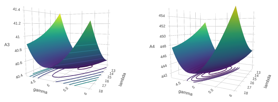
Figure 2: Shapes of the surfaces defined by the functions $A_{3}(\cdot,\cdot)$ and $A_{4}(\cdot,\cdot)$, see Lemma 5.

Remark 1

We displayed in Figure 2 the plots of the function $A_{k}(\cdot,\cdot)$ for $k=3$ and $k=4$. Numerically, we find that the optimal choice for $(\lambda,\gamma)$ is approximately $\lambda=15.89$ and $\gamma=4.4$ for $k=3$ and $\lambda=14.97$ and $\gamma=4.8$ for $k=4$. This leads to the numerical bounds

$$A_{k}\leq\begin{cases}40.40,&k=3,\\ 441.43,&k=4.\end{cases}$$ (182)

These constants are by no means optimal, but we are not aware of any better bound available in the literature. Inequalities of type $\mathbf{E}[\|\boldsymbol{\vartheta}\|_{2}^{k}]\leq A_{k}\mathbf{E}[\|\boldsymbol{\vartheta}\|_{2}^{2}]^{k/2}$ are often referred to as the Kintchine inequality (Khintchine, 1923). According to (Cattiaux and Guillin, 2018), Corollary 4.3 from (Bobkov, 1999) implies that $A_{4}\leq 49$ for one-dimensional $\boldsymbol{\vartheta}$ with log-concave density. Getting such a small constant in the multidimensional case would be of interest for applications to MCMC sampling.

Acknowledgments

This work was partially supported by the grant Investissements d’Avenir (ANR-11-IDEX-0003/Labex Ecodec/ANR-11-LABX-0047).

References

- Baker et al. (2019) J. Baker, P. Fearnhead, E. B. Fox, and C. Nemeth. Control variates for stochastic gradient mcmc. Statistics and Computing, 29(3):599–615, May 2019.
- Bernton (2018) E. Bernton. Langevin Monte-Carlo and JKO splitting. In Conference On Learning Theory, COLT 2018, Stockholm, Sweden, 6-9 July 2018, volume 75 of Proceedings of Machine Learning Research, pages 1777–1798. PMLR, 2018.
- Bobkov (1999) S. G. Bobkov. Isoperimetric and analytic inequalities for log-concave probability measures. Ann. Probab., 27(4):1903–1921, 1999. ISSN 0091-1798.
- Bolley and Villani (2005) F. Bolley and C. Villani. Weighted csiszár-kullback-pinsker inequalities and applications to transportation inequalities. Annales de la Faculté des sciences de Toulouse : Mathématiques, Ser. 6, 14(3):331–352, 2005.
- Borwein et al. (2009) J. M. Borwein, O. Chan, et al. Uniform bounds for the complementary incomplete gamma function. Mathematical Inequalities and Applications, 12:115–121, 2009.
- Brascamp and Lieb (1976) H. J. Brascamp and E. H. Lieb. On extensions of the brunn-minkowski and prékopa-leindler theorems, including inequalities for log concave functions, and with an application to the diffusion equation. Journal of Functional Analysis, 22(4):366 – 389, 1976.
- Bubeck (2015) S. Bubeck. Convex optimization: Algorithms and complexity. Foundations and Trends in Machine Learning, 8(3-4):231–357, 2015.
- Bubeck et al. (2018) S. Bubeck, R. Eldan, and J. Lehec. Sampling from a log-concave distribution with projected Langevin Monte-Carlo. Discrete & Computational Geometry, 59(4):757–783, Jun 2018.
- Cattiaux and Guillin (2018) P. Cattiaux and A. Guillin. On the Poincaré constant of log-concave measures. arXiv preprint arXiv:1810.08369, 2018.
- Chatterji et al. (2018) N. Chatterji, N. Flammarion, Y. Ma, P. Bartlett, and M. Jordan. On the theory of variance reduction for stochastic gradient Monte-Carlo. In International Conference on Machine Learning, pages 764–773. PMLR, 2018.
- Chen et al. (2020) Y. Chen, R. Dwivedi, M. J. Wainwright, and B. Yu. Fast mixing of Metropolized Hamiltonian Monte-Carlo: Benefits of multi-step gradients. J. Mach. Learn. Res., 21:92:1–92:72, 2020.
- Chen and Vempala (2019) Z. Chen and S. S. Vempala. Optimal convergence rate of Hamiltonian Monte-Carlo for strongly logconcave distributions. CoRR, abs/1905.02313, 2019.
- Cheng and Bartlett (2018) X. Cheng and P. Bartlett. Convergence of Langevin MCMC in KL-divergence. In Proceedings of ALT2018, 2018. URL http://proceedings.mlr.press/v83/cheng18a.html.
- Cheng et al. (2018a) X. Cheng, N. S. Chatterji, Y. Abbasi-Yadkori, P. L. Bartlett, and M. I. Jordan. Sharp convergence rates for Langevin dynamics in the nonconvex setting. CoRR, abs/1805.01648, 2018a.
- Cheng et al. (2018b) X. Cheng, N. S. Chatterji, P. L. Bartlett, and M. I. Jordan. Underdamped Langevin MCMC: A non-asymptotic analysis. In Conference on Learning Theory, pages 300–323. PMLR, 2018b.
- Dalalyan (2017a) A. Dalalyan. Further and stronger analogy between sampling and optimization: Langevin Monte-Carlo and gradient descent. In S. Kale and O. Shamir, editors, Proceedings of the 2017 Conference on Learning Theory, volume 65 of Proceedings of Machine Learning Research, pages 678–689, 07–10 Jul 2017a.
- Dalalyan (2017b) A. S. Dalalyan. Theoretical guarantees for approximate sampling from a smooth and log-concave density. J. R. Stat. Soc. B, 79:651 – 676, 2017b.
- Dalalyan and Karagulyan (2019) A. S. Dalalyan and A. Karagulyan. User-friendly guarantees for the Langevin Monte-Carlo with inaccurate gradient. Stochastic Processes and their Applications, 2019.
- Dalalyan and Riou-Durand (2020) A. S. Dalalyan and L. Riou-Durand. On sampling from a log-concave density using kinetic Langevin diffusions. Bernoulli, 26(3):1956–1988, 2020.
- Dalalyan and Tsybakov (2009) A. S. Dalalyan and A. B. Tsybakov. Sparse regression learning by aggregation and Langevin Monte-Carlo. In COLT 2009 - The 22nd Conference on Learning Theory, Montreal, June 18-21, 2009, pages 1–10, 2009.
- Douc et al. (2004) R. Douc, E. Moulines, and J. S. Rosenthal. Quantitative bounds on convergence of time-inhomogeneous Markov chains. Ann. Appl. Probab., 14(4):1643–1665, 2004.
- Durmus and Moulines (2017) A. Durmus and E. Moulines. Nonasymptotic convergence analysis for the unadjusted Langevin algorithm. Ann. Appl. Probab., 27(3):1551–1587, 06 2017. doi: 10.1214/16-AAP1238. URL http://dx.doi.org/10.1214/16-AAP1238.
- Durmus and Moulines (2019) A. Durmus and E. Moulines. High-dimensional Bayesian inference via the unadjusted Langevin algorithm. Bernoulli, 25(4A):2854–2882, 11 2019.
- Durmus et al. (2018) A. Durmus, É. Moulines, and M. Pereyra. Efficient Bayesian Computation by Proximal Markov Chain Monte-Carlo: When Langevin Meets Moreau. SIAM Journal on Imaging Sciences, 11(1), 2018. URL https://hal.archives-ouvertes.fr/hal-01267115.
- Durmus et al. (2019) A. Durmus, S. Majewski, and B. Miasojedow. Analysis of Langevin Monte-Carlo via convex optimization. J. Mach. Learn. Res., 20:73–1, 2019.
- Dwivedi et al. (2018) R. Dwivedi, Y. Chen, M. J. Wainwright, and B. Yu. Log-concave sampling: Metropolis-hastings algorithms are fast! In Conference on Learning Theory, pages 793–797. PMLR, 2018.
- Giannopoulos et al. (2014) A. Giannopoulos, S. Brazitikos, P. Valettas, and B.-H. Vritsiou. Geometry of Isotropic Convex Bodies. 05 2014.
- Gozlan and Léonard (2010) N. Gozlan and C. Léonard. Transport inequalities. A survey. Markov Process. Related Fields, 16(4):635–736, 2010.
- Hargé (2004) G. Hargé. A convex/log-concave correlation inequality for gaussian measure and an application to abstract Wiener spaces. Probability theory and related fields, 130(3):415–440, 2004.
- Jain and Kar (2017) P. Jain and P. Kar. Non-convex optimization for machine learning. Foundations and Trends in Machine Learning, 10(3-4):142–336, 2017.
- Khintchine (1923) A. Khintchine. Über dyadische Brüche. Math. Z., 18(1):109–116, 1923.
- Ledoux (2001) M. Ledoux. The concentration of measure phenomenon. Number 89. American Mathematical Soc., 2001.
- Lovász and Vempala (2006) L. Lovász and S. Vempala. Hit-and-run from a corner. SIAM J. Comput., 35(4):985–1005 (electronic), 2006.
- Lovasz and Vempala (2006) L. Lovasz and S. Vempala. Fast algorithms for logconcave functions: Sampling, Rounding, Integration and Optimization. In 47th Annual IEEE Symposium on Foundations of Computer Science (FOCS 2006), 21-24 October 2006, Berkeley, California, USA, Proceedings, pages 57–68, 2006.
- Ma et al. (2019) Y.-A. Ma, N. Chatterji, X. Cheng, N. Flammarion, P. Bartlett, and M. I. Jordan. Is there an analog of Nesterov Acceleration for MCMC? arXiv preprint arXiv:1902.00996, 2019.
- Majka et al. (2020) M. B. Majka, A. Mijatović, and Łukasz Szpruch. Nonasymptotic bounds for sampling algorithms without log-concavity. The Annals of Applied Probability, 30(4):1534 – 1581, 2020.
- Mangoubi and Smith (2017) O. Mangoubi and A. Smith. Rapid mixing of Hamiltonian Monte-Carlo on strongly log-concave distributions. arXiv preprint arXiv:1708.07114, 2017.
- Mangoubi and Smith (2019) O. Mangoubi and A. Smith. Mixing of Hamiltonian Monte-Carlo on strongly log-concave distributions 2: Numerical integrators. In The 22nd International Conference on Artificial Intelligence and Statistics, pages 586–595, 2019.
- Mangoubi and Vishnoi (2019) O. Mangoubi and N. K. Vishnoi. Nonconvex sampling with the metropolis-adjusted Langevin algorithm. pages 2259–2293, 2019.
- Natalini and Palumbo (2000) P. Natalini and B. Palumbo. Inequalities for the incomplete gamma function. Math. Inequal. Appl, 3(1):69–77, 2000.
- Nelson (1967) E. Nelson. Dynamical Theories of Brownian Motion. Department of Mathematics. Princeton University, 1967.
- Pavliotis (2014) G. A. Pavliotis. Stochastic processes and applications, volume 60 of Texts in Applied Mathematics. Springer, New York, 2014. Diffusion processes, the Fokker-Planck and Langevin equations.
- Qi et al. (2012) F. Qi, Q.-M. Luo, et al. Bounds for the ratio of two gamma functions—from Wendel’s and related inequalities to logarithmically completely monotonic functions. Banach Journal of Mathematical Analysis, 6(2):132–158, 2012.
- Raginsky et al. (2017) M. Raginsky, A. Rakhlin, and M. Telgarsky. Non-convex learning via stochastic gradient Langevin dynamics: a nonasymptotic analysis. In S. Kale and O. Shamir, editors, Proceedings of the 2017 Conference on Learning Theory, volume 65 of Proceedings of Machine Learning Research, pages 1674–1703, 07–10 Jul 2017.
- Roberts and Rosenthal (1998) G. O. Roberts and J. S. Rosenthal. Optimal scaling of discrete approximations to Langevin diffusions. J. R. Stat. Soc. Ser. B Stat. Methodol., 60(1):255–268, 1998.
- Roberts and Stramer (2002) G. O. Roberts and O. Stramer. Langevin diffusions and Metropolis-Hastings algorithms. Methodol. Comput. Appl. Probab., 4(4):337–357 (2003), 2002.
- Roberts and Tweedie (1996) G. O. Roberts and R. L. Tweedie. Exponential convergence of Langevin distributions and their discrete approximations. Bernoulli, 2(4):341–363, 1996.
- Tat Lee et al. (2018) Y. Tat Lee, Z. Song, and S. S. Vempala. Algorithmic Theory of ODEs and Sampling from Well-conditioned Logconcave Densities. arXiv e-prints, art. arXiv:1812.06243, Dec 2018.
- Villani (2008) C. Villani. Optimal transport: old and new, volume 338. Springer Science & Business Media, 2008.
- Wibisono (2018) A. Wibisono. Sampling as optimization in the space of measures: The Langevin dynamics as a composite optimization problem. In Proceedings of the 31st Conference On Learning Theory, volume 75 of Proceedings of Machine Learning Research, pages 2093–3027. PMLR, 06–09 Jul 2018.
- Zou et al. (2019) D. Zou, P. Xu, and Q. Gu. Sampling from non-log-concave distributions via variance-reduced gradient Langevin dynamics. In AISTATS 2019, 16-18 April 2019, Naha, Okinawa, Japan, pages 2936–2945, 2019.