Robust Clustering Using Tau-Scales

Abstract

K means is a popular non-parametric clustering procedure introduced by Steinhaus, (1956) and further developed by MacQueen, (1967). It is known, however, that K means does not perform well in the presence of outliers. Cuesta-Albertos et al (1997) introduced a robust alternative, trimmed K means, which can be tuned to be robust or efficient, but cannot achieve these two properties simultaneously in an adaptive way. To overcome this limitation we propose a new robust clustering procedure called K Tau Centers, which is based on the concept of Tau scale introduced by Yohai and Zamar, (1988). We show that K Tau Centers performs well in extensive simulation studies and real data examples. We also show that the centers found by the proposed method are consistent estimators of the “true” centers defined as the minimizers of the the objective function at the population level.

1 Introduction

Clustering is a useful tool in unsupervised data analysis. Several $p$-dimensional measurements, $\mathbf{x}_{1},\mathbf{...,x}_{n},$ are made on $n$ items and used to find a number, $K$, of homogeneous groups called clusters.

One way to define the clusters is by giving the centers of the clusters. Suppose that the centers of the clusters $\boldsymbol{\mu}_{1},...\boldsymbol{\mu}_{K}$ are given, where each center is an element of $\mathbb{R}^{p}.$ Then the clusters $C_{k},$ $1\leq k\leq K$ can be defined by

$$C_{k}=\{\mathbf{x}_{i}:\min_{1\leq j\leq K}||\mathbf{x}_{i}-\boldsymbol{\mu}_{j}||=||\mathbf{x}_{i}-\boldsymbol{\mu}_{k}||\},$$ (1)

where $\|\cdot\|$ is the Euclidean norm. In this paper we consider the robust estimation of the cluster centers.

There are many parametric and nonparametric approaches for clustering. One of the most popular non-parametric procedures is K means, introduced by Steinhaus, (1956), and popularized MacQueen, (1967). K means optimizes a very natural objective function and therefore is conceptually simple and appealing. Moreover, K means has been efficiently implemented in statistical software.

The K means clustering procedure can be described as follows. Let

$$D(\mathbf{x}_{i,}\boldsymbol{\mu}_{1},...\boldsymbol{\mu}_{K})=\min_{1\leq j\leq K}||\mathbf{x}_{i}-\boldsymbol{\mu}_{j}||,1\leq i\leq n$$

Then the centers of the clusters are obtained by

$$(\widehat{\boldsymbol{\mu}}_{1},...\widehat{\boldsymbol{\mu}}_{K})=\arg\min_{\boldsymbol{\mu}_{1},...\boldsymbol{\mu}_{K}}\sum_{i=1}^{n}D^{2}(\mathbf{x}_{i,}\boldsymbol{\mu}_{1},...\boldsymbol{\mu}_{K})$$

Unfortunately K-means is very sensitive to the presence of outliers, defined as points that lay far away from all the clusters. To illustrate this point, in Figure 1 (A) we show two clusters generated by two bivariate normal distributions. The K-mean cluster centers, marked as triangles, are well identified in panel (A). In panel (B) we add 10% percent of outliers and observe that the K-means cluster centers are no longer well identified.

Procedures that are not much affected by the presence of outliers are called robust. Cuesta-Albertos et al., (1997) noted that K-means is not robust and proposed a robust alternative, called trimmed K-means (TK-means).This procedure find the centers as K-means after eliminating a fraction $\alpha$ of the observations. The trimmed points are iteratively defined as those further away from the current cluster centers. K-means is then applied to the remaining points. When the trimming constant $\alpha$ is well specified, the outliers are likely identified and trimmed. However, in practice $\alpha$ is unknown and difficult to estimate.

(A)	(B)

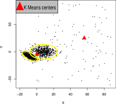
Figure 1: K means applied to data before (A) and after (B) 10% of outliers are added to the sample

The rest of the paper is organized as follows. In Section 2 we define the K-Tau-Centers clustering procedure (K-Tau) and give an algorithm to compute it. In Section 3 we establish the consistency of the estimator. That is, we show that the estimated cluster centers approach the population cluster centers defined as the solution of K-Tau at the population level. In Section 4 we conduct a simulation study to compare K Tau with K means and TK means. In Section 5 we apply K-Tau to the processing of satellite images and illustrate the possible application of robust clustering procedures to the search of missing objects. In Appendix I we derive the estimating equation of K-Tau. In Appendix II we prove the strong consistency of this procedure.

2 K-Tau-Centers

Scale estimators play a central role in the definition of our procedure and therefore they are briefly reviewed in the next section.

2.1 Scale estimators

Given a sample $u_{1},...,u_{n}$ of real numbers, a scale estimator $s(u_{1},...,u_{n})$ is a measure of how large in absolute value are the elements of a sample. An scale estimator should have the following properties: (1) $s(u_{1},...,u_{n})$ only depend on $|u_{1}|,...,|u_{n}|$; (2) $s(0,...,0)=0$; (3) $|v_{1}|\geq|u_{1}|,...,|v_{n}|\geq|u_{n}|$ implies that $s(v_{1},...,v_{n})\geq s(u_{1},...,u_{n})$; (4) $s(\lambda u_{1},...,\lambda u_{n})=|\lambda|s(u_{1},...,u_{n})$; (5) $s(u_{i_{1}},...,u_{i_{n}})=s(u_{1},...,u_{n})$ for any permutation $i_{1},...,i_{n}$. The following are examples of scale estimators:

1) L₂ scale $s_{2}(u_{1},...,u_{n})=\left({\sum_{i=1}^{n}}u_{i}^{2}/n\right)^{1/2}$

2) L₁ scale $s_{1}(u_{1},...,u_{n})=(1/n){\sum\limits_{i=1}^{n}}|u_{i}|$

3) $\alpha$-trimmed scale $s_{\alpha}(u_{1},...,u_{n})=\sum_{i\leq n(1-\alpha)}|u_{(i)}|/[n(1-\alpha)]$

4) Median scale $s_{\text{med}}(u_{1},...,u_{n})=$median$(|u_{1}|,...,|u_{n}|)$

5) M scale, Huber (1964). The value $s_{\text{M}}(u_{1},...,u_{n})$ is implicitly defined by a value $s$ that solves

$$\frac{1}{n}{\displaystyle\sum}_{i=1}^{n}\rho\left({u_{i}}/{s}\right)=b$$ (2)

where $\rho:\mathbb{R}\rightarrow\mathbb{R}_{\geq 0}$ is even, non decreasing in the absolute value and bounded. Usually $b=\max\rho/2$  for breakdown point equal to $1/2$. The breakdown point is a measure of the robustness of an estimator. It is the minimum fraction of outliers that may take the value of the estimator to the boundary of the parameter space. In the case of a scale estimator the extremes cases are infinite and zero. The function $\rho$ may be for example a a member of the bi-square family given by

$$\rho_{{}_{T}}(u,c)=1-\left(1-\left({u}/{c}\right)^{2}\right)^{3}I(|u|\leq c).$$

6) Tau scale, Yohai and Zamar, (1988). These scale estimators combine high Gaussian efficiency and high breakdown point. This is an advantage over M scales which cannot achieve these two properties simultaneously. To define a $\tau$ scale we need two functions, $\rho_{1}$ and $\rho_{2}$ satisfying the conditions specified in the definition of M scales. Given a sample $u_{1},...,u_{n}$, we first compute an M scale $s=s(u_{1},...,u_{n})$ using $\rho_{1}$. The $\tau$ scale is then defined as

$$s_{\tau}(u_{1},...,u_{n})=\left(\sum_{i=1}^{n}\rho_{2}\left({u_{i}}/{s}\right)/n\right)s.$$

The first two scales are not robust because a single observation can make them arbitrarily large. Scales 3-5 can achieve high breakdown point and high efficiency (but not both properties together). The tau scale can be tuned to achieve robustness and efficiency simultaneously.

2.2 K-Tau clustering

First we observe that K means can be formulated as a scale minimization problem. In fact, the K means cluster centers are given by

$$(\widehat{\boldsymbol{\mu}}_{1},...\widehat{\boldsymbol{\mu}}_{K})=\arg\min_{\boldsymbol{\mu}_{1},...\boldsymbol{\mu}_{K}}s_{2}(D(\mathbf{x}_{1},\boldsymbol{\mu}_{1},...,\boldsymbol{\mu}_{K}),...,D(\mathbf{x}_{n},\boldsymbol{\mu}_{1},...,\boldsymbol{\mu}_{K})).$$

It is clear from this formulation that the lack of robustness of K means derives from the lack of robustness of $s_{2}$. Following this reasoning, we define a robust and efficient clustering procedure by replacing $s_{2}$ by $s_{\tau}.$ The cluster centers are now defined as:

$$(\widetilde{\boldsymbol{\mu}}_{1},...\widetilde{\boldsymbol{\mu}}_{K})=\arg\min_{\boldsymbol{\mu}_{1},...\boldsymbol{\mu}_{K}}s_{\tau}(D(\mathbf{x}_{1},\boldsymbol{\mu}_{1},...,\boldsymbol{\mu}_{K}),...,D(\mathbf{x}_{n},\boldsymbol{\mu}_{1},...,\boldsymbol{\mu}_{K}))$$

The corresponding cluster partition $\{C_{1},C_{2},...,C_{K}\}$ is given by equation (1) with $\boldsymbol{\mu}_{k}=\widetilde{\boldsymbol{\mu}}_{k},$ $\ 1\leq k\leq K.$

2.3 Estimating equations

In the case of K means, the clusters centers that minimize $s_{2}$ are simply the mean of each group. On the other hand, the cluster centers corresponding to K-TAU satisfy the following fixed point equations

$$\boldsymbol{\mu}_{k}=\frac{\sum_{i\in C_{k}}w\left({\|\mathbf{x}_{i}-\boldsymbol{\mu}_{k}\|}/{s}\right)\mathbf{x}_{i}}{\sum_{i\in C_{k}}w\left({\|\mathbf{x}_{i}-\boldsymbol{\mu}_{k}\|}/{s}\right)}\quad 1\leq k\leq K,$$ (3)

where the weight function $w$ is defined as

$$w(t)=A\frac{\psi_{1}(t)}{t}+B\frac{\psi_{2}(t)}{t},$$ (4)

with $\psi_{i}=\rho_{i}^{\prime},$ $i=1,2,$ and $A$ and $B$ are data dependent, namely

$$A=\sum_{i=1}^{n}\left[2\rho_{2}\left(d_{i}/{s}\right)-\psi_{2}\left(d_{i}/s\right)(d_{i}/s)\right]$$ (5)

$$B=\ \sum_{i=1}^{n}\psi_{1}\left(d_{i}/{s}\right)(d_{i}/{s}),\$$ (6)

where $d_{i}={D(\mathbf{x}_{i},\boldsymbol{\mu}_{1},...,\boldsymbol{\mu}_{K})}$, and $s$ is the M-scale of all the distances from each observation to the center of its cluster, that is

$$\frac{1}{n}\sum_{i=1}^{n}\rho_{1}\left({D(\mathbf{x}_{i},\boldsymbol{\mu}_{1},...,\boldsymbol{\mu}_{K})}/{s}\right)=b.$$ (7)

The Appendix I contains the derivation of these estimating equations.

2.4 Computing algorithm

The estimating equations given above suggest the following iterative algorithm to compute the cluster centers.

Initialization Step: $K$ random points (or otherwise selected points) are needed to start the iterations.

Updating Step: Suppose that centers $\boldsymbol{\mu}_{1}^{(l)},\dots,\boldsymbol{\mu}_{K}^{(l)}$ are given. Let $C_{1}^{(l)},...,C_{K}^{(l)}$ be the corresponding clusters. First, we compute the M scale $s^{(l+1)}$ by solving

$$\frac{1}{n}\sum_{i=1}^{n}\rho_{1}\left({D(\mathbf{x}_{i},\boldsymbol{\mu}_{1}^{(l)},...,\boldsymbol{\mu}_{K}^{(l)})}/{s}\right)=0.5.$$

Next, the constants $A^{(l+1)}$, $B^{(l+1)}$ are computed using equations (5) and (6), replacing $(\boldsymbol{\mu}_{1},...,\boldsymbol{\mu}_{K})$ and $s$ by $\boldsymbol{\mu}_{1}^{(l+1)},...,\boldsymbol{\mu}_{K}^{(l+1)}$ and $s^{(l+1)\text{ }}$ respectively. The new weight function $\ w^{(l+1)}$ is then defined by equation (4) replacing $A$ and $B$ by $A^{(l+1)}$ and $B^{(l+1)}$. Finally, the new centers are given by

$$\boldsymbol{\mu}_{k}^{(l+1)}=\frac{\sum_{i\in C_{k}}w^{(l+1)}\left({\|\mathbf{x}_{i}-\boldsymbol{\mu}_{k}^{(l)}\|}/{s^{(l+1)}}\right)\mathbf{x}_{i}}{\sum_{i\in C_{k}}w^{(l+1)}\left({\|\mathbf{x}_{i}-\boldsymbol{\mu}_{k}^{(l)}\|}/{s^{(l+1)}}\right)},1\leq k\leq K.$$

Stopping Rule: Given a prescribed tolerance value $\varepsilon$, the algorithm stops when

$${\left\|\boldsymbol{\mu}_{k}^{(l+1)}-\boldsymbol{\mu}_{k}^{(l)}\right\|}/{\left\|\boldsymbol{\mu}_{k}^{(l)}\right\|}\leq\varepsilon,\ 1\leq k\leq K.$$

Notice that when $\rho_{1}(t)=\rho_{2}(t)=t^{2}$ and $b=1$ we have $s_{\tau}=s_{2}$ and the presented computing algorithm reduces to the classic Lloyd’s K means Algorithm Lloyd, (1982).

Further details: We repeat the above procedure $H$ times with different starting points. One possibility is to choose the initial $K$ centers at random from the observations. There exist more sophisticated ways for obtaining starting points such as the ROBIN algorithm, Al Hasan et al., (2009). This algorithm looks for observations in high density areas that are far from each other. We use ROBIN algorithm once and random starts $(H-1)$ times. Let $\boldsymbol{\mu}_{1}^{h},...,\boldsymbol{\mu}_{k}^{h},..,.\boldsymbol{\mu}_{K}^{h}$, $1\leq h\leq H$ be the cluster centers obtained in the h^th replication. Let

$$h_{0}=\arg\min_{1\leq h\leq H}s_{\tau}(D(\mathbf{x}_{1},\boldsymbol{\mu}_{1}^{h},...,\boldsymbol{\mu}_{K}^{h}),...,D(\mathbf{x}_{n},\boldsymbol{\mu}_{1}^{h},...,\boldsymbol{\mu}_{K}^{h}))$$

The final cluster centers are $(\hat{\boldsymbol{\mu}}_{1},...,\hat{\boldsymbol{\mu}}_{K})=(\boldsymbol{\mu}_{1}^{h_{0}},...,\boldsymbol{\mu}_{K}^{h_{0}})$.

In our implementation we use $\rho_{1}=\rho(t/c_{1})$ and $\rho_{2}=\rho(t/c_{2})$, with $\rho$ equal to the smooth hard-rejection loss function given by

$$\rho(t)\!=\!\left\{\begin{array}[]{lcc}1.38t^{2}&\mbox{ if }&|t|<\frac{2}{3}\\ 0.55\!-\!2.69t^{2}\!+\!10.76t^{4}\!-\!11.66t^{6}+\!4.04t^{8}&\mbox{ if }&\frac{2}{3}\leq|t|\leq 1\\ 1&\mbox{ if}&|t|>1.\end{array}\right.$$ (8)

The constants $c_{1}$ and $c_{2}$ depend on $p$ are such that the tau scale is robust and efficient, following Maronna and Yohai, (2017). The $\rho_{i}$ functions are smooth, quadratic at the center and quickly reach their maximum value of one at $c_{i}$.

Outliers detection: We flag an observation as a potential outlier if it falls outside the region $\mathcal{E}=\cup_{k=1}^{K}\mathcal{E}_{k}$, where $\mathcal{E}_{k}$ is the confidence ellipsoid determined by

$$\mathcal{E}_{k}=\{\mathbf{x}\in\mathbb{R}^{p}:d^{2}(\mathbf{x},\hat{\boldsymbol{\mu}}_{k},\hat{\Sigma}_{k})\leq\chi^{2}_{p,1-\beta}\},$$ (9)

where $d^{2}(\mathbf{x},\boldsymbol{\mu},\Sigma)=(\mathbf{x}-\boldsymbol{\mu})^{t}\Sigma^{-1}(\mathbf{x}-\boldsymbol{\mu})$ is the squared Mahalanobis distance and $(\hat{\boldsymbol{\mu}}_{k},\hat{\Sigma}_{k})$ are robust estimators of location and scatter matrix. We use the generalized S-estimators defined in Agostinelli et al., (2015) and implemented in Leung et al., (2015).

2.5 Improved K-Tau.

We add the following step to account for possibly different cluster shapes and sizes. First, for each cluster $C_{k}$, we compute new S-estimators estimators of location and scatter denoted $\widetilde{\boldsymbol{\mu}}_{k}$ and $\widetilde{\Sigma}_{k}$, respectively, using the package GSE cited before in Section 2.4. Improved clusters are defined as

$$G_{k}=\left\{\mathbf{x}_{i}:\min_{1\leq j\leq K}d(\mathbf{x}_{i},\widetilde{\boldsymbol{\mu}}_{j},\widetilde{\Sigma}_{j})=d(\mathbf{x}_{i},\widetilde{\boldsymbol{\mu}}_{k},\widetilde{\Sigma}_{k})\right\},$$

where $d^{2}(\mathbf{x},\boldsymbol{\mu},\Sigma)$ is the square Mahalanobis distance $(\mathbf{x}-\boldsymbol{\mu})^{T}\Sigma^{-1}(\mathbf{x}-\boldsymbol{\mu})$. Once the new cluster are computed, possible outliers are flagged using the procedure described in Section 2.4.

Example: We use the dataset M5-data from García-Escudero et al., (2008). These data consists of 1800 points generated from three bivariate normals with means and covariance matrices given by

$$\boldsymbol{\mu}_{1} =(0,8),\text{ }\boldsymbol{\mu}_{2}=(8,0),\boldsymbol{\mu}_{3}=(-8,8),\mbox{~{}~{}~{}~{} and}$$

$$\Sigma_{1} =\left(\begin{array}[]{cc}1&0\\ 0&1\end{array}\right),\Sigma_{2}=\left(\begin{array}[]{cc}45&0\\ 0&30\end{array}\right),\Sigma_{3}=\left(\begin{array}[]{cc}15&-10\\ -10&15\end{array}\right).$$

There are also 200 outliers generated from an uniform distribution in a rectangular box around the bulk of data. The regular points are 20% in cluster 1, 40 % in cluster 2 and 40% in cluster 3. Panel A in Figure 2 shows the data with 0.95-level ellipsoid around each cluster. Two of the clusters show some overlap. Panel B shows the true cluster in colors red, green and blue. The outliers are shown in black . The results from K-Tau and improved K-Tau are shown in panel C and D, respectively. Improved K-Tau performs better because the shape of the clusters is far from spherical.

$$\begin{array}[]{ccc}\includegraphics[scale={0.45}]{M5Data1.pdf}&\includegraphics[scale={0.45}]{M5Data2.pdf}&\\ \includegraphics[scale={0.45}]{M5Data3.pdf}&\includegraphics[scale={0.45}]{M5Data4updated.pdf}&\end{array}$$

Figure 2: (A) Data-set “M5”. Yellow solid lines show the $95\%$ confidence ellipsoids for the three clusters. (B) True clusters, with outliers shown in black. (C) Results from K-Tau (D) Results from improved K-Tau.

3 Consistency of K-Tau Centers

Let $\mathbf{x}$ be a random vector in $\mathbb{R}^{p}$ with distribution function $F$ and let $\mathcal{A}=\{\boldsymbol{\mu}_{1},...,\boldsymbol{\mu}_{K}\}$ be a set of $K$ distinct points in $R^{p}$. We define the $M$-scale functional , $S_{M}(F)=S_{M}(F,\mathcal{A})$, as the solution in $s$ of the equation

$$E_{F}\left(\rho_{1}\left(D(\mathbf{x},\mathcal{A})/s\right)\right)=1/2,$$

with $D(\mathbf{x},\mathcal{A})$ defined by

$$D(\mathbf{x},\mathcal{A})=\min_{\boldsymbol{\mu}\mathcal{A}\in}\|\mathbf{x}-\boldsymbol{\mu}\|$$

The corresponding $\tau$-scale functional is

$$S_{\tau}(F,\mathcal{A})=S_{M}(F,\mathcal{A})\left[E\left(\rho_{1}\left(D(\mathbf{x},\mathcal{A})/S_{M}(F,\mathcal{A})\right)\right)\right]^{1/2}.$$

The consistency of K-TAU centers is established the following theorem.

Theorem 1

Let $\mathbf{x}_{1},...,\mathbf{x}_{n}$ be a random sample from $F$ and let $\mathcal{A}_{n}$ be the corresponding set of K-TAU-cluster centers. Suppose that

A1. There exists $a<0.5$ such that the probability of any set of at most $k$ points doesn’t exceed $a$.

A2. There exists a unique $\mathcal{A}_{0}$ such that $\min_{\mathcal{A}}S_{\tau}(F,\mathcal{A})=S_{\tau}(F,\mathcal{A}_{0}).$

Then $\mathcal{A}_{n}\rightarrow^{H}\mathcal{A}_{0}$ a.s., where .$\rightarrow^{H}$ denotes convergence in the Haudorff metric.

Formal definition of Hausdorff metric can be found for example in reference Munkres, (2000), colloquially let $\mathcal{A},\mathcal{B}$ be subsets of $\mathbb{R}^{p}$, if Hausdorff distance between $\mathcal{A}$ and $\mathcal{B}$ is less than $\delta$ then for each $\mathbf{a}\in\mathcal{A}$, there exists $\mathbf{b}=\mathbf{b}(\mathbf{a})\in\mathcal{B}$ satisfying $\|\mathbf{a}-\mathbf{b}\|<\delta$ and reciprocally for each $\mathbf{b}\in\mathcal{B}$ there exists $\mathbf{a}=\mathbf{a}(\mathbf{b})\in\mathcal{A}$ such that $\|\mathbf{b}-\mathbf{a}\|<\delta$. Theorem 1 is proved in the Appendix II.

4 Simulation study

We conducted a simulation study to compare improved K-Tau with K means and trimmed K means. More precisely, the compared procedures are:

K means. The classical K means introduced by Hartigan and Wong, (1979), using the default parameters in the function kmeans from the R package stats.

TK means. The robust TK means introduced by Cuesta-Albertos et al., (1997), using the function tkmeans from the R package tclust by Fritz et al., (2012). The trimming constant $\alpha$ is set to $0.05,0.1,0.2\text{ and }0.3$ and the remaining tuning parameters are set to their default values. Outliers are flagged using the mechanism presented in Section 2.4 with $\beta=0.01$. The confidence ellipsoid $\mathcal{E}_{k}$ has center and scatter matrix given by the classical mean and covariance matrix of the points assigned to the k^th cluster.

IK-Tau.The procedure proposed in Section 2.5 using the function improvedktaucenters in the R package ktaucenters. Outliers are flagged using the mechanism presented in Section 2.4 with $\beta=0.01$. The confidence ellipsoid $\mathcal{E}_{k}$ were obtained by applying the function GSE() from the R package GSE Leung et al., (2015) to each group separately.

Models used in the simulation

Several scenarios, dimension $p=3,5,7,10$ and total number of clusters $K=3,5,7,10$ are considered. Each cluster has size $n_{k}=\theta\min\{p,4\}$, where $\theta$ can take the value 25 or 50 with equal probability.

The observations (for each cluster and replication) are generated from multivariate normal distributions with mean

$$\boldsymbol{\mu}_{k}=\left\{\begin{array}[]{crr}20(-\frac{K}{2}+k)(1,1,1,\dots,1)&&\mbox{ if K is even}\\ &&\\ 20(-\frac{K-1}{2}+k)(1,1,1,\dots,1)&&\mbox{if K is odd},\\ &&\end{array}\right.$$

where $k=1,2,\dots,K$, and covariance matrix $\Sigma_{k}$ generated as follows. First we generate a $p\times p$ matrix $U$ with $U_{ij}\sim\mathcal{U}(-1,1)$ and set ${U}{U}^{t}={P}{\Lambda}{P}^{t}$, where $P$ is orthogonal. Second we create a diagonal matrix $D$ with $D_{ii}\sim\mathcal{U}(1,10)$. Finally we set $\Sigma_{k}={P}{D}{P}^{t}.$

A proportion $\alpha=0.05$ of outliers are added to the sample. The outliers are generated from a uniform distribution on a region obtained as follows. We first expand by a factor of two the smallest box that contains the clean data and then remove the points falling inside the $99\%$ probability ellipsoids of the distributions used to generate the clusters.

Performance measure

Suppose that a clustering procedure is performed on a set of $n$ observations with known cluster membership. To evaluate the performance of the clustering procedure, for each pair of observations $(\mathbf{x}_{i},\mathbf{x}_{j})$ with $1\leq i<j\leq n$ we set $I(i,j)=1$ if observations $\mathbf{x}_{i}$ and $\mathbf{x}_{j}$ are both together or apart in the two partitions. Otherwise, we set $I(i,j)=0$. The Classification Error Rate (CER) is then defined by

$$\text{CER}=1-2\sum_{i<j}I(i,j)/[n(n-1)],$$

which is equal to one minus the Rand index proposed by Rand, (1971). Robust clustering procedures are often used to flag outliers. Hence, in our simulation study we collect the flagged observations in an extra cluster and report the CER performance on the resulting $K+1$ clusters.

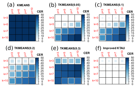
Figure 3: Average Values of CER (multiplied by 1000) from different scenarios. A lighter cell color indicates a better performance.

Simulation results

The results of our extensive simulation study are concisely presented on Figure 3. In each cell a color indicates the average CER value for the scenario identified by the number of clusters $k$ and the dimension $p$. A darker color corresponds to a higher CER value. The color-bar at the right indicates the CER-range values.

Panel (a) in Figure 3 shows that, as expected, K means cannot handle the outliers in the data and gives overall very poor results. Panels (b)-(e) show the results for TK means for different values of the trimming constant $\alpha=0.05,0.10,0.20\text{ and }0.30$. It is clear from these pictures that the best performance of TK means correspond to the “oracle trimming level”  for this method ( $\alpha=0.05$). Table 1 contains the complete numerical results.

$K$	$p$	K means	TK Means				IK-Tau
			$\alpha=0.05$	$\alpha=0.10$	$\alpha=0.20$	$\alpha=0.30$
3	3	224.2	0.7	3.3	10.5	25.4	4.2
3	5	231.0	0.5	2.9	8.5	19.2	4.0
3	7	228.0	0.4	3.3	9.1	18.8	5.6
3	10	228.4	0.3	4.4	11.4	23.2	6.1
5	3	99.8	1.9	4.5	19.7	43.2	1.9
5	5	97.2	8.2	10.3	23.6	44.2	1.6
5	7	97.6	12.5	16.2	26.9	45.3	2.0
5	10	100.9	22.3	24.7	32.5	48.2	3.1
7	3	70.6	28.1	27.1	22.7	42.3	1.1
7	5	69.5	34.4	34.0	28.2	43.4	0.8
7	7	68.9	37.7	38.1	32.8	44.8	0.9
7	10	73.4	42.3	44.7	37.8	46.6	1.1
10	3	52.4	32.1	29.6	29.0	43.1	0.6
10	5	50.9	41.9	37.6	35.8	38.5	0.6
10	7	53.0	46.5	42.1	38.6	34.9	0.6
10	10	52.4	50.9	46.7	41.2	38.9	0.6

Table 1: Simulation results (1000$\times$CER) for the considered clustering procedures.

5 Application

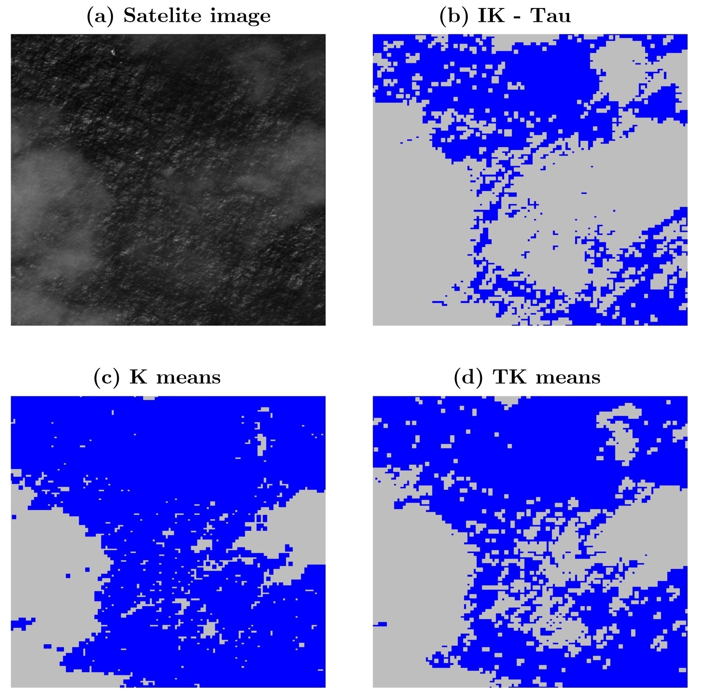
Figure 4: Panel (a) gives the riginal Image. Panels (b), (c) and (d) show the image segmentation produced by K means, TK means and IK-Tau. The 10000 square cells are colored blue or gray according to their assignment to the water or the clouds clusters, respectively.

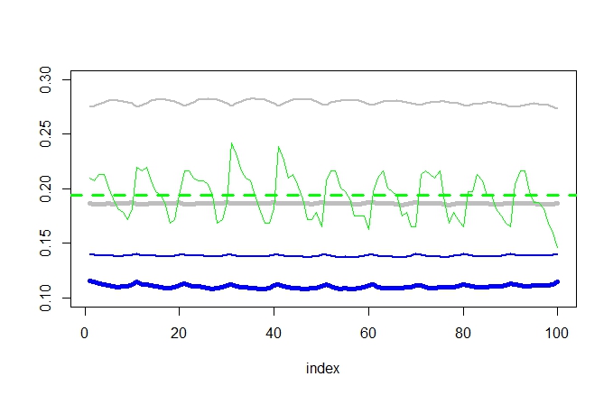
Figure 5: Output Clusters Centers for IK-Tau (Wide line) and K means (Narrow Line). Colors blue and gray correspond to the water and the cloud cluster centers, respectively. A ramdomly selected observation from a low cloud part of the image is shown in green. The constant green line gives the median value for this observation.

Application 1: Cluster analysis of a satellite image

Automatic unsupervised segmentation of satellite images is an important problem in computer vision and automatic anomaly detection. We analyze a satellite image covering $500m^{2}$ of the ocean (image provided by INFOSAT). Each pixel conveys a gray-level intensity scaled between zero and one. Naturally, the image mostly consists of two components: clouds and water. For the analysis, the high resolution image ($1$ pixel $=0.02m^{2}$) is divided into 10000 cells, each packing $10\times 10$ pixels. Hence, our dataset consists of 10000 points in the one–hundred dimensional space $[0,1]^{100}$. Our goal is to segment the image into two clusters (the cloud–cluster and the water–cluster) using IK-Tau. For comparison purposes we also apply K Means and TK means. Figure 4 shows the original image and some clustering results. Blue–colored cells correspond to water and gray–colored cells correspond to clouds.

The high altitude clouds (the brightest areas in the image) are well recognized by all the considered procedures. On the other hand, due to its lack of robustness, K means has difficulty segmenting the low–clouds areas which bear relatively low gray-level intensities. This problem is mainly caused by the presence of a patch of very high altitude clouds with a very high gray–level intensity level. These outliers brings up the intensity level of the K means clouds–cluster center. Figure 5 plots the index versus the gray–level intensity for the clusters centers of K means, K-TAU, and a randomly chosen low–cloud observation. The thick lines correspond to K-TAU, and the thin lines correspond to K means. Low intensity clouds (a randomly chosen low cloud is depicted by the green thick line in Figure 5 lie closer to the K means water–cluster center and get mistakenly assigned to the water–cluster. On the other hand, the considered robust method are not affected by the outliers and are capable to correctly segment the very low clouds.

Application 2: Cluster analysis of high resolution picture

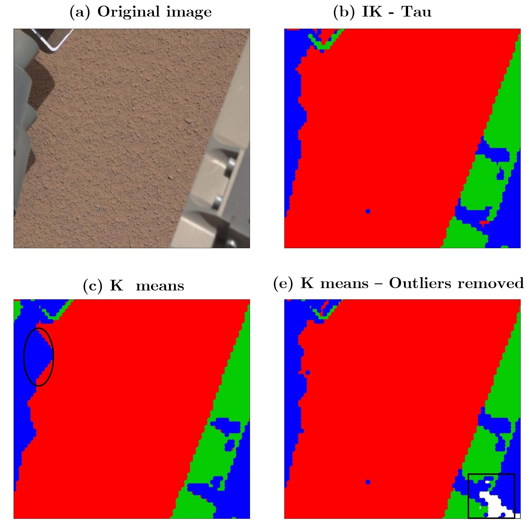
Figure 6: Original Image (panel (a)) and segmentation results obtained from IK-Tau, K means and Kmeans after removing outliers (panels (b), (c) and (d)). Square cells are colored red, green or blue according to their assignment to the SND, SHM or OPM clusters. The black circle in panel (c) pinpoints the sand shadow region in the original image. The blank area in panel (d) are to the removed outlying cells.

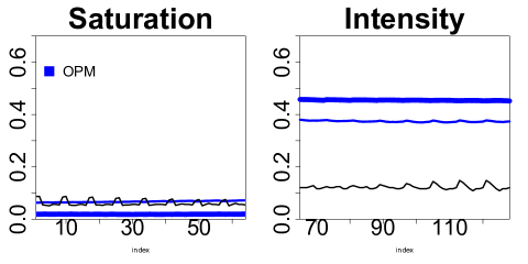
Figure 7: The Opaque Metal cluster Centers corresponding from the improved K-TAU (Wide line) and K means (Narrow Line). An outlying observation is depicted by the thin black line.

In this application we consider is a high resolution colored picture of $495\times 664$ pixels covering an area of $4.0\times 7.5$ $cm^{2}$, provided by NASA NASA, (2016) and displayed in Figure 6 (a). This image was taken by the NASA’s Mars rover Curiosity, and shows the sand soil and metal from the Mars rover itself. Each pixel has assigned three numbers representing the intensity levels of the R, G and B channels, scaled between $0$ and $1$. For example $(0,0,0)$ represents black, $(1,1,1)$ white, $(0,1,0)$ green, etc. Because the $(R,G,B)$ variables are usually highly correlated, a common practice in image segmentation is to transform the $(R,G,B)$ values into the saturation (S) and intensity (I) values, where $I=(R+G+B)/3$ and $S=1-\min(R,G,B)/I$ with $S=0$ when $I=0$. See Chen et al, 2001 Cheng et al., (2001), for further details.

The pixels in the original image are arranged into $8\times 8$ square cells. Since, each pixel has two numbers $(S,I)$, each cell (observation) represents a point in in the one hundred and twenty eight dimensional space $[0,1]^{128}$. Our objective is to segment the image into three clusters, namely the shinning metal (SHM), the opaque metal (OPM) and the sand (SND) clusters. As in the previous application, we use the three clustering algorithms: K means, TK means and IK-Tau with $K=3$. Since the two robust procedures give similar results, only those of IK-Tau are displayed in Figure 6. The nonrobust K means is affected by the presence a small fraction of very dark metal cells in the lower right corner of Figure 6 (a). As shown in Figure 7, the dark metal cells have very low I level, and very high S level. These outliers bring up the S level and down the I level of the OPM cluster center in the case of K means. We notice that the outliers represent $1.5\%$ of the image and $15\%$ of the OPM cluster. As a consequence the shaded sand region enclosed by the ellipse in Figure 6 (c) are incorrectly assigned to the OPM cluster by K means. To validate this reasoning we recompute the K means clusters after removing the aforementioned outliers (the cells delimited by the rectangle in the lower right corner of panel (d) of Figure 6). Now the K means results are consistent with those of the robust clustering procedures.

Searching for lost objects

We now show examples of how large image data in conjunction with robust cluster analysis could be used in computer-aided searches for lost objects. Our first example continues from Application 1. In this case, the lost object is the Tunante II, a 12.5 meter-long yacht with four crew on board lost during a storm off the coast of Brazil. Note that the boat is made of a material mostly absent in the satellite image. Our second example continues from Application 2 and the lost object is a small metal screw detached from the Curiosity Rover, during its exploration of Mars. In this case the lost object is made of a material (metal) well represented in the image making its automatic finding more difficult.

Looking for the lost boat

Naturally we hope that the small yacht reflects the signal differently from the water and clouds in the image. Therefore, the cells containing the boat should appear as outliers in the clustering results. The cell size in Application 1 has been intendedly chosen so that the boat is fully contained by at most four neighboring cells. Using the results from Application 1, we identify the most extreme outlier, that is, the cell lying further away from its cluster center (see Figure 9). Proceeding in this way, all the considered robust and nonrobust cluster algorithms succeed in locating the yacht Tunante.

Searching for the lost screw

In this example we search for a small screw detached form the land rove Mars, using the cluster results from Application 2. The screw is made of a material – metal – that makes up $25\%$ of the image. The image data consists of an $n\times p$ data matrix $X$ with $n=5063$ rows ( each row corresponding to a cell of $8\times 8$ pixels) and $p=128$ columns (each column corresponding to the saturation and the intensity values for the $64$ pixels in each cell). The clustering results from Application 2 yielded three clusters of sizes $n_{1}=3918$, $n_{2}=617$ and $n_{3}=528$ corresponding to sand, opaque metal and shinning metal, respectively. Assuming that we know the type of material of the missing object (e.g. a screw made of opaque metal) we can restrict attention to the $n_{2}\times 2$ geographic submatrix that gives the position of the cells assigned to the OPM cluster (see Figure 8). We perform a second robust cluster analysis on these geographic data. Clearly from Figure 8 (a) any isolated outliers from a second robust cluster analysis of this geographic data are candidates for the location of the missing screw. The robust analysis exposes the remarkable isolated point in Figure 8 (a) which indeed corresponds to the missing screw. The non-robust analysis leads to the much less informative Figure 8 (b).

Figure 8: geographic submatrix corresponding to Opaque Metal cluster obtained by (a) K-TAU, (b) K means

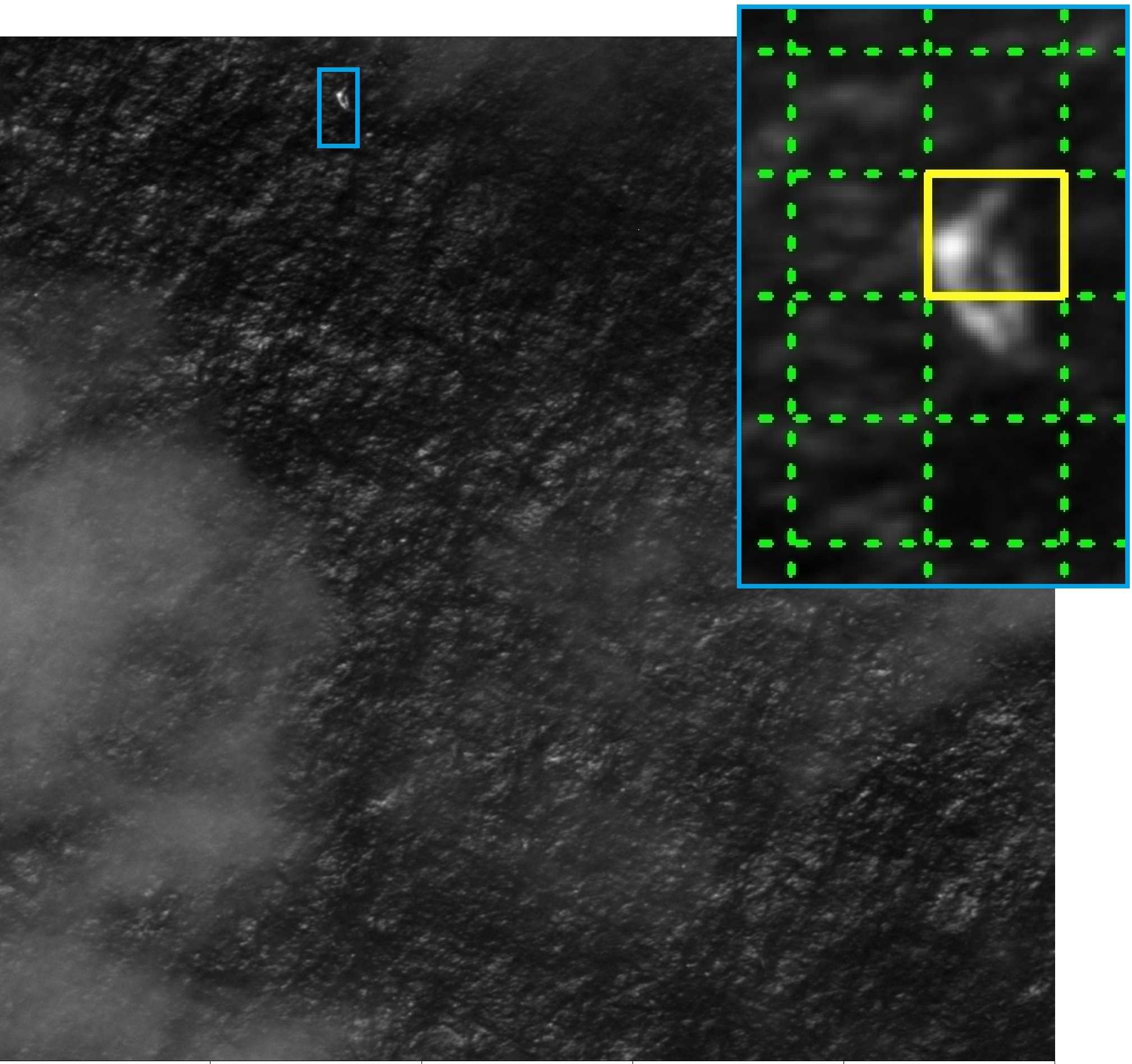
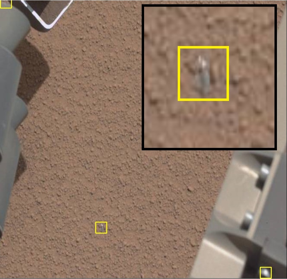
Figure 9: Left: The boat found by the algorithm. Square cells of size $10\times 10$ are shown in green dotted lines, the observation found is in yellow. Right: The screw found by the 2-step procedure. The candidates are indicated in yellow squares on the left upper corner, right lower corner, and in the middle, the region of the screw is expanded in the black rectangle.

Appendix I: Derivation of Estimating equations

Notation

We establish the notation as follows

$$\boldsymbol{\mu}=(\boldsymbol{\mu}_{1},\boldsymbol{\mu}_{2},\dots,\boldsymbol{\mu}_{K}),\mbox{where }\boldsymbol{\mu}_{k}\in\mathbb{R}^{p},$$

$$\boldsymbol{d}(\boldsymbol{\mu})=(d_{1}(\boldsymbol{\mu}),d_{2}(\boldsymbol{\mu}),\dots,d_{n}(\boldsymbol{\mu})),\quad\mbox{where }\quad d_{i}(\boldsymbol{\mu})=\min_{1\leq k\leq K}{\|\mathbf{x}_{i}-\boldsymbol{\mu}_{k}\|},\ \ 1\leq i\leq n.$$

First of all, we set $k$, $1\leq k\leq K$, and compute the derivatives $\partial d_{i}(\boldsymbol{\mu})/\partial\boldsymbol{\mu}_{k}\$ and $\ \partial s(\boldsymbol{d}(\boldsymbol{\mu}))/\partial\boldsymbol{\mu}_{k}\$

• derivation of $\partial d_{i}(\boldsymbol{\mu})/\partial\boldsymbol{\mu}_{k}$

  $$\frac{\partial d_{i}(\boldsymbol{\mu})}{\partial\boldsymbol{\mu}_{k}}=\left\{\begin{array}[]{cc}-\displaystyle\frac{(\mathbf{x}_{i}-\boldsymbol{\mu}_{k})}{||\mathbf{x}_{i}-\boldsymbol{\mu}_{k}||}&\quad\mbox{si }\ \mathbf{x}_{i}\in G_{k}\\ &\\ 0&\quad\mbox{si }\ \mathbf{x}_{i}\notin G_{k}\end{array}\right.$$ (10)

• derivation of $\partial s(\boldsymbol{d}(\boldsymbol{\mu}))/\partial\boldsymbol{\mu}_{k}$

  $s(\boldsymbol{d}(\boldsymbol{\mu}))$, satisfies (2), therefore, by implicit differentiation,

  $$\frac{\partial}{\partial\boldsymbol{\mu}_{k}}\left(\frac{1}{n}\sum_{i=1}^{n}\rho_{1}\left(\frac{d_{i}(\boldsymbol{\mu})}{s(\boldsymbol{d}(\boldsymbol{\mu}))}\right)\right)=0$$

  $$\frac{1}{n}\sum_{i=1}^{n}\psi_{1}\left(\frac{d_{i}(\boldsymbol{\mu})}{s(\boldsymbol{d}(\boldsymbol{\mu}))}\right)\frac{\partial}{\partial\boldsymbol{\mu}_{k}}\left(\frac{d_{i}(\boldsymbol{\mu})}{s(\boldsymbol{d}(\boldsymbol{\mu}))}\right)=0,$$

  this implies

  $$\sum_{i=1}^{n}\psi_{1}\left(\frac{d_{i}(\boldsymbol{\mu})}{s(\boldsymbol{d}(\boldsymbol{\mu}))}\right)\left(\frac{\partial d_{i}(\boldsymbol{\mu})}{\partial\boldsymbol{\mu}_{k}}s(\boldsymbol{d}(\boldsymbol{\mu}))-d_{i}(\boldsymbol{\mu})\frac{\partial s(\boldsymbol{d}(\boldsymbol{\mu}))}{\partial\boldsymbol{\mu}_{k}}\right)=0,$$

  From here, we obtain

  $$\frac{\partial s(\boldsymbol{d}(\boldsymbol{\mu}))}{\partial\boldsymbol{\mu}_{k}}=-\frac{\sum_{i=1}^{n}\psi_{1}\left(\frac{d_{i}(\boldsymbol{\mu})}{s(\boldsymbol{d}(\boldsymbol{\mu}))}\right)\frac{\partial d_{i}(\boldsymbol{\mu})}{\partial\boldsymbol{\mu}_{k}}}{\sum_{i=1}^{n}\psi_{1}\left(\frac{d_{i}(\boldsymbol{\mu})}{s(\boldsymbol{d}(\boldsymbol{\mu}))}\right)\frac{d_{i}(\boldsymbol{\mu})}{s(\boldsymbol{d}(\boldsymbol{\mu}))}}$$

  Let $B(\boldsymbol{\mu})$ be a real number depending on $\boldsymbol{\mu}$

  $$B(\boldsymbol{\mu})=\frac{1}{n}\sum_{i=1}^{n}\psi_{1}\left(\frac{d_{i}(\boldsymbol{\mu})}{s(\boldsymbol{d}(\boldsymbol{\mu}))}\right)\frac{d_{i}(\boldsymbol{\mu})}{s(\boldsymbol{d}(\boldsymbol{\mu}))}$$

  thus,

  $$\frac{\partial s(\boldsymbol{d}(\boldsymbol{\mu}))}{\partial\boldsymbol{\mu}_{k}}=-\frac{1}{B(\boldsymbol{\mu})}\sum_{i=1}^{n}\psi_{1}\left(\frac{d_{i}(\boldsymbol{\mu})}{s(\boldsymbol{d}(\boldsymbol{\mu}))}\right)\frac{\partial d_{i}(\boldsymbol{\mu})}{\partial\boldsymbol{\mu}_{k}},$$

  by using (10), we get

  $$\frac{\partial s(\boldsymbol{d}(\boldsymbol{\mu}))}{\partial\boldsymbol{\mu}_{k}}=-\frac{1}{B(\boldsymbol{\mu})}\sum_{\mathbf{x}_{i}\in G_{k}}^{n}\psi_{1}\left(\frac{\mathbf{x}_{i}-\boldsymbol{\mu}_{k}}{s(\boldsymbol{d}(\boldsymbol{\mu}))}\right)\frac{(\mathbf{x}_{i}-\boldsymbol{\mu}_{k})}{||\mathbf{x}_{i}-\boldsymbol{\mu}_{k}||}.$$ (11)

Now we find the centers that minimize $J_{\tau}$ given by

$$J_{\tau}^{2}\left(\boldsymbol{\mu}_{1},...,\boldsymbol{\mu}_{K}\right)=s^{2}(\boldsymbol{d}(\boldsymbol{\mu}))\frac{1}{n}\sum_{i=1}^{n}\rho_{2}\left(\frac{d_{i}(\boldsymbol{\mu})}{s(\boldsymbol{d}(\boldsymbol{\mu}))}\right),$$

The estimating equations for the clusters centers are obtained by equating the derivative of $J_{\tau}$ to zero,

$$\frac{\partial}{\partial{\boldsymbol{\mu}_{k}}}\left(J_{\tau}\left(\boldsymbol{\ \mu_{1}},...,\boldsymbol{\mu_{k}}\right)\right)=0,$$

$$\frac{\partial}{\partial{\boldsymbol{\mu}_{k}}}\left(J_{\tau}\left(\boldsymbol{\mu}_{1},...,\boldsymbol{\mu}_{k}\right)\right) = \frac{\partial}{\partial\boldsymbol{\mu}_{k}}\left(s^{2}(\boldsymbol{d}(\boldsymbol{\mu}))\frac{1}{n}\sum_{i=1}^{n}\rho_{2}\left(\frac{d_{i}(\boldsymbol{\mu})}{s(\boldsymbol{d}(\boldsymbol{\mu}))}\right)\right)$$

$$= \frac{\partial s^{2}(\boldsymbol{d}(\boldsymbol{\mu}))}{\partial\boldsymbol{\mu}_{k}}\frac{1}{n}\sum_{i=1}^{n}\rho_{2}\left(\frac{d_{i}(\boldsymbol{\mu})}{s(\boldsymbol{d}(\boldsymbol{\mu}))}\right)+s^{2}(\boldsymbol{d}(\boldsymbol{\mu}))\frac{\partial}{\partial\boldsymbol{\mu}_{k}}\left(\frac{1}{n}\sum_{i=1}^{n}\rho_{2}\left(\frac{d_{i}(\boldsymbol{\mu})}{s(\boldsymbol{d}(\boldsymbol{\mu}))}\right)\right)$$

$$= 2s(\boldsymbol{d}(\boldsymbol{\mu})){\frac{\partial s(\boldsymbol{d}(\boldsymbol{\mu}))}{\partial\boldsymbol{\mu}_{k}}}\frac{1}{n}\sum_{i=1}^{n}\rho_{2}\left(\frac{d_{i}(\boldsymbol{\mu})}{s(\boldsymbol{d}(\boldsymbol{\mu}))}\right)+$$

$$+{s^{2}(\boldsymbol{d}(\boldsymbol{\mu}))}\frac{1}{n}\sum_{i=1}^{n}\psi_{2}\left(\frac{d_{i}(\boldsymbol{\mu})}{s(\boldsymbol{d}(\boldsymbol{\mu}))}\right)\frac{\frac{\partial d_{i}(\boldsymbol{\mu})}{\partial\boldsymbol{\mu}_{k}}s(\boldsymbol{d}(\boldsymbol{\mu}))-d_{i}(\boldsymbol{\mu})\frac{\partial s(\boldsymbol{d}(\boldsymbol{\mu}))}{\partial\boldsymbol{\mu}_{k}}}{{s^{2}(\boldsymbol{d}(\boldsymbol{\mu}))}},$$

grouping $s(\boldsymbol{d}(\boldsymbol{\mu}))\frac{\partial s(\boldsymbol{d}(\boldsymbol{\mu}))}{\partial\boldsymbol{\mu}_{k}}$ from the above equation

$$0=s(\boldsymbol{d}(\boldsymbol{\mu}))\frac{\partial s(\boldsymbol{d}(\boldsymbol{\mu}))}{\partial\boldsymbol{\mu}_{k}}\left\{\frac{1}{n}\sum_{i=1}^{n}2\rho_{2}\left(\frac{d_{i}(\boldsymbol{\mu})}{s(\boldsymbol{d}(\boldsymbol{\mu}))}\right)-\psi_{2}\left(\frac{d_{i}(\boldsymbol{\mu})}{s(\boldsymbol{d}(\boldsymbol{\mu}))}\right)\frac{d_{i}(\boldsymbol{\mu})}{s(\boldsymbol{d}(\boldsymbol{\mu}))}\right\}+$$

$$+\frac{1}{n}\sum_{i=1}^{n}\psi_{2}\left(\frac{d_{i}(\boldsymbol{\mu})}{s(\boldsymbol{d}(\boldsymbol{\mu}))}\right)\frac{\partial d_{i}(\boldsymbol{\mu})}{\partial\boldsymbol{\mu}_{k}}s(\boldsymbol{d}(\boldsymbol{\mu})),$$

defining

$$A(\boldsymbol{\mu})=\frac{1}{n}\sum_{i=1}^{n}2\rho_{2}\left(\frac{d_{i}(\boldsymbol{\mu})}{s(\boldsymbol{d}(\boldsymbol{\mu}))}\right)-\psi_{2}\left(\frac{d_{i}(\boldsymbol{\mu})}{s(\boldsymbol{d}(\boldsymbol{\mu}))}\right)\frac{d_{i}(\boldsymbol{\mu})}{s(\boldsymbol{d}(\boldsymbol{\mu}))},$$

we get

$$0=s(\boldsymbol{d}(\boldsymbol{\mu}))A(\boldsymbol{\mu})\frac{\partial s(\boldsymbol{d}(\boldsymbol{\mu}))}{\partial\boldsymbol{\mu}_{k}}+\frac{1}{n}\sum_{i=1}^{n}\psi_{2}\left(\frac{d_{i}(\boldsymbol{\mu})}{s(\boldsymbol{d}(\boldsymbol{\mu}))}\right)s(\boldsymbol{d}(\boldsymbol{\mu}))\frac{\partial d_{i}(\boldsymbol{\mu})}{\partial\boldsymbol{\mu}_{k}}.$$

By using equations (10), (11), and multiplying by $(-1)$,

$$0=s(\boldsymbol{d}(\boldsymbol{\mu}))\frac{A(\boldsymbol{\mu})}{D(\boldsymbol{\mu})}\sum_{\mathbf{x}_{i}\in G_{k}}\psi_{1}\left(\frac{d_{i}(\boldsymbol{\mu})}{s(\boldsymbol{d}(\boldsymbol{\mu}))}\right)\frac{(\mathbf{x}_{i}-\boldsymbol{\mu}_{k})}{d_{i}(\boldsymbol{\mu})}+$$

$$+\frac{1}{n}\sum_{\mathbf{x}_{i}\in G_{k}}\psi_{2}\left(\frac{d_{i}(\boldsymbol{\mu})}{s(\boldsymbol{d}(\boldsymbol{\mu}))}\right)s(\boldsymbol{d}(\boldsymbol{\mu}))\frac{(\mathbf{x}_{i}-\boldsymbol{\mu}_{k})}{d_{i}(\boldsymbol{\mu})},$$

rearranging,

$$0=\sum_{\mathbf{x}_{i}\in G_{k}}\left[A(\boldsymbol{\mu})\psi_{1}\left(\frac{d_{i}(\boldsymbol{\mu})}{s(\boldsymbol{d}(\boldsymbol{\mu}))}\right)\frac{s(\boldsymbol{d}(\boldsymbol{\mu}))}{d_{i}(\boldsymbol{\mu})}+D(\boldsymbol{\mu})\psi_{2}\left(\frac{d_{i}(\boldsymbol{\mu})}{s(\boldsymbol{d}(\boldsymbol{\mu}))}\right)\frac{s(\boldsymbol{d}(\boldsymbol{\mu}))}{d_{i}(\boldsymbol{\mu})}\right](\mathbf{x}_{i}-\boldsymbol{\mu}_{k}),$$

finally,

$$0=\sum_{\mathbf{x}_{i}\in G_{k}}\left[\frac{A(\boldsymbol{\mu})\psi_{1}\left(t\right)+B(\boldsymbol{\mu})\psi_{2}\left(t\right)}{t}\right]_{t=\frac{d_{i}(\boldsymbol{\mu})}{s(\boldsymbol{d}(\boldsymbol{\mu}))}}(\mathbf{x}_{i}-\boldsymbol{\mu}_{k})$$

From here (3) can be derived easily.

Appendix II: Consistency

Strong consistency for the classic K means was given by Pollard, (1981), while strong consistency for the robust TK means was given by Cuesta-Albertos et al., (1997). Both works prove convergence by showing that the Hausdorff distance ($d_{H}$) between the true centers an the estimated ones tends to zero as the sample size tends to infinity. We provide an analogous result for K-TAU. Our proof uses the results from Lemmas stated and proved in the following section.

Consistency- Lemmas

Lemma 2

Let $\varphi:\boldsymbol{\mathcal{K}_{0}}\to\mathbb{R}$ be a continuous function with a unique minimum $\nu_{0}=\varphi(\mathcal{A}_{0})$, where $\boldsymbol{\mathcal{K}}_{0}=\{\mathcal{A}\subseteq\overline{B},\#\mathcal{A}\leq K\}$, and $\overline{B}$ is a closed ball in $\mathbb{R}^{p}$. Suppose that $(\mathcal{A}_{n})_{n\in\mathbb{N}}\subseteq\boldsymbol{\mathcal{K}_{0}}$ and assume that the following property is satisfied

$$\forall\eta>0\ \exists n_{0}:\varphi(\mathcal{A}_{n})<\eta+\nu_{0}\ \ \ \forall n\geq n_{0},$$

then $d_{H}(\mathcal{A}_{n},\mathcal{A}_{0})\to 0$.

Proof. First of all, we note that $(\boldsymbol{\mathcal{K}_{0}},d_{H})$ is a compact metric space (for a proof we refer for example to Munkres, (2000)). Let $\varepsilon$ be a positive real number, we consider the open ball of radius $\varepsilon$ regarding to Hausdorff distance $\mathcal{B}_{\varepsilon}(\mathcal{A}_{0})$. The set $\boldsymbol{\mathcal{K}}_{1}=\boldsymbol{\mathcal{K}}_{0}\setminus\mathcal{B}_{\varepsilon}(\mathcal{A}_{0})$ is compact. Since $\varphi$ is continuous, it is well defined its minimum over $\boldsymbol{\mathcal{K}}_{1}$, say $\nu_{1}$, namely,

$$\nu_{1}=\min_{\mathcal{A}\in\boldsymbol{\mathcal{K}}_{1}}\varphi(\mathcal{A}),$$

provided $\nu_{0}$ is unique, must be $\nu_{1}>\nu_{0}$, hence we can take $\eta=\nu_{1}-\nu_{0}>0$, the Lemma hypothesis ensures the existence of $n_{0}$, for which, $\forall n\geq n_{0}$

$$\varphi(\mathcal{A}_{n})<(\nu_{1}-\nu_{0})+\nu_{0}=\nu_{1},$$

then $\mathcal{A}_{n}$ can not belong to $\boldsymbol{\mathcal{K}}_{1}$, since in that case it would be less than the minimum. Thus, $\mathcal{A}_{n}\in\mathcal{B}_{\varepsilon}(\mathcal{A}_{0})$   

Lemma 3

Let $\mathcal{A}\subseteq\mathbb{R}^{p}$ be a set of at most $K$ points. We consider $H:[0,+\infty)\rightarrow\mathbb{R}$

$$H(t)=\left\{\begin{array}[]{lrr}1-\mathbb{P}(\mathbf{x}\in\mathcal{A})&\mbox{si }&t=0\\ &&\\ \mathbb{E}\left(\rho(\frac{d(\mathbf{x},\mathcal{A})}{t})\right)&\mbox{si }&t>0\end{array}\right.$$

Then,

1. $H$ is continuous

2. $\lim_{t\rightarrow\infty}H(t)=0$

3. Equation $H(t)=1/2$ has unique solution.

Proof. We will prove 1. First, we see the continuity for $t>0$, set $t_{0}>0$, and take $t_{j}\rightarrow t_{0}$. Let $(f_{j})_{j\in\mathbb{N}}$ be the functions sequence, $f_{j}(\mathbf{x}):=\rho(d(\mathbf{x},\mathcal{A})/t_{j})$, $f_{j}$ are bounded by $1$, and converge pointwise to $\rho({d(\mathbf{x},\mathcal{A})}/{t_{0}})$. Then, by using the Lebesgue dominated convergence Theorem, it is possible to exchange the expectation and the limit in the following equation,

$$\lim_{j\rightarrow\infty}H(t_{j})=\lim_{j\rightarrow\infty}\mathbb{E}\left(\rho\left(\frac{d(\mathbf{x},\mathcal{A})}{t_{j}}\right)\right)=\mathbb{E}\left(\lim_{j\rightarrow\infty}\rho\left(\frac{d(\mathbf{x},\mathcal{A})}{t_{j}}\right)\right)=H(t_{0}).$$

In this way, $H$ is continuous at $t_{0}>0$. Now, it remains to see the continuity at $t=0$, take $t_{j}$ converging decreasingly to $0$,

$$H(t_{j})=\mathbb{E}\left(\rho\left(\frac{d(\mathbf{x},\mathcal{A})}{t_{j}}\right)\right)=\mathbb{E}\left(\rho\left(\frac{d(\mathbf{x},\mathcal{A})}{t_{j}}\right)I_{\{d(\mathbf{x},\mathcal{A})>0\}}\right).$$

For $\rho$- function considered here $\rho(0)=0$, and also if $d(\mathbf{x},\mathcal{A})>0$,

$$\lim_{j\rightarrow\infty}\rho(\frac{d(\mathbf{x},\mathcal{A})}{t_{j}})=\rho(\infty)=1.$$

So, by applying dominated convergence Theorem,

$$\lim_{j\rightarrow\infty}H(t_{j})=\mathbb{E}\left(\lim_{j\rightarrow\infty}\rho\left(\frac{d(\mathbf{x},\mathcal{A})}{t_{j}}\right)I_{\{d(\mathbf{x},\mathcal{A})>0\}}\right)=\mathbb{E}\left(1\cdot I_{\{d(\mathbf{x},\mathcal{A})>0\}}\right)=1-\mathbb{P}(\mathbf{x}\in\mathcal{A}).$$

Thus, $H(t)$ is continuous at $0$.

We will prove 2. Take $t_{j}\rightarrow\infty$, $\rho({d(\mathbf{x},\mathcal{A})}/{t_{j}})\rightarrow 0$ pointwise, thus $H(t_{j})\rightarrow 0$ concluding the proof of 2.

Finally, we will see item 3 of the Lemma, in first place, A.1) Hypothesis implies that $1-\mathbb{P}(\mathbf{x}\in\mathcal{A})>1/2$. We apply the intermediate value Theorem to the function $H(t)$: $H(0)>\frac{1}{2}$, $H(\infty)=0$, then there exists $s$ such that $H(s)=1/2$, proving the existence, to see the uniqueness, suppose that $s_{2}>s_{1}$ are two different solutions, subtracting them,

$$0=H(s_{1})-H(s_{2})=\mathbb{E}\left(\rho\left(\frac{d(\mathbf{x},\mathcal{A})}{s_{1}}\right)-\rho\left(\frac{d(\mathbf{x},\mathcal{A})}{s_{2}}\right)\right).$$

Because $\rho$ is monotonous, the argument inside the expectation is greater or equal than zero, then

$$\mathbb{P}\left(\rho\left(\frac{d(\mathbf{x},\mathcal{A})}{s_{1}}\right)-\rho\left(\frac{d(\mathbf{x},\mathcal{A})}{s_{2}}\right)=0\right)=1,$$ (12)

Thus,

$$\rho\left(\frac{d(\mathbf{x},\mathcal{A})}{s_{1}}\right)=\rho\left(\frac{d(\mathbf{x},\mathcal{A})}{s_{2}}\right)$$

all most everywhere. That may happen in two ways:

• ${d(\mathbf{x},\mathcal{A})}/{s_{1}}={d(\mathbf{x},\mathcal{A})}/{s_{2}}$, but given that $s_{1}\neq s_{2}$, the previous equation only happen if $d(\mathbf{x},\mathcal{A})=0$, that means that $\mathbf{x}\in\mathcal{A}$.

• ${d(\mathbf{x},\mathcal{A})}/{s_{i}}\in[m,+\infty)$, being $m$ the value from which $\rho(x)=1\forall x\geq m$.

Then, we write equation (12) according to the previous two events described, and get

$$\mathbb{P}\left(\mathbf{x}\in\mathcal{A}\right)+\mathbb{P}\left(\frac{d(\mathbf{x},\mathcal{A})}{s_{1}}\in[m,+\infty)\right)=1.$$

from the equation above, and using hypothesis A.1) it turns out $\mathbb{P}\left({d(\mathbf{x},\mathcal{A})}/{s_{1}}\in[m,+\infty)\right)>1/2.$ Finally, we take the $H$ definition and come to a contradiction

$$\frac{1}{2}=H(s_{1})=\mathbb{E}\left(\rho\left(\frac{d(\mathbf{x},\mathcal{A})}{s_{1}}\right)\right)\geq\mathbb{E}\left(\rho\left(\frac{d(\mathbf{x},\mathcal{A})}{s_{1}}\right)I_{\{\frac{d(\mathbf{x},\mathcal{A})}{s_{1}}\in[m,+\infty)\}}\right)$$

$$=\mathbb{P}\left(\frac{d(\mathbf{x},\mathcal{A})}{s_{1}}\in[m,+\infty)\right)>\frac{1}{2}.$$

The absurdity was caused by supposing that there were two different solutions $s_{1}$ and $s_{2}$.   

Lemma 4

Functions $\varphi_{\tau}(\mathcal{A})=\tau(\mathcal{A},F)$ and $\varphi_{M}(\mathcal{A})=M(\mathcal{A},F)$, are continuous regarding to Hausdorff distance.

Proof. Let $\mathcal{A}_{n}$ be a sequence converging to $\mathcal{A}$ in the Hausdorff sense, we will see that $\lim_{n\rightarrow\infty}\varphi_{M}(\mathcal{A}_{n})=\varphi_{M}(\mathcal{A})$. Take $\varepsilon>0$, it is easy to see that for each $\mathbf{x}$, $d(\mathbf{x},\mathcal{A}_{n})\rightarrow d(\mathbf{x},\mathcal{A})$, then, by using dominated convergence Theorem, it turns out that

$$\mathbb{E}\left(\rho_{1}\left(\frac{d(\mathbf{x},\mathcal{A}_{n})}{M(\mathcal{A},F)+\varepsilon}\right)\right)\rightarrow\mathbb{E}\left(\rho_{1}\left(\frac{d(\mathbf{x},\mathcal{A})}{M(\mathcal{A},F)+\varepsilon}\right)\right).$$

On the other hand,

$$\mathbb{E}\left(\rho_{1}\left(\frac{d(\mathbf{x},\mathcal{A})}{M(\mathcal{A},F)+\varepsilon}\right)\right)<\frac{1}{2},$$

then, there exists $n_{0}$ such that $\forall n\geq n_{0}$

$$\mathbb{E}\left(\rho_{1}\left(\frac{d(\mathbf{x},\mathcal{A}_{n})}{M(\mathcal{A},F)+\varepsilon}\right)\right)<\frac{1}{2}.$$ (13)

Analogously it can be shown that exists $n_{1}$, such that $\forall n\geq n_{1}$

$$\mathbb{E}\left(\rho_{1}\left(\frac{d(\mathbf{x},\mathcal{A}_{n})}{M(\mathcal{A},F)-\varepsilon}\right))\right)>\frac{1}{2},$$ (14)

For $n\geq\max\{n_{1},n_{2}\}$, consider the function $H_{n}(t)=\mathbb{E}\left(\rho_{1}(\frac{d(\mathbf{x},\mathcal{A}_{n})}{t})\right)$, we apply Lemma 3, obtaining continuity of $H_{n}(t)$ and uniqueness for the problem

$$\mathbb{E}\left(\rho_{1}\left(\frac{d(\mathbf{x},\mathcal{A}_{n})}{t^{\ast}}\right)\right)=\frac{1}{2}$$

Let $t^{\ast}=M(\mathcal{A}_{n},F)$, through intermediate value theorem for $H_{n}(t)$, inequalities (13) and (14), together with uniqueness shown in 3, it is easy to see that $t^{\ast}\in(M(\mathcal{A},F)-\varepsilon,M(\mathcal{A},F)+\varepsilon)$. Then,

$$|M(\mathcal{A}_{n},F)-M(\mathcal{A},F)|<\varepsilon,$$

thus, $\varphi_{M}(\mathcal{A})=M(\mathcal{A},F)$ is continuous as function of $\mathcal{A}$.

Now, we need to prove the continuity of $\varphi_{\tau}(\mathcal{A})$,

$$\varphi_{\tau}(\mathcal{A})^{2}=(M(A,F))^{2}\mathbb{E}\left(\rho_{2}\left(\frac{d(\mathbf{x},\mathcal{A})}{M(\mathcal{\ A},F)}\right)\right)$$

Take $\mathcal{A}_{n}$ converging to $\mathcal{A}$ in Hausdorff distance, given that $M(\mathcal{A},F)>0$, and $M(\mathcal{A},F)$ is continuous in $\mathcal{A}$, the integrand is continuous and bounded. By using the dominated convergence Theorem we get that $\tau(\mathcal{A}_{n},F)^{2}$ converges to $\tau^{2}(\mathcal{A},F)$. Thus, $\varphi_{\tau}(\mathcal{A})$ is continuous as function of $\mathcal{A}$.   

Lemma 5

(Uncoupled Uniform Convergence over Compact Sets) Consider the set $\boldsymbol{\mathcal{K}}_{0}=\{\mathcal{A}\subseteq\overline{B},\#\mathcal{A}\leq K\}$, where $\overline{B}$ is a closed ball in $\mathbb{R}^{p}$, let $\rho$ be a $\rho$- function and $l_{2}>l_{1}>0$. Let $\mathbf{x}_{1},\mathbf{x}_{2},...,\mathbf{x}_{n}$ independent observations from a random sample of size $n$. Then

$$\lim_{n\rightarrow\infty}\sup_{\mathcal{A}\in\boldsymbol{\mathcal{K}}_{0},s\in[l_{1},l_{2}]}\left|\frac{1}{n}\sum_{i=1}^{n}\rho\left(\frac{d(\mathbf{x}_{i},\mathcal{A})}{s}\right)-E_{F}\left(\rho\left(\frac{d(\mathbf{x},\mathcal{A})}{s}\right)\right)\right|=0\ \ \ \text{a.s.}$$

Proof. We consider the Family

$$\mathcal{G}=\left\{g_{\mathcal{A},s}(\mathbf{x})=\rho\left(\frac{d(\mathbf{x},\mathcal{A})}{s}\right),\mathcal{A}\in\boldsymbol{\mathcal{K}_{0}},s\in[l_{1},l_{2}]\right\}.$$

We want to prove an uniform strong law of large numbers (USLLN) for $\mathcal{G}$. Sufficient conditions for the theorem to hold are given in Pollard, (1984). In particular, it is established that if for each $\varepsilon>0$, there exists a finite family $\mathcal{F}_{\varepsilon}$ satisfying

$$\forall g\in\mathcal{G}\ \ \exists\ \ f_{1},f_{2}\in\mathcal{F}_{\varepsilon},\mbox{ such that }f_{1}\leq g\leq f_{2}\mbox{ and also }\mathbb{E}(f_{2}-f_{1})\leq\varepsilon,$$

then, family $\mathcal{G}$ has a USLLN.

Given $\varepsilon>0$, we show a $\mathcal{F}_{\varepsilon}$ that satisfies this property.

First, because uniform continuity of $\rho$ function, we can choose $\delta>0$ such that

$$|\rho\left(y+\delta\right)-\rho\left(y\right)|<\frac{1}{3}\varepsilon\quad\quad\forall y\in\mathbb{R}$$ (15)

Let $\delta_{1}$ be such that $0<\delta_{1}\leq{l_{1}}\delta$, as $\overline{B}\subseteq\mathbb{R}^{p}$ is a closed ball, it is possible to take a finite subset $\mathcal{J}$ whose elements are $\mathbf{a}_{j}\in\overline{B}$, con $1\leq j\leq N$, $\mathcal{J}=\{\mathbf{a}_{1},\dots,\mathbf{a}_{N}\}$, such that $\forall\mathbf{x}\in\overline{B},\exists j:\|\mathbf{x}-\mathbf{a}_{j}\|<\delta_{1}$. Let $0<\delta_{2}<\varepsilon{l_{1}}/(3C_{\psi})$ be a real number, where $C_{\psi}=\sup_{u\in\mathbb{R}}\psi(u)u$ is a positive number for the $\rho$ function considered here. Consider the partition $[l_{1},l_{2}]=\cup_{i=1}^{M}[s_{i-1},s_{i}]$ with interval length $[s_{i-1},s_{i}]$ less than $\delta_{2}$. Family $\mathcal{F}_{\varepsilon}$ will be

$$\mathcal{F}_{\varepsilon}=\left\{\rho\left(\frac{d(\mathbf{x},\mathcal{A}^{\prime})}{s_{i-1}}\pm\delta\right):\mathcal{A}^{\prime}\subseteq\mathcal{J},\#(A^{\prime})\leq k,1\leq i\leq M\right\}.$$ (16)

Now set an element of $\mathcal{G}$ indexed by $\mathcal{A}$ and $s$, then $s\in[s_{i-1},s_{i}]$, for some $i$, and also there exists a $\mathcal{A}^{\prime}\subseteq\mathcal{J}$, such that $d_{H}(\mathcal{A},\mathcal{A}^{\prime})\leq\delta_{1}.$ Then

$$\frac{d(\mathbf{x},\mathcal{A})}{s}\leq\frac{d(\mathbf{x},\mathcal{A}^{\prime})+\delta_{1}}{s_{i-1}}\leq\frac{d(\mathbf{x},\mathcal{A}^{\prime})}{s_{i-1}}+\frac{\delta_{1}}{l_{1}},$$ (17)

as consequence,

$$\frac{d(\mathbf{x},\mathcal{A})}{s}\geq\frac{d(\mathbf{x},\mathcal{A}^{\prime})-\delta_{1}}{s_{i}}\geq\frac{d(\mathbf{x},\mathcal{A}^{\prime})}{s_{i}}-\frac{\delta_{1}}{l_{2}}\geq\frac{d(\mathbf{x},\mathcal{A}^{\prime})}{s_{i}}-\frac{\delta_{1}}{l_{1}},$$ (18)

Provided $\delta_{1}/l_{1}\leq\delta$, and using the $\rho$ monotonicity at (17) and (18), we get

$$f_{1}(\mathbf{x})\leq\rho\left(\frac{d(\mathbf{x},\mathcal{A})}{s}\right)\leq f_{2}(\mathbf{x}),$$

where

$$f_{1}(\mathbf{x})=\rho\left(\frac{d(\mathbf{x},\mathcal{A}^{\prime})}{s_{i}}-\delta\right),\quad\text{and}\quad f_{2}(\mathbf{x})=\rho\left(\frac{d(\mathbf{x},\mathcal{A}^{\prime})}{s_{i-1}}+\delta\right).$$

It remain to see that choices made on $\delta$, $\delta_{1}$ and $\delta_{2}$ , imply $\mathbb{E}\left(f_{2}-f_{1}\right)\leq\varepsilon$. Indeed,

$$\begin{array}[]{rcl}\mathbb{E}\left(f_{2}-f_{1}\right)&=&\mathbb{E}\left(\rho\left(\frac{d(\mathbf{x},\mathcal{A}^{\prime})}{s_{i}}+\delta\right)-\rho\left(\frac{d(\mathbf{x},\mathcal{A}^{\prime})}{s_{i-1}}-\delta\right)\right)\\ &&\\ &=&\mathbb{E}\left(\rho\left(\frac{d(\mathbf{x},\mathcal{A}^{\prime})}{s_{i}}+\delta\right)-\rho\left(\frac{d(\mathbf{x},\mathcal{A}^{\prime})}{s_{i}}\right)\right)+\mathbb{E}\left(\rho\left(\frac{d(\mathbf{x},\mathcal{A}^{\prime})}{s_{i-1}}\right)-\rho\left(\frac{d(\mathbf{x},\mathcal{A}^{\prime})}{s_{i-1}}-\delta\right)\right)+\\ &&\\ &+&\mathbb{E}\left(\rho\left(\frac{d(\mathbf{x},\mathcal{A}^{\prime})}{s_{i}}\right)-\rho\left(\frac{d(\mathbf{x},\mathcal{A}^{\prime})}{s_{i-1}}\right)\right).\end{array}$$

Applying inequality (15) with $y={d(\mathbf{x},\mathcal{A}^{\prime})}/{s_{i}}$ in their first term, and with $y={d(\mathbf{x},\mathcal{A}^{\prime})}/{s_{i-1}}$ in the second, the absolute value of the first two terms are less than ${2\varepsilon}/{3}$. To bound the last one, by middle value theorem, there exists $\xi_{i}^{\ast}\in[s_{i-1},s_{i}]$ satisfying

$$\rho\left(\frac{d(\mathbf{x},\mathcal{A}^{\prime})}{s_{i}}\right)-\rho\left(\frac{d(\mathbf{x},\mathcal{A}^{\prime})}{s_{i-1}}\right)=-\psi\left(\frac{d(\mathbf{x},\mathcal{A}^{\prime})}{\xi^{\ast}}\right)\frac{d(\mathbf{x},\mathcal{A}^{\prime})}{\xi_{i}^{\ast}}\frac{1}{\xi_{i}^{\ast}}(s_{i}-s_{i-1}).$$

As $\psi(u)u$ is bounded by $C_{\psi}$ it turns out

$$\mathbb{E}\left(\left|\rho\left(\frac{d(\mathbf{x},\mathcal{A}^{\prime})}{s_{i}}\right)-\rho\left(\frac{d(\mathbf{x},\mathcal{A}^{\prime})}{s_{i-1}}\right)\right|\right)\leq\frac{C_{\psi}}{l_{1}}\delta_{2}.$$

Then, as $\delta_{2}$ was chosen in such way that $\delta_{2}\leq{l_{1}\varepsilon}/({3C_{\psi}})$, ${\varepsilon}/{3}$ is a properly bound for the previous term. Thus, we get

$$\mathbb{E}\left(f_{2}-f_{1}\right)\leq\frac{2}{3}\varepsilon+\frac{1}{3}\varepsilon=\varepsilon$$

 

Lemma 6

(Uniform Strong Law of Large Numbers) Consider the set $\boldsymbol{\mathcal{K}}_{0}=\{\mathcal{A}\subseteq\overline{B},\#\mathcal{A}\leq K\}$, where $\overline{B}$ is a closed ball in $\mathbb{R}^{p}$. Suppose A.1) and $(\mathbf{x}_{n})_{n\in\mathbb{N}}$ are $i.i.d^{\prime}s$, then:

$$\lim_{n\rightarrow\infty}\sup_{\mathcal{A}\in\boldsymbol{\mathcal{K}}_{0}}\left|\tau(\mathcal{A},F)-\tau(\mathcal{A},F_{n})\right|=0\ \ \ a.s.$$ (19)

Proof. Consider $h_{1}=\inf_{\mathcal{A}\in\boldsymbol{\mathcal{K}}_{0}}M(\mathcal{A},F)$ and $h_{2}=\sup_{\mathcal{A}\in\boldsymbol{\mathcal{K}}_{0}}M(\mathcal{A},F)$. Take $\varepsilon<{h_{1}}/{2}$. Define $g_{1}$ and $g_{2}$ as follows

$$g_{1}(\mathcal{A})=\mathbb{E}\left(\rho_{1}\left(\frac{d(\mathbf{x},\mathcal{A})}{M(\mathcal{A},F)-\varepsilon}\right)\right)$$ (20)

and

$$g_{2}(\mathcal{A})=\mathbb{E}\left(\rho_{1}\left(\frac{d(\mathbf{x},\mathcal{A})}{M(\mathcal{A},F)+\varepsilon}\right)\right).$$ (21)

As $g_{1}$ and $g_{2}$ are continuous functions regarding to $d_{H}$, and $\boldsymbol{\mathcal{K}}_{0}$ is a compact set under $d_{H}$, minimum and maximum are achieved at $\mathcal{A}_{1}$ and $\mathcal{A}_{2}$ respectively, whose values are $g_{\ell}(\mathcal{A}_{\ell})=d_{\ell},\ell=1,2$. Define $d_{1}$ and $d_{2}$ as $\inf_{\mathcal{A}\in\boldsymbol{\mathcal{K}}_{0}}g_{1}(\mathcal{A})=d_{1}>{1}/{2}$, and $\sup_{\mathcal{A}\in\boldsymbol{\mathcal{K}}_{0}}g_{2}(\mathcal{A})=d_{2}<{1}/{2}$.

Taking a real number $\delta$, $0<\delta\leq(d_{1}-{1}/{2})$ and $0<\delta\leq({1}/{2}-d_{2})$, and through Lemma 5, $\exists\Omega^{\prime},\mathbb{P}(\Omega^{\prime})=1$, satisfying $\forall\omega\in\Omega^{\prime}\exists n_{0}=n_{0}(\omega)$ such that for all $n>n_{0}$

$$\sup_{\mathcal{A}\in\boldsymbol{\mathcal{K}}_{0},s\in[\frac{h_{1}}{2},h_{2}]}\left|\frac{1}{n}\sum_{i=1}^{n}\rho_{1}\left(\frac{d(\mathbf{x}_{i},\mathcal{A})}{s}\right)-\mathbb{E}\left(\rho_{1}\left(\frac{d(\mathbf{x},\mathcal{A})}{s}\right)\right)\right|<\frac{\delta}{2},$$

where $(\mathbf{x}_{i}^{(\omega)})_{i\in\mathbb{N}}$ depends on $\omega$, but we write $(\mathbf{x}_{i})_{i\in\mathbb{N}}$ for short.

Suppose that sequence $\mathcal{A}\in\boldsymbol{\mathcal{K}}_{0}$, then $M(\mathcal{A},F)-\varepsilon\in(h_{1}-\varepsilon,h_{2}-\varepsilon)\subseteq[{h_{1}}/{2},h_{2}]$, thus

$$\sup_{\mathcal{A}\in\boldsymbol{\mathcal{K}}_{0}}\left|\frac{1}{n}\sum_{i=1}^{n}\rho_{1}\left(\frac{d(\mathbf{x}_{i},\mathcal{A})}{M(\mathcal{A},F)-\varepsilon}\right)-\mathbb{E}\left(\rho_{1}\left(\frac{d(\mathbf{x},\mathcal{A})}{M(\mathcal{A},F)-\varepsilon}\right)\right)\right|<\frac{\delta}{2}.$$

Then, the follow inequality is valid for all $\mathcal{A}\in\boldsymbol{\mathcal{K}}_{0}$,

$$\frac{1}{n}\sum_{i=1}^{n}\rho_{1}\left(\frac{d(\mathbf{x}_{i},\mathcal{A})}{M(\mathcal{A},F)-\varepsilon}\right)>\mathbb{E}\left(\rho_{1}\left(\frac{d(\mathbf{x},\mathcal{A})}{M(\mathcal{A},F)-\varepsilon}\right)\right)-\frac{\delta}{2}.$$

So, by taking infimum at the right hand side

$$\frac{1}{n}\sum_{i=1}^{n}\rho_{1}\left(\frac{d(\mathbf{x}_{i},\mathcal{A})}{M(\mathcal{A},F)-\varepsilon}\right)\geq\inf_{\mathcal{A}\in\boldsymbol{\mathcal{K}}_{0}}\mathbb{E}\left(\rho_{1}\left(\frac{d(\mathbf{x},\mathcal{A})}{M(\mathcal{A},F)-\varepsilon}\right)\right)-\frac{\delta}{2},$$

therefore

$$\ \inf_{\mathcal{A}\in\boldsymbol{\mathcal{K}}_{0}}\frac{1}{n}\sum_{i=1}^{n}\rho_{1}\left(\frac{d(\mathbf{x}_{i},\mathcal{A})}{M(\mathcal{A},F)-\varepsilon}\right)\geq\inf_{\mathcal{A}\in\boldsymbol{\mathcal{K}}_{0}}g_{1}(\mathcal{A})-\frac{\delta}{2}=d_{1}-\frac{\delta}{2}\geq\frac{1}{2}+\frac{\delta}{2}.$$

Then we obtain

$$\inf_{\mathcal{A}\in\boldsymbol{\mathcal{K}}_{0}}\frac{1}{n}\sum_{i=1}^{n}\rho_{1}\left(\frac{d(\mathbf{x}_{i},\mathcal{A})}{M(\mathcal{A},F)-\varepsilon}\right)\geq\frac{1}{2}+\frac{\delta}{2}.$$ (22)

Analogously

$$\sup_{\mathcal{A}\in\boldsymbol{\mathcal{K}}_{0}}\frac{1}{n}\sum_{i=1}^{n}\rho_{1}\left(\frac{d(\mathbf{x}_{i},\mathcal{A})}{M(\mathcal{A},F)+\varepsilon}\right)\leq\frac{1}{2}-\frac{\delta}{2}$$ (23)

Now consider the function at the $t$ variable,

$$H_{\mathcal{A}}^{n}(t)=\frac{1}{n}\sum_{i=1}^{n}\rho_{1}\left(\frac{d(\mathbf{x}_{i},\mathcal{A})}{t}\right),$$

By using (22) and (23), by intermediate values theorem, there exists $t^{\ast}\in I$, such that $H_{\mathcal{A}}^{n}(t^{\ast})=\frac{1}{2}$, where $I=(M(\mathcal{A},F)-\varepsilon,M(\mathcal{A},F)+\varepsilon)$, thus, by the uniqueness of $M$ scale, $t^{\ast}=M(\mathcal{A},F_{n})$, and we get that

$$|M(\mathcal{A},F_{n})-M(\mathcal{A},F)|<\varepsilon.$$

As $\varepsilon$ is an upper bound, non dependent of $\mathcal{A}$, it is possible to take supremum over $\mathcal{A}\in\boldsymbol{\mathcal{K}}_{0}$, an we obtain

$$\sup_{\mathcal{A}\in\boldsymbol{\mathcal{K}}_{0}}|M(\mathcal{A},F_{n})-M(\mathcal{A},F)|<\varepsilon$$

 

The following lemma says that if $u_{1}<u_{2}$ are two positive numbers separated from each other, the only way for $\rho(u_{2})-\rho(u_{1})$ to be arbitrary small, is that $\rho(u_{1})$ to be arbitrary close to one.

Lemma 7

Let $\rho$ be a $\rho$-function strictly increasing in the interval $[0,q)$ and $\rho(u)=1$ for $u\geq q$. Let $u\geq\alpha>0$ and $\Delta\geq t>0$ be real positive numbers, then $\forall\kappa\in(0,1)$ $\exists\gamma=\gamma(\kappa,\alpha,t)$ such that

$$\rho(u+\Delta)-\rho(u)\leq\gamma\Rightarrow\rho(u)>1-\kappa.$$

Proof. Let $\kappa\in(0,1)$ consider

$$\ell=\inf\{\rho(u+\Delta)-\rho(u):\ \ \alpha\leq u\leq\rho^{-1}(1-\kappa),\ \ \Delta\geq t\}.$$

If $\alpha>\rho^{-1}(1-\kappa)$ we have $\rho(u)>1-\kappa$ regardless the choice of $\gamma$, so there is nothing to prove. We can suppose $\alpha\leq\rho^{-1}(1-\kappa)$, the subset who is being taken infimum is a non empty set, and lower bounded by $0$. Assume that $\ell>0$, take $\gamma=\ell/2$, we will see that the Lemma holds, Let $u\geq\alpha>0$ and $\Delta\geq t>0$ two numbers such that $\rho_{1}(u+\Delta)-\rho_{1}(u)\leq\gamma=\ell/2$, then if $u\leq\rho^{-1}(1-\kappa)$, there would be an element belonging to the set considered but also lower than the infimum, that is a contradiction, therefore $u>\rho^{-1}(1-\kappa)$, so $\rho(u)>1-\kappa$.

To finish the proof, we shall see that $\ell>0$, if $\ell=0$ take $\rho(u_{n}+\Delta_{n})-\rho(u_{n})\rightarrow\ell=0$. First of all suppose that $(\Delta_{n})_{n\in\mathbb{N}}$ it is not bounded, then we can find subsequences such that $\Delta_{n_{j}}\rightarrow\infty$ and $u_{n_{j}}\rightarrow u^{\ast}\in[\alpha,\rho^{-1}(1-\kappa)]$. So,

$$0=\ell=\lim_{j\rightarrow\infty}\rho(u_{n_{j}}+\Delta_{n_{j}})-\rho(u_{n_{j}})=1-\rho(u^{\ast})\geq 1-(1-\kappa)=\kappa>0,$$

then a contradiction is caused because $\ell=0$ and $(\Delta_{n})_{n\in\mathbb{N}}$ is non bounded. Now, we will see that neither occurs $(\Delta_{n})_{n\in\mathbb{N}}$ is bounded and $\ell=0$. If so, choose subsequences $\Delta_{n_{j}}\rightarrow\Delta^{\ast}\geq t$ and $u_{n_{j}}\rightarrow u^{\ast}<\rho^{-1}(1-\kappa)$, then

$$0=\ell=\lim_{j\rightarrow\infty}\rho(u_{n_{j}}+\Delta_{n_{j}})-\rho(u_{n_{j}})=\rho(u^{\ast}+\Delta^{\ast})-\rho(u^{\ast}).$$

Thus, $\rho(u^{\ast}+\Delta^{\ast})=\rho(u^{\ast})$, this can happen in two ways

1. Both $u^{\ast}$ and $u^{\ast}+\Delta^{\ast}$ are in an interval where $\rho$ is constant, that is impossible because $u^{\ast}\leq\rho^{-1}(1-\kappa).$

2. $u^{\ast}=u^{\ast}+\Delta^{\ast}$, then $\Delta^{\ast}=0$ which is absurd since $\Delta^{\ast}\geq t>0$.

Finally, the case $\ell=0$ have been discarded, that it was what we wanted to prove   

Lemma 8

Define

$$\mathcal{B}_{\mathcal{A}}(\delta)=\left\{\mathbf{x}:d(\mathbf{x},\mathcal{A})\leq\delta\right\},$$

where $\mathbf{x}\in\mathbb{R}^{p}$, $\mathcal{A}\subseteq\mathbb{R}^{p}$ is a set of at most $K$ points, and $d(\mathbf{x},\mathcal{A})=\min_{\boldsymbol{\mu}\in\mathcal{A}}\|\mathbf{x}-\boldsymbol{\mu}\|$, then, (i)

$$\lim_{n\rightarrow\infty}\sup_{\mathcal{A},\#\mathcal{A}\leq K}\left|\mathbb{P}_{n}(\mathcal{B}_{\mathcal{A}}(\delta))-\mathbb{P}(\mathcal{B}_{\mathcal{A}}(\delta))\right|=0\text{ \ a.s.}$$

and (ii)

$$\lim_{n\rightarrow\infty}\inf_{\mathcal{A},\#\mathcal{A}\leq K}\mathbb{P}_{n}(\mathcal{B}_{\mathcal{A}}(\delta)^{c})=\inf_{\mathcal{A},\#\mathcal{A}\leq K}\mathbb{P}(\mathcal{B}_{\mathcal{A}}(\delta)^{c})\text{ \ a.s.}$$

where, for a finite sample of size $n$, $\mathbb{P}_{n}(\mathcal{C})=\#(\{\mathbf{x}_{i}\in\mathcal{C}\})/n$.

Proof.

First, we note that $\mathcal{B}_{\mathcal{A}}(\delta)$ can be written as

$$\mathcal{B}_{\mathcal{A}}(\delta)=\cup_{\boldsymbol{\mu}\in\mathcal{A}}\overline{B}(\boldsymbol{\mu},\delta),$$

Therefore, defining the collection of sets $\mathcal{G}$ formed by sets of at most $K$ closed balls of radius $\delta$

$$\mathcal{G}^{K}=\left\{\cup_{\boldsymbol{\mu}\in\mathcal{A}}\overline{B}(\boldsymbol{\mu},\delta):\mathcal{A}\subseteq\#\mathcal{A}\leq K\right\},$$

ítem (i) of Lemma is expressed as Strong Law of Large Numbers in the following way:

$$\lim_{n\rightarrow\infty}\sup_{g\in\mathcal{G}^{K}}\left|\mathbb{P}_{n}(g)-\mathbb{P}(g)\right|=0\text{ a.s.}$$

We rewrite the class as $\mathcal{G}^{K}=\{\cup_{j=1}^{k_{1}}g_{j}:g_{j}\in\mathcal{H},0\leq k_{1}\leq K\}$, where $\mathcal{H}$ is the class of closed balls centered at $\boldsymbol{\mu}$ with fixed radius $\delta$. From Theorem (14), and Lemmas (15) and (18) de Pollard, (1984), it is possible to see that if for each element $g_{i}$ of class $\mathcal{H}$ there exists a function $h\in\mathbb{V}$, such that $g_{j}=\{\mathbf{x}:h(\mathbf{x})\leq 0\}$, with $\mathbb{V}$ a function vector space with finite dimension. Then it is valid an Uniform Strong Law of Large Numbers for $\mathcal{G}^{K}$.

Let $g_{j}\in\mathcal{H}$ be an element from $\mathcal{H}$, we will see that there exists a function $h$ like was described previously. Let $g_{j}=\{\mathbf{x}\in B(\boldsymbol{\mu_{j}},\delta)\}$, then, choosing $h(\mathbf{x})=\|\mathbf{x}-\boldsymbol{\mu}_{j}\|^{2}-\delta^{2}$, all $g_{j}\in\mathcal{H}$ is $g_{j}=\{\mathbf{x}:h(\mathbf{x})\leq 0\}$ with $h$ a multivariate polynomial of degree at most $2$, given that polynomials are a vector space of finite dimension, it is proven (i). Part (ii) of Lemma is derived directly from (i).   

Lemma 9

Let $\mathcal{A}_{n}$ a sequence of sets of $K$ centers, such that there exists $m^{\ast}>0$ for that the set

$$\Omega_{0}=\{\omega\in\Omega:\lim\sup M(\mathcal{A}_{n},F_{n}^{(\omega)})<m^{\ast}\}$$

has $\mathbb{P}(\Omega_{0})=1$. Then there exists $R_{1}$ and $\Omega^{\prime}\subseteq\Omega_{0}$ of probability one satisfying

$$\forall\omega\in\Omega^{\prime}\text{ }\exists n_{0}(\omega):si\ n\geq n_{0}\quad\Rightarrow\mathcal{A}_{n}\cap B(R_{1})\neq\emptyset.$$ (24)

Proof.

Take a real number $R^{\prime}$ satisfying simultaneously (a) $R^{\prime}\geq\rho_{1}^{-1}(3/4)m^{\ast}$, and (b) $\mathbb{P}(B(R^{\prime}))>2/3$. Define $\Omega_{1}$ the set of probability $1$, where $\mathbb{P}_{n}(B(R^{\prime}))\rightarrow\mathbb{P}(B(R^{\prime}))$. Let $R_{1}=2R^{\prime}$, we will show that thesis lemma occurs in the set $\Omega_{0}\cap\Omega_{1}$. We define the set $\Omega^{\ast}$ by denying what we want to prove

$$\Omega^{\ast}=\{\omega\in\Omega_{0}:\forall n\quad\exists n_{0}(\omega)\geq n\quad\mbox{satisfying}\mathcal{A}_{n_{0}}\cap B(R_{1})=\emptyset\},$$

$$(\Omega_{0}\cap\Omega_{1})=(\Omega_{0}\cap\Omega_{1}\cap\Omega^{\ast})\cup(\Omega_{0}\cap\Omega_{1}\cap{\Omega^{\ast}}^{c}).$$

We will see that $(\Omega_{0}\cap\Omega_{1}\cap\Omega^{\ast})=\emptyset$, therefore defining $\Omega^{\prime}=(\Omega_{0}\cap\Omega_{1}\cap{\Omega^{\ast}}^{c})$, we have that $\mathbb{P}(\Omega^{\prime})=1$, $\Omega^{\prime}$ is the set that satisfies the desired property (24).

Proof of $(\Omega_{0}\cap\Omega_{1}\cap\Omega^{\ast})=\emptyset$: Suppose that $\omega\in(\Omega_{0}\cap\Omega_{1}\cap\Omega^{\ast})$, then given that $\omega\in\Omega^{\ast}$, there exists a subsequence $\mathcal{A}_{n_{j}}$, such that $\mathcal{A}_{n_{j}}\cap B(R_{1})=\emptyset$. In particular, if $\boldsymbol{\mu}\in\mathcal{A}_{n_{j}}$, then $\|\boldsymbol{\mu}\|\geq R_{1}=2R^{\prime}$. Let $\mathbf{x}_{i}\in B(R^{\prime})$ be a fixed point, then distance $d(\mathbf{x}_{i},\mathcal{A}_{n_{j}})$ it is achieved for some $\boldsymbol{\mu}_{n_{j}}^{i}$. Therefore,

$$d(\mathbf{x}_{i},\mathcal{A}_{n_{j}})=\|\mathbf{x}_{i}-\boldsymbol{\mu}_{n_{j}}^{i}\|\geq\|\boldsymbol{\mu}_{n_{j}}^{i}\|-\|\mathbf{x}_{i}\|\geq 2R^{\prime}-R^{\prime}=R^{\prime}.$$

By mean of this inequality and monotonousness of $\rho_{1}$, obtain

$$\frac{1}{2}=\frac{1}{n_{j}}\sum_{i=1}^{n_{j}}\rho_{1}\left(\frac{d(\mathbf{x}_{i},\mathcal{A}_{n_{j}})}{M(\mathcal{A}_{n_{j}},F_{n_{j}})}\right)\geq\frac{1}{n_{j}}\sum_{\mathbf{x}_{i}\in B(R^{\prime})}\rho_{1}\left(\frac{R^{\prime}}{M(\mathcal{A}_{n_{j}},F_{n_{j}})}\right).$$

The Lemma Hypothesis, enable us to take $j_{0}$ such that $M(\mathcal{A}_{n_{j}},F_{n_{j}})<m^{\ast}\ \ \forall j>j_{0}$, then, for $j>j_{0}$ we get

$$\frac{1}{2}\geq\frac{1}{n_{j}}\sum_{\mathbf{x}_{i}\in B(R^{\prime})}\rho_{1}\left(\frac{R^{\prime}}{M(\mathcal{A}_{n_{j}},F_{n_{j}})}\right)\geq\frac{1}{n_{j}}\sum_{\mathbf{x}_{i}\in B(R^{\prime})}\rho_{1}\left(\frac{R^{\prime}}{m^{\ast}}\right).$$

Applying condition $(a)$ over $R^{\prime}$ we obtain

$$\frac{1}{2}\geq\frac{1}{n_{j}}\sum_{\mathbf{x}_{i}\in B(R^{\prime})}\frac{3}{4}=\frac{3}{4}\mathbb{P}_{n_{j}}(B(R^{\prime})).$$

As $\omega$ is such that $\mathbb{P}_{n_{j}}(B(R^{\prime}))\rightarrow\mathbb{P}(B(R^{\prime}))$ when $j\rightarrow\infty$, taking limit at the inequality above we arrive to ${1}/{2}\geq{3}\mathbb{P}(B(R^{\prime}))/{4}$, but condition (b) at $R^{\prime}$ implies $\mathbb{P}(B(R^{\prime}))>{2}/{3}$, therefore

$$\frac{1}{2}\geq\frac{3}{4}\mathbb{P}(B(R^{\prime}))>\frac{3}{4}\frac{2}{3}=\frac{1}{2},$$

which is absurd.   

The following Lemma expresses that if only centers belonging in a ball are considered, scale estimator changes just a little provided the ball is big enough.

Lemma 10

Let $\mathcal{A}_{n}$ be a sequence of $k$-points, such that $M(\mathcal{A}_{n},F_{n})$ is bounded in the sense of Lemma 9. Let $B(R)\subseteq\mathbb{R}^{p}$ be the ball centered at $0$ with radius $R$. It define $\mathcal{A}_{n}^{R}=\mathcal{A}_{n}\cap B(R)$. Besides, suppose $(\mathbf{x}_{n})_{n\in\mathbb{N}}$ are $i.i.d^{\prime}s$. Then,

$$\forall\varepsilon>0\quad\exists R\quad\mathbb{P}\left(\{\omega:\limsup_{n}\ M(\mathcal{A}_{n}^{R},F_{n})-M(\mathcal{A}_{n},F_{n})<\epsilon\}\right)=1$$ (25)

and

$$\forall\varepsilon>0\quad\exists R\quad\mathbb{P}\left(\{\omega:\limsup_{n}\ \tau(\mathcal{A}_{n}^{R},F_{n})-\tau(\mathcal{A}_{n},F_{n})<\epsilon\}\right)=1.$$ (26)

The proof of this Lemma will be done first for the M-scale, and second for the $\tau$-scale.

Proof of Lemma 10 for the M-scale.

From Hypothesis A.1), by a compactness argument, we can obtain a positive number $\delta^{\ast}$ such that every collections of $k$ balls of radius $\delta^{\ast}$, has probability less than $0.5$. More precisely, there exists $\delta^{\ast}>0$ such that if $\lambda$ is

$$\lambda=\sup\ \left\{\mathbb{P}(\mathbf{x}\in\cup_{\boldsymbol{\mu}\in\mathcal{A}}B(\boldsymbol{\mu},\delta^{\ast})):\mathcal{A}\subseteq\mathbb{R}^{p},\#(\mathcal{A})\leq k\right\},$$ (27)

then $\lambda<1/2.$ In turn, by using the identity of the following sets

$$\cap_{\boldsymbol{\mu}\in\mathcal{A}}B^{c}(\boldsymbol{\mu},\delta^{\ast})=\{\mathbf{x}:d(\mathbf{x},\mathcal{A})\geq\delta^{\ast}\},$$

and taking probability (27) its equivalent to

$$\frac{1}{2}<a=\inf\ \left\{\mathbb{P}(\{\mathbf{x}:d(\mathbf{x},\mathcal{A})\geq\delta^{\ast}\}):\mathcal{A}\subseteq\mathbb{R}^{p},\#(\mathcal{A})\leq k\right\},$$ (28)

where $a=1-\lambda>1/2\$.

We will demonstrate equation (25) of Lemma. Suppose the opposite holds, then there exists $\beta>0$, such that the set

$$\Omega^{\prime}(R_{0})=\left\{\omega\in\Omega:\limsup_{n}\ M({\mathcal{A}_{n}^{(\omega)}}^{R_{0}},F_{n}^{(\omega)})-M(\mathcal{A}_{n}^{(\omega)},F_{n}^{(\omega)})\geq\beta\right\}$$ (29)

has positive probability for all $R_{0}.$ On the other hand, consider $\delta^{\ast}$ as equation (28), then if

$$\Omega_{2}^{\prime}=\left\{\omega\in\Omega:\lim_{n\rightarrow\infty}\inf_{\begin{subarray}{c}\mathcal{A}\subseteq\mathbb{R}^{p}\\ \#(\mathcal{A})\leq k\end{subarray}}\frac{1}{n}\#\left(\{i:d(\mathbf{x}_{i}^{(\omega)},\mathcal{A})\geq\delta^{\ast}\}\right)=\inf_{\begin{subarray}{c}\mathcal{A}\subseteq\mathbb{R}^{p},\\ \#(\mathcal{A})\leq k\end{subarray}}\mathbb{P}(d(\mathbf{x},\mathcal{A})\geq\delta^{\ast})\right\},$$ (30)

by Lemma 8, $\mathbb{P}(\Omega_{2}^{\prime})=1$. This will be used later.

To demonstrate the Lemma we will set the constants as follows. Let be $a>{1}/{2}$ from equation (28), from limit inequality

$$\lim_{\kappa\rightarrow 0^{+}}(1-\kappa)(a(1-\kappa)-\kappa)=a>\frac{1}{2},$$

we can choose $\kappa_{0}\in(0,1)$ such that

$$(1-\kappa_{0})(a(1-\kappa_{0})-\kappa_{0})>\frac{1}{2}.$$ (31)

On the other hand, let $m^{\ast}$ be the bound for $\lim\sup M(A_{n},F_{n})<m^{\ast}$. We apply Lemma 7 with constants $t$ and $\alpha$

$$t=\frac{\beta\delta^{\ast}}{m^{\ast}(m^{\ast}+\beta)}>0,\quad\alpha=\frac{\delta^{\ast}}{m^{\ast}+\beta}.$$ (32)

Let $\kappa_{0}$ be defined in (31), take $\gamma_{0}:=\gamma(\kappa_{0})>0$ for which Lemma 7 holds, that is

$$\forall u\geq\alpha,\Delta\geq t,\quad\mbox{tales que}\quad|\rho(u+\Delta)-\rho(u)|<\gamma_{0}\quad\Rightarrow\quad\rho(u)>1-\kappa_{0}.$$ (33)

In turn, let $R$ be a real number big enough such that

$$\mathbb{P}(B(R/4))>1-\kappa_{0}\gamma_{0}\quad y\quad R>2R_{1},$$ (34)

where $R_{1}$ is obtained from applying el Lemma 9 for this case. So we determine the subsets needed for the proof as follows, to $R$ defined in (34), we take $R_{0}=R$ in the equation (29), so that $\Omega_{1}^{\prime}:=\Omega^{\prime}(R)$. Let $\Omega_{3}^{\prime}$ be the set from Lemma 9, that is, for all $\omega$ belonging to $\Omega_{3}^{\prime}$ there exists $n_{0}(\omega)$ such that for all $n\geq n_{0}$ is simultaneously valid:

$$(i)M(\mathcal{A}_{n},F_{n})\leq m^{\ast}\quad\quad(ii)\mathcal{A}_{n}\cap B(R)\neq\emptyset,$$ (35)

and let $\Omega_{4}^{\prime}$ be the set where $\mathbb{P}_{n}(B(R/4))\rightarrow\mathbb{P}(B(R/4))$. $\Omega_{i}^{\prime}$ with $i=2,3,4$ has probability $1$. Whereas we have assumed $\mathbb{P}(\Omega_{1}^{\prime})>0$, then $\mathbb{P}(\Omega_{1}^{\prime}\cap\Omega_{2}^{\prime}\cap\Omega_{3}^{\prime}\cap\Omega_{4}^{\prime})>0$. Hence, it is possible to take $\omega$ in the intersection, that will keep fixed throughout the development of the proof and with which we will arrive to an absurd. For this $\omega$,

$$\limsup_{n}\ M({\mathcal{A}_{n}^{(\omega)}}^{R},F_{n}^{(\omega)})-M(\mathcal{A}_{n}^{(\omega)},F_{n}^{(\omega)})\geq\beta,$$

then, by considering subsequences, we can suppose that there exists an infinite set $\mathbb{N}^{\prime}\subseteq\mathbb{N}$ such that

$$M(\mathcal{A}_{n}^{R},F_{n})-M(\mathcal{A}_{n},F_{n})\geq\beta,\quad\forall n\in\mathbb{N}^{\prime}$$

operating, we get

$$\rho_{1}\left(\frac{d(\mathbf{x}_{i},\mathcal{A}_{n}^{R})}{M(\mathcal{A}_{n}^{R},F_{n})}\right)\leq\rho_{1}\left(\frac{d(\mathbf{x}_{i},\mathcal{A}_{n}^{R})}{M(\mathcal{A}_{n},F_{n})+\beta}\right)$$

that implies,

$$\frac{1}{n}\sum_{i=1}^{n}\rho_{1}\left(\frac{d(\mathbf{x}_{i},\mathcal{A}_{n}^{R})}{M(\mathcal{A}_{n}^{R},F_{n})}\right)\leq\frac{1}{n}\sum_{i=1}^{n}\rho_{1}\left(\frac{d(\mathbf{x}_{i},\mathcal{A}_{n}^{R})}{M(\mathcal{A}_{n},F_{n})+\beta}\right).$$ (36)

As $\omega\in\Omega_{3},\exists\ n_{0}$ such that $\forall n>n_{0},n\in\mathbb{N}^{\prime}$, there are always be at least an element, say $\boldsymbol{\mu}_{1}^{n}$, in the ball of radius $R_{1}$, where $R_{1}$ is given by Lemma 9. The choice of $R$ made in (34) implies that $R_{1}<R/2$. Then, $\mathbf{x}\in B(R/4)$ verifies:

$$d(\mathbf{x},\mathcal{A}_{n})\leq\|\mathbf{x}-\boldsymbol{\mu}_{1}^{n}\|\leq\|\mathbf{x}\|+\|\boldsymbol{\mu}_{1}^{n}\|\leq R/4+R_{1}<R/4+R/2=3R/4.$$

Besides, if $\boldsymbol{\mu}_{a}^{n}\in\mathcal{A}_{n}\setminus\mathcal{A}_{n}^{R}$, then $\|\mathbf{x}-\boldsymbol{\mu}_{a}^{n}\|\geq\|\boldsymbol{\mu}_{a}^{n}\|-\|\mathbf{x}\|\geq 3R/4$, therefore, $\mathbf{x}$ always be nearer from $\boldsymbol{\mu}_{1}^{n}$ than from any other center outside the ball $B(R)$, and then $d(\mathbf{x},\mathcal{A}_{n})=d(\mathbf{x},\mathcal{A}_{n}^{R})$. So, we can rewrite the right hand side of equation (36), by dividing it into two summations regarding the belonging of $\mathbf{x}_{i}$ to $B(R/4)$:

$$\frac{1}{n}\sum_{\mathbf{x}_{i}\in B(R/4)}\rho_{1}\left(\frac{d(\mathbf{x}_{i},\mathcal{A}_{n}^{R})}{M(\mathcal{A}_{n},F_{n})+\beta}\right) + \frac{1}{n}\sum_{\mathbf{x}_{i}\notin B(R/4)}\rho_{1}\left(\frac{d(\mathbf{x}_{i},\mathcal{A}_{n}^{R})}{M(\mathcal{A}_{n},F_{n})+\beta}\right)\leq$$

$${}\leq \frac{1}{n}\sum_{\mathbf{x}_{i}\in B(R/4)}\rho_{1}\left(\frac{d(\mathbf{x}_{i},{\mathcal{A}_{n}})}{M(\mathcal{A}_{n},F_{n})+\beta}\right) + \frac{\#(\{\mathbf{x}_{i}\notin B(R/4)\})}{n}\leq$$

$${}\leq \frac{1}{n}\sum_{{i=1}}^{{n}}\rho_{1}\left(\frac{d(\mathbf{x}_{i},\mathcal{A}_{n})}{M(\mathcal{A}_{n},F_{n})+\beta}\right) + \frac{\#(\{\mathbf{x}_{i}\notin B(R/4)\})}{n},$$ (37)

combining equations (36) and (37),

$$\frac{1}{n}\sum_{i=1}^{n}\rho_{1}\left(\frac{d(\mathbf{x}_{i},\mathcal{A}_{n}^{R})}{M(\mathcal{A}_{n}^{R},F_{n})}\right)\leq\frac{1}{n}\sum_{{i=1}}^{{n}}\rho_{1}\left(\frac{d(\mathbf{x}_{i},\mathcal{A}_{n})}{M(\mathcal{A}_{n},F_{n})+\beta}\right)+\frac{\#(\{\mathbf{x}_{i}\notin B(R/4)\})}{n},$$

denoting

$$\mathbb{P}_{n}(B(R/4)^{c})=\frac{\#(\{\mathbf{x}_{i}\notin B(R/4)\})}{n},$$

Making a passage of terms to the left in the previous equation we obtain

$$0\leq\frac{1}{n}\sum_{i=1}^{n}\rho_{1}\left(\frac{d(\mathbf{x}_{i},\mathcal{A}_{n})}{M(\mathcal{A}_{n},F_{n})}\right)-\rho_{1}\left(\frac{d(\mathbf{x}_{i},\mathcal{A}_{n})}{M(\mathcal{A}_{n},F_{n})+\beta}\right)\leq\mathbb{P}_{n}(B(R/4)^{c}).$$ (38)

Consider the sets

$$\mathcal{C}_{n}=\{\mathbf{x}_{i}:d(\mathbf{x}_{i},\mathcal{A}_{n})\geq\delta^{\ast}\}\$$

and

$$\mathcal{D}_{n}(\gamma_{0})=\left\{\mathbf{x}_{i}:\rho_{1}\left(\frac{d(\mathbf{x}_{i},\mathcal{A}_{n})}{M(\mathcal{A}_{n},F_{n})}\right)-\rho_{1}\left(\frac{d(\mathbf{x}_{i},\mathcal{A}_{n})}{M(\mathcal{A}_{n},F_{n})+\beta}\right)\geq\gamma_{0}\right\},$$

where $\delta^{\ast}$ is the constant defined in (28) and $\gamma_{0}>0$ is the choice corresponding to (33). From equation (38) it can be deduced straightforwardly that

$$\mathbb{P}_{n}(\mathcal{D}_{n}(\gamma_{0}))\leq\frac{1}{\gamma_{0}}\mathbb{P}_{n}(B(R/4)^{c}).$$ (39)

On the other hand, values that were taken in (31) and (32) for determining $\gamma_{0}$, allow us to apply the Lemma 7, and in this way we get

$$\mathbf{x}_{i}\in\mathcal{C}_{n}\cap\mathcal{D}_{n}(\gamma_{0})^{c},\quad\mbox{entonces }\quad\rho_{1}\left(\frac{d(\mathbf{x}_{i},\mathcal{A}_{n})}{M(\mathcal{A}_{n},F_{n})}\right)>1-\kappa_{0}.$$ (40)

Indeed, defining

$$u_{i}=\frac{d(\mathbf{x}_{i},\mathcal{A}_{n})}{M(\mathcal{A}_{n},F_{n})+\beta},$$

thus, ${D}_{n}(\gamma_{0})^{c}$ can be represented as

$${D}_{n}(\gamma_{0})^{c}=\left\{\mathbf{x}_{i}:\rho_{1}(u_{i}+\Delta_{i})-\rho(u_{i})\leq\gamma_{0}\right\},$$

where

$$\Delta_{i}:=\frac{d(\mathbf{x}_{i},\mathcal{A}_{n})}{M(\mathcal{A}_{n},F_{n})}-\frac{d(\mathbf{x}_{i},\mathcal{A}_{n})}{M(\mathcal{A}_{n},F_{n})+\beta}$$

To see that, it is possible to apply Lemma 7, but first, we must establish conditions that ensure $u_{i}\geq\alpha$ and $\Delta_{i}\geq t$, where $\alpha$ and $t$ are defined in (32). Namely, for condition about $n$: $\omega\in\Omega_{3}$, then we have that $\lim\sup M(\mathcal{A}_{n},F_{n})<m^{\ast}$. So we can take $n_{1}>n_{0}$, from which $M(\mathcal{A}_{n},F_{n})\leq m^{\ast}$. On the other hand, let $\mathbf{x}_{i}$ be a point from $\mathcal{C}_{n}$, then $d(\mathbf{x}_{i},\mathcal{A}_{n})\geq\delta^{\ast}$. It is easy to see that

$$u_{i}\geq\frac{\delta^{\ast}}{(m^{\ast}+\beta)}=\alpha.$$

By last, condition on $\Delta_{i}$ follows from a straight forward computation,

$$\Delta_{i}\geq\frac{\beta\delta^{\ast}}{m^{\ast}(m^{\ast}+\beta)}=t.$$

In this way, we apply the Lemma 7 for each $u_{i}$ under conditions: $\mathbf{x}_{i}\in\mathcal{C}_{n}\cap{D}_{n}(\gamma_{0})^{c}$, $n\in\mathbb{N}^{\prime},$ and $n>n_{1}$. We obtain $\rho_{1}(u_{i})>1-\kappa_{0}$, that means,

$$\rho_{1}\left(\frac{d(\mathbf{x}_{i},\mathcal{A}_{n})}{M(\mathcal{A}_{n},F_{n})+\beta}\right)>1-\kappa_{0}.$$

Finally, given the monotonicity of $\rho_{1}$, we have that

$$\rho_{1}\left(\frac{d(\mathbf{x}_{i},\mathcal{A}_{n})}{M(\mathcal{A}_{n},F_{n})}\right)>1-\kappa_{0}$$

as we wanted to demonstrate. Hence, implication (40) has been proved, and we use it in the following inequality

$$\frac{1}{2}=\frac{1}{n}\sum_{i=1}^{n}\rho_{1}\left(\frac{d(\mathbf{x}_{i},\mathcal{A}_{n})}{M(\mathcal{A}_{n},F_{n})}\right)\geq\frac{1}{n}\sum_{\mathbf{x}_{i}\in\mathcal{C}_{n}\cap\mathcal{D}_{n}(\gamma_{0})^{c}}\rho_{1}\left(\frac{d(\mathbf{x}_{i},\mathcal{A}_{n})}{M(\mathcal{A}_{n},F_{n})}\right)\geq$$

$$\geq\frac{1}{n}\sum_{\mathbf{x}_{i}\in\mathcal{C}_{n}\cap\mathcal{D}_{n}(\gamma_{0})^{c}}1-\kappa_{0}=(1-\kappa_{0})\mathbb{P}_{n}(\mathcal{C}_{n}\cap\mathcal{D}_{n}(\gamma_{0})^{c}).$$ (41)

Using $\mathbb{P}_{n}(\mathcal{C}_{n}\cap\mathcal{D}_{n}(\gamma_{0})^{c})\geq\mathbb{P}_{n}(\mathcal{C}_{n})+\mathbb{P}_{n}(\mathcal{D}_{n}(\gamma_{0})^{c})-1$ in equation (41), we obtain

$$\frac{1}{2}\geq(1-\kappa_{0})\left(\mathbb{P}_{n}(\mathcal{C}_{n})+\mathbb{P}_{n}(\mathcal{D}_{n}(\gamma_{0})^{c})-1\right)=(1-\kappa_{0})\left(\mathbb{P}_{n}(\mathcal{C}_{n})-\mathbb{P}_{n}(\mathcal{D}_{n}(\gamma_{0}))\right).$$

From previous equation and equation (39) we derive

$$\frac{1}{2}\geq(1-\kappa_{0})(\mathbb{P}_{n}(\mathcal{C}_{n})-\frac{1}{\gamma_{0}}\mathbb{P}_{n}(B(R/4)^{c})).$$ (42)

As $\omega\in\Omega_{2}^{\prime}\cap\Omega_{4}^{\prime}$, we can choose, $n_{2}\in\mathbb{N}^{\prime},n_{2}>n_{1}$ such that

$$\mathbb{P}_{n_{2}}(\mathcal{C}_{n_{2}})\geq\inf_{\mathcal{A}}\frac{1}{n_{2}}\#\left(\{\mathbf{x}_{i}:d(\mathbf{x}_{i},\mathcal{A})\geq\delta^{\ast}\}\right)\geq a(1-\kappa_{0}),$$ (43)

where $\kappa_{0}\in(0,1)$ is defined in (31). Indeed, this is because that the empirical probability

$$\inf_{\mathcal{A}}\frac{1}{n}\#\left(\{\mathbf{x}_{i}:d(\mathbf{x}_{i},\mathcal{A})\geq\delta^{\ast}\}\right)$$

converges to the probability of it population version, that is,

$$\lim_{n\rightarrow\infty}\inf_{\mathcal{A}}\frac{1}{n}\#\left(\{\mathbf{x}_{i}:d(\mathbf{x}_{i},\mathcal{A})\geq\delta^{\ast}\}\right)=\inf_{\mathcal{A}}\mathbb{P}\left(\{\mathbf{x}:d(\mathbf{x}_{i},\mathcal{A})\geq\delta^{\ast}\}\right)=a>a(1-\kappa_{0}),$$ (44)

where $a$ is defined in (28).

From (44), we obtain the existence of some $n_{2}$ fulfilling (43). On the other hand, let’s see that

$$\mathbb{P}_{n_{2}}(B(R/4)^{c})<\gamma_{0}\kappa_{0},$$ (45)

since $\omega\in\Omega_{4}^{\prime}$, the set where $\mathbb{P}_{n}(B(R/4))\rightarrow\mathbb{P}(B(R/4)),$ and in turn as is deducted from (34), $\mathbb{P}(B(R/4)^{c})<\gamma_{0}\kappa_{0}$.

Hence, applying inequalities (43) and (45) on (42), we have that

$$\frac{1}{2}\geq(1-\kappa_{0})(a(1-\kappa_{0})-\kappa_{0}),$$

which contradicts the choice of $\kappa_{0}$ made in (31). This concludes the proof, because we arrive to an contradiction from supposing that there are $R$ and $\varepsilon$ for which the thesis that Lemma does not occur.   

Proof of Lemma 10 for the $\tau$ -scale. First of all, we will use the mean value Theorem for the function $f(s)=s^{2}\rho_{2}(\frac{r}{s})$:

$$\left|s_{2}^{2}\rho_{2}\left(\frac{r}{s_{2}}\right)-s_{1}^{2}\rho_{2}\left(\frac{r}{s_{1}}\right)\right|\leq C_{0}\xi|s_{2}-s_{1}|,$$ (46)

where $C_{0}=\sup_{u\in\mathbb{R}}{\ |2\rho_{2}(u)-\psi_{2}(u)u|}$, and $\xi\in(s_{1},s_{2})$. Let $m^{\ast}=\lim\sup M(A_{n},F_{n})$. Let $\varepsilon>0$ be a small number, we take $R$ satisfying simultaneously,

$$\mathbb{P}(B(R/4))>1-\frac{\varepsilon}{2}\quad,\quad R>2R_{1},$$ (47)

where $R_{1}$ is defined in equation (34). Besides, by applying (25), we can choose $R$ that also satisfies

$$\limsup_{n}\ M(\mathcal{A}_{n}^{R},F_{n})-M(\mathcal{A}_{n},F_{n})<\frac{\varepsilon}{2C_{0}(1+m^{\ast})}.$$ (48)

Now, we demonstrate equation (26) from Lemma, for this,

$$\tau^{2}(\mathcal{A}_{n}^{R},F_{n})-\tau^{2}(\mathcal{A}_{n},F_{n})=\frac{1}{n}\sum_{i=1}^{n}M(\mathcal{A}_{n}^{R},F_{n})^{2}\rho_{2}\left(\frac{d(\mathbf{x}_{i},\mathcal{A}_{n}^{R})}{M(\mathcal{A}_{n}^{R},F_{n})}\right)-M(\mathcal{A}_{n},F_{n})^{2}\rho_{2}\left(\frac{d(\mathbf{x}_{i},\mathcal{A}_{n})}{M(\mathcal{A}_{n},F_{n})}\right).$$

Reasoning analogously to equation (37), the previous equation becomes

$$\leq\frac{1}{n}\sum_{i=1}^{n}M(\mathcal{A}_{n}^{R},F_{n})^{2}\rho_{2}\left(\frac{d(\mathbf{x}_{i},\mathcal{A}_{n})}{M(\mathcal{A}_{n}^{R},F_{n})}\right)-M(\mathcal{A}_{n},F_{n})^{2}\rho_{2}\left(\frac{d(\mathbf{x}_{i},\mathcal{A}_{n})}{M(\mathcal{A}_{n},F_{n})}\right)+\frac{\#(\{\mathbf{x}_{i}\notin B(R/4)\})}{n},$$

by applying results given in (46), we obtain

$$\leq\frac{1}{n}\sum_{i=1}^{n}C_{0}\xi_{i}|M(\mathcal{A}_{n}^{R},F_{n})-M(\mathcal{A}_{n},F_{n})|+\frac{\#(\{\mathbf{x}_{i}\notin B(R/4)\})}{n},$$

where $\xi_{i}\in(M(\mathcal{A}_{n},F_{n}),M(\mathcal{A}_{n}^{R},F_{n}))$. Then, $\xi_{i}\leq M(\mathcal{A}_{n}^{R},F_{n})$, and $M(\mathcal{A}_{n}^{R},F_{n})$ is bounded by $1+m^{\ast}$ since (25). Thus,

$$\tau^{2}(\mathcal{A}_{n}^{R},F_{n})-\tau^{2}(\mathcal{A}_{n},F_{n})\leq C_{0}(1+m^{\ast})|M(\mathcal{A}_{n}^{R},F_{n})-M(\mathcal{A}_{n},F_{n})|+\mathbb{P}_{n}(B(R/4)).$$

Taking limsup at the right hand side, and using condition for $R$ in (48) and (47) we get

$$\lim\sup C_{0}(1+m^{\ast})|M(\mathcal{A}_{n}^{R},F_{n})-M(\mathcal{A}_{n},F_{n})|+\mathbb{P}_{n}(B(R/4))<C_{0}(1+m^{\ast})\frac{\varepsilon}{2C_{0}(1+m^{\ast})}+\frac{\varepsilon}{2}=\varepsilon,$$

and therefore, there exists $n_{0}$ such that

$$\tau^{2}(\mathcal{A}_{n}^{R},F_{n})-\tau^{2}(\mathcal{A}_{n},F_{n})\leq\varepsilon,$$

from this, the conclusion of Lemma can be easily obtained.   

Lemma 11

Let $(\mathbf{x}_{i})_{i\in\mathbb{N}}$ be i.i.d’s, defined on a probability space $(\Omega,\mathcal{F},\mathbb{P})$. Let $\mathcal{A}_{n}$ be the corresponding optimal $\tau$-centers with a number of centers less than or equal $K$ based on $\{\mathbf{x}_{1},\dots,\mathbf{x}_{n}\}$. Under the general Hypothesis A.1) and A.2), exists a constant $C>0$ and a set $\Omega^{\prime}\subseteq\Omega,\mathbb{P}(\Omega^{\prime})=1$, satisfying

$$\limsup_{n}d_{H}(\mathcal{A}_{n}^{(\omega)},\mathcal{A}_{0})\leq C\ \ \ \forall\omega\in\Omega^{\prime}$$ (49)

Proof.

Lemma 11 will be proved by absurd, reasoning as follows, if clusters centers are not into a compact set then we could suppose that there will be at least a center which is located in a very far region with small probability. Then, considering the optimal cluster without its furthest center will have a negligible impact in the $tau$ scale, that would mean that the optimal scale value obtained with $K$ centers can be compared to the optimal with $K-1$ centers. But, that would be a contradiction, because the $K$ optimal center it is well separated from the optimal with $K-1$.

Define $\nu_{0}^{(k-1)}$ to infimum of $\tau$ scale of $k-1$ centers, that is,

$$\nu_{0}=\inf_{\#\mathcal{A}\leq k}\tau(\mathcal{A},F),\quad\quad\nu_{0}^{(k-1)}=\inf_{\#\mathcal{A}\leq k-1}\tau(\mathcal{A},F).$$

Due to A.2 $\nu_{0}^{(k-1)}-\nu_{0}>0$ and take $\varepsilon=(\nu_{0}^{(k-1)}-\nu_{0})/2>0$. Choose the subset $\Omega_{1}^{\prime}$ from Lemma 10, whit probability $1$ and its corresponding $R_{0}$ . Thus $\Omega_{1}^{\prime}$ has the following property: $\forall\omega\in\Omega_{1}^{\prime}$ $\exists n_{0}(\omega)$ such that

$$\tau({\mathcal{A}_{n}^{R_{0}}},F_{n})-\tau(\mathcal{A}_{n},F_{n})<\varepsilon\ \ \ \forall n\geq n_{0}.$$ (50)

For that $R_{0}$ (independently of $\omega$), take the compact set $\boldsymbol{\mathcal{K}}_{1}$

$$\boldsymbol{\mathcal{K}}_{1}=\left\{\mathcal{A}:\mathcal{A}\subseteq\overline{B(R_{0})},\#\left(\mathcal{A}\right)\leq k-1\right\}.$$ (51)

Then, considering the set of probability $1$ $\Omega_{2}^{\prime}$, where Lemma 6 occurs for $\boldsymbol{\mathcal{K}}_{1}$. That is, $\forall\omega\in\Omega_{2}^{\prime}$,

$$\lim_{n\rightarrow\infty}\sup_{\mathcal{A}\in\boldsymbol{\mathcal{K}}_{1}}\left|\tau(\mathcal{A},F)-\tau(\mathcal{A},F_{n}^{(\omega)})\right|=0.$$

Finally, let $\Omega_{3}^{\prime}$ be the set where the following limit happens

$$\tau(\mathcal{A}_{0},F_{n})\rightarrow\tau(\mathcal{A}_{0},F)=\nu_{0},$$

We will prove that $\mathbb{P}(\Omega_{3}^{\prime})=1$. We use an absurd reasoning , if we suppose the opposite to the we want to prove ( denying equation (49)), we obtain

$$\forall C>0\quad\mathbb{P}\left(\left\{\omega\in\Omega:\limsup_{n}d_{H}(\mathcal{A}_{n}^{(\omega)},\mathcal{A}_{0})>C\right\}\right)\neq 0$$

Define $C_{0}:=R_{0}+\max_{\boldsymbol{\mu}\in\mathcal{A}_{0}}\boldsymbol{\mu}$, and consider the set whit positive probability $\Omega_{C_{0}}=\{\omega\in\Omega:\limsup_{n}d_{H}(\mathcal{A}_{n}^{(\omega)},\mathcal{A}_{0})>C_{0}\}$. By guessing $\mathbb{P}(\Omega_{C_{0}})>0$, it is possible to take $\omega\in\Omega_{C_{0}}\cap\Omega_{1}^{\prime}\cap\Omega_{2}^{\prime}\cap\Omega_{3}^{\prime}$, We will keep fixed this $\omega$ thorough the proof and arrive to a contradiction. Let $(\mathcal{A}_{n})_{n\in\mathbb{N}_{1}}$ be a subsequence such that $d_{H}(\mathcal{A}_{n}^{(\omega)},\mathcal{A}_{0})>C_{0}$, then, as Hausdorff distance for finite set is always achieved, there exists, $\widetilde{\boldsymbol{\mu}}_{n}\in\mathcal{A}_{n}^{(\omega)}$ and $\widetilde{\boldsymbol{\mu}}(n)\in\mathcal{A}_{0}$, such that

$$\|\widetilde{\boldsymbol{\mu}}_{n}-\widetilde{\boldsymbol{\mu}}(n)\|=d_{H}(\mathcal{A}_{n}^{(\omega)},\mathcal{A}_{0})>C_{0}.$$

As $\|\widetilde{\boldsymbol{\mu}}_{n}\|+\|\boldsymbol{\mu}(n)\|\geq\|\widetilde{\boldsymbol{\mu}}_{n}-\widetilde{\boldsymbol{\mu}}(n)\|$, then

$$\|\widetilde{\boldsymbol{\mu}}_{n}\|>C_{0}-\|\widetilde{\boldsymbol{\mu}}(n)\|\geq C_{0}-\min_{\boldsymbol{\mu}\in\mathcal{A}_{0}}\|\boldsymbol{\mu}\|=R_{0}.$$

Therefore, $\mathcal{A}_{n}$ always has a center outside of $B(R_{0})$, then $\mathcal{A}_{n}^{R_{0}}=\mathcal{A}_{n}\cap B(R_{0})$ has at most $K-1$ centers, we also note that $\mathcal{A}_{n}^{R_{0}}$ are in the compact $\boldsymbol{\mathcal{K}}_{1}$ defined in (51), as $\boldsymbol{\mathcal{K}}_{1}$ is a compact set regarding to Hausdorff distance, by taking subsequences, we can suppose that there exists $\mathcal{A}^{\ast}\in\boldsymbol{\mathcal{K}}_{1}$ of at most $K-1$ elements, such that $(\mathcal{A}_{n}^{R_{0}})_{n\in\mathbb{N}_{2}}$ converge to $\mathcal{A}^{\ast}$ in Hausdorff distance. By using Lemma 6, and continuity of $\tau(\mathcal{A},F)$ regarding its first argument, it is easy to see that

$$\tau(\mathcal{A}_{n}^{R_{0}},F_{n})\rightarrow\tau(\mathcal{A}^{\ast},F)\geq\nu_{0}^{(k-1)}.$$ (52)

Indeed,

$$|\tau(\mathcal{A}_{n}^{R_{0}},F_{n})-\tau(\mathcal{A}^{\ast},F)|\leq|\tau(\mathcal{A}_{n}^{R_{0}},F_{n})-\tau(\mathcal{A}_{n}^{R_{0}},F)|+|\tau(\mathcal{A}_{n}^{R_{0}},F)-\tau(\mathcal{A}^{\ast},F)|$$

$$\leq\sup_{\mathcal{A}\in\boldsymbol{\mathcal{K}}_{1}}|\tau(\mathcal{A},F_{n})-\tau(\mathcal{A},F)|+|\tau(\mathcal{A}_{n}^{R_{0}},F)-\tau(\mathcal{A}^{\ast},F)|,$$

and taking limit in $n$ at the previous inequality, (52) holds. Also, given that $\mathcal{A}_{n}$ are sample optimum, results

$$\tau(\mathcal{A}_{n},F_{n})\leq\tau(\mathcal{A}_{0},F_{n})\rightarrow\nu_{0}.$$ (53)

We can find $n_{1}\in\mathbb{N}_{2}$ satisfying simultaneously:

(a) $\tau(\mathcal{A}_{n_{1}}^{R_{0}},F_{n_{1}})\geq\nu_{0}^{(k-1)}-\varepsilon/4$, this is possible due to equation (52)

(b) $\tau(\mathcal{A}_{n_{1}},F_{n_{1}})\leq\nu_{0}+\varepsilon/4$, this is possible due to equation (53)

(c) $n_{1}\geq n_{0}$, where $n_{0}$ is defined in (50).

By computing (a) $+(-1)$ (b), we obtain

$$\tau(\mathcal{A}_{n_{1}}^{R_{0}},F_{n_{1}})-\tau(\mathcal{A}_{n_{1}},F_{n_{1}})\geq\nu_{0}^{(k-1)}-\nu_{0}-\frac{\varepsilon}{2}.$$

Due to (c) $\varepsilon\geq\tau(\mathcal{A}_{n_{1}}^{R_{0}},F_{n_{1}})-\tau(\mathcal{A}_{n_{1}},F_{n_{1}})$, then

$$\varepsilon\geq\nu_{0}^{(k-1)}-\nu_{0}-\varepsilon/2\Rightarrow\frac{3}{2}\varepsilon\geq\nu_{0}^{(k-1)}-\nu_{0}.$$

Noticing that $\varepsilon$ was chosen as $\varepsilon=(\nu_{0}^{(k-1)}-\nu_{0})/2$ we get

$$\frac{3}{4}(\nu_{0}^{(k-1)}-\nu_{0})\geq(\nu_{0}^{(k-1)}-\nu_{0})\Rightarrow\frac{3}{4}\geq 1,$$

which is an absurdity   

Proof of the main result (Strong Consistency)

Now we can give a proof of Theorem 1.

Proof.

1. Construction of the Compact-set: We take the $C$ constant and the subset of probability $1$ from Lemma 11, it is easy to see that centers of $\mathcal{A}_{n}$ are inside a closed ball. Indeed, let $\boldsymbol{\mu}_{n}\in\mathcal{A}_{n}$ be an arbitrary center, by definition of Hausdorff distance, exists $\boldsymbol{\mu}\in\mathcal{A}_{0}$, such that $\|\boldsymbol{\mu}_{n}-\boldsymbol{\mu}\|\leq d_{H}(\mathcal{A}_{n},\mathcal{A}_{0})\leq C$, if $n>n_{0}$, then $\|\boldsymbol{\mu}_{n}\|\leq\|\boldsymbol{\mu}\|+C$, taking maximum over $\|\boldsymbol{\mu}\|\in\mathcal{A}_{0}$, we can find a properly upper bound:

   $$\|\boldsymbol{\mu}_{n}\|\leq C+\max_{\boldsymbol{\mu}\in\mathcal{A}_{0}}\|\boldsymbol{\mu}\|\quad\quad a.s$$

   so that, we can assert, $\mathcal{A}_{n}\in\boldsymbol{\mathcal{K}}_{0}$, being $\boldsymbol{\mathcal{K}}_{0}=\{\mathcal{A}\subseteq\overline{B},\#\mathcal{A}\leq k\}$, where $\overline{B}$ is the closed ball the closed ball centered on zero and radio equal to $C+\max_{\boldsymbol{\mu}\in\mathcal{A}_{0}}\|\boldsymbol{\mu}\|.$

2. Convergence within the compact-set: In order to prove convergence, we apply Lemma 2 to $\varphi(\mathcal{A})=\tau(\mathcal{A},F)$, indeed, we only must see that $\tau(\mathcal{A}_{n},F)$ is close to $\tau(\mathcal{A}_{0},F)$ in the sense given by Lemma 2. Hence, we take $\tau(\mathcal{A}_{n},F)$, then by adding and subtracting $\tau(\mathcal{A}_{n},F_{n})$ we get,

   $$\tau(\mathcal{A}_{n},F)=\left[\tau(\mathcal{A}_{n},F)-\tau(\mathcal{A}_{n},F_{n})\right]+\tau(\mathcal{A}_{n},F_{n})\leq$$

   $$\leq\left[\sup_{A\in\boldsymbol{\mathcal{K}_{0}}}\left|\tau(\mathcal{A},F)-\tau(\mathcal{A},F_{n})\right|\right]+\tau(\mathcal{A}_{n},F_{n})$$

   Term between brackets is $o(1)$ because of the Uniform Strong Law of Larger numbers over the compact set $\boldsymbol{\mathcal{K}}_{0}$ from Lemma 6. Adding and substracting $\tau(\mathcal{A}_{0},F_{n})$ results

   $$\tau(\mathcal{A}_{n},F)\leq o(1)+\left[\tau(\mathcal{A}_{n},F_{n})-\tau(\mathcal{A}_{0},F_{n})\right]+\tau(\mathcal{A}_{0},F_{n}),$$

   the term between brackets is not positive, by definition of $\mathcal{A}_{n}$, thus,

   $$\tau(\mathcal{A}_{n},F)\leq o(1)+\tau(\mathcal{A}_{0},F_{n})$$

   The strong law of the large numbers implies that term $\tau(\mathcal{A}_{0},F_{n})=o(1)+\tau(\mathcal{A}_{0},F)$. Therefore, we obtain

   $$\tau(\mathcal{A}_{n},F)\leq o(1)+\tau(\mathcal{A}_{0},F)=o(1)+\nu_{0},$$

   hence, it is verified the hypothesis of Lemma 2, which leads to

   $$d_{H}(\mathcal{A}_{n},\mathcal{A}_{0})\to 0$$

References

• Agostinelli etΒ al., (2015) Agostinelli, C., Leung, A., Yohai, V.Β J., and Zamar, R.Β H. (2015). Robust estimation of multivariate location and scatter in the presence of cellwise and casewise contamination. Test, 24(3):441–461.
• AlΒ Hasan etΒ al., (2009) AlΒ Hasan, M., Chaoji, V., Salem, S., and Zaki, M.Β J. (2009). Robust partitional clustering by outlier and density insensitive seeding. Pattern Recognition Letters, 30(11):994–1002.
• Cheng etΒ al., (2001) Cheng, H.-D., Jiang, X.Β H., Sun, Y., and Wang, J. (2001). Color image segmentation: advances and prospects. Pattern recognition, 34(12):2259–2281.
• Cuesta-Albertos etΒ al., (1997) Cuesta-Albertos, J., Gordaliza, A., and MatrΓ‘n, C. (1997). Trimmed $k$-means: An attempt to robustify quantizers. The Annals of Statistics, 25(2):553–576.
• Fritz etΒ al., (2012) Fritz, H., GarcΔ±a-Escudero, L.Β A., and Mayo-Iscar, A. (2012). tclust: An r package for a trimming approach to cluster analysis. Journal of Statistical Software, 47(12):1–26.
• GarcΓ­a-Escudero etΒ al., (2008) GarcΓ­a-Escudero, L.Β A., Gordaliza, A., MatrΓ‘n, C., and Mayo-Iscar, A. (2008). A general trimming approach to robust cluster analysis. The Annals of Statistics, pages 1324–1345.
• Hartigan and Wong, (1979) Hartigan, J.Β A. and Wong, M.Β A. (1979). Algorithm as 136: A k-means clustering algorithm. Journal of the Royal Statistical Society. Series C (Applied Statistics), 28(1):100–108.
• Leung etΒ al., (2015) Leung, A., Danilov, M., Yohai, V., and Zamar, R. (2015). Gse: Robust estimation in the presence of cellwise and casewise contamination and missing data. Test, page R package.
• Lloyd, (1982) Lloyd, S. (1982). Least squares quantization in pcm. IEEE transactions on information theory, 28(2):129–137.
• MacQueen, (1967) MacQueen, J. (1967). Some methods for classification and analysis of multivariate observations. In Proceedings of the fifth Berkeley symposium on mathematical statistics and probability, numberΒ 14, pages 281–297. Oakland, CA, USA.
• Maronna and Yohai, (2017) Maronna, R.Β A. and Yohai, V.Β J. (2017). Robust and efficient estimation of multivariate scatter and location. Computational Statistics & Data Analysis, 109:64–75.
• Munkres, (2000) Munkres, J. (2000). Topology. Prentice Hall, Upper Saddle River, NJ.
• NASA, (2016) NASA (2016). View of Curiosity’s First Scoop Also Shows Bright Object.
• Pollard, (1981) Pollard, D. (1981). Strong consistency of $k$-means clustering. The Annals of Statistics, 9(1):135–140.
• Pollard, (1984) Pollard, D. (1984). Convergence of stochastic processes. Springer, New York.
• Rand, (1971) Rand, W.Β M. (1971). Objective criteria for the evaluation of clustering methods. Journal of the American Statistical association, 66(336):846–850.
• Steinhaus, (1956) Steinhaus, H. (1956). Sur la division des corp materiels en parties. Bull. Acad. Polon. Sci, 1(804):801.
• Yohai and Zamar, (1988) Yohai, V.Β J. and Zamar, R.Β H. (1988). High breakdown-point estimates of regression by means of the minimization of an efficient scale. Journal of the American statistical association, 83(402):406–413.