Parameter sensitivity analysis of dynamic ice sheet models

Abstract

The velocity field and the height at the surface of a dynamic ice sheet are observed. The ice sheets are modeled by the full Stokes equations and shallow shelf/shelfy stream approximations. Time dependence is introduced by a kinematic free surface equation which updates the surface elevation using the velocity solution. The sensitivity of the observed quantities at the ice surface to parameters in the models, for example the basal topography and friction coefficients, is analyzed by first deriving the time dependent adjoint equations. Using the adjoint solutions, the effect of a perturbation in a parameter is obtained showing the importance of including the time dependence, in particular when the height is observed. The adjoint equations are solved analytically and numerically and the sensitivity of the desired parameters is determined in several examples in two dimensions. A closed form of the analytical solutions to the adjoint equations is given for a two dimensional grounding line migration problem in steady state under the shallow shelf approximation.

1 Introduction

Large ice sheets cover Antarctica and Greenland, and glaciers are found in mountainous regions all over the world. The ice moves slowly to lower elevations on the bedrock and it floats if it reaches the ocean. There is a need to predict what happens to the ice due to the current and future climate change.

In computational models for the flow of ice in glaciers and continental ice sheets, it is necessary to choose models and equations and to supply parameters for the sliding between the ice base and the bedrock. Direct observations of the basal conditions by drilling holes in the ice are not feasible except for a few locations. Instead, the data for the sliding models are inferred from observations of the surface elevation and velocity of the ice from aircraft and satellites, see (Minchew et al. 2016, Sergienko and Hindmarsh 2013). How to do this is an important question because the basal sliding is a key uncertainty in the assessment of the future sea level rise due to melting ice (Ritz et al. 2015).

We address here a related question how to determine the sensitivity of the observations at the surface to the conditions at the base. The same solution technique is applicable in sensitivity analysis, uncertainty quantification, and the inverse problem. We extend the adjoint (or control) method by including the time evolution of the ice and its thickness.

The flow of ice is well modeled by the full Stokes (FS) equations, see (Greve and Blatter 2009). They form a system of partial differential equations (PDEs) for the stress and pressure in the ice with a nonlinear viscosity coefficient. The domain of the ice is confined by an upper surface and a base either resting on the bedrock or floating on sea water. The boundary conditions at the upper surface of the ice and at the floating part are well defined. For the ice in contact with the bedrock, a friction model with parameters determines the sliding force. The sliding depends on the topography at the ice base, the friction between the ice and the bedrock, and the meltwater under the ice. The upper, free boundary of the ice and the interface between the ice and the water are advected by equations for the height and the interface.

The computational effort to solve the FS equations is quite large and there is often a need for approximations. The FS equations are simplified by integrating in the depth of the ice in the shallow shelf (or shelfy stream) approximation (SSA) (Greve and Blatter 2009, MacAyeal 1989). The spatial dimension of the problem is reduced by one with SSA compared to FS. The pressure is also decoupled from the stress in the system.

The friction model is often of Weertman type (Weertman 1957) but other models are also considered (Tsai et al. 2015). The model for the relation between the sliding speed and the pressure and the friction at the bed is discussed in (Minchew et al. 2019, Stearn and van der Veen 2018). It is not clear how to formulate a relation that is generally applicable. When the parameters in the sliding model in the forward equation are unknown in numerical simulations but data are available such as the surface velocity and elevation of the ice, an inverse problem is solved by minimizing the distance between the observations and the predictions of the numerical PDE model with the parameters. The gradient of the objective function for the minimization is computed by solving an adjoint equation as in (Brondex et al. 2019, Yu et al. 2018). With a fixed thickness of the ice, the adjoint of the FS equations is derived in (Petra et al. 2012) and for SSA with a frozen viscosity in (MacAyeal 1993).

The basal parameters are estimated from uncertain observational data at the surface in (Gillet-Chaulet et al. 2016, Isaac et al. 2015) and initial data for ice sheet simulations are found in (Perego et al. 2014) using the same technique as in (Petra et al. 2012). The sensitivity of the ice flow to the basal conditions is investigated in (Heimbach and Losch 2012) with the adjoint solution. Part of the drag at the base may be due to the resolution of the topography. The geometry at the ice base is inferred by an inversion method in (van Pelt et al. 2013). The difficulty to separate the topography from the sliding properties at the base in the inversion is also addressed in (Kyrke-Smith et al. 2018, Thorsteinsson et al. 2003). Considerable differences in the friction coefficient in the FS and SSA models are found after inversion in (Schannwell et al. 2019). By linearization of the model equations, a transfer operator is derived in (Gudmundsson 2003; 2008) and it is shown in (Gudmundsson and Raymond 2008) how the topography and the friction coefficients are affected by measurement errors at the surface.

It is noted in (Vallot et al. 2017) that the friction coefficient varies in space and time. The time scales of the variations are diurnal (Schoof 2010), seasonal (Sole et al. 2011), and decennial (Jay-Allemand et al. 2011). The time it takes for the surface to respond to sudden changes in basal conditions are determined analytically and numerically in (Gudmundsson 2008) with SSA and FS. Time dependent data are used in (Goldberg et al. 2015) to infer time independent parameters in an ice model. By applying an inverse method in (Jay-Allemand et al. 2011), the authors observe that a friction parameter varies several orders of magnitude in a decade at the bottom of a glacier. These papers indicate that it is not sufficient to infer the friction parameters from the time-independent adjoint to the FS stress equation but to include also the time dependent height advection equation in the inversion.

In this paper, we study how perturbations in the sliding conditions and the topography at the base of the ice affect observations of the height of the ice and the velocity at the surface for the FS and SSA models. The friction law is due to Weertman (Weertman 1957). The sensitivity to perturbations of the parameters in FS and SSA is determined by solving an adjoint problem of the same kind as for inverse problems with a fixed ice thickness in (MacAyeal 1993, Petra et al. 2012). The difference here is that the adjoint of the time dependent advection equation for the height is also solved allowing height observations and the influence is evaluated of the adjoint height in the adjoint solution. The adjoint equations follow from the Lagrangian of the forward equations after partial integration. The relation is derived between the inverse problem to infer basal parameters from surface data and the sensitivity problem to observe changes in the velocity or the height at the surface from perturbations of the basal parameters. The stationary adjoint equations are solved analytically in two dimensions under simplifying but reasonable assumptions making the dependence of the parameters explicit. The time dependent adjoint equations are solved numerically for sensitivity analysis of perturbations varying in time. Conclusions are drawn in the final section. Extensive numerical computations are reported in a companion paper (Cheng and Lötstedt 2019) illustrating the accuracy of the analytical solutions and the adjoint approach.

2 Ice models

The full Stokes equations in glaciology are system of nonlinear PDEs which consists of conservation laws of mass, momentum and energy (Greve and Blatter 2009). The nonlinearity is due to the viscosity of the ice according to Glen’s flow law (Glen 1955). The ice is assumed to be isothermal and obeys a friction law at the contact surface between the ice and the bedrock. The upper surface of the ice is a moving boundary and satisfies an advection equation for the height of the ice. The aspect ratio of a continental ice-sheet and a floating ice-shelf, i.e. the thickness scale $V$ divided by the length scale $L$, is low $V/L\sim 10^{-2}$ to $10^{-3}$. This scale difference is used in the SSA assumption to simplify the FS equations, see (Greve and Blatter 2009).

2.1 Full Stokes equation

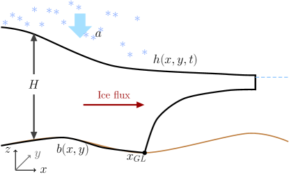
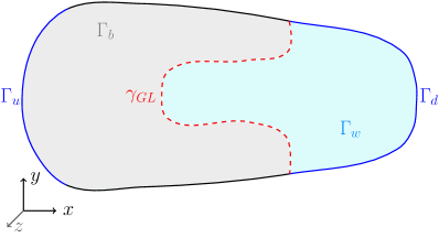
Figure 1: A schematic view of an ice sheet in the $x-z$ (left panel) and $x-y$ (right panel) plane.

Let $u_{1},u_{2},$ and $u_{3}$ be the velocity components of $\mathbf{u}=(u_{1},u_{2},u_{3})^{T}$ in the $x,y$ and $z$ directions and $\mathbf{x}=(x,y,z)^{T}$ in three dimensions. Vectors and matrices are written in bold characters. The horizontal plane is spanned by the $x$ and $y$ coordinates and $z$ is the coordinate in the vertical direction. Let the subscript $x,y,z$ or $t$ denote a derivative with respect to the variable. The height of the upper surface is $h(x,y,t)$, the $z$ coordinates of the bedrock and the floating interface are $b(x,y)$ and $z_{b}(x,y,t)$, and the ice thickness is $H=h-b$, as shown in Fig. 1.

The strain rate $\mathbf{D}$ and the viscosity $\eta$ are given by

$$\begin{array}[]{rll}\mathbf{D}(\mathbf{u})=\frac{1}{2}(\nabla\mathbf{u}+\nabla\mathbf{u}^{T}),\;\eta(\mathbf{u})=\frac{1}{2}{A}^{-\frac{1}{n}}({\rm tr}\mathbf{D}^{2}(\mathbf{u}))^{\nu},\;\nu=\frac{1-n}{2n},\end{array}$$ (1)

where ${\rm tr}\mathbf{D}^{2}$ is the trace of $\mathbf{D}^{2}$. The rate factor ${A}$ in (1) depends on the temperature and Glen’s flow law determines $n>0$, here taken to be $n=3$. The stress tensor is

$$\boldsymbol{\sigma}(\mathbf{u},p)=2\eta\mathbf{D}(\mathbf{u})-\mathbf{I}p,$$ (2)

where $p$ is the pressure and $\mathbf{I}$ is the identity matrix. The domain occupied by the ice is $\Omega$ with boundary $\Gamma$ whose outward pointing normal is $\mathbf{n}$. If $\mathbf{x}\in\Omega$ then $(x,y)\in\omega$ in the $x-y$ plane. The upper boundary is $\Gamma_{s}$ at the ice surface. The vertical, lateral boundary has an upstream part $\Gamma_{u}$ where $\mathbf{n}\cdot\mathbf{u}\leq 0$ and a downstream part $\Gamma_{d}$ where $\mathbf{n}\cdot\mathbf{u}>0$. The lower boundary at the bedrock is $\Gamma_{b}$ and the floating boundary is $\Gamma_{w}$. They are separated by the grounding line $\gamma_{GL}$ defined by $(x_{GL}(y),y)$ by assuming that the ice mainly flows along the $x$-axis. If $\mathbf{x}\in\Gamma_{u}$ or $\mathbf{x}\in\Gamma_{d}$ then $(x,y)\in\gamma_{u}$ or $(x,y)\in\gamma_{d}$ where $\gamma=\gamma_{u}\cup\gamma_{d}$ is the boundary of $\omega$. The definitions of these domains are

$$\begin{array}[]{rll}\Omega&=\{\mathbf{x}|(x,y)\in\omega,\,b(x,y)\leq z\leq h(x,y,t)\},\\ \Gamma_{s}&=\{\mathbf{x}|(x,y)\in\omega,\,z=h(x,y,t)\},\\ \Gamma_{b}&=\{\mathbf{x}|(x,y)\in\omega,\,z=b(x,y),\,x<x_{GL}(y)\},\\ \Gamma_{w}&=\{\mathbf{x}|(x,y)\in\omega,\,z=z_{b}(x,y,t),\,x>x_{GL}(y)\},\\ \Gamma_{u}&=\{\mathbf{x}|(x,y)\in\gamma_{u},\,b(x,y)\leq z\leq h(x,y,t)\},\\ \Gamma_{d}&=\{\mathbf{x}|(x,y)\in\gamma_{d},\,b(x,y)\leq z\leq h(x,y,t)\},\end{array}$$ (3)

and a schematic view in the $x-y$ plane is shown in the right panel of Fig. 1.

In two vertical dimensions as in the left panel of Fig. 1, $\mathbf{x}=(x,z)^{T},\;\omega=[0,L],\;\gamma_{u}=0,$ and $\gamma_{d}=L$ where $L$ is the horizontal length of the domain.

The basal stress on $\Gamma_{b}$ is related to the basal velocity using an empirical friction law. The friction coefficient has a general form $\beta(\mathbf{u},\mathbf{x},t)=C(\mathbf{x},t)f(\mathbf{u})$ where the coefficient $C(\mathbf{x},t)$ is independent of the velocity $\mathbf{u}$ and $f(\mathbf{u})$ represents some linear or nonlinear function of $\mathbf{u}$. For instance, $f(\mathbf{u})=\|\mathbf{u}\|^{m-1}$ with the norm $\|\mathbf{u}\|=(\mathbf{u}\cdot\mathbf{u})^{1/2}$ introduces a Weertman type friction law (Weertman 1957) on $\omega$ with a Weertman friction coefficient $C(\mathbf{x},t)>0$ and an exponent parameter $m>0$. Common choices of $m$ are $1/3$ and $1$.

The density of the ice is denoted by $\rho$, the accumulation/ablation rate on $\Gamma_{s}$ by $a$, and the gravitational acceleration by $\mathbf{g}$. A projection (Petra et al. 2012) on the tangential plane of $\Gamma_{b}$ is denoted by $\mathbf{T}=\mathbf{I}-\mathbf{n}\otimes\mathbf{n}$ where the Kronecker outer product between two vectors $\mathbf{a}$ and $\mathbf{c}$ or two matrices $\mathbf{A}$ and $\mathbf{C}$ is defined by

$$(\mathbf{a}\otimes\mathbf{c})_{ij}=a_{i}c_{j},\quad(\mathbf{A}\otimes\mathbf{C})_{ijkl}=A_{ij}C_{kl}.$$ (4)

With $\mathbf{h}=(h_{x},h_{y},-1)^{T}$ (in two dimensions $\mathbf{h}=(h_{x},-1)^{T}$), the forward FS equations for the height and velocity are

$$\begin{array}[]{rll}&h_{t}+\mathbf{h}\cdot\mathbf{u}=a,\;\;{\rm on}\;\Gamma_{s},\\ &h(\mathbf{x},0)=h_{0}(\mathbf{x}),\;\mathbf{x}\in\omega,\quad h(\mathbf{x},t)=h_{\gamma}(\mathbf{x},t),\;\mathbf{x}\in\gamma_{u},\\ &-\nabla\cdot\boldsymbol{\sigma}(\mathbf{u},p)=-\nabla\cdot(2\eta(\mathbf{u})\mathbf{D}(\mathbf{u}))+\nabla p=\rho\mathbf{g},\quad\nabla\cdot\mathbf{u}=0,\;{\rm in}\;\Omega(t),\\ &\boldsymbol{\sigma}\mathbf{n}=\mathbf{0},\;{\rm on}\;\Gamma_{s},\\ &\mathbf{T}\boldsymbol{\sigma}\mathbf{n}=-Cf(\mathbf{T}\mathbf{u})\mathbf{T}\mathbf{u},\quad\mathbf{n}\cdot\mathbf{u}=0,\;{\rm on}\;\Gamma_{b},\end{array}$$ (5)

where $h_{0}(\mathbf{x})$ is the initial height and $h_{\gamma}(\mathbf{x},t)$ is a given height on the inflow boundary. The boundary conditions of the velocity on $\Gamma_{u}$ and $\Gamma_{d}$ are of Dirichlet type such that

$$\mathbf{u}|_{\Gamma_{u}}=\mathbf{u}_{u},\quad\mathbf{u}|_{\Gamma_{d}}=\mathbf{u}_{d},$$ (6)

where $\mathbf{u}_{u}$ and $\mathbf{u}_{d}$ are some known velocities. In a special case where $\Gamma_{u}$ is at the ice divide, the horizontal velocity is set to $\mathbf{u}|_{\Gamma_{u}}=\mathbf{0}$, and the vertical component of $\boldsymbol{\sigma}\mathbf{n}$ also vanishes on $\Gamma_{u}$.

2.2 Shallow shelf approximation

On the ice shelf and the fast flowing region, the basal shear stress is negligibly small and the horizontal velocity is almost constant in the $z$ direction (Greve and Blatter 2009, MacAyeal 1989, Schoof 2007). The three dimensional FS problem (LABEL:eq:FSforw) on $\Omega$ can be simplified to a two dimensional, horizontal problem with $\mathbf{x}=(x,y)\in\omega$ by SSA, where only the horizontal velocity components $\mathbf{u}=(u_{1},u_{2})^{T}$ are considered. The viscosity for the SSA is

$$\eta(\mathbf{u})=\frac{1}{2}A^{-\frac{1}{n}}\left(u_{1x}^{2}+u_{2y}^{2}+\frac{1}{4}(u_{1y}+u_{2x})^{2}+u_{1x}u_{2y}\right)^{\nu}=\frac{1}{2}A^{-\frac{1}{n}}\left(\frac{1}{2}\mathbf{B}:\mathbf{D}\right)^{\nu},$$ (7)

where $\mathbf{B}(\mathbf{u})=\mathbf{D}(\mathbf{u})+\nabla\cdot\mathbf{u}\,\mathbf{I}$ with $\nabla\cdot\mathbf{u}={\rm tr}\,\mathbf{D}(\mathbf{u})$. The Frobenius inner product between two matrices $\mathbf{A}$ and $\mathbf{C}$ is defined by

$$\mathbf{A}:\mathbf{C}=\sum_{ij}A_{ij}C_{ij}.$$ (8)

The vertically integrated stress tensor $\boldsymbol{\varsigma}(\mathbf{u})$ is given by

$$\boldsymbol{\varsigma}(\mathbf{u})=2H\eta\mathbf{B}(\mathbf{u}),$$ (9)

Let $\mathbf{n}$ be the outward normal vector of the boundary $\gamma=\gamma_{u}\cup\gamma_{d}$ and $\mathbf{t}$ the tangential vector such that $\mathbf{n}\cdot\mathbf{t}=0$. The friction law is defined as in the FS case where the basal velocity is replaced by the horizontal velocity since the vertical variation is neglected in SSA. An example is Weertman’s law defined by $\beta(\mathbf{u},\mathbf{x},t)=C(\mathbf{x},t)f(\mathbf{u})=C(\mathbf{x},t)\|\mathbf{u}\|^{m-1}$ with a friction coefficient $C(\mathbf{x},t)\geq 0$. In Fig. 1, $\omega=\Gamma_{b}\cup\Gamma_{w}$ and $\gamma_{u}=\Gamma_{u},\,\gamma_{d}=\Gamma_{d}$.

The ice dynamics system is

$$\begin{array}[]{rll}&h_{t}+\nabla\cdot(\mathbf{u}H)=a,\;\;0\leq t\leq T,\;\mathbf{x}\in\omega,\\ &h(\mathbf{x},0)=h_{0}(\mathbf{x}),\;\mathbf{x}\in\omega,\quad h(\mathbf{x},t)=h_{\gamma}(\mathbf{x},t),\,\mathbf{x}\in\gamma_{u},\\ &\nabla\cdot\boldsymbol{\varsigma}-Cf(\mathbf{u})\mathbf{u}=\rho gH\nabla h,\;\mathbf{x}\in\omega,\\ &\mathbf{n}\cdot\mathbf{u}(\mathbf{x},t)=u_{u}(\mathbf{x},t),\mathbf{x}\in\gamma_{u},\quad\mathbf{n}\cdot\mathbf{u}(\mathbf{x},t)=u_{d}(\mathbf{x},t),\mathbf{x}\in\gamma_{d},\\ &\mathbf{t}\cdot\boldsymbol{\varsigma}\mathbf{n}=-C_{\gamma}f_{\gamma}(\mathbf{t}\cdot\mathbf{u})\mathbf{t}\cdot\mathbf{u},\;\mathbf{x}\in\gamma_{g},\quad\mathbf{t}\cdot\boldsymbol{\varsigma}\mathbf{n}=0,\;\mathbf{x}\in\gamma_{w}.\end{array}$$ (10)

The inflow and outflow normal velocities $u_{u}\leq 0$ and $u_{d}>0$ are specified on $\gamma_{u}$ and $\gamma_{d}$. The lateral side of the ice $\gamma$ is split into $\gamma_{g}$ and $\gamma_{w}$ with $\gamma=\gamma_{g}\cup\gamma_{w}$. There is friction in the tangential direction on $\gamma_{g}$ which depends on the tangential velocity $\mathbf{t}\cdot\mathbf{u}$ with the friction coefficient $C_{\gamma}$ and friction function $f_{\gamma}$. There is no friction on $\gamma_{w}$. The structure of the SSA system (LABEL:eq:SSAforw3D) is similar to the FS equations in (LABEL:eq:FSforw). However, the velocity $\mathbf{u}$ is not divergence free in SSA and $\mathbf{B}\neq\mathbf{D}$ due to the cryostatic approximation of $p$.

In the case where an ice shelf or a grounding line exists, the floating ice is assumed to be at hydrostatic equilibrium in the seawater. A calving front boundary condition (Schoof 2007, van der Veen 1996) is applied at $\gamma_{d}$ by the depth integrated stress balance

$$\boldsymbol{\varsigma}(\mathbf{u})\cdot\mathbf{n}=\frac{1}{2}\rho gH^{2}\left(1-\frac{\rho}{\rho_{w}}\right)\mathbf{n},\;\mathbf{x}\in\gamma_{d},$$ (11)

where $\rho_{w}$ is the density of seawater. With this boundary condition, a calving rate $u_{c}$ can be determined at the ice front.

3 Adjoint equations

We wish to determine the sensitivity of a functional

$$\mathcal{F}=\int_{0}^{T}\int_{\Gamma_{s}}F(\mathbf{u},h)\,\text{d}\mathbf{x}\,\text{d}t$$ (12)

at $\Gamma_{s}$ in the time interval $[0,T]$ to perturbations in the friction coefficient $C(\mathbf{x},t)$ at the base of the ice and the topography $b(\mathbf{x})$ when $\mathbf{u}$ and $h$ satisfy the FS equations (LABEL:eq:FSforw) or the SSA equations (LABEL:eq:SSAforw3D). We introduce a Lagrangian $\mathcal{L}(\mathbf{u},p,h;\mathbf{v},q,\psi;b,C)$ for a given observation $\mathcal{F}$ with the forward solution $(\mathbf{u},p,h)$ to (LABEL:eq:FSforw) or $(\mathbf{u},h)$ to (LABEL:eq:SSAforw3D) and the corresponding adjoint solutions $(\mathbf{v},q,\psi)$ or $(\mathbf{v},\psi)$. The adjoint solutions solve the adjoint equations to the FS and SSA equations. These equations will be derived using the Lagrangian in this section and Appendix A.

The effect of the perturbations $\delta C$ and $\delta b$ in $C$ and $b$ on $\mathcal{F}$ is given by the perturbation $\delta\mathcal{L}$ in the Lagrangian

$$\begin{array}[]{lll}\delta\mathcal{F}&=\delta\mathcal{L}\\ &=\mathcal{L}(\mathbf{u}+\delta\mathbf{u},p+\delta p,h+\delta h;\mathbf{v}+\delta\mathbf{v},q+\delta q,\psi+\delta\psi;b+\delta b,C+\delta C)\\ &\quad-\mathcal{L}(\mathbf{u},p,h;\mathbf{v},q,\psi;b,C).\end{array}$$

Examples of $F(\mathbf{u},h)$ in (12) are $\|\mathbf{u}-\mathbf{u}_{\rm obs}\|^{2}$, $|h-h_{\rm obs}|^{2}$ in an inverse problem to find $b$ and $C$ to match the observed data $\mathbf{u}_{\rm obs}$ and $h_{\rm obs}$ at the surface $\Gamma_{s}$ as in (Gillet-Chaulet et al. 2016, Isaac et al. 2015, Morlighem et al. 2013, Petra et al. 2012), or $F(\mathbf{u},h)=\frac{1}{T}u_{1}(\mathbf{x},t)\delta(\mathbf{x}-\mathbf{x}_{\ast})$ with the Dirac delta at $\mathbf{x}_{\ast}$ to measure the time averaged deviation of the horizontal velocity $u_{1}$ at $\mathbf{x}_{\ast}$ on the ice surface $\Gamma_{s}$ with

$$\mathcal{F}=\int_{0}^{T}\int_{\Gamma_{s}}F(\mathbf{u},h)\,\text{d}\mathbf{x}\,\text{d}t=\frac{1}{T}\int_{0}^{T}u_{1}(\mathbf{x}_{\ast},t)\,\text{d}t,$$

where $T$ is the duration of the observation at $\Gamma_{s}$.

3.1 Full Stokes equation

The definition of the Lagrangian $\mathcal{L}$ for the FS equations is found in (LABEL:eq:FSLag) in Appendix A where $(\mathbf{v},q,\psi)$ are the Lagrange multipliers corresponding to the forward equations for $(\mathbf{u},p,h)$. In order to determine $(\mathbf{v},q,\psi)$, the so-called adjoint problem is solved

$$\begin{array}[]{rll}&\psi_{t}+\nabla\cdot(\mathbf{u}\psi)-\mathbf{h}\cdot\mathbf{u}_{z}\psi=F_{h}+F_{\mathbf{u}}\cdot\mathbf{u}_{z},\;\;{\rm on}\;\Gamma_{s},\\ &\psi(\mathbf{x},T)=0,\;\psi(\mathbf{x},t)=0,\;{\rm on}\;\Gamma_{d},\\ &-\nabla\cdot\tilde{\boldsymbol{\sigma}}(\mathbf{v},q)=-\nabla\cdot(2\tilde{\boldsymbol{\eta}}(\mathbf{u})\star\mathbf{D}(\mathbf{v}))+\nabla q=\mathbf{0},\quad\nabla\cdot\mathbf{v}=0,\;{\rm in}\;\Omega(t),\\ &\tilde{\boldsymbol{\sigma}}(\mathbf{v},q)\mathbf{n}=-(F_{\mathbf{u}}+\psi\mathbf{h}),\;{\rm on}\;\Gamma_{s},\\ &\mathbf{T}\tilde{\boldsymbol{\sigma}}(\mathbf{v},q)\mathbf{n}=-Cf(\mathbf{T}\mathbf{u})\left(\mathbf{I}+\mathbf{F}_{b}(\mathbf{T}\mathbf{u})\right)\mathbf{T}\mathbf{v},\;{\rm on}\;\Gamma_{b},\\ &\mathbf{n}\cdot\mathbf{v}=0,\;{\rm on}\;\Gamma_{b},\end{array}$$ (13)

where the derivatives of $F$ with respect to $\mathbf{u}$ and $h$ are

$$F_{\mathbf{u}}=\left(\frac{\partial F}{\partial u_{1}},\frac{\partial F}{\partial u_{2}},\frac{\partial F}{\partial u_{3}}\right)^{T},\quad F_{h}=\frac{\partial F}{\partial h}.$$

The adjoint viscosity and adjoint stress (Petra et al. 2012) are

$$\begin{array}[]{rll}\tilde{\boldsymbol{\eta}}(\mathbf{u})&=\eta(\mathbf{u})\left(\mathcal{I}+\frac{1-n}{n\mathbf{D}(\mathbf{u}):\mathbf{D}(\mathbf{u})}\mathbf{D}(\mathbf{u})\otimes\mathbf{D}(\mathbf{u})\right),\\ \tilde{\boldsymbol{\sigma}}(\mathbf{v},q)&=2\tilde{\boldsymbol{\eta}}(\mathbf{u})\star\mathbf{D}(\mathbf{v})-q\mathbf{I}.\\ \end{array}$$ (14)

The tensor $\mathcal{I}$ has four indices $ijkl$ and $\mathcal{I}_{ijkl}=1$ only when $i=j=k=l$, otherwise $\mathcal{I}_{ijkl}=0$. In general, $\mathbf{F}_{b}(\mathbf{T}\mathbf{u})$ in (LABEL:eq:FSadj) is a linearization of the friction law relation $f(\mathbf{T}\mathbf{u})$ in (LABEL:eq:FSforw) with respect to the variable $\mathbf{T}\mathbf{u}$. For instance, with a Weertman type friction law, $f(\mathbf{T}\mathbf{u})=\|\mathbf{T}\mathbf{u}\|^{m-1}$, it is

$$\mathbf{F}_{b}(\mathbf{T}\mathbf{u})=\frac{m-1}{\mathbf{T}\mathbf{u}\cdot\mathbf{T}\mathbf{u}}(\mathbf{T}\mathbf{u})\otimes(\mathbf{T}\mathbf{u}).$$ (15)

The $\star$ operation in (14) between a four index tensor $\mathcal{A}$ and a two index tensor or matrix $\mathbf{C}$ is defined by

$$(\mathcal{A}\star\mathbf{C})_{ij}=\sum_{kl}\mathcal{A}_{ijkl}C_{kl}.$$ (16)

The perturbation of the Lagrangian function with respect to a perturbation $\delta C$ in the slip coefficient $C(\mathbf{x},t)$ is

$$\delta\mathcal{F}=\delta\mathcal{L}=\int_{0}^{T}\int_{\Gamma_{b}}f(\mathbf{T}\mathbf{u})\mathbf{T}\mathbf{u}\cdot\mathbf{T}\mathbf{v}\,\,\delta C\,\,\text{d}\mathbf{x}\,\text{d}t$$ (17)

involving the tangential components of the forward and adjoint velocities $\mathbf{T}\mathbf{u}$ and $\mathbf{T}\mathbf{v}$ at the ice base $\Gamma_{b}$.

The detailed derivation of the adjoint equations (LABEL:eq:FSadj) and the perturbation of the Lagrangian function (17) are given in Appendix A.3 from the weak form of the FS equations (LABEL:eq:FSforw) on $\Omega$, integration by parts, and by applying the boundary conditions as in (Martin and Monnier 2014, Petra et al. 2012). The adjoint equations consist of the equations for the adjoint height $\psi$, the adjoint velocity $\mathbf{v}$, and the adjoint pressure $q$. Compared to the steady state adjoint equation for the FS equation in (Petra et al. 2012), an advection equation is added in (LABEL:eq:FSadj) for the Lagrange multiplier $\psi(\mathbf{x},t)$ on $\Gamma_{s}$ with a right hand side depending on the observation function $F$ and one term depending on $\psi$ in the boundary condition on $\Gamma_{s}$. The adjoint height equation of $\psi$ can be solved independently of the adjoint stress equation since it is independent of $\mathbf{v}$. If $h$ is observed then the adjoint height equation must be solved together with the adjoint stress equation. Otherwise, the term $\psi\mathbf{h}$ vanishes in the right hand side of the adjoint stress equation and the solution is $\mathbf{v}=\mathbf{0}$ with $\delta\mathcal{F}=0$ in (17).

3.1.1 Time-dependent perturbations

Suppose that $u_{1\ast}=u_{1}(\mathbf{x}_{\ast},t_{\ast})$ is observed at $(\mathbf{x}_{\ast},t_{\ast})$ at the ice surface and that $t_{\ast}<T$, then

$$u_{1}(\mathbf{x}_{\ast},t_{\ast})=\mathcal{F}=\int_{0}^{T}\int_{\Gamma_{s}}F(\mathbf{u})\,\text{d}\mathbf{x}\,\text{d}t,$$

with

$$F(\mathbf{u})=u_{1}\delta(\mathbf{x}-\mathbf{x}_{\ast})\delta(t-t_{\ast}),\;F_{u_{1}}=\delta(\mathbf{x}-\mathbf{x}_{\ast})\delta(t-t_{\ast}),\;F_{u_{2}}=F_{u_{3}}=0,\;F_{h}=0.$$

The procedure to determine the sensitivity is as follows. First, the forward equation (LABEL:eq:FSforw) is solved for $\mathbf{u}(\mathbf{x},t)$ from $t=0$ to $t=T$. Then, the adjoint equation (LABEL:eq:FSadj) is solved backward in time for $t\leq T$ with $\psi(\mathbf{x},T)=0$ as the final condition. Obviously, the solution for $t_{\ast}<t\leq T$ is $\psi(\mathbf{x},t)=0$ and $\mathbf{v}(\mathbf{x},t)=\mathbf{0}$. Denote the unit vector with 1 in the $i$:th component by $\mathbf{e}^{i}$. At $t=t_{\ast}$ we have

$$\tilde{\boldsymbol{\sigma}}(\mathbf{v},q)\mathbf{n}=-\mathbf{e}^{1}\delta(\mathbf{x}-\mathbf{x}_{\ast})\delta(t-t_{\ast})-\psi\mathbf{h},$$

in the boundary condition in (LABEL:eq:FSadj). For $t<t_{\ast}$, $\tilde{\boldsymbol{\sigma}}(\mathbf{v},q)\mathbf{n}=-\psi\mathbf{h}$. Since $\psi$ is small for $t<t_{\ast}$ (see Sect. 3.1.3), the dominant part of the solution is $\mathbf{v}(\mathbf{x},t)=\mathbf{v}_{0}(\mathbf{x})\delta(t-t_{\ast})$ for some $\mathbf{v}_{0}$. To simplify the notation in the remainder of this paper, a variable with the subscript $\ast$ is evaluated at $(\mathbf{x}_{\ast},t_{\ast})$ or if it is time independent at $x_{\ast}$.

When the slip coefficient at the ice base is changed by $\delta C$, then the change in $u_{1\ast}$ is by (17)

$$\begin{array}[]{rll}\delta u_{1\ast}&=\delta\mathcal{L}=\displaystyle{\int_{0}^{T}\int_{\Gamma_{b}}f(\mathbf{T}\mathbf{u})\mathbf{T}\mathbf{u}\cdot\mathbf{T}\mathbf{v}\,\delta C\,\text{d}\mathbf{x}\,\text{d}t}\\ &\displaystyle{\approx\int_{\Gamma_{b}}f(\mathbf{T}\mathbf{u})\mathbf{T}\mathbf{u}\cdot\mathbf{T}\mathbf{v}_{0}\,\delta C(\mathbf{x},t_{\ast})\,\text{d}\mathbf{x}.}\end{array}$$ (18)

In this case, the perturbation $\delta u_{1\ast}$ mainly depends on $\delta C$ at time $t_{\ast}$ and the contribution from previous $\delta C(\mathbf{x},t),\,t<t_{\ast},$ is small.

Let the height $h_{\ast}$ be measured at $\Gamma_{s}$. Then

$$F(h)=h(x,t)\delta(\mathbf{x}-\mathbf{x}_{\ast})\delta(t-t_{\ast}),\;F_{h}=\delta(\mathbf{x}-\mathbf{x}_{\ast})\delta(t-t_{\ast}),\;F_{\mathbf{u}}=\mathbf{0}.$$

The solution of the adjoint equation (LABEL:eq:FSadj) with $\tilde{\boldsymbol{\sigma}}(\mathbf{v},q)\mathbf{n}=-\psi\mathbf{h}$ at $\Gamma_{s}$ for $\mathbf{v}(\mathbf{x},t)$ is non-zero since $\psi(\mathbf{x},t)\neq 0$ for $t<t_{\ast}$. In a seasonal variation, there is a time dependent perturbation $\delta C(\mathbf{x},t)=\delta C_{0}(\mathbf{x})\cos(2\pi t/\tau)$ added to a stationary time average $C(\mathbf{x})$. The time constant $\tau$ could be for example 1 a (year). Assume that $f(\mathbf{T}\mathbf{u})\mathbf{T}\mathbf{u}\cdot\mathbf{T}\mathbf{v}$ is approximately constant in time (e.g. if $\mathbf{u}$ varies slowly, then $\psi\approx{\rm const}$ and $\mathbf{v}\approx{\rm const}$ for $t<t_{\ast}$. Then the observation at the ice surface varies as

$$\begin{array}[]{rll}\delta h_{\ast}&\displaystyle{=\delta\mathcal{L}=\int_{0}^{T}\int_{\Gamma_{b}}f(\mathbf{T}\mathbf{u})\mathbf{T}\mathbf{u}\cdot\mathbf{T}\mathbf{v}\,\delta C(\mathbf{x},t)\,\text{d}\mathbf{x}\,\text{d}t}\\ &\displaystyle{\approx\int_{0}^{t_{\ast}}\cos(2\pi t/\tau)\,\text{d}t\int_{\Gamma_{b}}f(\mathbf{T}\mathbf{u})\mathbf{T}\mathbf{u}\cdot\mathbf{T}\mathbf{v}\,\delta C_{0}\,\text{d}\mathbf{x}}\\ &\displaystyle{=\frac{\tau}{2\pi}\sin(2\pi t_{\ast}/\tau)\int_{\Gamma_{b}}f(\mathbf{T}\mathbf{u})\mathbf{T}\mathbf{u}\cdot\mathbf{T}\mathbf{v}\,\delta C_{0}\,\text{d}\mathbf{x}}.\end{array}$$ (19)

When the friction perturbation $\delta C$ is large at $t_{\ast}=0,\tau/2,\tau\ldots,$ the effect on $h_{\ast}$ vanishes. If the middle of the winter is at $n\tau,\;n=0,1,2,\ldots$, then the middle of the summer is at $(n+1/2)\tau$. The friction is at its maximum in the winter and at its minimum in the summer when the meltwater introduces lubrication. There is no change of $h_{\ast}$ in the middle of the summer, $\delta h_{\ast}=0$, but $C+\delta C$ has its lowest value then. If $h_{\ast}$ is measured in the summer and compared to a mean value $h(\mathbf{x})$, then $\delta h(\mathbf{x},t_{\ast})=0$ and the wrong conclusion would be drawn that there is no change in $C$ if the phase shift between $\delta C$ and $\delta h$ in (19) is not accounted for.

A two dimensional numerical example is shown in Fig. 2 with $\tau=1$ a and $\delta C(x,t)=0.01C\cos(2\pi t)$ in an interval $x\in[0.9,1.0]\times 10^{6}$ m where the ice sheet flows from $x=0$ to $L=1.6\times 10^{6}$ m. The grounding line is at $x_{GL}=1.035\times 10^{6}$ m. The details of the setup are found in the MISMIP (Pattyn et al. 2012) test case used in (Cheng and Lötstedt 2019). The ice sheet is simulated by FS with Elmer/Ice (Gagliardini et al. 2013) for 10 years. The perturbations in $\delta u_{1}$ and $\delta h$ oscillate regularly with a period of 1 year after an initial transient and are small outside the interval $[0.9,1.0]\times 10^{6}$. An increase in the friction, $\delta C>0$, leads to a decrease in the velocity and $\delta C<0$ increases the velocity. There is a phase shift $\Delta\phi$ in time by $\pi/2$ between $\delta u$ and $\delta h$ as predicted by (18) and (19). The weight in (19) for $\delta C_{0}$ in the integral over $\mathbf{x}$ changes sign when the observation point is passing from $x_{\ast}=0.9\times 10^{6}$ to $1.0\times 10^{6}$ explaining why the shift changes sign in the two lower panels.

The phase shift $\Delta\phi$ between the surface observations and the basal perturbations is investigated in (Gudmundsson 2003) with a linearized equation and Fourier analysis. It is found that $\Delta\phi=-\pi/2$ between $\delta C$ and $\delta h$ for short perturbation wave lengths in the steady state as in Fig. 2.

Figure 2: Observations at $x_{\ast}=0.85,0.9,0.95,1.0,1.02\times 10^{6}$ m with FS in time $t\in[0,10]$ of $\delta u_{1}$(blue) and $\delta h$(red) with perturbation $\delta C(t)=0.01C\cos(2\pi t)$ for $x\in[0.9,1.0]\times 10^{6}$ m. Notice the different scales on the $y$-axes.

3.1.2 The sensitivity problem and the inverse problem

There is a relation between the sensitivity problem and the inverse problem to infer parameters from data. Assume that $({\mathbf{v}}^{i},{q}^{i},{\psi}^{i}),i=1,\ldots,d,$ solves (LABEL:eq:FSadj) with $F_{\mathbf{u}}=\mathbf{e}^{i}\delta(\mathbf{x}-\bar{\mathbf{x}})$ or $F_{h}=\delta(\mathbf{x}-\bar{\mathbf{x}})$. With $F_{\mathbf{u}}\neq 0,F_{h}=0$ we have $d=2\,(\text{or }3)$ in two (three)-dimensions and with $F_{\mathbf{u}}=0,F_{h}\neq 0$ we have $d=1$. Consider a target functional $\mathcal{F}$ for the steady state solution with weights $w_{i}(\bar{\mathbf{x}})$ multiplying $\delta u^{i}$ in the first variation of $\mathcal{F}$. Using (17), $\delta\mathcal{F}$ is

$$\begin{array}[]{rll}\delta\mathcal{F}&=\displaystyle{\int_{\omega}\sum_{i=1}^{d}w_{i}(\bar{\mathbf{x}})\delta u^{i}\,\text{d}\bar{\mathbf{x}}=\int_{\omega}\sum_{i=1}^{d}w_{i}(\bar{\mathbf{x}})\int_{\Gamma_{b}}f(\mathbf{T}\mathbf{u})\mathbf{T}\mathbf{u}\cdot\mathbf{T}{\mathbf{v}}^{i}\,\delta C\,\text{d}\mathbf{x}\,\text{d}\bar{\mathbf{x}}}\\ &=\displaystyle{\int_{\Gamma_{b}}f(\mathbf{T}\mathbf{u})\mathbf{T}\mathbf{u}\cdot\mathbf{T}\left(\int_{\omega}\sum_{i=1}^{d}w_{i}(\bar{\mathbf{x}}){\mathbf{v}}^{i}\,\text{d}\bar{\mathbf{x}}\right)\,\delta C\,\text{d}\mathbf{x}.}\end{array}$$ (20)

It follows from (LABEL:eq:FSadj) that $(w_{i}(\bar{\mathbf{x}}){\mathbf{v}}^{i}(\mathbf{x}),w_{i}(\bar{\mathbf{x}}){q}^{i}(\mathbf{x}),w_{i}(\bar{\mathbf{x}}){\psi}^{i}(\mathbf{x}))$ is a solution with $F_{\mathbf{u}}=w_{i}(\bar{\mathbf{x}})\mathbf{e}^{i}\delta(\mathbf{x}-\bar{\mathbf{x}})$ or $F_{h}=w(\bar{\mathbf{x}})\delta(\mathbf{x}-\bar{\mathbf{x}})$. Therefore, also

$$\left(\int_{\omega}w_{i}(\bar{\mathbf{x}}){\mathbf{v}}^{i}\,\text{d}\bar{\mathbf{x}},\int_{\omega}w_{i}(\bar{\mathbf{x}}){q}^{i}\,\text{d}\bar{\mathbf{x}},\int_{\omega}w_{i}(\bar{\mathbf{x}}){\psi}^{i}\,\text{d}\bar{\mathbf{x}}\right)$$

is a solution with $F_{\mathbf{u}}=\int_{\omega}w_{i}(\bar{\mathbf{x}})\mathbf{e}^{i}\delta(\mathbf{x}-\bar{\mathbf{x}})\,\text{d}\bar{\mathbf{x}}=w_{i}(\mathbf{x})\mathbf{e}^{i}$ or $F_{h}=\int_{\omega}w(\bar{\mathbf{x}})\delta(\mathbf{x}-\bar{\mathbf{x}})\,\text{d}\bar{\mathbf{x}}=w(\mathbf{x})$.

In the inverse problem, $\mathcal{F}=\frac{1}{2}\int_{\omega}\|\mathbf{u}(\mathbf{x})-\mathbf{u}_{\rm obs}(\mathbf{x})\|^{2}\,\text{d}\mathbf{x}$ (Petra et al. 2012) and the first variation is $\delta\mathcal{F}=\int_{\omega}(\mathbf{u}(\mathbf{x})-\mathbf{u}_{\rm obs}(\mathbf{x}))\cdot\delta\mathbf{u}(\mathbf{x})\,\text{d}\mathbf{x}$. Let $w_{i}(\mathbf{x})=u_{i}(\mathbf{x})-u_{{\rm obs},i}(\mathbf{x})$ in (20). Then we find that

$$\delta\mathcal{F}=\int_{\Gamma_{b}}f(\mathbf{T}\mathbf{u})\mathbf{T}\mathbf{u}\cdot\mathbf{T}\tilde{\mathbf{v}}(\mathbf{x})\,\delta C\,\text{d}\mathbf{x},$$ (21)

where

$$\tilde{\mathbf{v}}(\mathbf{x})=\int_{\omega}\sum_{i=1}^{d}w_{i}(\bar{\mathbf{x}}){\mathbf{v}}^{i}(\mathbf{x})\,\text{d}\bar{\mathbf{x}}$$

is a solution to (LABEL:eq:FSadj) with $F_{\mathbf{u}}=(w_{1},w_{2},w_{3})^{T}=\mathbf{u}-\mathbf{u}_{\rm obs}$ or $F_{h}=w=h-h_{\rm obs}$.

If we are interested in solving the inverse problem and determine $\delta\mathcal{F}$ in (20) to iteratively compute the optimal solution with a gradient method, then we solve (LABEL:eq:FSadj) directly with $F_{\mathbf{u}}=\mathbf{u}-\mathbf{u}_{\rm obs}$ or $F_{h}=h-h_{\rm obs}$ to obtain $\tilde{\mathbf{v}}$ without computing ${\mathbf{v}}^{i}$.

3.1.3 Steady state solution to the adjoint height equation in two dimensions

In a two dimensional vertical ice, with $\mathbf{u}(x,z)=(u_{1},u_{3})^{T}$, the stationary equation for $\psi$ in (LABEL:eq:FSadj) is

$$(u_{1}\psi)_{x}=F_{h}+(\mathbf{h}\psi+F_{\mathbf{u}})\cdot\mathbf{u}_{z},\;z=h,\;0\leq x\leq L.$$ (22)

When $x>x_{\ast}$, where $F_{h}=0$ and $F_{\mathbf{u}}=0$, then $\psi(x)=0$ since the right boundary condition is $\psi(L)=0$.

If $u_{1}$ is observed at $\Gamma_{s}$ then $F(\mathbf{u},h)=u_{1}(x)\chi(x)$ and $F_{\mathbf{u}}=(\chi(x),0)^{T}$ and $F_{h}=0$. The weight $\chi$ on $u_{1}$ may be a Dirac delta, a Gaussian, or a constant in a limited interval. On the other hand, if $F(\mathbf{u},h)=h(x)\chi(x)$ then $F_{h}=\chi(x)$ and $F_{\mathbf{u}}=\mathbf{0}$.

Let $g(x)=u_{1z}(x)$ when $F_{\mathbf{u}}\neq\mathbf{0}$ and let $g(x)=1$ when $F_{h}\neq 0$. Then by (22)

$$(u_{1}\psi)_{x}-\mathbf{h}\cdot\mathbf{u}_{z}\psi=g(x)\chi(x).$$ (23)

The solution to (23) is

$$\begin{array}[]{rll}\psi(x)&=\displaystyle{-\frac{1}{u_{1}(x)}\int_{x}^{x_{\ast}}\exp\left(-\int_{x}^{\xi}\frac{\mathbf{h}\cdot\mathbf{u}_{z}(y)}{u_{1}(y)}\,\text{d}y\right)g(\xi)\chi(\xi)\,\text{d}\xi,\;0\leq x<x_{\ast},}\\ \psi(x)&=0,\;x_{\ast}<x\leq L.\end{array}$$ (24)

In particular, if $\chi(x)=\delta(x-x_{\ast})$ then $\mathcal{F}=u(x_{\ast})$ or $\mathcal{F}=h(x_{\ast})$ and the multiplier is

$$\psi(x)=-\frac{g(x_{\ast})}{u_{1}(x)}\exp\left(-\int_{x}^{x_{\ast}}\frac{\mathbf{h}\cdot\mathbf{u}_{z}(y)}{u_{1}(y)}\,\text{d}y\right),\;0\leq x<x_{\ast},$$ (25)

which has a jump $-g(x_{\ast})/u_{1}(x_{\ast})$ at $x_{\ast}$.

With a small $\mathbf{h}\cdot\mathbf{u}_{z}(y)\approx 0$ above, an approximate solution is $\psi(x)\approx-g(x_{\ast})/u_{1}(x)$. Moreover, if $\mathbf{u}$ is observed with $F_{\mathbf{u}}\neq 0$ and $g(\mathbf{x})\approx 0$, then $\psi(\mathbf{x})\approx 0$ and $\psi\mathbf{h}\approx 0$ in (LABEL:eq:FSadj). Consequently when $u_{1}$ is observed, the effect on $\mathbf{v}$ of the solution of the adjoint advection equation is negligible. It is sufficient to solve only the adjoint stress equation for $\mathbf{v}$ as in (Gillet-Chaulet et al. 2016, Isaac et al. 2015, Petra et al. 2012), which may often be the case in FS.

3.2 Shallow shelf approximation

The adjoint equations for SSA are given and analyzed in this section. A Lagrangian $\mathcal{L}$ of the SSA equations is defined with the same technique as in (Petra et al. 2012) for the FS equations. By evaluating $\mathcal{L}$ at the forward solution $(\mathbf{u},h)$ and the adjoint solution $(\mathbf{v},\psi)$, the effect of perturbed data at the ice base can be observed at the ice surface as a perturbation $\delta\mathcal{L}$. The details of the derivations are found in Appendix A.2. In a two dimensional vertical ice at the steady state, the equations are simpler and analytical solutions for the forward and adjoint equations are derived later in this section.

After insertion of the forward solution, partial integration in $\mathcal{L}$, and applying the boundary conditions, the adjoint SSA equations are obtained as

$$\begin{array}[]{rll}&\psi_{t}+\mathbf{u}\cdot\nabla\psi+2\eta\mathbf{B}(\mathbf{u}):\mathbf{D}(\mathbf{v})-\rho gH\nabla\cdot\mathbf{v}+\rho g\mathbf{v}\cdot\nabla b=F_{h},\;\;{\rm in}\;\omega,\\ &\psi(\mathbf{x},T)=0,\;\;{\rm in}\;\omega,\quad\psi(\mathbf{x},t)=0,\;\;{\rm on}\;\gamma_{w},\\ &\nabla\cdot\tilde{\boldsymbol{\varsigma}}(\mathbf{v})-Cf(\mathbf{u})(\mathbf{I}+\mathbf{F}_{\omega}(\mathbf{u}))\mathbf{v}-H\nabla\psi=-F_{\mathbf{u}},\quad{\rm in}\;\omega,\\ &\mathbf{t}\cdot\tilde{\boldsymbol{\varsigma}}(\mathbf{v})\mathbf{n}=-C_{\gamma}f_{\gamma}(\mathbf{t}\cdot\mathbf{u})(1+F_{\gamma}(\mathbf{t}\cdot\mathbf{u}))\mathbf{t}\cdot\mathbf{v},\;{\rm on}\;\gamma_{g},\quad\mathbf{t}\cdot\tilde{\boldsymbol{\varsigma}}(\mathbf{v})\mathbf{n}=0,\;{\rm on}\;\gamma_{w},\\ &\mathbf{n}\cdot\mathbf{v}=0,\;{\rm on}\;\gamma,\end{array}$$ (26)

where the adjoint viscosity $\tilde{\boldsymbol{\eta}}$ and adjoint stress $\tilde{\boldsymbol{\varsigma}}$ are defined by

$$\begin{array}[]{rll}\tilde{\boldsymbol{\eta}}(\mathbf{u})&=\eta(\mathbf{u})\left(\mathcal{I}+\frac{1-n}{n\mathbf{B}(\mathbf{u}):\mathbf{D}(\mathbf{u})}\mathbf{B}(\mathbf{u})\otimes\mathbf{D}(\mathbf{u})\right),\\ \tilde{\boldsymbol{\varsigma}}(\mathbf{v})&=2H\tilde{\boldsymbol{\eta}}(\mathbf{u})\star\mathbf{B}(\mathbf{v}),\end{array}$$ (27)

cf. $\tilde{\boldsymbol{\eta}}$ and $\tilde{\boldsymbol{\sigma}}$ of FS in (14). The adjoint equation derived in (MacAyeal 1993) is the stress equation in (LABEL:eq:SSAadj3D) with a constant $H$, $\mathbf{F}_{\omega}=0$ and $\tilde{\boldsymbol{\eta}}(\mathbf{u})=\eta(\mathbf{u})$.

The adjoint SSA equations have the same structure as the adjoint FS equations (LABEL:eq:FSadj). There is one stress equation for the adjoint velocity $\mathbf{v}$ and one equation for the multiplier $\psi$ corresponding to the height equation in (LABEL:eq:SSAforw3D). However, the advection equation for $\psi$ in (LABEL:eq:SSAadj3D) depends on the adjoint velocity $\mathbf{v}$ which leads to a fully coupled system for $\mathbf{v}$ and $\psi$.

The equations are solved backward in time with a final condition on $\psi$ at $t=T$. As in (LABEL:eq:SSAforw3D), there is no time derivative in the stress equation. With a Weertman friction law, $f(\mathbf{u})=\|\mathbf{u}\|^{m-1}$ and $f_{\gamma}(\mathbf{t}\cdot\mathbf{u})=|\mathbf{t}\cdot\mathbf{u}|^{m-1}$, it is shown in Appendix A.1 that

$$\mathbf{F}_{\omega}(\mathbf{u})=\frac{m-1}{\mathbf{u}\cdot\mathbf{u}}\mathbf{u}\otimes\mathbf{u},\quad F_{\gamma}=m-1.$$

If the friction coefficient $C$ at the ice base is changed by $\delta C$, the bottom topography is changed by $\delta b$, and the lateral friction coefficient $C_{\gamma}$ is changed by $\delta C_{\gamma}$, then it follows from Appendix A.2 that the Lagrangian is changed by

$$\begin{array}[]{rll}\delta\mathcal{L}=&\displaystyle{\int_{0}^{T}\int_{\omega}(2\eta\mathbf{B}(\mathbf{u}):\mathbf{D}(\mathbf{v})+\rho g\mathbf{v}\cdot\nabla h+\nabla\psi\cdot\mathbf{u})\,\delta b-f(\mathbf{u})\mathbf{u}\cdot\mathbf{v}\,\delta C\,\,\text{d}\mathbf{x}\,\text{d}t}\\ &\displaystyle{-\int_{0}^{T}\int_{\gamma_{g}}f_{\gamma}(\mathbf{t}\cdot\mathbf{u})\mathbf{t}\cdot\mathbf{u}\,\mathbf{t}\cdot\mathbf{v}\,\delta C_{\gamma}\,\text{d}s\,\text{d}t.}\end{array}$$ (28)

The weight in front of $\delta C$ in (28) is actually the same as in (17).

Suppose that $h$ is observed with $F_{\mathbf{u}}=0$ in (LABEL:eq:SSAadj3D). Then the adjoint height equation must be solved for $\psi\neq 0$ to have a $\mathbf{v}\neq\mathbf{0}$ in the adjoint stress equation and a perturbation in the Lagrangian in (28). The same conclusion followed from the adjoint FS equations.

The SSA model is obtained from the FS model in (Greve and Blatter 2009, MacAyeal 1989) under some simplifying assumptions in the stress equation. An alternative derivation of the adjoint SSA would be to simplify the stress equation for $\mathbf{v}$ in the adjoint FS equations (LABEL:eq:FSadj) under the same assumptions. The resulting adjoint equation would be different from (LABEL:eq:SSAadj3D) since the advection equation there depends on the adjoint velocity.

3.2.1 SSA in two dimensions

The forward and adjoint SSA equations in a two dimensional vertical ice are derived from (LABEL:eq:SSAforw3D) and (LABEL:eq:SSAadj3D) by letting $H$ and $u_{1}$ be independent of $y$ and taking $u_{2}=0$. Since there is no lateral force, $C_{\gamma}=0$. The position of the grounding line, where the ice starts floating on water, is denoted by $x_{GL}$ as in Fig. 1 and $\Gamma_{b}=[0,x_{GL}],\;\Gamma_{w}=(x_{GL},L]$. Let $C$ be a positive constant on the bedrock and $C=0$ on the water. Simplify the notation with $u=u_{1}$ and $v=v_{1}$. The forward equation is

$$\begin{array}[]{rll}&h_{t}+(uH)_{x}=a,\;\;0\leq t\leq T,\;0\leq x\leq L,\\ &h(x,0)=h_{0}(x),\;h(0,t)=h_{L}(t),\\ &(H\eta u_{x})_{x}-Cf(u)u-\rho gHh_{x}=0,\\ &u(0,t)=u_{l}(t),\;u(L,t)=u_{c}(t),\end{array}$$ (29)

where $u_{l}$ is the speed of the ice flux at $x=0$ and $u_{c}$ is the so-called calving rate at $x=L$. By the stress balance in (11), the calving front boundary satisfies

$$u_{x}(L,t)=A\left[\frac{\rho gH(L,t)}{4}(1-\frac{\rho}{\rho_{w}})\right]^{n}.$$

Assume that $u>0$ and $u_{x}>0$, then $\eta=2A^{-\frac{1}{n}}u^{\frac{1-n}{n}}_{x}$ and the friction term with a Weertman law is $Cf(u)u=Cu^{m}$. The adjoint equations for $v$ and $\psi$ follow either from simplifying the adjoint equations (LABEL:eq:SSAadj3D) or deriving the adjoint equations from the two dimensional forward SSA (LABEL:eq:SSAforw)

$$\begin{array}[]{rll}&\psi_{t}+u\psi_{x}+(\eta u_{x}-\rho gH)v_{x}+\rho gb_{x}v=F_{h},\quad 0\leq t\leq T,\;0\leq x\leq L,\\ &\psi(x,T)=0,\;\psi(L,t)=0,\\ &(\frac{1}{n}\eta Hv_{x})_{x}-Cmf(u)v-H\psi_{x}=-F_{u},\\ &v(0,t)=0,\;v(L,t)=0.\end{array}$$ (30)

The coefficient $1/n$ in front of $\eta$ in the equation for $v$ is a result of the adjoint viscosity $\tilde{\boldsymbol{\eta}}$, which was $1$ in the adjoint SSA formulation in (MacAyeal 1993).

The effect on the Lagrangian of perturbations $\delta b$ and $\delta C$ is obtained from (28)

$$\delta\mathcal{L}=\int_{0}^{T}\int_{0}^{L}(\psi_{x}u+v_{x}\eta u_{x}+v\rho gh_{x})\,\delta b-vf(u)u\,\delta C\,\,\text{d}x\,\text{d}t.$$ (31)

The weights in the integral are denoted by $w_{C}=-vf(u)u$ and $w_{b}=\psi_{x}u+v_{x}\eta u_{x}+v\rho gh_{x}$.

3.2.2 The forward steady state solution

The viscosity terms in (LABEL:eq:SSAforw) and (LABEL:eq:SSAadj) are often small and the longitudinal stress can be ignored in the steady state solution, see (Schoof 2007). The approximations of both the forward and adjoint equations can then be solved analytically on a reduced computational domain with $x\in[0,x_{GL}]$. The simplified forward steady state equation in (LABEL:eq:SSAforw) with $f(u)=u^{m-1}$ is written as

$$\begin{array}[]{rll}&(uH)_{x}=a,\;0\leq x\leq x_{GL},\\ &H(0)=H_{0},\\ &-Cu^{m}-\rho gHh_{x}=0,\\ &u(0)=0,\end{array}$$ (32)

and the adjoint equation in (LABEL:eq:SSAadj) is simplified when the gradient of the base topography $b_{x}$ is small

$$\begin{array}[]{rll}&u\psi_{x}-\rho gHv_{x}=F_{h},\;\;0\leq x\leq x_{GL},\\ &\psi_{x}(0)=0,\;\psi(x_{GL})=0,\\ &-Cmu^{m-1}v-H\psi_{x}=-F_{u},\\ &v(0)=0.\end{array}$$ (33)

Numerical experiments in (Cheng and Lötstedt 2019) show that an accurate solution compared to the FS and SSA solutions is obtained by calibration of $H$ with $H_{GL}=H(x_{GL})$ in (LABEL:eq:SSAforwsimp). All the assumptions made for the simplification in (LABEL:eq:SSAforwsimp) are not valid close to the ice divide at $x=0$ and the ice dynamics in this area cannot be captured accurately by SSA.

The solution to the forward equation (LABEL:eq:SSAforwsimp) is determined when $a$ and $C$ are constant in (70) and (71) in Appendix B by integrating (69) from $x$ to $x_{GL}$

$$\begin{array}[]{rll}H(x)&=\displaystyle{\left(H^{m+2}_{GL}+\frac{m+2}{m+1}\frac{Ca^{m}}{\rho g}(x^{m+1}_{GL}-x^{m+1})\right)^{\frac{1}{m+2}}},\;0\leq x\leq x_{GL},\\ H(x)&=\displaystyle{H_{GL},\;x_{GL}<x<L,}\\ u(x)&=\displaystyle{\frac{ax}{H},\;0\leq x\leq x_{GL}},\quad u(x)=\displaystyle{\frac{ax}{H_{GL}},\;x_{GL}<x<L}.\end{array}$$ (34)

An example of the analytical solutions $u(x)$ and $H(x)$ for $x\in[0,x_{GL}]$ is given in Fig. 3, where the ice rests on a downward sloping bedrock with the grounding line position at $x_{GL}$ as in the MISMIP test cases in (Pattyn et al. 2012). The details and specified data of this example are found in (Cheng and Lötstedt 2019). When $x$ approaches $x_{GL}$, then $u$ increases and $H$ decreases rapidly in the figure. An alternative solution to (LABEL:eq:SSAforw) when $x>x_{GL}$ is found in (Greve and Blatter 2009) where the assumption is that $H(x)$ is linear in $x$.

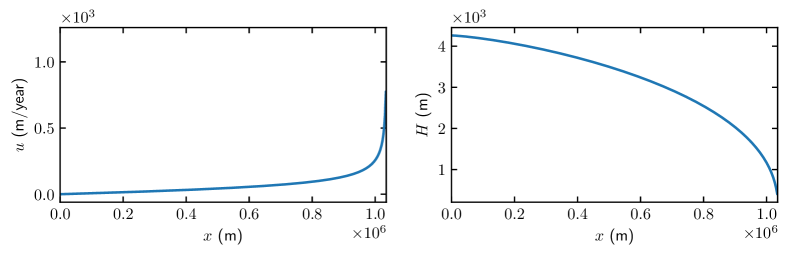
Figure 3: The analytical solutions $u(x)$ and $H(x)$ in (34) for a grounded ice in $[0,x_{GL}]$.

3.2.3 The adjoint steady state solution with $F_{u}\neq 0$

The analytical solution to (LABEL:eq:SSAadjsimp) is derived in Appendices C to D assuming that $b_{x}$ is small such that $b_{x}\ll H_{x}$ and $a$ and $C$ are constants. The expressions for $\psi$ and $v$ are found in (81)-(84). When $u$ is observed at $x_{\ast}$, then $\mathcal{F}$ and $F(u,h)$ satisfy

$$\mathcal{F}=\int_{0}^{L}u(x)\delta(x-x_{*})\,\text{d}x=u_{\ast},\;F_{u}=\delta(x-x_{*}),\;F_{h}=0,$$

and the adjoint solutions are

$$\begin{array}[]{rll}\psi(x)&=\displaystyle{\frac{Ca^{m}x_{*}}{\rho gH_{*}^{m+3}}\left(x_{GL}^{m}-x^{m}\right)},\;x_{\ast}<x\leq x_{GL},\\ \psi(x)&=\displaystyle{-\frac{1}{H_{\ast}}+\frac{Ca^{m}x_{*}}{\rho gH_{*}^{m+3}}\left(x_{GL}^{m}-x_{\ast}^{m}\right)},\;0\leq x<x_{\ast},\\ v(x)&=\displaystyle{\frac{ax_{*}}{\rho gH_{*}^{m+3}}H^{m}},\;x_{\ast}<x\leq x_{GL},\\ v(x)&=0,\;0\leq x<x_{\ast},\end{array}$$ (35)

with discontinuities at the observation point $x_{\ast}$ in $\psi(x)$ and $v(x)$. The analytical solutions $\psi(x)$ and $v(x)$ of the ice sheet in Fig. 3 at different $x_{\ast}$ positions are shown in the left panels of Fig. 4 and Fig. 5. In all figures, $m=1$ in the friction model. In Fig. 4 and subsequent figures, a Dirac term $\alpha\delta$ is plotted on a grid with grid size $\Delta x$ as a triangle with base $2\Delta x$ and height $\alpha/\Delta x$ such that the integral over the triangle is $\alpha$. The derivative $\alpha\delta^{\prime}$ is plotted as a peak $\alpha/\Delta x^{2}$ followed by $-\alpha/\Delta x^{2}$. As in Sect. 3.1.3 for the FS model, $\psi$ can be small in SSA when $\mathbf{u}$ is observed compared to observations of $h$ (cf. left and right panels of Fig. 4).

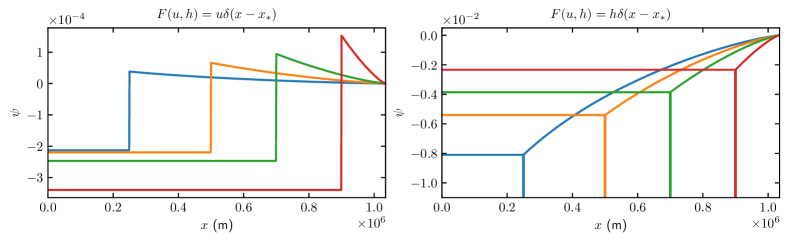
Figure 4: The analytical solutions of $\psi$ in (LABEL:eq:SSAadjsimp) of the observations of $u$ (left panel) and $h$ (right panel) at different locations $x_{\ast}=0.25\times 10^{6},0.5\times 10^{6},0.7\times 10^{6}$ and $0.9\times 10^{6}$ m (blue, orange, green and red).

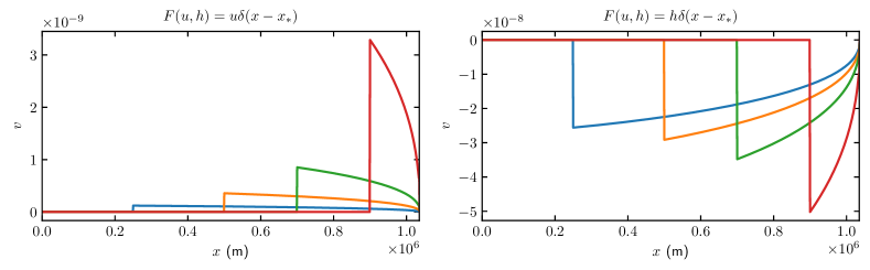
Figure 5: The analytical solutions of $v$ in (LABEL:eq:SSAadjsimp) of the observations of $u$ (left panel) and $h$ (right panel) at different locations $x_{\ast}=0.25\times 10^{6},0.5\times 10^{6},0.7\times 10^{6}$ and $0.9\times 10^{6}$ m (blue, orange, green and red).

The perturbation of the Lagrangian in (31) is derived in (85)-(86) in Appendix D

$$\begin{array}[]{lll}\displaystyle{\delta u_{\ast}}&=\delta\mathcal{L}=\displaystyle{\int_{0}^{x_{GL}}(\psi_{x}u+v_{x}\eta u_{x}+v\rho gh_{x})\,\delta b-vu^{m}\,\delta C\,\,\text{d}x}\\ &=\displaystyle{\int_{x_{\ast}^{-}}^{x_{GL}}\frac{ax_{\ast}{H^{m}}}{H^{m+3}_{*}}\left[(m+1)H_{x}\mathcal{H}(x-x_{\ast})+H\delta(x-x_{\ast})\right]\,\delta b-\frac{ax_{\ast}(ax)^{m}}{\rho gH_{*}^{m+3}}\,\delta C\,\,\text{d}x}\\ &=\displaystyle{\frac{u_{\ast}\delta b_{\ast}}{H_{\ast}}-\frac{u_{\ast}}{\rho gH_{\ast}^{m+2}}\int_{x_{\ast}}^{x_{GL}}C(ax)^{m}\left((m+1)\frac{\delta b}{H}+\frac{\delta C}{C}\right)\,\,\text{d}x},\end{array}$$ (36)

or scaled with $u_{\ast}$

$$\begin{array}[]{lll}\displaystyle{\frac{\delta u_{\ast}}{u_{\ast}}}=\displaystyle{\frac{\delta b_{\ast}}{H_{\ast}}-\frac{1}{\rho gH_{\ast}^{m+2}}\int_{x_{\ast}}^{x_{GL}}C(ax)^{m}\left((m+1)\frac{\delta b}{H}+\frac{\delta C}{C}\right)\,\,\text{d}x}.\end{array}$$ (37)

The Heaviside step function is denoted by $\mathcal{H}(x)$ in (36). The weights with respect to $\delta C$ and $\delta b$ in (36) are shown in the left panels of Fig. 6 and Fig. 7 for the same ice sheet geometry as in Fig. 3.

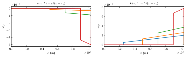
Figure 6: The analytical solution of the weights $w_{C}=-vu^{m}$ on $\delta C$ in (31) for $u$ (left panel) and $h$ (right panel) observed at $x_{\ast}=0.25\times 10^{6},0.5\times 10^{6},0.7\times 10^{6}$ and $0.9\times 10^{6}$ m (blue, orange, green and red).

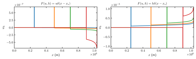
Figure 7: The analytical solution of weights $w_{b}=\psi_{x}u+v_{x}\eta u_{x}+v\rho gh_{x}$ on $\delta b$ in (31) for $u$ (left panel) and $h$ (right panel) observed at $x_{\ast}=0.25\times 10^{6},0.5\times 10^{6},0.7\times 10^{6}$ and $0.9\times 10^{6}$ m (blue, orange, green and red).

The following conclusions can be drawn from (36) and (37):

1. The weight in front of $\delta C$ increases when $x_{\ast}\rightarrow x_{GL}$. This is an effect of the increasing velocity $u_{\ast}$ and the decreasing thickness $H_{\ast}$, see Fig. 3. Therefore, a perturbation $\delta C$ with support in $[x_{\ast},x_{GL}]$ will cause larger perturbations at the surface the closer $x_{\ast}$ is to $x_{GL}$ and the closer $\delta C(x)$ is to $x_{GL}$.

2. If $\delta b_{\ast}=0$, i.e. the topography is unperturbed at the base below the observation point, then the contribution of $\delta b$ in $(x_{\ast},x_{GL}]$ cannot be separated from the contribution of $\delta C$ in (37).

3. The change in $u_{\ast}$ due to $\delta b$ in (36) is simplified if $H_{x}\ll H$. Then $\delta u_{\ast}\approx u_{\ast}\delta b_{\ast}/H_{\ast}$ and the main effect on $u_{\ast}$ from the perturbation $\delta b$ is localized at each $x_{\ast}$.

4. The perturbation in $u$ is very sensitive to $H_{\ast}$ due to the factor $u_{\ast}/H_{\ast}^{m+2}\propto 1/H_{\ast}^{m+3}$ in (36) when $x_{\ast}$ is moving downstream.

5. The relation between the two terms in (36) is estimated in a case when $\delta C=0$ and $\delta b/H$ is constant in $[x_{\ast},x_{GL}]$. Let $x_{\ast}=0.9\cdot 10^{6}$ and $x_{GL}=1.2\cdot 10^{6}$. Then $u_{\ast}\approx 130$ in Fig. 3. The factor multiplying $\delta b/H$ in the integral is by the left panel in Fig. 7 approximately ${\rm weight}\times{\rm interval}\;{\rm length}\times H\approx 150$. The contribution by the two terms is about the same but with opposite signs. The integral term is reduced if the interval where $\delta C\neq 0$ is shorter.

6. With an unperturbed topography, let the perturbation of the friction coefficient be a constant $\delta C_{0}\neq 0$ in $[x_{0},x_{1}]\in[x_{\ast},x_{GL}]$ resulting in a perturbation of the velocity. Evaluate the integral in (36) to obtain

   $${\delta u_{\ast}}=\displaystyle{-\frac{u_{\ast}}{\rho gH_{\ast}^{m+2}}\int_{x_{0}}^{x_{1}}(ax)^{m}\delta C_{0}\,\,\text{d}x=-\frac{a^{m}u_{\ast}}{(m+1)\rho gH_{\ast}^{m+2}}(x_{1}^{m+1}-x_{0}^{m+1})\delta C_{0}}.$$ (38)

   The same $\delta u_{\ast}$ is observed with a constant perturbation in $[x_{2},x_{3}]\in[x_{\ast},x_{GL}]$ with the amplitude $\delta C_{0}(x_{1}^{m+1}-x_{0}^{m+1})/(x_{3}^{m+1}-x_{2}^{m+1})$. Different $\delta C$ can give rise to the same observation $\delta u_{\ast}$. This holds true also for different $\delta b$ when $\delta b_{\ast}=0$. Inference of $\delta C$ or $\delta b$ from surface data requires more observation points than one.

7. Perturb $C$ by $\delta C=\epsilon\cos(kx/x_{GL})$ in (36) for some wave number $k$ and amplitude $\epsilon$ and let $\delta b=0$ and $m=1$. Then

   $$\begin{array}[]{lll}\delta u_{\ast}&=\displaystyle{-\int_{x_{\ast}}^{x_{GL}}\epsilon\frac{a^{2}x_{*}}{\rho gH_{*}^{4}}x\cos\left(\frac{kx}{x_{GL}}\right)\,\,\text{d}x}\\ &=\displaystyle{-\epsilon\frac{a^{2}x_{*}}{\rho gH_{*}^{4}}\frac{x_{GL}^{2}}{k}\left(\sin(k)-\frac{x_{\ast}}{x_{GL}}\sin\left(\frac{kx_{\ast}}{x_{GL}}\right)+\frac{1}{k}\left(\cos(k)-\cos\left(\frac{kx_{\ast}}{x_{GL}}\right)\right)\right)}.\end{array}$$ (39)

   When $k$ grows at the ice base, the amplitude of the perturbation at the ice surface decays as $1/k$. The effect of high wave number perturbations of $C$ will be difficult to observe at the top of the ice. When $k$ vanishes, then $\delta u_{\ast}$ tends to constant.

8. If $\delta C=0$ and $b$ is perturbed by $\delta b=\epsilon\cos(kx/x_{GL})$, then any perturbation at $x_{\ast}$ is propagated to the surface by the first term on the right hand side of (36). The integral term will behave in the same way as in (39).

Let the friction coefficient $C$ be perturbed by a constant $\delta C$ in $[0,x_{GL}]$ and take $\delta b=0$. Then it follows from (36) that

$$\delta u_{*}=\delta C\int_{x_{\ast}}^{x_{GL}}-vu^{m}\,\text{d}x=\frac{a^{m+1}x_{\ast}(x_{*}^{m+1}-x_{GL}^{m+1})}{(m+1)\rho gH_{*}^{m+3}}\;\delta C.$$ (40)

Computing the derivative of $u(x,C)$ with respect to $C$ in the explicit expression in (34) at $x_{*}$ yields the same result.

The sensitivity of surface data to changes in $b$ and $C$ is estimated in (Gudmundsson and Raymond 2008) with a linearized model and Fourier analysis. The conclusion is that differences of short wavelength in the bedrock topography cannot be observed at the surface. Only differences with long wavelength in the friction coefficient propagate to the top of the ice. This is in agreement with (36) and (37) and conclusions 7 and 8 above.

3.2.4 The adjoint steady state solution with $F_{h}\neq 0$

In the case when $h$ is observed at $x_{\ast}$ and $F_{u}=0$ and $F_{h}=\delta(x-x_{\ast})$, the expressions for $\psi$ and $v$ are

$$\begin{array}[]{rll}\psi(x)&=\displaystyle{-\frac{Ca^{m-1}}{\rho gH_{*}^{m+1}}\left(x_{GL}^{m}-x^{m}\right)},\;x_{\ast}<x\leq x_{GL},\\ \psi(x)&=\displaystyle{-\frac{Ca^{m-1}}{\rho gH_{*}^{m+1}}\left(x_{GL}^{m}-x_{\ast}^{m}\right)},\;0\leq x<x_{\ast},\\ v(x)&=\displaystyle{-\frac{H^{m}}{\rho gH_{*}^{m+1}}},\;x_{\ast}<x\leq x_{GL},\\ v(x)&=0,\;0\leq x<x_{\ast}.\end{array}$$ (41)

There is a discontinuity at the observation point $x_{\ast}$ in $v(x)$, see Fig. 5, but $\psi(x)$ is continuous in the solution of (LABEL:eq:SSAadjsimp). Actually, $\psi(x)\sim-\delta(x-x_{\ast})$ in the neighborhood of $x_{\ast}$ due to the second derivative term $(\frac{1}{n}\eta Hv_{x})_{x}$ which is neglected in the simplified equation (LABEL:eq:SSAadjsimp) but is of importance at $x_{\ast}$. A correction $\hat{\psi}$ of $\psi$ at $x_{\ast}$ is therefore introduced to satisfy $\left(\frac{1}{n}\eta Hv_{x}\right)_{x}-H\hat{\psi}_{x}=0$. With $v_{x}(x_{\ast})=-\delta(x-x_{\ast})/(\rho gH_{\ast})$, the correction is $\hat{\psi}(x)=-\delta(x-x_{\ast})\eta_{\ast}/(n\rho gH_{\ast})$. The solution $\psi$ is corrected at each $x_{\ast}$ in Fig. 4 with $\hat{\psi}$. The perturbation in $h$ is as in (36) with $\psi$ and $v$ in (41) and the additional term $\hat{\psi}$

$$\begin{array}[]{lll}\displaystyle{\frac{\delta h_{\ast}}{H_{\ast}}}&=\displaystyle{\int_{x_{\ast}^{-}}^{x_{GL}}-\frac{u\eta_{\ast}}{n\rho gH_{\ast}^{2}}\delta_{x}(x-x_{\ast})\delta b}\,\,\text{d}x+\displaystyle{\int_{x_{\ast}}^{x_{GL}}\frac{C(ax)^{m}}{\rho gH^{m+2}_{*}}\left((m+1)\frac{\delta b}{H}+\frac{\delta C}{C}\right)\,\,\text{d}x}\\ &=\displaystyle{\frac{a\eta_{\ast}}{n\rho gH_{\ast}^{2}}\left(x\frac{\delta b}{H}\right)_{x}(x_{\ast})+{\frac{1}{\rho gH^{m+2}_{*}}\int_{x_{\ast}}^{x_{GL}}C(ax)^{m}\left((m+1)\frac{\delta b}{H}+\frac{\delta C}{C}\right)\,\,\text{d}x}},\end{array}$$ (42)

where $a(x\delta b/H)_{x}(x_{\ast})=(u\delta b)_{x}(x_{\ast})$ represents the $x$-derivative of $u\delta b$ evaluated at $x_{\ast}$. When $\delta b=0$ then $\delta u_{\ast}$ in (37) and $\delta h_{\ast}=\delta H_{\ast}$ in (42) satisfy $\delta u_{\ast}H_{\ast}=-\delta H_{\ast}u_{\ast}$ as in the integrated form of the advection equation in (LABEL:eq:SSAforwsimp) and in (68).

The contribution from the integrals in (37) and (42) is identical except for the sign (see also Fig. 6). The first term in (37) depends on $\delta b/H$ and the first term in (42) depends on the derivative of $x\delta b/H$. Because of these similarities, the conclusions 1, 2, 6, 7, and 8 from (36) and (37) for $\delta u_{\ast}$ are valid also for $\delta h_{\ast}$ in (42). The change in $h$ caused by $\delta C$ is less sensitive to $H_{\ast}$ than the change in $u$ since the factor multiplying the integral is proportional to $1/H_{\ast}^{m+1}$.

If $u\delta b=ax\delta b/H$ is constant, then $\delta h$ is determined by the continuous weight in $x\in[x_{\ast},x_{GL}]$ in Fig. 7 which has a shape similar to the $\delta C$ weight in Fig. 6. A perturbation of $b$ at the base is directly visible locally in $u$ at the surface while the effect of $\delta C$ is non-local in (42).

3.2.5 The time dependent adjoint solution

The time dependent adjoint equation (LABEL:eq:SSAadj) is solved numerically for the MISMIP test case in Sect. 3.2.2. Starting from the steady state solution, the friction coefficient $C$ has a seasonal variation in the forward equation (LABEL:eq:SSAforw), such that $C(x,t)=C_{0}(1+\kappa\cos(2\pi t)),\;0<\kappa<1$. Apparently, $C$ has its highest value at $t=n,\;n=0,1,2,\ldots$, i.e. the winter, and its lowest value at $t=n+1/2$, i.e. the summer. The period of the seasonal variation is 1 a and the beginning of each year is in the winter.

The amplitude of the pertubation is set to $\kappa=0.5$ and the forward equation (LABEL:eq:SSAforw) is solved for 11 years. Observations on $u$ and $h$ are taken at $x_{*}=9\times 10^{5}$ m for 0.1 a in the four seasons of the tenth year, e.g., in the summer $(t=9.5)$, the fall $(t_{\ast}=9.75)$, the winter $(t=10)$, and the spring $(t=10.25)$. The adjoint equations (LABEL:eq:SSAadj) are solved from the observation points backward in time, respectively, as in Figs. 8 and 9. According to a convergence test, the time step is chosen to be $0.01$ a and the spatial resolution is $10^{3}~{}$m.

The adjoint weights $w_{C}$ and $w_{b}$, as defined in (31), are shown in Fig. 8 for the observations on $u$ and $h$ at $x_{*}=9\times 10^{5}$ m in the four seasons. The time axis in the figure starts from the steady state solution and follows the time direction in the forward problem. As expected, most of the weights in space and time are negligible. Therefore, we take a snapshot with the width of $10^{5}$ m in space around $x_{\ast}$. Only $\delta C$ and $\delta b$ in a narrow interval around $x_{\ast}$ for $t$ in $[0,t_{\ast}]$ have an influence on $\delta u_{\ast}$ and $\delta h_{\ast}$, see Fig. 8. A perturbation at the base is propagated to the $x_{\ast}$ position on the surface but with a possible delay in time.

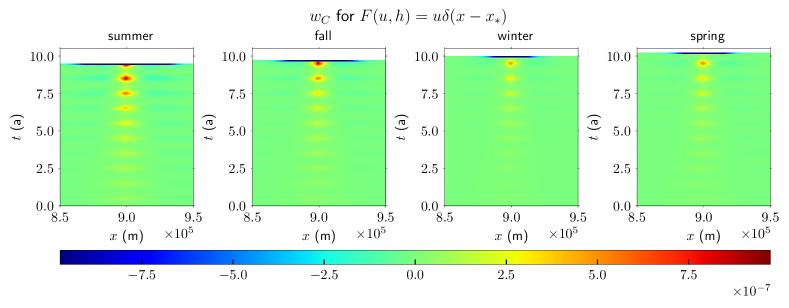
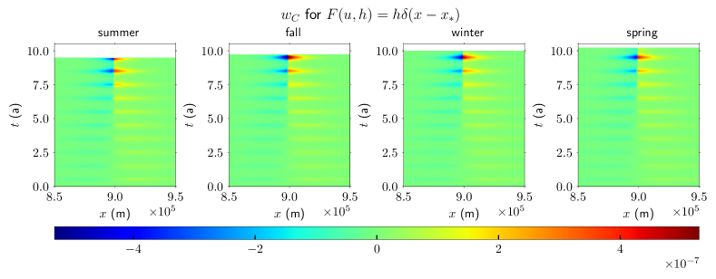
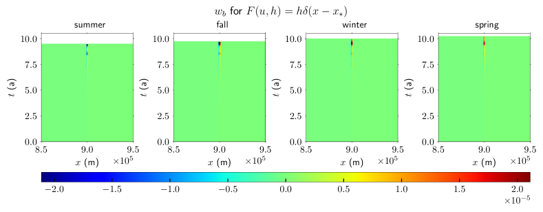
Figure 8: The adjoint weights for the observations at $x_{*}=9\times 10^{5}$ m of the four seasons. The first row: $w_{C}$ for the observation of $u$. The second row: $w_{b}$ for the observation of $u$. The third row: $w_{C}$ for the observation of $h$. The last row: $w_{b}$ for the observation of $h$.

The temporal variations of the adjoint weights at $x_{\ast}$ in Fig. 8 are shown in Fig. 9 for the four seasons with four different colors. As expected, the weights vanish when $t>t_{\ast}$. In the left panels of Fig. 9, the perturbations $\delta C_{\ast}$ and $\delta b_{\ast}$ have a direct effect on $\delta u_{\ast}$ at $t_{\ast}$, where $w_{C}(x_{\ast})$ and $w_{b}(x_{\ast})$ are both negative. The same conclusion is valid for $\delta u_{1\ast}$ computed from the FS equations (18) in Sect. 3.1.1. A change in $\delta C_{\ast}$ at the base is observed immediately as a change in $u$ at the surface. The effect of $\delta C$ on $\delta u_{\ast}$ for $t<t_{\ast}$ is weak in the upper left panel of Fig. 9. The largest effect of $\delta C$ on $\delta u_{\ast}$ and $\delta h_{\ast}$ appears in the summer when $C$ is small, as the blue lines in the left panels.

However, when $h$ is observed, the effect of $\delta C_{\ast}$ and $\delta b_{\ast}$ are not visible directly because $w_{C\ast}\approx 0$ and $w_{b\ast}\approx 0$ in the right panels of Fig. 9. Additionally, the effect of $\delta C$ and $\delta b$ is difficult to be separated, since the weight $w_{b}(x_{\ast})$ has the similar shape as $w_{C}(x_{\ast})$. The largest effect on $\delta h_{\ast}$ is from $\delta C$ in the summer due to the peaks as in the upper right panel. For the same $\delta C$, the largest $\delta h_{\ast}$ is observed in the fall (orange), then the second largest $\delta h_{\ast}$ is in the winter (green) followed by the spring observation (red). If $\delta h_{\ast}$ is observed in the fall and the time dependency is ignored, then the wrong conclusion is drawn that $\delta C$ in the fall has the strongest effect. There is a delay in time between the perturbation and the observation of the effect.

A reference adjoint solution observed during the fall season ($t_{\ast}=9.75$) with $\kappa=0$ in the forward equations is shown in the black dashed lines in Fig. 9. The weight $w_{b}$ for a constant $b$ in time is well approximated by $\exp(-(T-t)/\tau)$ with $\tau=1.4$ a. For the weight $w_{C}$, the same exponential function holds, but the constant $\tau=1.8$ a for the observation of $h_{\ast}$ and $\tau=2.2$ a for the $u_{\ast}$ case. Suppose that the temporal perturbation is oscillatory $\delta C_{0}\cos(2\pi ft)$ with frequency $f$. Then perturbation in $h$ at $t=t_{\ast}$ is

$$\begin{array}[]{rll}\delta h&=\displaystyle{\int_{0}^{T}\exp(-(T-t)/\tau)\delta C_{0}\cos(2\pi ft)\,\text{d}t}\\ &=\left(\displaystyle{\frac{\cos(2\pi fT)+2\pi\tau f\sin(2\pi fT)-e^{-T/\tau}}{4\pi^{2}\tau f^{2}+\tau^{-1}}}\right)\delta C_{0},\end{array}$$ (43)

cf. (39). With a high frequency (diurnal), $f\gg 1$, then $\delta h\propto 1/f$ and high frequency perturbations are damped efficiently. If the frequency is low (decennial), $f\ll 1$, then $\delta h\propto\tau$ and the change in $h$ is insensitive to the frequency. The same conclusions hold true for $\delta b$ where decennial variations seem more realistic.

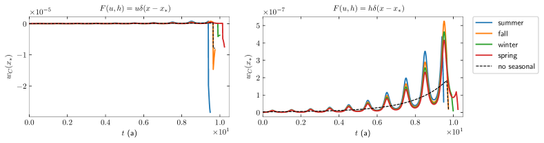
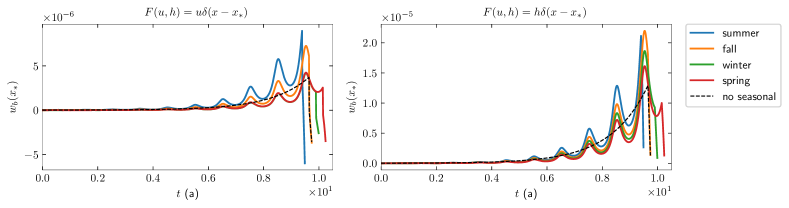
Figure 9: The adjoint weights for the observations of $u$ and $h$ at $x_{\ast}$ in the four seasons of the tenth year with seasonal varying friction coefficient. The black dashed line is a reference solution without seasonal variations which is observed at $t=9.75$.

4 Conclusions

The sensitivity of the flow of ice to basal conditions is analyzed for time dependent and steady state solutions of the FS and SSA equations including the advection equation for the height. Perturbations at the base of the ice are introduced in the friction coefficient $C$ and the topography $b$. The analysis relies on the adjoint equations of the FS and SSA stress and advection equations. The adjoint FS and SSA equations follow from the Lagrangians of the forward FS and SSA equations.

The adjoint equations are derived for observations of the velocity $\mathbf{u}$ and height $h$ at the top surface of the ice. The adjoint height equation in the FS model is solved analytically for a two dimensional vertical ice. The relation between the inverse problem to find parameters from data and the sensitivity problem is established. The same adjoint equations are solved in the inverse problem but with other forcing functions.

If the perturbations in the basal conditions are time dependent then time cannot be ignored in the inversion. It is necessary to include the adjoint height equation if $h$ is observed. The wrong conclusions may be drawn with only static snapshots for both the FS and the SSA model. If $\mathbf{u}$ is observed then the contribution of the solution of the adjoint height equation is small and it is sufficient to solve only the adjoint stress equation as is the case in many articles on inversion e.g. (Gillet-Chaulet et al. 2016, Isaac et al. 2015, Petra et al. 2012).

The adjoint equations of the FS and SSA models are similar and the analytical solutions based on the SSA equations for a two dimensional vertical ice show that the sensitivity grows as the observation point $x_{\ast}$ is approaching the grounding line separating the grounded and the floating parts of the ice. The reason is that the velocity increases and the thickness of the ice decreases.

In the steady state solution of SSA, there is a non-local effect of a perturbation $\delta C$ in $C$ in the sense that $\delta C(x)$ affects both $u(x_{\ast})$ and $h(x_{\ast})$ even if $x\neq x_{\ast}$, but $\delta b$ has a strong local effect concentrated at $x_{\ast}$. Nevertheless, the shapes of the two sensitivity functions for $\delta b$ and $\delta C$ are very similar except for the neighborhood of $x_{\ast}$. It is possible to separate the effect of $\delta b$ and $\delta C$ in the steady state SSA model thanks to the localized influence of $\delta b$ in $\delta u$ and $\delta h$. The same effect on $\delta u$ and $\delta h$ at one observation point can be achieved by different $\delta C$ and $\delta b$. Perturbations in $C$ at the base observed in $u$ at the surface are damped inversely proportional to the wavenumber of $\delta C$ thus making high wavenumber perturbations difficult to register at the top.

In the time dependent solution of SSA, the strongest impact of a perturbation at $x_{\ast}$ is made at $x_{\ast}$ at the surface possibly with a time delay. There is a local effect of $\delta C$ and $\delta b$ at $(x_{\ast},t_{\ast})$ on $u_{\ast}$ but not on $h_{\ast}$ where perturbations are caused by $\delta C(x,t)$ and $\delta b(x,t)$ with $t<t_{\ast}$. There is a time delay when a perturbation at the ice base is visible at the surface in $h$ but in $u$ it is observed immediately. As in the steady state, the same effect on $\delta u$ and $\delta h$ can be achieved by different $\delta C$ and $\delta b$. The higher the frequency of the perturbation is the more it is damped at the surface, but perturbations of low frequency reach the upper surface.

The numerical results in (Cheng and Lötstedt 2019) confirm the conclusions here and are in good agreement with the analytical solutions.

Appendix A Derivation of the adjoint equations

A.1 Adjoint viscosity and friction in SSA

The adjoint viscosity $\tilde{\boldsymbol{\eta}}(\mathbf{u})$ in SSA in (14) is derived as follows. The SSA viscosity for $\mathbf{u}$ and $\mathbf{u}+\delta\mathbf{u}$ is

$$\begin{array}[]{ll}\eta(\mathbf{u}+\delta\mathbf{u})\\ \approx\eta(\mathbf{u})\left(1+\frac{1-n}{2n}\frac{(2u_{1x}+u_{2y})\delta u_{1x}+\frac{1}{2}(u_{1y}+u_{2x})\delta u_{2x}+(2u_{2y}+u_{1x})\delta u_{2y}+\frac{1}{2}(u_{1y}+u_{2x})\delta u_{1y}}{\hat{\eta}}\right).\end{array}$$ (44)

Determine $\mathcal{B}(\mathbf{u})$ such that

$$\varrho(\mathbf{u},\delta\mathbf{u})\mathbf{B}(\mathbf{u})=\mathcal{B}(\mathbf{u})\star\mathbf{B}(\delta\mathbf{u}).$$

First note that

$$\begin{array}[]{ll}\mathbf{B}(\mathbf{u}):\mathbf{D}(\delta\mathbf{u})=(\mathbf{D}(\mathbf{u})+\nabla\cdot\mathbf{u}\mathbf{I}):\mathbf{D}(\delta\mathbf{u})=\mathbf{D}(\mathbf{u}):\mathbf{D}(\delta\mathbf{u})+(\nabla\cdot\mathbf{u})(\nabla\cdot\delta\mathbf{u})\\ =\mathbf{D}(\mathbf{u}):(\mathbf{B}(\delta\mathbf{u})-\nabla\cdot\delta\mathbf{u}\mathbf{I})+(\nabla\cdot\mathbf{u})(\nabla\cdot\delta\mathbf{u})=\mathbf{D}(\mathbf{u}):\mathbf{B}(\delta\mathbf{u}).\end{array}$$

Then use the $\star$ operator in (16) to define $\mathcal{B}$

$$\begin{array}[]{rll}\frac{1-n}{2n\hat{\eta}}\sum_{kl}B_{kl}(\mathbf{u})D_{kl}(\delta\mathbf{u})B_{ij}(\mathbf{u})&=\frac{1-n}{2n\hat{\eta}}\sum_{kl}D_{kl}(\mathbf{u})B_{kl}(\delta\mathbf{u})B_{ij}(\mathbf{u})\\ &=\sum_{kl}\mathcal{B}_{ijkl}(\mathbf{u})D_{kl}(\delta\mathbf{u})=(\mathcal{B}\star D)_{ij}.\end{array}$$

Thus, let

$$\mathcal{B}_{ijkl}=\frac{1-n}{2n\hat{\eta}}B_{ij}(\mathbf{u})D_{kl}(\mathbf{u}),\quad\tilde{\eta}_{ijkl}(\mathbf{u})=\eta(\mathbf{u})(\mathcal{I}_{ijkl}+\mathcal{B}_{ijkl}(\mathbf{u})),$$

or in tensor form

$$\mathcal{B}=\frac{1-n}{n\mathbf{B}(\mathbf{u}):\mathbf{D}(\mathbf{u})}\mathbf{B}(\mathbf{u})\otimes\mathbf{D}(\mathbf{u}),\quad\tilde{\boldsymbol{\eta}}(\mathbf{u})=\eta(\mathbf{u})\left(\mathcal{I}+\mathcal{B}\right).$$ (45)

Replacing $\mathbf{B}$ in (45) by $\mathbf{D}$ we obtain the adjoint FS viscosity in (14).

The adjoint friction in SSA in $\omega$ and at $\gamma_{g}$ in (LABEL:eq:SSAadj3D) with a Weertman law is derived as in the adjoint FS equations (LABEL:eq:FSadj) and (14). Then in $\omega$ with $\boldsymbol{\xi}=\mathbf{u},\boldsymbol{\zeta}=\mathbf{v},c=C,\mathbf{F}=\mathbf{F}_{\omega}$, and at $\gamma_{g}$ with $\boldsymbol{\xi}=\mathbf{t}\cdot\mathbf{u},\boldsymbol{\zeta}=\mathbf{t}\cdot\mathbf{v},c=C_{\gamma},f=f_{\gamma},\mathbf{F}=F_{\gamma},$ we arrive at the adjoint friction term $cf(\boldsymbol{\xi})\left(\mathbf{I}+\mathbf{F}(\boldsymbol{\xi})\right)\boldsymbol{\zeta}$ where

$$\mathbf{F}(\boldsymbol{\xi})=\frac{m-1}{\boldsymbol{\xi}\cdot\boldsymbol{\xi}}\boldsymbol{\xi}\otimes\boldsymbol{\xi}.$$ (46)

A.2 Adjoint equations in SSA

The Lagrangian for the SSA equations is with the adjoint variables $\psi,\mathbf{v},q$

$$\begin{array}[]{rll}&\mathcal{L}(\mathbf{u},h;\mathbf{v},\psi;b,C_{\gamma},C)=\int_{0}^{T}\int_{\omega}F(\mathbf{u},h)+\psi(h_{t}+\nabla\cdot(\mathbf{u}H)-a)\,\text{d}\mathbf{x}\,\text{d}t\\ &+\int_{0}^{T}\int_{\omega}\mathbf{v}\cdot\nabla\cdot(2H\eta\mathbf{B}(\mathbf{u}))-Cf(\mathbf{u})\mathbf{v}\cdot\mathbf{u}-\rho gH\mathbf{v}\cdot\nabla h\,\,\text{d}\mathbf{x}\,\text{d}t\\ &=\int_{0}^{T}\int_{\omega}F(\mathbf{u},h)+\psi(h_{t}+\nabla\cdot(\mathbf{u}H)-a)\,\text{d}\mathbf{x}\,\text{d}t\\ &+\int_{0}^{T}\int_{\omega}-2H\eta(\mathbf{u})(\mathbf{D}(\mathbf{v}):\mathbf{D}(\mathbf{u})+\nabla\cdot\mathbf{u}\nabla\cdot\mathbf{v})\\ &-Cf(\mathbf{u})\mathbf{v}\cdot\mathbf{u}-\rho gH\mathbf{v}\cdot\nabla h\,\,\text{d}\mathbf{x}\,\text{d}t-\int_{0}^{T}\int_{\gamma_{g}}C_{\gamma}f_{\gamma}(\mathbf{t}\cdot\mathbf{u})\mathbf{t}\cdot\mathbf{u}\,\mathbf{t}\cdot\mathbf{v}\,\text{d}s\,\text{d}t\end{array}$$ (47)

after partial integration and using the boundary conditions. The perturbed SSA Lagrangian is split into the unperturbed Lagrangian and three integrals

$$\begin{array}[]{lll}\mathcal{L}(\mathbf{u}+\delta\mathbf{u},h+\delta h;\mathbf{v}+\delta\mathbf{v},\psi+\delta\psi;b+\delta b,C_{\gamma}+\delta C_{\gamma},C+\delta C)\\ =\int_{0}^{T}\int_{\omega}F(\mathbf{u}+\delta\mathbf{u},h+\delta h)\\ +\int_{0}^{T}\int_{\omega}(\psi+\delta\psi)(h_{t}+\delta h_{t}+\nabla\cdot\left((\mathbf{u}+\delta\mathbf{u})(H+\delta H)\right)-a)\,\text{d}\mathbf{x}\,\text{d}t\\ +\int_{0}^{T}\int_{\omega}-2(H+\delta H)\eta(\mathbf{u}+\delta\mathbf{u})\mathbf{D}(\mathbf{v}+\delta\mathbf{v}):\mathbf{B}(\mathbf{u}+\delta\mathbf{u})\\ -(C+\delta C)f(\mathbf{u}+\delta\mathbf{u})(\mathbf{u}+\delta\mathbf{u})\cdot(\mathbf{v}+\delta\mathbf{v})\\ -\rho g(H+\delta H)\nabla(h+\delta h)\cdot(\mathbf{v}+\delta\mathbf{v})\,\,\text{d}\mathbf{x}\,\text{d}t\\ -\int_{0}^{T}\int_{\gamma_{g}}(C_{\gamma}+\delta C_{\gamma})f_{\gamma}(\mathbf{t}\cdot(\mathbf{u}+\delta\mathbf{u}))\mathbf{t}\cdot(\mathbf{u}+\delta\mathbf{u})\,\mathbf{t}\cdot(\mathbf{v}+\delta\mathbf{v})\,\text{d}s\,\text{d}t\\ =\mathcal{L}(\mathbf{u},h;\mathbf{v},\psi;b,C_{\gamma},C)+I_{1}+I_{2}+I_{3}.\end{array}$$ (48)

The perturbation in $\mathcal{L}$ is

$$\delta\mathcal{L}=I_{1}+I_{2}+I_{3}.$$ (49)

Terms of order two or more in $\delta\mathcal{L}$ are neglected. Then the first term in $\delta\mathcal{L}$ satisfies

$$\begin{array}[]{rll}I_{1}&=\int_{0}^{T}\int_{\omega}F(\mathbf{u}+\delta\mathbf{u},h+\delta h)-F(\mathbf{u},h)\,\text{d}\mathbf{x}\,\text{d}t\\ &=\int_{0}^{T}\int_{\omega}F_{\mathbf{u}}\delta\mathbf{u}+F_{h}\delta h\,\text{d}\mathbf{x}\,\text{d}t.\end{array}$$ (50)

Using partial integration, Gauss’ formula, and the initial and boundary conditions on $\mathbf{u}$ and $H$ and $\psi(\mathbf{x},T)=0,\mathbf{x}\in\omega,$ and $\psi(\mathbf{x},t)=0,\;\mathbf{x}\in\gamma_{w},$ in the second integral we have

$$\begin{array}[]{rll}I_{2}&=&\int_{0}^{T}\int_{\omega}\delta\psi(h_{t}+\nabla\cdot(\mathbf{u}H)-a)\\ &&+\psi(\delta h_{t}+\nabla\cdot(\delta\mathbf{u}H)+\nabla\cdot(\mathbf{u}\delta H))\,\text{d}\mathbf{x}\,\text{d}t\\ &=&\int_{0}^{T}\int_{\omega}\delta\psi(h_{t}+\nabla\cdot(\mathbf{u}H)-a)\,\text{d}\mathbf{x}\,\text{d}t\\ &&+\int_{0}^{T}\int_{\omega}-\psi_{t}\delta h-H\nabla\psi\cdot\delta\mathbf{u}-\nabla\psi\cdot\mathbf{u}\delta H\,\text{d}\mathbf{x}\,\text{d}t.\end{array}$$ (51)

The first integral after the second equality vanishes since $h$ is a weak solution and $I_{2}$ is

$$\begin{array}[]{rll}I_{2}=\int_{0}^{T}\int_{\omega}-(\psi_{t}+\mathbf{u}\cdot\nabla\psi)\delta h-H\nabla\psi\cdot\delta\mathbf{u}+\mathbf{u}\cdot\nabla\psi\delta b\,\text{d}\mathbf{x}\,\text{d}t.\end{array}$$ (52)

Using the weak solution of (LABEL:eq:SSAforw3D), the adjoint viscosity (27), (45), the friction coefficient (46), Gauss’ formula, the boundary conditions, and neglecting the second order terms, the third and fourth integrals in (48) are

$$\begin{array}[]{rll}I_{3}=&I_{31}+I_{32},\\ I_{31}=&\int_{0}^{T}\int_{\omega}-2(H+\delta H)\eta(\mathbf{u}+\delta\mathbf{u})\mathbf{D}(\mathbf{v}+\delta\mathbf{v}):\mathbf{B}(\mathbf{u}+\delta\mathbf{u})\\ &-(C+\delta C)f(\mathbf{u}+\delta\mathbf{u})(\mathbf{u}+\delta\mathbf{u})\cdot(\mathbf{v}+\delta\mathbf{v})\\ &-\rho g(H+\delta H)\nabla(h+\delta h)\cdot(\mathbf{v}+\delta\mathbf{v}))\,\,\text{d}\mathbf{x}\,\text{d}t\\ &-\int_{0}^{T}\int_{\gamma}(C_{\gamma}+\delta C_{\gamma})f_{\gamma}(\mathbf{t}\cdot(\mathbf{u}+\delta\mathbf{u}))\mathbf{t}\cdot(\mathbf{u}+\delta\mathbf{u})\,\mathbf{t}\cdot(\mathbf{v}+\delta\mathbf{v})\,\text{d}s\,\text{d}t\\ =&I_{311}+I_{312}-I_{313},\end{array}$$ (53)

where

$$\begin{array}[]{rll}I_{311}=&\int_{0}^{T}\int_{\omega}-2H\mathbf{D}(\mathbf{v}):(\eta(\mathbf{u}+\delta\mathbf{u})\mathbf{B}(\mathbf{u}+\delta\mathbf{u}))\\ &+2H\mathbf{D}(\mathbf{v}):(\eta(\mathbf{u})\mathbf{B}(\mathbf{u}))\,\text{d}\mathbf{x}\,\text{d}t\\ =&\int_{0}^{T}\int_{\omega}-2H\mathbf{D}(\mathbf{v}):(\tilde{\boldsymbol{\eta}}(\mathbf{u})\star\mathbf{B}(\delta\mathbf{u}))\,\text{d}\mathbf{x}\,\text{d}t\\ I_{312}=&\int_{0}^{T}\int_{\omega_{g}}-\delta Cf(\mathbf{u})\mathbf{u}\cdot\mathbf{v}\,\text{d}\mathbf{x}\,\text{d}t\\ &+\int_{0}^{T}\int_{\omega_{g}}-C(f(\mathbf{u}+\delta\mathbf{u})\mathbf{v}\cdot(\mathbf{u}+\delta\mathbf{u})-f(\mathbf{u})\mathbf{v}\cdot\mathbf{u})\,\text{d}\mathbf{x}\,\text{d}t\\ =&\int_{0}^{T}\int_{\omega_{g}}-\delta Cf(\mathbf{u})\mathbf{u}\cdot\mathbf{v}+Cf(\mathbf{u})(\mathbf{I}+\mathbf{F}_{\omega}(\mathbf{u}))\delta\mathbf{u}\cdot\mathbf{v}\,\text{d}\mathbf{x}\,\text{d}t\\ I_{313}=&\int_{0}^{T}\int_{\gamma_{g}}(C_{\gamma}+\delta C_{\gamma})(f_{\gamma}(\mathbf{t}\cdot(\mathbf{u}+\delta\mathbf{u}))\mathbf{t}\cdot\mathbf{v}\,\mathbf{t}\cdot(\mathbf{u}+\delta\mathbf{u})\\ &-f_{\gamma}(\mathbf{t}\cdot\mathbf{u})\mathbf{t}\cdot\mathbf{v}\,\mathbf{t}\cdot\mathbf{u})\,\text{d}s\,\text{d}t\\ =&\int_{0}^{T}\int_{\gamma_{g}}(C_{\gamma}+\delta C_{\gamma})(f_{\gamma}(\mathbf{t}\cdot\mathbf{u})\mathbf{t}\cdot\mathbf{u}\,\mathbf{t}\cdot\mathbf{v}\\ &+C_{\gamma}f_{\gamma}(\mathbf{t}\cdot\mathbf{u})(\mathbf{I}+\mathbf{F}_{\gamma}(\mathbf{t}\cdot\mathbf{u}))\mathbf{t}\cdot\delta\mathbf{u}\,\mathbf{t}\cdot\mathbf{v}\,\text{d}s\,\text{d}t\\ I_{32}=&\int_{0}^{T}\int_{\omega}-\rho gH\nabla h\cdot\mathbf{v}-2\eta\mathbf{D}(\mathbf{v}):\mathbf{B}(\mathbf{u})\delta H\\ &-\rho g\nabla h\cdot\mathbf{v}\delta H-\rho gH\mathbf{v}\cdot\nabla\delta h\,\text{d}\mathbf{x}\,\text{d}t\\ =&\int_{0}^{T}\int_{\omega}-\rho gH\nabla h\cdot\mathbf{v}-(2\eta\mathbf{D}(\mathbf{v}):\mathbf{B}(\mathbf{u})+\rho g\nabla h\cdot\mathbf{v})\delta H\\ &+\rho g\nabla\cdot(H\mathbf{v})\delta h\,\text{d}\mathbf{x}\,\text{d}t.\end{array}$$ (54)

Collecting all the terms in (50), (52), and (53), the first variation of $\mathcal{L}$ is

$$\begin{array}[]{rll}\delta\mathcal{L}&=&I_{1}+I_{2}+I_{3}\\ &=&\int_{0}^{T}\int_{\omega}F_{\mathbf{u}}\delta\mathbf{u}-2HD(\mathbf{v}):(\tilde{\boldsymbol{\eta}}(\mathbf{u})\star\mathbf{B}(\delta\mathbf{u}))-H\nabla\psi\cdot\delta\mathbf{u}\,\text{d}\mathbf{x}\,\text{d}t\\ &&-\int_{0}^{T}\int_{\omega_{g}}Cf(\mathbf{u})(\mathbf{I}+\mathbf{F}_{\omega}(\mathbf{u}))\mathbf{v}\cdot\delta\mathbf{u}\,\text{d}\mathbf{x}\,\text{d}t\\ &&-\int_{0}^{T}\int_{\gamma_{g}}C_{\gamma}f_{\gamma}(\mathbf{t}\cdot\mathbf{u})(\mathbf{I}+\mathbf{F}_{\gamma}(\mathbf{t}\cdot\mathbf{u}))\mathbf{t}\cdot\mathbf{v}\,\mathbf{t}\cdot\delta\mathbf{u}\,\text{d}s\,\text{d}t\\ &&-\int_{0}^{T}\int_{\gamma_{g}}\delta C_{\gamma}f_{\gamma}(\mathbf{t}\cdot\mathbf{u})\mathbf{t}\cdot\mathbf{u}\,\mathbf{t}\cdot\mathbf{v}\,\text{d}s\,\text{d}t\\ &&+\int_{0}^{T}\int_{\omega}(F_{h}-(\psi_{t}+\mathbf{u}\cdot\nabla\psi+2\eta\mathbf{D}(\mathbf{v}):\mathbf{B}(\mathbf{u})\\ &&-\rho g\nabla b\cdot\mathbf{v}+\rho gH\nabla\cdot\mathbf{v}))\delta h\,\text{d}\mathbf{x}\,\text{d}t\\ &&+\int_{0}^{T}\int_{\omega}-\delta Cf(\mathbf{u})\mathbf{v}\cdot\mathbf{u}\\ &&+(2\eta\mathbf{D}(\mathbf{v}):\mathbf{B}(\mathbf{u})+\rho g\nabla h\cdot\mathbf{v}+\mathbf{u}\cdot\nabla\psi)\delta b\,\text{d}\mathbf{x}\,\text{d}t.\end{array}$$ (55)

The forward solution $(\mathbf{u}^{*},p^{*},h^{*})$ and adjoint solution $(\mathbf{v}^{*},q^{*},\psi^{*})$ satisfying (LABEL:eq:SSAforw3D) and (LABEL:eq:SSAadj3D) are inserted into (LABEL:eq:SSALag) resulting in

$$\begin{array}[]{rll}&\mathcal{L}(\mathbf{u}^{*},p^{*};\mathbf{v}^{*},q^{*};h^{*},\psi^{*};b,C_{\gamma},C)=\int_{0}^{T}\int_{\omega}F(\mathbf{u}^{*},h^{*})\,\text{d}\mathbf{x}\,\text{d}t.\end{array}$$ (56)

Then (55) yields the variation in $\mathcal{L}$ in (LABEL:eq:SSAopt) with respect to perturbations $\delta b,\delta C_{\gamma},$ and $\delta C$ in $b,C_{\gamma},$ and $C$

$$\begin{array}[]{rll}\delta\mathcal{L}&=&\int_{0}^{T}\int_{\omega}(2\eta\mathbf{D}(\mathbf{v}^{*}):\mathbf{B}(\mathbf{u}^{*})+\rho g\nabla h^{*}\cdot\mathbf{v}^{*}+\mathbf{u}^{*}\cdot\nabla\psi^{*})\delta b\,\text{d}\mathbf{x}\,\text{d}t\\ &&-\int_{0}^{T}\int_{\gamma_{g}}\delta C_{\gamma}f_{\gamma}(\mathbf{t}\cdot\mathbf{u}^{*})\mathbf{t}\cdot\mathbf{u}^{*}\,\mathbf{t}\cdot\mathbf{v}^{*}\,\text{d}s\,\text{d}t\\ &&-\int_{0}^{T}\int_{\omega}\,\delta Cf(\mathbf{u}^{*})\mathbf{v}^{*}\cdot\mathbf{u}^{*}\,\text{d}\mathbf{x}\,\text{d}t.\end{array}$$ (57)

A.3 Adjoint equations in FS

The FS Lagrangian is

$$\begin{array}[]{rll}&\mathcal{L}(\mathbf{u},p,h;\mathbf{v},q,\psi;C)=\int_{0}^{T}\int_{\Gamma_{s}}F(\mathbf{u},h)+\psi(h_{t}+\mathbf{h}\cdot\mathbf{u}-a)\,dx\,\text{d}t\\ &+\int_{0}^{T}\int_{\omega}\int_{b}^{h}-\mathbf{v}\cdot(\nabla\cdot\boldsymbol{\sigma}(\mathbf{u},p))-q\nabla\cdot\mathbf{u}-\rho\mathbf{g}\cdot\mathbf{v}\,\,\text{d}\mathbf{x}\,\text{d}t\\ &=\int_{0}^{T}\int_{\Gamma_{s}}F(\mathbf{u},h)+\psi(h_{t}+\mathbf{h}\cdot\mathbf{u}-a)\,\text{d}\mathbf{x}\,\text{d}t\\ &+\int_{0}^{T}\int_{\omega}\int_{b}^{h}2\eta(\mathbf{u})\mathbf{D}(\mathbf{v}):\mathbf{D}(\mathbf{u})-p\nabla\cdot\mathbf{v}-q\nabla\cdot\mathbf{u}-\rho\mathbf{g}\cdot\mathbf{v}\,\,\text{d}\mathbf{x}\,\text{d}t\\ &+\int_{0}^{T}\int_{\Gamma_{b}}Cf(\mathbf{T}\mathbf{u})\mathbf{T}\mathbf{u}\cdot\mathbf{T}\mathbf{v}\,\text{d}\mathbf{x}\,\text{d}t.\end{array}$$ (58)

In the same manner as in (48), the perturbed FS Lagrangian is

$$\begin{array}[]{lll}\mathcal{L}(\mathbf{u}+\delta\mathbf{u},p+\delta p;\mathbf{v}+\delta\mathbf{v},q+\delta q;h+\delta h,\psi+\delta\psi;C+\delta C)\\ =\mathcal{L}(\mathbf{u},p,h;\mathbf{v},q,\psi;C)+I_{1}+I_{2}+I_{3}.\end{array}$$ (59)

Terms of order two or more in $\delta\mathbf{u},\delta\mathbf{v},\delta h$ are neglected. The first integral $I_{1}$ in (59) is

$$\begin{array}[]{rll}I_{1}&=\int_{0}^{T}\int_{\Gamma_{s}}F(\mathbf{u}(\mathbf{x},h+\delta h,t)+\delta\mathbf{u},h+\delta h)-F(\mathbf{u}(\mathbf{x},h,t),h)\,\text{d}\mathbf{x}\,\text{d}t\\ &=\int_{0}^{T}\int_{\Gamma_{s}}F_{\mathbf{u}}(\delta\mathbf{u}+\mathbf{u}_{z}\delta h)+F_{h}\delta h\,\text{d}\mathbf{x}\,\text{d}t.\end{array}$$ (60)

Partial integration, the conditions $\psi(\mathbf{x},T)=0$ and $\psi(\mathbf{x},t)=0$ at $\Gamma_{s}$, and the fact that $h$ is a weak solution simplify the second integral

$$\begin{array}[]{rll}I_{2}&=&\int_{0}^{T}\int_{\Gamma_{s}}\delta\psi(h_{t}+\mathbf{h}\cdot\mathbf{u}-a)\\ &&+\psi(\delta h_{t}+\mathbf{u}\cdot\delta{\mathbf{h}}+\mathbf{u}_{z}\cdot\mathbf{h}\delta h+\mathbf{h}\cdot\delta\mathbf{u})\,\text{d}\mathbf{x}\,\text{d}t\\ &=&\int_{0}^{T}\int_{\Gamma_{s}}\delta\psi(h_{t}+\mathbf{h}\cdot\mathbf{u}-a)\,\text{d}\mathbf{x}\,\text{d}t\\ &&+\int_{0}^{T}\int_{\Gamma_{s}}(-\psi_{t}-\nabla\cdot(\mathbf{u}\psi)+\mathbf{h}\cdot\mathbf{u}_{z}\psi)\delta h+\mathbf{h}\cdot\delta\mathbf{u}\psi\,\text{d}\mathbf{x}\,\text{d}t.\end{array}$$ (61)

Define $\Xi,\xi,$ and $\Upsilon$ to be

$$\begin{array}[]{rll}\Theta(\mathbf{u},p;\mathbf{v},q;C)&=&2\eta(\mathbf{u})\mathbf{D}(\mathbf{v}):\mathbf{D}(\mathbf{u})-p\nabla\cdot\mathbf{v}-q\nabla\cdot\mathbf{u}-\rho\mathbf{g}\cdot\mathbf{v},\\ \theta(\mathbf{u};\mathbf{v};C)&=&Cf(\mathbf{T}\mathbf{u})\mathbf{T}\mathbf{u}\cdot\mathbf{T}\mathbf{v},\\ \Upsilon(\mathbf{u},p;\mathbf{v},q)&=&-\mathbf{v}\cdot(\nabla\cdot\boldsymbol{\sigma}(\mathbf{u},p))-q\nabla\cdot\mathbf{u}-\rho\mathbf{g}\cdot\mathbf{v}.\end{array}$$ (62)

Then a weak solution, $(\mathbf{u},p)$, for any $(\mathbf{v},q)$ satisfying the boundary conditions, fulfills

$$\int_{0}^{T}\int_{\omega}\int_{b}^{h}\Theta(\mathbf{u},p;\mathbf{v},q;C)\,\text{d}\mathbf{x}\,\text{d}t-\int_{0}^{T}\int_{\Gamma_{b}}\theta(\mathbf{u};\mathbf{v};C)\,\text{d}\mathbf{x}\,\text{d}t=0.$$ (63)

The third integral in (59) is

$$\begin{array}[]{rll}I_{3}=&I_{31}+I_{32},\\ I_{31}=&\int_{0}^{T}\int_{\omega}\int_{b}^{h}\Theta(\mathbf{u}+\delta\mathbf{u},p+\delta p;\mathbf{v}+\delta\mathbf{v},q+\delta q;C+\delta C)\,\text{d}\mathbf{x}\,\text{d}t\\ &-\int_{0}^{T}\int_{\Gamma_{b}}\theta(\mathbf{u}+\delta\mathbf{u};\mathbf{v}+\delta\mathbf{v};C+\delta C)\,\text{d}\mathbf{x}\,\text{d}t,\\ I_{32}=&\int_{0}^{T}\int_{\omega}\int_{h}^{h+\delta h}\Upsilon(\mathbf{u},p;\mathbf{v},q)\,\text{d}\mathbf{x}\,\text{d}t.\end{array}$$ (64)

The integral $I_{31}$ is expanded as in (53) and (54) or (Petra et al. 2012) using the weak solution, Gauss’ formula, and the definitions of the adjoint viscosity and adjoint friction coefficient in Sect. A.1. When $b<z<h$ we have $\Upsilon(\mathbf{u},p;\mathbf{v},q)=0$. If $\Upsilon$ is extended smoothly in the positive $z$-direction from $z=h$, then with $z\in[h,h+\delta h]$ for some constant $c>0$ we have $|\Upsilon|\leq c\delta h$. Therefore,

$$|\int_{h}^{h+\delta h(x,t)}\Upsilon(\mathbf{u},p;\mathbf{v},q)\,dz|\leq\int_{h}^{h+\delta h(x,t)}\sup|\Upsilon|\,dz\leq c|\delta h(x,t)^{2}|,$$

and the bound on $I_{32}$ in (64) is

$$|I_{32}|\leq ct|\omega|\max|\delta h(x,t)|^{2},$$ (65)

where $|\omega|$ is the area of $\omega$. This term is a second variation in $\delta h$ which is neglected and $I_{3}=I_{31}$.

The first variation of $\mathcal{L}$ is then

$$\begin{array}[]{rll}\delta\mathcal{L}&=&I_{1}+I_{2}+I_{3}\\ &=&\int_{0}^{T}\int_{\Gamma_{s}}(F_{\mathbf{u}}+\psi\mathbf{h})\cdot\delta\mathbf{u}\,\text{d}\mathbf{x}\,\text{d}t\\ &&+\int_{0}^{T}\int_{\Gamma_{s}}(F_{h}+F_{\mathbf{u}}\mathbf{u}_{z}-(\psi_{t}+\nabla\cdot(\mathbf{u}\psi)-\mathbf{h}\cdot\mathbf{u}\psi))\delta h\,\text{d}\mathbf{x}\,\text{d}t\\ &&+\int_{0}^{T}\int_{\omega}\int_{b}^{h}2\mathbf{D}(\mathbf{v}):(\tilde{\boldsymbol{\eta}}(\mathbf{u})\star\mathbf{D}(\delta\mathbf{u}))-\delta p\nabla\cdot\mathbf{v}-q\nabla\cdot\delta\mathbf{u}\,\text{d}\mathbf{x}\,\text{d}t\\ &&+\int_{0}^{T}\int_{\Gamma_{b}}Cf(\mathbf{T}\mathbf{u})(\mathbf{I}+\mathbf{F}_{b}(\mathbf{u}))\mathbf{T}\mathbf{v}\cdot\mathbf{T}\delta\mathbf{u}\,\text{d}\mathbf{x}\,\text{d}t\\ &&+\int_{0}^{T}\int_{\Gamma_{b}}\delta Cf(\mathbf{T}\mathbf{u})\,\mathbf{T}\mathbf{u}\cdot\mathbf{T}\mathbf{v}\,\text{d}\mathbf{x}\,\text{d}t.\end{array}$$ (66)

With the forward solution $(\mathbf{u}^{*},p^{*},h^{*})$ and the adjoint solution $(\mathbf{v}^{*},q^{*},\psi^{*})$ satisfying (LABEL:eq:FSforw) and (LABEL:eq:FSadj), the first variation with respect to perturbations $\delta C$ in $C$ is (cf. (57))

$$\delta\mathcal{L}=\int_{0}^{T}\int_{\Gamma_{b}}f(\mathbf{T}\mathbf{u}^{*})\,\mathbf{T}\mathbf{u}^{*}\cdot\mathbf{T}\mathbf{v}^{*}\,\delta C\,\text{d}\mathbf{x}\,\text{d}t.$$ (67)

Appendix B Simplified SSA equations

The forward and adjoint SSA equations in (LABEL:eq:SSAforwsimp) and (LABEL:eq:SSAadjsimp) are solved analytically. The conclusion from the thickness equation in (LABEL:eq:SSAforwsimp) is that

$$u(x)H(x)=u(0)H(0)+ax=ax,$$ (68)

since $u(0)=0$. Solve the second equation in (LABEL:eq:SSAforwsimp) for $u$ on the bedrock with $x\leq x_{GL}$ and insert into (68) using the assumptions for $x>0$ that $b_{x}\ll H_{x}$ and $h_{x}\approx H_{x}$ to have

$$\frac{\rho g}{C}H^{m+1}H_{x}=\frac{\rho g}{C(m+2)}(H^{m+2})_{x}=-(ax)^{m}.$$ (69)

The equation for $H^{m+2}$ for $x\leq x_{GL}$ is integrated from $x$ to $x_{GL}$ such that

$$\begin{array}[]{rll}H(x)&=\displaystyle{\left(H^{m+2}_{GL}+\frac{m+2}{m+1}\frac{Ca^{m}}{\rho g}(x_{GL}^{m+1}-x^{m+1})\right)^{\frac{1}{m+2}}},\\ u(x)&=\displaystyle{\frac{ax}{H}},\quad H_{x}=\displaystyle-\frac{Ca^{m}}{\rho g}\frac{x^{m}}{H^{m+1}}.\end{array}$$ (70)

For the floating ice at $x>x_{GL}$, $\rho gHh_{x}=0$ implying that $h_{x}=0$ and $H_{x}=0$. Hence, $H(x)=H_{GL}$. The velocity increases linearly beyond the grounding line

$$u(x)={ax}/{H(x)}={ax}/{H_{GL}},\;x>x_{GL}.$$ (71)

By including the viscosity term in (LABEL:eq:SSAforw) and assuming that $H(x)$ is linear in $x$, a more accurate formula is obtained for $u(x)$ on the floating ice in (6.77) of (Greve and Blatter 2009).

Appendix C Jumps in $\psi$ and $v$ in SSA

Multiply the first equation in (LABEL:eq:SSAadjsimp) by $H$ and the second equation by $u$ to eliminate $\psi_{x}$. We get

$$-Cmu^{m}v-\rho gH^{2}v_{x}=HF_{h}-uF_{u}.$$ (72)

Use the expression for $u$ and $H_{x}$ in (70). Then

$$\rho gH(mH_{x}v-Hv_{x})=HF_{h}-uF_{u},$$ (73)

or equivalently

$$\left(\frac{v}{H^{m}}\right)_{x}=-\frac{1}{\rho gH^{m+2}}(HF_{h}-uF_{u}).$$ (74)

The solutions $\psi(x)$ and $v(x)$ of the adjoint SSA equation (LABEL:eq:SSAadj) have jumps at the observation point $x_{\ast}$. For $x$ close to $x_{*}$ in a short interval $[x_{\ast}^{-},x_{\ast}^{+}]$ with $x_{\ast}^{-}<x_{\ast}<x_{\ast}^{+}$, integrate (74) to receive

$$\int_{x_{*}^{-}}^{x_{*}^{+}}\left(\frac{v}{H^{m}}\right)_{x}\,\text{d}x=-\int_{x_{*}^{-}}^{x_{*}^{+}}\frac{HF_{h}-uF_{u}}{\rho gH^{m+2}}\,\text{d}x.$$ (75)

Since $H$ is continuous and $u$ and $v$ are bounded, when $x_{*}^{-}\rightarrow x_{*}^{+}$, then

$$v(x_{*}^{+})-v(x_{*}^{-})=-\frac{1}{\rho gH_{\ast}^{2}}\left(H_{\ast}\int_{x_{*}^{-}}^{x_{*}^{+}}F_{h}\,\text{d}x-u_{\ast}\int_{x_{*}^{-}}^{x_{*}^{+}}F_{u}\,\text{d}x\right).$$ (76)

A similar relation for $\psi$ can be derived

$$\psi(x_{*}^{+})-\psi(x_{*}^{-})=\frac{1}{H_{\ast}}\int_{x_{*}^{-}}^{x_{*}^{+}}F_{u}\,\text{d}x.$$ (77)

With $F_{u}=0$ and $F_{h}=0$ for $x<x_{\ast}$ and $v(0)=\psi_{x}(0)=0$, we find that

$$v(x)=\psi_{x}(x)=0,\quad\psi(x)=\psi(x_{*}^{-}),\;0\leq x<x_{\ast}.$$ (78)

If $F(u,h)=u\delta(x-x_{\ast})$, then by (76) and (77)

$$v(x_{*}^{+})=\frac{u_{\ast}}{\rho gH_{\ast}^{2}},\quad\psi(x_{*}^{+})-\psi(x_{*}^{-})=\frac{1}{H_{\ast}},$$ (79)

and if $F(u,h)=h\delta(x-x_{\ast})$, then

$$v(x_{*}^{+})=-\frac{1}{\rho gH_{\ast}},\quad,\psi(x_{*}^{+})-\psi(x_{*}^{-})=0.$$ (80)

Appendix D Analytical solutions in SSA

By Sect. C, $v(x)=0$ for $0\leq x<x_{\ast}$. Use equations in (LABEL:eq:SSAadjsimp) with $H_{x}$ in (70) for $x_{\ast}<x\leq x_{GL}$ to have

$$\frac{v_{x}}{v}=-\frac{axCmu^{m-1}}{\rho gH^{3}}=-\frac{Cmu^{m}}{\rho gH^{2}}=\frac{mH_{x}}{H}.$$

Let $\mathcal{H}(x-x_{\ast})=\int_{-\infty}^{x-x_{\ast}}\delta(s)\,ds$ be the Heaviside step function at $x_{\ast}$. Then

$$v(x)=C_{v}H(x)^{m}\mathcal{H}(x-x_{\ast}),\quad 0\leq x\leq x_{GL}.$$ (81)

To satisfy the jump condition in (79) and (80), the constant $C_{v}$ is

$$C_{v}=\begin{cases}\begin{array}[]{rll}\displaystyle{\frac{ax_{\ast}}{\rho gH_{\ast}^{m+3}}},&F(u,h)=u\delta(x-x_{\ast}),\\ \displaystyle{-\frac{1}{\rho gH_{\ast}^{m+1}}},&F(u,h)=h\delta(x-x_{\ast}).\end{array}\end{cases}$$ (82)

Combine (81) with the relation $\psi_{x}=(F_{u}-Cmu^{m-1}v)/H$ and integrate from $x$ to $x_{GL}$ to obtain

$$\psi(x)=C_{v}a^{m-1}C\left(x_{GL}^{m}-x^{m}\right),\;x_{\ast}<x\leq x_{GL}.$$ (83)

With the jump condition in (79) and (80), $\psi(x)$ at $0\leq x<x_{\ast}$ is

$$\psi(x)=\begin{cases}\begin{array}[]{rlll}&\displaystyle{-\frac{1}{H_{\ast}}+\frac{Ca^{m}x_{\ast}}{\rho gH_{\ast}^{m+3}}\left(x_{GL}^{m}-x_{\ast}^{m}\right)},&F(u,h)=u\delta(x-x_{\ast}),\\ &\displaystyle{-\frac{Ca^{m-1}}{\rho gH_{\ast}^{m+1}}(x_{GL}^{m}-x_{\ast}^{m})},&F(u,h)=h\delta(x-x_{\ast}).\end{array}\end{cases}$$ (84)

The weight for $\delta C$ in the functional $\delta\mathcal{L}$ in (31) is non-zero for $x_{\ast}<x\leq x_{GL}$

$$-vu^{m}=-C_{v}(ax)^{m}.$$ (85)

Use (81) and (LABEL:eq:SSAadjsimp) in (31) to determine the weight for $\delta b$ in $\delta\mathcal{L}$,

$$\begin{array}[]{llll}&\psi_{x}u+v_{x}\eta u_{x}+v\rho gh_{x}=\rho g(Hv)_{x}{+F_{h}}\\ &=C_{v}\rho gH^{m}\left[(m+1)H_{x}\mathcal{H}(x-x_{\ast})+H\delta(x-x_{\ast})\right]+F_{h}.\end{array}$$ (86)

References

- Brondex et al. (2019) Brondex J, Gillet-Chaulet F, Gagliardini O (2019) Sensitivity of centennial mass loss projections of the Amundsen basin to the friction law. Cryosphere 13:177–195
- Cheng and Lötstedt (2019) Cheng G, Lötstedt P (2019) Parameter sensitivity analysis of dynamic ice sheet models-numerical computations. The Cryosphere Discussions 2019:1–28
- Gagliardini et al. (2013) Gagliardini O, Zwinger T, Gillet-Chaulet F, Durand G, Favier L, de Fleurian B, Greve R, Malinen M, Martín C, Råback P, Ruokolainen J, Sacchettini M, Schäfer M, Seddik H, Thies J (2013) Capabilities and performance of Elmer/Ice, a new generation ice-sheet model. Geosci Model Dev 6:1299–1318
- Gillet-Chaulet et al. (2016) Gillet-Chaulet F, Durand G, Gagliardini O, Mosbeux C, Mouginot J, Rémy F, Ritz C (2016) Assimilation of surface velocities acquired between 1996 and 2010 to constrain the form of the basal friction law under Pine Island Glacier. Geophys Res Lett 43:10311–10321
- Glen (1955) Glen J W (1955) The creep of polycrystalline ice. Proceedings of the Royal Society of London Series A Mathematical and Physical Sciences 228(1175):519–538
- Goldberg et al. (2015) Goldberg D, Heimbach P, Joughin I, Smith B (2015) Committed retreat of Smith, Pope, and Kohler Glaciers over the next 30 years inferred by transient model calibration. Cryosphere 9:2429–2446, ISSN 19940416
- Greve and Blatter (2009) Greve R, Blatter H (2009) Dynamics of Ice Sheets and Glaciers. Berlin: Advances in Geophysical and Environmental Mechanics and Mathematics (AGEM2), Springer
- Gudmundsson (2003) Gudmundsson G H (2003) Transmission of basal variability to glacier surface. J Geophys Res 108:2253
- Gudmundsson (2008) Gudmundsson G H (2008) Analytical solutions for the surface response to small amplitude perturbations in boundary data in the shallow-ice-stream approximation. Cryosphere 2:77–93
- Gudmundsson and Raymond (2008) Gudmundsson G H, Raymond M (2008) On the limit to resolution and information on basal properties obtainable from surface data on ice streams. Cryosphere 2:167–178
- Heimbach and Losch (2012) Heimbach P, Losch M (2012) Adjoint sensitivities of sub-ice-shelf melt rates to ocean circulation under the Pine Island Ice Shelf, West Antarctica. Ann Glaciol 53:59–69
- Isaac et al. (2015) Isaac T, Petra N, Stadler G, Ghattas O (2015) Scalable and efficient algorithms for the propagation of uncertainty from data through inference to prediction for large-scale problems with application to flow of the Antarctic ice sheet. J Comput Phys 296:348–368
- Jay-Allemand et al. (2011) Jay-Allemand M, Gillet-Chaulet F, Gagliardini O, Nodet M (2011) Investigating changes in basal conditions of Variegated Glacier prior to and during its 1982-1983 surge. Cryosphere 5:659–672
- Kyrke-Smith et al. (2018) Kyrke-Smith T M, Gudmundsson G H, Farrell P E (2018) Relevance of detail in basal topography for basal slipperiness inversions: a case study on Pine Island Glacier, Antarctica. Frontiers Earth Sci 6:33
- MacAyeal (1989) MacAyeal D R (1989) Large-scale ice flow over a viscous basal sediment: Theory and application to Ice Stream B, Antarctica. J Geophys Res 94:4071–4078
- MacAyeal (1993) MacAyeal D R (1993) A tutorial on the use of control methods in ice sheet modeling. J Glaciol 39:91–98
- Martin and Monnier (2014) Martin N, Monnier J (2014) Adjoint accuracy for the full Stokes ice flow model: limits to the transmission of basal friction variability to the surface. Cryosphere 8:721–741
- Minchew et al. (2016) Minchew B, Simons M, Björnsson H, Pálsson F, Morlighem M, Seroussi H, Larour E, Hensley S (2016) Plastic bed beneath Hofsjökull Ice Cap, central Iceland, and the sensitivity of ice flow to surface meltwater flux. J Glaciol 62:147–158
- Minchew et al. (2019) Minchew B M, Meyer C R, Pegler S S, Lipovsky B P, Rempel A W, Gudmundsson G H, Iverson N R (2019) Comment on ”Friction at the bed does not control fast glacier flow”. Science 363:eaau6055
- Morlighem et al. (2013) Morlighem M, Seroussi H, Larour E, Rignot E (2013) Inversion of basal friction in Antarctica using exact and incomplete adjoints of a high-order model. J Geophys Res: Earth Surf 118:1–8
- Pattyn et al. (2012) Pattyn F, Schoof C, Perichon L, Hindmarsh R C A, Bueler E, de Fleurian B, Durand G, Gagliardini O, Gladstone R, Goldberg D, Gudmundsson G H, Huybrechts P, Lee V, Nick F M, Payne A J, Pollard D, Rybak O, Saito F, Vieli A (2012) Results of the Marine Ice Sheet Model Intercomparison Project, MISMIP. Cryosphere 6:573–588
- van Pelt et al. (2013) van Pelt W J J, Oerlemans J, Reijmer C H, Pettersson R, Pohjola V A, Isaksson E, Divine D (2013) An iterative inverse method to estimate basal topography and initialize ice flow models. Cryosphere 7:987–1006
- Perego et al. (2014) Perego M, Price S F, Stadler G (2014) Optimal initial conditions for coupling ice sheet models to Earth system models. J Geophys Res Earth Surf 119:1894–1917
- Petra et al. (2012) Petra N, Zhu H, Stadler G, Hughes T J R, Ghattas O (2012) An inexact Gauss-Newton method for inversion of basal sliding and rheology parameters in a nonlinear Stokes ice sheet model. J Glaciol 58:889–903
- Ritz et al. (2015) Ritz C, Edwards T L, Durand G, Payne A J, Peyaud V, Hindmarsh R C (2015) Potential sea level rise from Antarctic ice-sheet instability constrained by observations. Nature 528:115–118
- Schannwell et al. (2019) Schannwell C, Drews R, Ehlers T A, Eisen O, Mayer C, Gillet-Chaulet F (2019) Kinematic response of ice-rise divides to changes in oceanic and atmospheric forcing. Cryosphere Discuss
- Schoof (2007) Schoof C (2007) Ice sheet grounding line dynamics: Steady states, stability and hysteresis. J Geophys Res: Earth Surf 112:F03S28
- Schoof (2010) Schoof C (2010) Ice-sheet acceleration driven by melt supply variability. Nature 468:803–806
- Sergienko and Hindmarsh (2013) Sergienko O, Hindmarsh R C A (2013) Regular patterns in frictional resistance of ice-stream beds seen by surface data inversion. Science 342:1086–1089
- Sole et al. (2011) Sole A J, Mair D W F, Nienow P W, Bartholomew I D, King I D, Burke M A, Joughin I (2011) Seasonal speedup of a Greenland marine-terminating outlet glacier forced by surface melt-induced changes in subglacial hydrology. J Geophys Res 116:F03014
- Stearn and van der Veen (2018) Stearn L A, van der Veen C J (2018) Friction at the bed does not control fast glacier flow. Science 361:273–277
- Thorsteinsson et al. (2003) Thorsteinsson T, Raymond C F, Gudmundsson G H, Bindschadler R A, Vornberger P, Joughin I (2003) Bed topography and lubrication inferred from surface measurements on fast-flowing ice streams. J Glaciol 49:481–490
- Tsai et al. (2015) Tsai V C, Stewart A L, Thompson A F (2015) Marine ice-sheet profiles and stability under coulomb basal conditions. Journal of Glaciology 61(226):205–215
- Vallot et al. (2017) Vallot D, Pettersson R, Luckman A, Benn D I, Zwinger T, van Pelt W J J, Kohler J, Schäfer M, Claremar B, Hulton N R J (2017) Basal dynamics of Kronebreen, a fast-flowing tidewater glacier in Svalbard: non-local spatio-temporal response to water input. J Glaciol 11:179–190
- van der Veen (1996) van der Veen C J (1996) Tidewater calving. J Glaciol 42:375–385
- Weertman (1957) Weertman J (1957) On the sliding of glaciers. J Glaciol 3:33–38
- Yu et al. (2018) Yu H, Rignot E, Seroussi H, Morlighem M (2018) Retreat of Thwaites Glacier, West Antarctica, over the next 100 years using various ice flow models, ice shelf melt scenarios and basal friction laws. Cryosphere 12:3861–3876