Band structure in collective motion with quenched range of interaction

Abstract

A variant of the well known Vicsek model of the collective motion of a group of agents has been studied where the range of interactions are spatially quenched and non-overlapping. To define such interactions, the underlying two dimensional space is discretized and is divided into the primitive cells of an imaginary square lattice. At any arbitrary time instant, all agents within one cell mutually interact with one another. Therefore, when an agent crosses the boundary of a cell, and moves to a neighboring cell, only then its influence is spread to the adjacent cell. Tuning the strength of the scalar noise $\eta$ it has been observed that the system makes a discontinuous transition from a random diffusive phase to an ordered phase through a critical noise strength $\eta_{c}$ where directed bands with high agent densities appear. Unlike the original Vicsek model here a host of different types of bands has been observed with different angles of orientation and different wrapping numbers. More interestingly, two mutually crossed independent sets of simultaneously moving bands are also observed. A prescription for the detailed characterization of different types of bands have been formulated.

I 1. Introduction

Among the systems exhibiting non-equilibrium phase transitions under driven noise, the phenomenon of Collective Behavior is a well known example Vicsekreview ; Toner1 ; Toner2 ; Blair ; Czirok ; Szabo . There are a number of living systems in nature which are the prototypical examples of collective motion, such as bacterial colonies Benjacob , insect swarms Rauch , bird flocks Feare , fish schools Hubbard etc. All these systems have the following common characteristics: Each one is a collection of living organisms which are self-propelling and their movements are controlled by the influence of other organisms in their close neighborhoods. It has been observed that even such a qualitative description provides a good starting point for a theoretical understanding of the collective motion. In the associated models, the living organisms are referred as ‘agents’ in general.

Over the last several years considerable research work has been done to study the collective motion. A good portion of this activity has followed the seminal work by Vicsek et. al. Vicsek . A range of theoretical, numerical and experimental studies have been done Toner1 ; Aldana ; Chate ; Baskaran ; Blair ; Mishra2 .

In brief, the Vicsek model may be stated as follows. This model describes the dynamical evolution of a collection of agents in the continuum Euclidean space with periodic boundary condition. Each individual agent is described as a massless point particle with a given position and velocity direction. The speeds of all agents are assumed to be the same and a constant value of it is maintained throughout their motion. At every time instant, the direction of motion of each agent is determined by its interaction with other agents in the local neighborhood, called the interaction zone. More specifically, an interaction zone is the area within a circle of radius $R$ drawn around each individual agent which is refreshed at each instant of time. An agent interacts with all neighbors within this zone including itself. As the agent moves the interaction zone also moves with it. Agents are also subjected to noise, which alters their chosen directions. In this frame work, the Vicsek model exhibits a dynamical phase transition from a disordered and incoherent phase to an ordered and coherent phase as the noise level is decreased, or the density of agents increased. At the early stage the nature of transition had been claimed to be continuous.

A number of variants of the original Vicsek model have been introduced to carry out the analytical and numerical studies of collective motion. For example, Chaté. et al. Chate1 questioned the continuous nature of the transition. Their extensive numerical studies indicated that the discontinuous nature of the transition appears for system sizes beyond a certain “crossover” size that is independent of the magnitude of the self-propulsion speed of the agents. They introduced the vectorial noise, in contrast to the scaler noise of the original Vicsek model, following the argument that the agents can also make errors while estimating the velocity directions of their neighbors.

It has also been exhibited that similar phase transition can be observed if the agents interact with their certain topological neighbors BBM , instead of the neighbors within a fixed range $R$ of the interaction zone. Importance of topological neighbors have been revealed by the experiments performed by the European groups of scientists observing the motion of flocks of starling birds indicated the influence of other starlings at their topological neighborhoods StarFlag .

Apart from these variants of the Vicsek model, a number of other models like binary collision model Bertin2006 , flocking model with a repulsive term Chate1 ; chatepre and other variants with nematic alignment Chate-nematics ; Chate-nematics1 ; Chate-variants have also been studied.

Here also we have studied a modified version of the Vicsek model from another point of view. In this version the interaction zone is quenched in space and that constitutes the only modification over the Vicsek model, all other prescriptions of the Vicsek model remain unaltered. For example, for a two dimensional study, the entire space is divided into a number of such interaction zones. While traveling, the trajectory of an agent passes through a series of such interaction zones one after another. At an arbitrary instant of time, an agent interacts with all agents within the interaction zone it is presently residing and similarly all agents within this zone interact among themselves. Therefore, a common direction of motion is determined from these mutual interactions and it is then assigned to all agents within this zone. At this point the noise appears into the picture and plays its role. The direction of motion of each individual agent is then updated independently by applying the random scalar noise. The quantitative description of the algorithm is as follows.

Figure 1: A snapshot of the collection of agents at an arbitrary instant of time has been shown, marking them by the red dots, in a two dimensional system of size $L$ = 24 using the periodic boundary condition. The underlying space has been discretized into small neighborhoods by the primitive cells of an $L\times L$ square lattice. For each cell the direction of the resultant of the velocity vectors of all agents has been shown by a blue arrow.

A collection of $N$ agents are released within a square box of size $L\times L$ on the $x-y$ plane at the positions $(x_{i},y_{i}),i=1,...,N$. The value of each co-ordinate is an independent and identically distributed random number between 0 and $L$. The density $\rho=N/L^{2}$ of agents has been maintained to be unity in all calculations in this paper. All agents have the same speed $v_{0}=1/2$ always and the orientation angles $\theta_{i}$ of their velocity vectors have been assigned random values between 0 and $2\pi$ drawing them from a uniform probability distribution. A configuration of agents prepared in this way, constitute the initial state. The dynamical state of the flock of agents is then evolved using a discrete time synchronous updating rule under periodic boundary condition, the time $t$ being the number of updates per agent.

At any arbitrary time $t$ an agent $i$ interacts with all $n_{\cal R}(t)$ agents (including itself) within a neighborhood ${\cal R}$ around it. Unlike the Vicsek model here the neighborhoods are quenched, i.e., they are fixed in space. We define these neighborhoods as the primitive cells of an underlying imaginary square lattice of size $L\times L$. More specifically, a typical neighborhood ${\cal R}$ is the primitive cell whose vertices are located at the coordinates $(x,y),(x+1,y),(x+1,y+1)$, and $(x,y+1)$ where both $x$ and $y$ are the integer numbers. All $n_{\cal R}(t)$ agents within a particular cell belong to the same neighborhood and are neighbors of one another.

Figure 2: $L=128$: Variation of the instantaneous order parameter $\Omega(t,\eta,L)$ has been shown against time $t$ for the values of the noise strength $\eta=$ 2.262, 2.266 and 2.270 (from top to bottom). These $\eta$ values are very close to $\eta_{c}=2.266$. Here the system is seen to flip-flop between the ordered and disordered states corresponding to non-zero and almost zero values of $\Omega$. These states are characterized by the presence and absence of high density correlated bands.

During the time evolution the system passes through a series of microstates defined by the specific positions and the directions of motion of the $N$ agents. Let ${\bf v}_{i}(t)$ denote the velocity vector of the $i$-th agent at time $t$ which has the orientational angle $\theta_{i}(t)$. The orientational angles $\theta_{i}(t+1)$ at the next time step are then estimated for all neighborhoods $\{{\cal R}\}$ in a synchronous manner. All agents $n_{\cal R}(t)$ within a neighborhood mutually interact among themselves. The resultant of the velocity vectors of these agents is determined and its orientational angle $\theta_{i}(t+1)$ is assigned to the directions of velocities of all agents (Fig. 1) as,

$$\theta_{i}(t+1)=\tan^{-1}[\sum_{j\in{\cal R}}\sin\theta_{j}(t)/\sum_{j\in{\cal R}}\cos\theta_{j}(t)],$$ (1)

where the summation runs over all $n_{\cal R}(t)$ agents within ${\cal R}$. Therefore, before the noise is switched on, all agents of a neighborhood ${\cal R}$ have the same velocity direction which is different in different neighborhoods. This should be compared with the original version of the Vicsek model where even before the application of noise, different agents have different directions of motion since individual agents have distinctly different neighborhoods in general. This is the main difference between our quenched neighborhood version of the Vicsek model and its original version. This modification has the numerical advantage since before the application of noise, the common direction of motion of all agents within ${\cal R}$ is determined only once, which results the faster execution of the code.

However, on the introduction of scalar noise, the orientational angles become disordered. Along with the noise the Eqn. (1) is modified as:

$$\theta_{i}(t+1)=\tan^{-1}[\sum_{j\in{\cal R}}\sin\theta_{j}(t)/\sum_{j\in{\cal R}}\cos\theta_{j}(t)]+\zeta(\eta).$$ (2)

The noise term $\zeta(\eta)$ quantifies the amount of error that is added to the orientational angle of each agent participating in an interaction. Here $\eta$ measures the strength of the noise and $\zeta(\eta)$ represents a random angle for each agent drawn from a uniform distribution within [-$\eta$/2, $\eta$/2]. Each agent is then displaced along its direction of motion $\theta_{i}(t+1)$. In general, at every time instant, some agents leave a particular neighborhood ${\cal R}$ and move to their adjacent neighborhoods. Similarly, another set of agents move into ${\cal R}$ from its adjacent neighborhoods.

Figure 3: $L=128$: Probability distribution $P(\Omega,\eta,L)$ of the instantaneous order parameter in the stationary state against the order parameter $\Omega$. The three curves (from the right to the left) correspond to $\eta$ = 2.2610 (black), 2.2645 (red), and 2.2680 (blue). Each curve has two peaks, one at a large $\Omega$ (ordered state) and the other at a small value of $\Omega$ (disordered state).

The instantaneous global order parameter $\Omega(t,\eta,L)$ is defined for the entire system as the magnitude of the velocity vector of an agent, averaged over all agents and scaled by the speed $v_{0}$.

$$\Omega(t,\eta,L) =\frac{1}{Nv_{0}}\bigg{|}\sum_{j\in N}{\bf v}_{j}(t)\bigg{|}.$$ (3)

In the stationary state $\Omega(t,\eta,L)$ is estimated over a long duration of time and is averaged to find $\Omega(\eta,L)$.

II 2. Description of the dynamical evolution

A computer code for the animation of the dynamical evolution of this system starting from the random initial state has been written and is run over long durations for different values of noise strengths. Let us analyse the time evolution of the system for $\eta<\eta_{c}$. In particular, let us first consider the updating process of the directions of motion of the agents in two adjacent cells at locations $(x,y)$ and $(x+1,y)$. Let the angles $\theta_{i}(t+1)$ for these cells before the application of the noise be approximately equal to $\pi/2$. Then after the application of noise and after moving one step, these two cells would exchange some agents. Since their directions are nearly the same, most of the agents of two adjacent cells would move to two new cells at $(x,y+1)$ and $(x+1,y+1)$ which are also adjacent cells. Thus we refer agents in two adjacent cells of nearly parallel directions of motion tend to stick together maintaining their adjacency as the ‘cohesiveness property’ of similarly moving agents in adjacent cells. This cohesiveness is in-built in the dynamical rules of the collective motion. Because of this cohesiveness, large clusters of agents gradually form as time passes. They move as a whole, and are extended spatially across the direction of motion. Evidently, the most stable conformation of such a cluster appears when two wings of it join together after wrapping the system because of the periodic boundary condition, which then is called the ‘band’.

In the absence of noise, the agents move in the stationary state completely coherently in a ballistic fashion and $\Omega(0,L)=1$. When the noise is switched on and its strength $\eta$ is tuned to a small value, the motion of the individual agents in the stationary state is predominantly directed leading to a high value of the order parameter. In other words it means that on the average the entire system of $N$ agents move along a globally fixed direction but the instantaneous velocity directions of individual agents do fluctuate randomly with a small spread about this global direction. On the other hand, when $\eta$ is tuned for the large values, individual agent’s motion is grossly diffusive and this leads to nearly vanishing values of the order parameter. The minimum value of noise parameter $\eta=\eta_{c}$ where the order parameter vanishes for infinitely large system sizes, is called the critical point of the order-disorder phase transition that takes place in this system of collective motion under the application of noise.

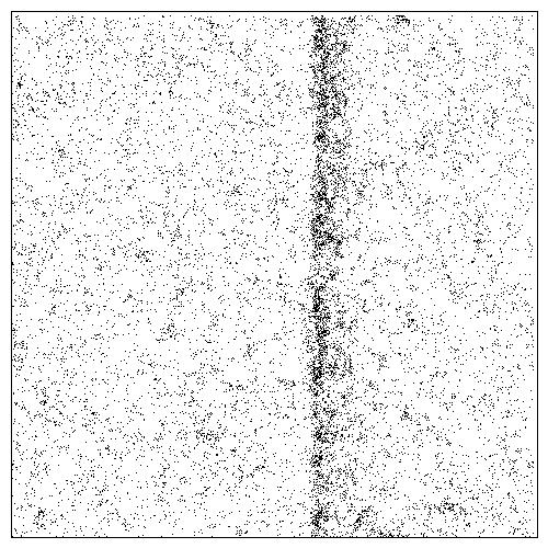
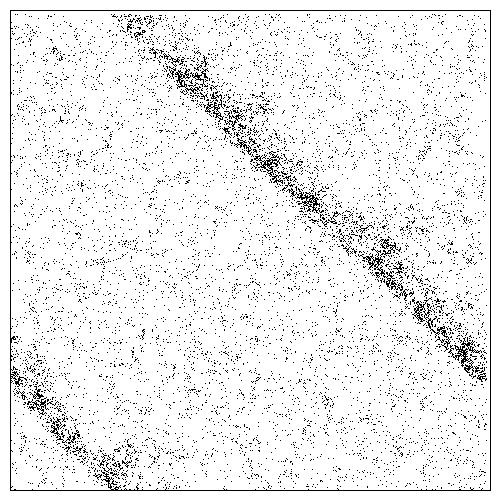
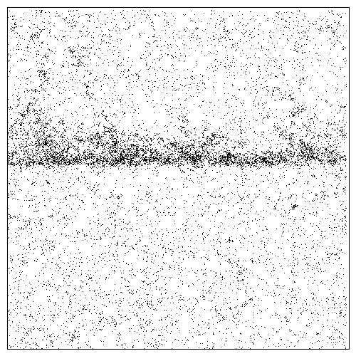
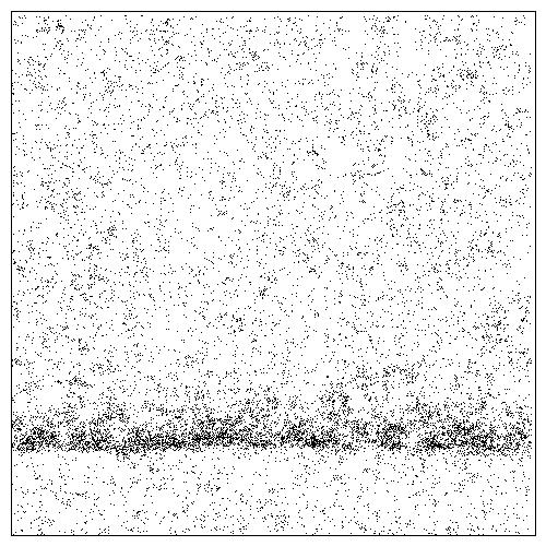
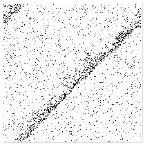
2.262	2.140	2.100	2.080	2.060
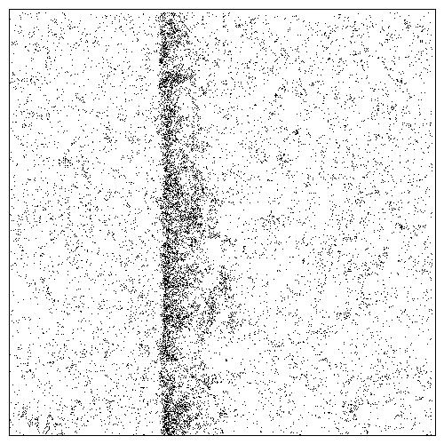
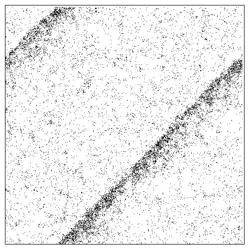
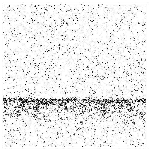
2.020	1.950	1.900	1.850	1.800
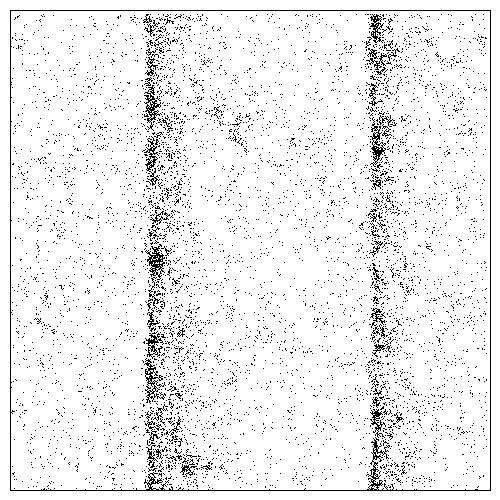
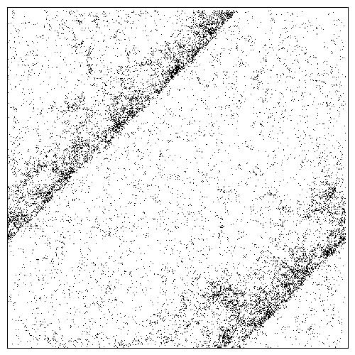
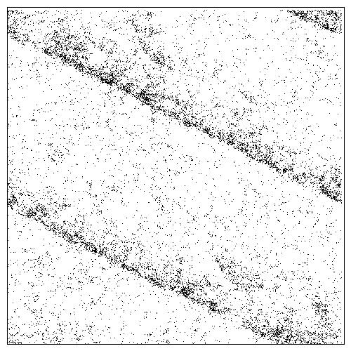
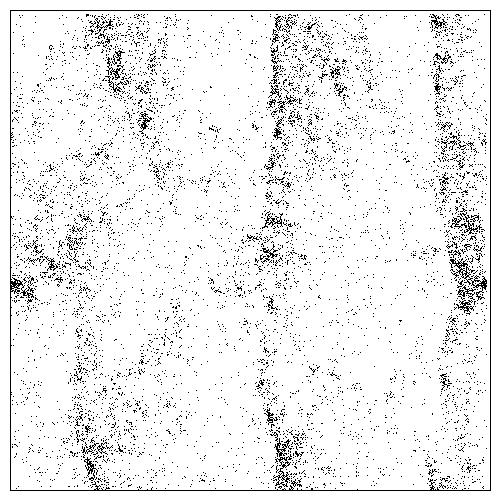
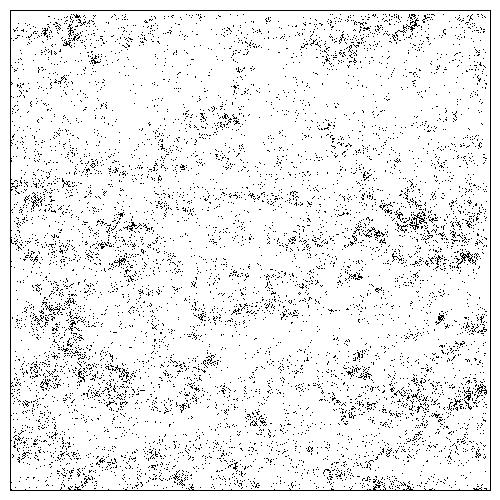
1.740	1.700	1.600	1.250	0.500

Figure 4: $L=128$: Band structures have been shown for fifteen different stationary states evolved from the same initial state but subjected to noise strength $\eta$ of different magnitudes mentioned under the figure. Brief description of the individual bands are given in Table I.

$\eta$	$\phi$	$\Omega$	Wrapping	Description
2.262	$\pi$	0.173	$W(1,0)$	Single vertical band.
2.140	$5\pi/4$	0.303	$W(1,1)$	Single diagonal band.
2.100	$3\pi/2$	0.329	$W(0,1)$	Single horizontal band.
2.080	$3\pi/2$	0.342	$W(0,1)$	Single horizontal band.
2.060	$7\pi/4$	0.382	$W(1,1)$	Single diagonal band.
2.020	$\pi$	0.379	$W(1,0)$	Single vertical band.
1.950	$3\pi/4$	0.443	$W(1,1)$	Single diagonal band.
1.900	$\pi/2$	0.450	$W(0,1)$	Single horizontal band.
1.850	$\pi/2$	0.505	$2W(0,1)$	Two parallel horizontal bands.
1.800	$7\pi/4$	0.520	$W(1,1)$	Single diagonal band.
1.740	$\pi$	0.562	$2W(1,0)$	Two vertical bands.
1.700	$7\pi/4$	0.568	$W(1,1)$	Single diagonal band.
1.600	$3\pi/2-arctan(1/2)$	0.617	$W(1,2)$	Single multiply wrapped band.
1.250		0.761		Parallel bands become blurred.
0.500		0.949		Bands are absent.

Table 1: $L$ = 128: Brief descriptions of different types of bands.

How the system becomes increasingly ordered as the strength of the applied noise is systematically reduced? To understand it we need to follow the formation of bands. When $\eta$ is tuned to $\eta_{c}(L)$ a band of agents of high density appears in the system for the first time. Within a band, the motion of the agents are directed. Such a band has the shape of a thin and straight strip which moves as a whole along a specific direction perpendicular to the length of the band. Because of the imposed periodic boundary condition, the band takes the shape of a closed ring. Consequently, the magnitude of the order parameter jumps discontinuously to a non-zero value when a band appears in the system. In general, for $\eta<\eta_{c}$ the bands can be oriented along different directions, e.g., parallel to the sides, along the diagonal directions, or even along some other directions. The shapes of the bands become increasingly non-trivial as the system size becomes larger. For such large system sizes multiple bands can also be simultaneously present.

A band consists of a set of directionally biased agents moving along almost (apart from noise) in the same direction. The entire band moves in a sea of randomly diffusing agents. Thus, the whole $L\times L$ area is divided into two zones: the band, comprised of the directed agents and the diffusive zone, comprising of the rest of the diffusive agents. At every instant the band does two activities simultaneously: (i) It absorbs fresh agents into it at its front edge picking them from the diffusive zone which execute a directed motion inside the band, and (ii) simultaneously it pushes the directed agents at the back edge of the band into the diffusive zone. The rates of these two processes are equal and in that way the width and shape of the band is maintained in the stationary state. The front edge of the band is sharp where as the back edge is hazy. Therefore, when there is only one band present in the system, an arbitrarily tagged agent has two types of motion: for a certain amount of time it executes a diffusive motion, and then it is swallowed by the band at the front edge. It then moves with the band for a little while as a directed agent, and then again dropped out in the diffusive region from the back edge. In the stationary state, this type of motion is repeated ad infinitum for all agents.

Figure 5: $L=128$: The average value of the order parameter $\Omega(\eta,L)$ in the stationary state has been plotted against the noise strength $\eta$ using black opaque circles. At the critical noise $\eta_{c}(L)=2.2645$ there is a sharp rise in the order parameter. In the sub-critical regime three distinct data sets are identified which correspond to three different shaped bands and are plotted with circles filled with different colors: $W(1,0)$ and $W(0,1)$ (blue); $2W(1,0)$ and $2W(0,1)$ (red); $W(1,1)$ (green). In each set the $\Omega(\eta,L)$ increases almost linearly on decreasing $\eta$.

In the following we report the results of our numerical study on three different system sizes, namely $L$ = 128, 256 and 512. We have observed how the discontinuous transition becomes more vivid and the band structure become increasingly rich as the system size is systematically enlarged.

III 3. Results

III.1 System size L = 128

We first exhibit the variation of the instantaneous order parameter $\Omega(t,\eta,L)$ against time $t$ in Fig. 2. Three figures corresponding to three closely separated values of the noise parameter $\eta$ = 2.262, 2.266 and 2.270 have been shown in the top, middle and bottom panels. The same random initial state has been used in all three cases. In each case, the data has been plotted at the interval of every 1000 time steps and the time series has been shown for 30 million time steps. It is apparent from the plot that the system evolves through two possible metastable states, an ordered state with high value of $\Omega$ and a disordered state with a very small value of $\Omega$. The system flip-flops between these two states. It can also be observed that the system spends more time in the ordered state with smaller noise at $\eta=2.262$. On the other hand, the typical residence time in the disordered state is longer with larger value of $\eta$ = 2.270. However, in between at $\eta$ = 2.266, the system resides in both states almost equally frequently. Therefore, we approximately estimate $\eta_{c}$ = 2.266 as the critical noise parameter of the system for $L=128$.

Figure 6: $L=256$: Plot of the instantaneous order parameter $\Omega(t,\eta,L)$ against time as in Fig. 2 for $\eta=$ 2.346, 2.348 and 2.350 (from top to bottom). Here the system is not seen to flip-flop between two metastable states. Since the system evolves from a randomly selected state, initially the system is in a disordered state without any band having a nearly vanishing value of $\Omega$ but then it suddenly jumps to an ordered state on the appearance of a correlated band.

To quantify the metastable states we have estimated the probability distribution of the order parameter $P(\Omega,\eta,L)$ (Fig. 3). It has been found that for all three noise levels, the probability distribution has double peaks at two distinct values of $\Omega$. These humps correspond to the ordered and disordered states. For small $\eta=2.2610$, the peak in the ordered state is taller than its peak in the disordered state. On the other hand, for large $\eta=2.2680$, it is the opposite, i.e., the peak in the disordered state is taller than its peak in the ordered state. For the third plot with $\eta=2.2645$ both peaks are approximately of same heights.

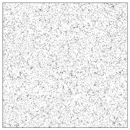
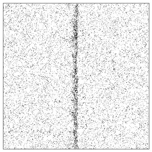
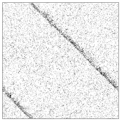
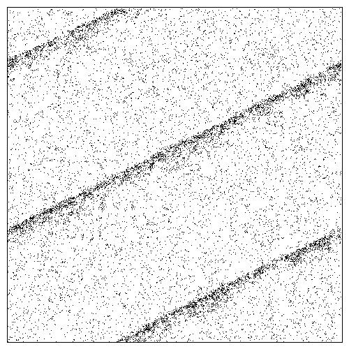
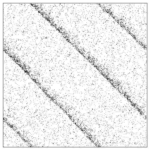
2.360	2.340	2.320	2.100	1.980
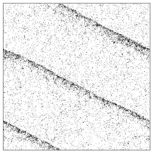
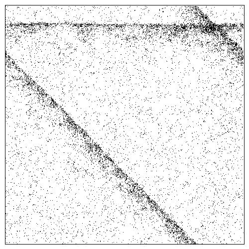
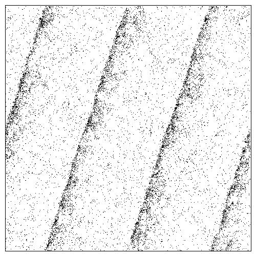
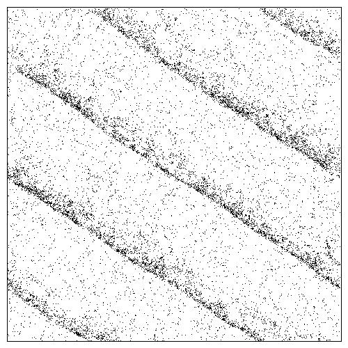
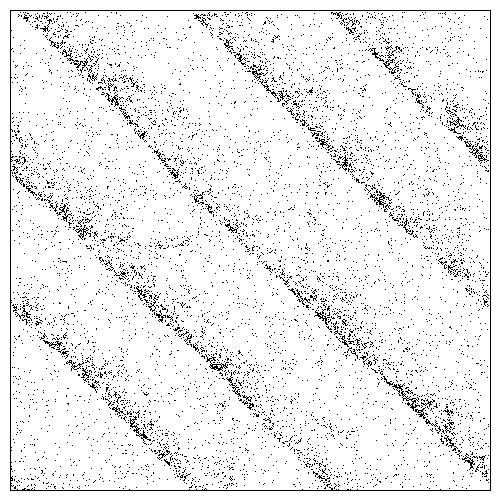
1.940	1.800	1.750	1.700	1.600
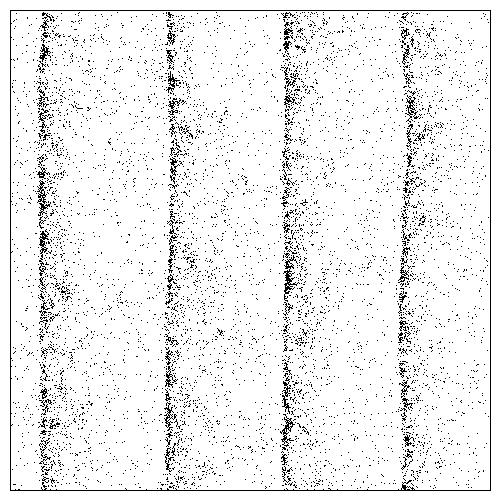
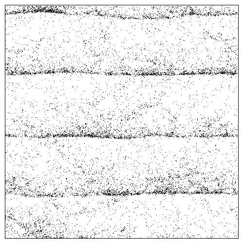
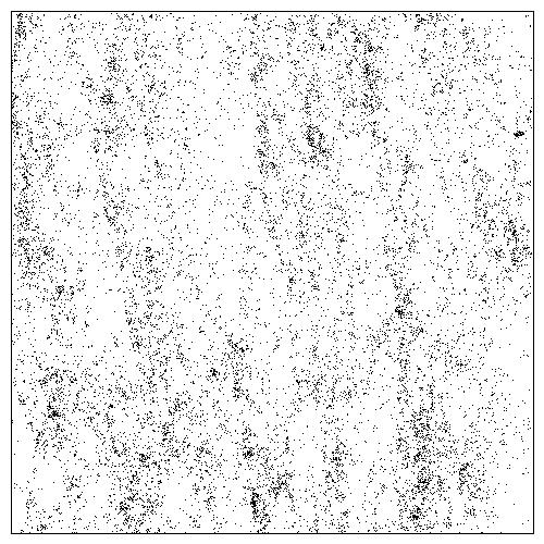
1.550	1.400	1.300	1.000	0.100

Figure 7: $L$ = 256: Band structures in fifteen different stationary states evolved from the same initial positions and velocities but subjected to noise $\eta$ of different strengths have been exhibited using 16384 randomly selected agents. The description of the individual bands are given in Table II.

$\eta$	$\phi$	$\Omega$	Wrapping	Description
2.360		0.009		Disordered state without band.
2.340	0	0.149	$W(1,0)$	Single vertical bond.
2.320	$5\pi/4$	0.189	$W(1,1)$	Single diagonal band.
2.100	$\pi/2+arctan(1/2)$	0.345	$W(1,2)$	Single multiply wrapped band.
1.980	$5\pi/4$	0.429	$2W(1,1)$	Two parallel diagonal bands.
1.940	$\pi/2-arctan(1/2)$	0.437	$W(1,2)$	Single multiply wrapped band.
1.800	$\pi/2,\pi/4$	0.488	$W(0,1)$, $W(1,1)$	Crossing: A diagonal and a horizontal band.
1.750	$\pi-arctan(3)$	0.549	$W(3,1)$	Single multiply wrapped band.
1.700	$3\pi/2-arctan(2/3)$	0.577	$W(2,3)$	Single band, wrapped four times.
1.600	$5\pi/4$	0.620	$3W(1,1)$	Three parallel diagonal bands.
1.550	$\pi$	0.647	$4W(1,0)$	Four parallel vertical bands.
1.400	$3\pi/2$	0.710	$4W(0,1)$	Four parallel horizontal bands.
1.300		0.739		Some distorted and hazy bands.
1.000		0.838		Ordered state without band.
0.100		0.997		Ordered state without band.

Table 2: $L$ = 256: Brief descriptions of different types of bands.

In Fig. 4 snapshots of fifteen agent configurations have been shown, and the characterization of each figure has been done in Table 1. Presence of bands have been searched for in the stationary states of the system. We started from a high value of $\eta$ and the reduced its value systematically in small intervals. The first high density stable band is observed for $\eta=2.262$. The flip-flop dynamics of the system exhibited in Fig. 2 implies the appearance and disappearance of such bands with time. The orientation of the band is measured by the angle $\phi$ between the direction of motion of the band and the positive $x$ direction. All bands always move along the normal to the front edge of the band. Therefore, for the first few snapshots of Fig. 4, the angle $\phi$ has the values $\pi$, $5\pi/4$, $3\pi/2$, $3\pi/2$, $7\pi/4$, … etc. The first diagonal band appeared at $\eta=2.140$. The first parallel double bands appeared at $\eta=1.850$. The next non-trivial band appeared at $\eta=1.600$ with $\phi=3\pi/2-arctan(1/2)$.

The bands are stable and with the periodic boundary condition imposed, they wrap the system different number of times in different snapshots. For example, if the orientation of the band is neither horizontal nor vertical, it must be oriented at an angle $\phi$ such that it wraps the system. We characterize such a wrapped band by an integer pair $W(m,n)$ such that the numbers of its intersection are $m$ and $n$ with the $x$ and $y$ axes respectively and $\phi$ differs from arctan($m/n$) either by $\pm\pi/2$ or by $\pm\pi$. For example, $W(1,0)$ and $W(0,1)$ are the vertical and horizontal bands respectively. A single diagonal band is denoted by $W(1,1)$. A set of $k$ parallel $W(m,n)$ bands are denoted by $kW(m,n)$.

Figure 8: $L=256$: The average value of the order parameter $\Omega(\eta,L)$ in the stationary state has been plotted against the noise strength $\eta$ using black opaque circles. At the critical noise $\eta_{c}(L)=2.350$ there is a sharp rise in the order parameter similar to a discontinuous transition. In the subcritical regime four different data sets are identified with four distinctly different shaped bands and are represented by filled circles of different colors: $W(1,1)$ (red); $2W(1,1)$ (blue); $4W(1,0)$ and $4W(0,1)$ (magenta) and $W(1,2)$ and $W(2,1)$ (green). In each set the $\Omega(\eta,L)$ increases almost linearly on decreasing $\eta$.

Therefore, it is apparent that as $\eta$ decreases the agents become more strongly correlated. Such stronger correlation appears in longer lengths as well as wider widths of the bands. Long band lengths are accommodated by increasing the number of bands, selecting the non-trivial orientation of the bands, or by increasing the wrapping numbers. When $\eta$ is tuned down to $\approx$ 1.250, the distinct structure of bands start vanishing, i.e., the dismantling process of the bands start. Evidently, no distinct band was observed when $\eta$ was set to even smaller values.

The variation of the order parameter $\Omega(\eta,L)$ for $L=128$ against the noise strength $\eta$ has been shown in Fig. 5. For $\eta<\eta_{c}(L)$ the order parameter $\Omega(\eta,L)$ increases almost linearly on reducing $\eta$. It is clear that the entire plot is the combination of different subset of points corresponding to different shaped bands. In Fig. 5 we have marked three sets of colored circles that represent the data for three types of bands. For $\eta>\eta_{c}(L)$ the $\Omega(\eta,L)$ assumes a nearly constant value close to zero on increasing $\eta$.

Figure 9: $L=512$: Variation of the instantaneous order parameter $\Omega(t,\eta,L)$ has been shown against time $t$ and for $\eta=$ 2.350, 2.360, and 2.370 (from top to bottom). As $\eta$ approaches $\eta_{c}$, increasingly longer time is required for switching over from the disordered to the ordered state.

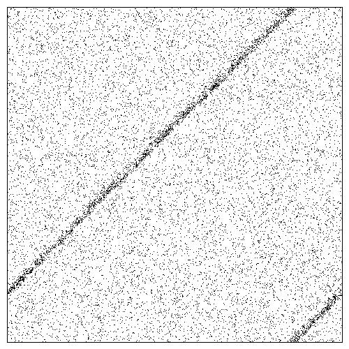
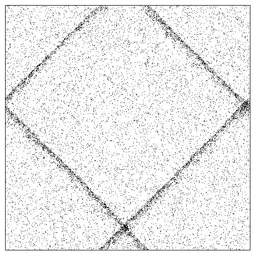
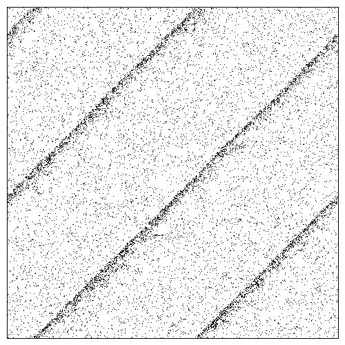
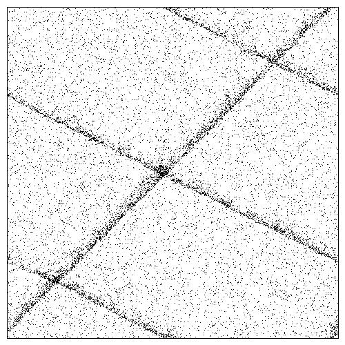
2.368	2.130	2.110	2.100	2.090
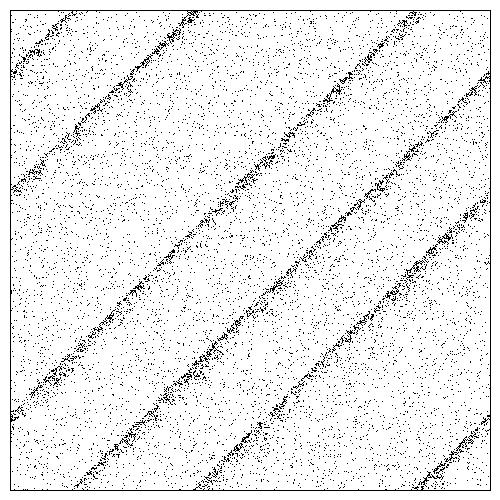
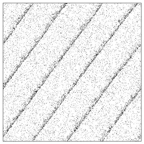
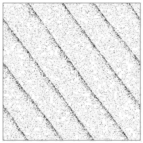
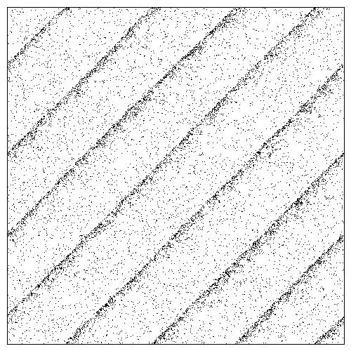
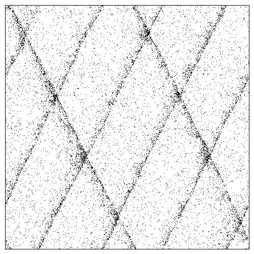
2.040	2.000	1.980	1.900	1.800
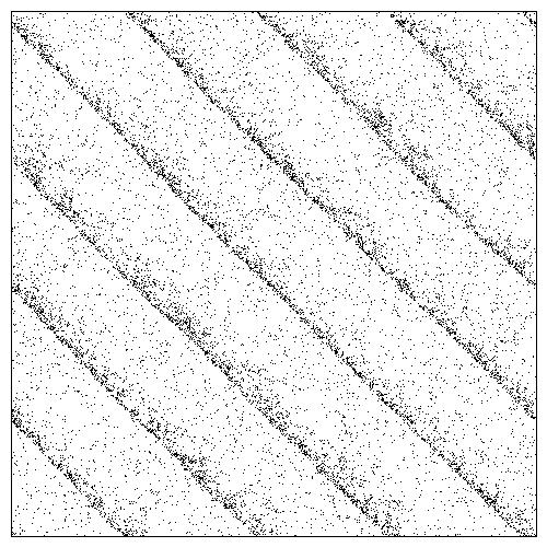
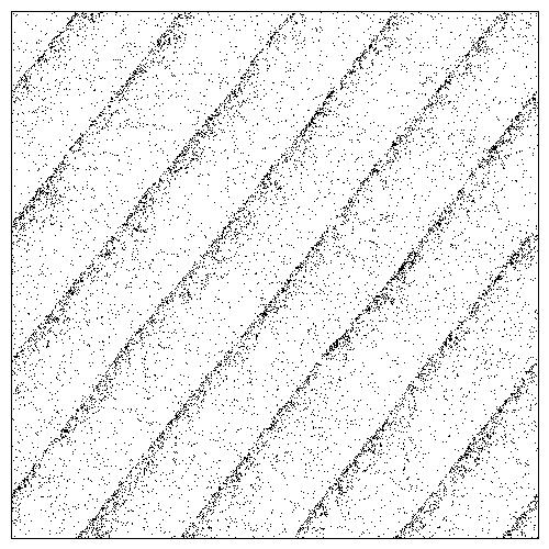
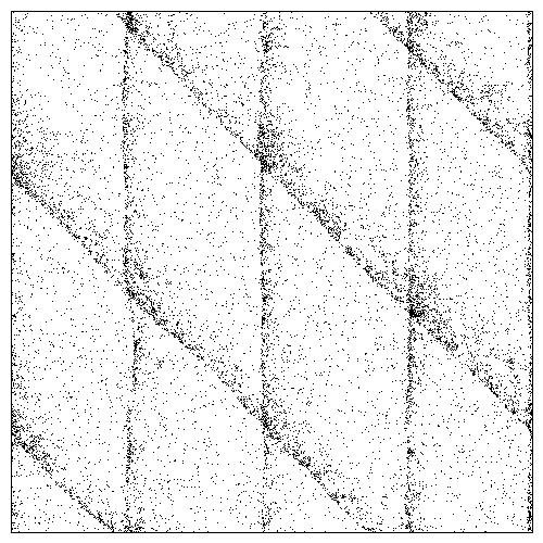
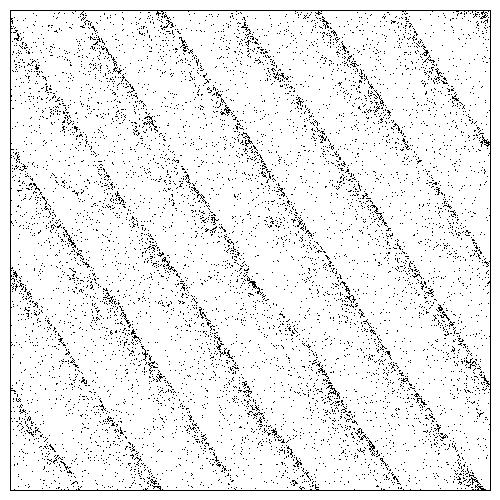
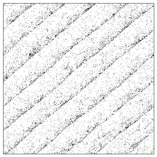
1.750	1.700	1.650	1.550	1.500
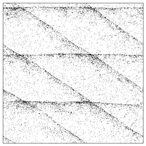
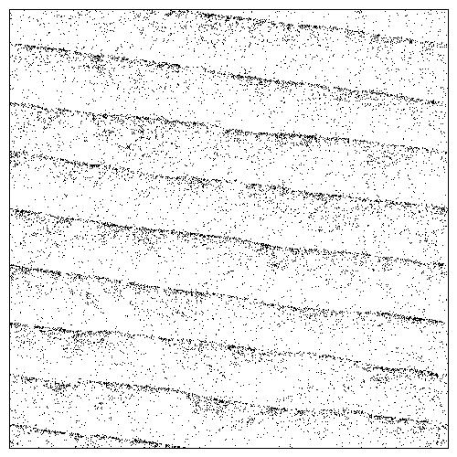
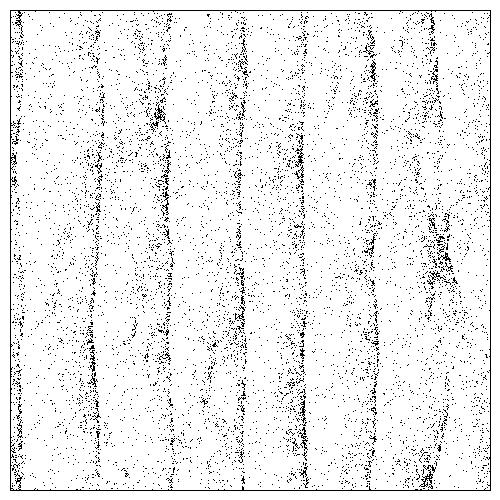
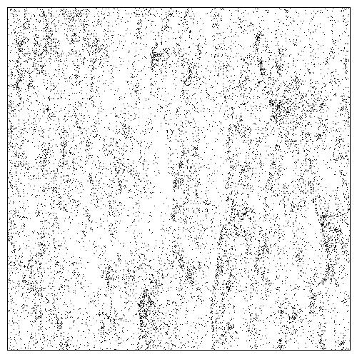
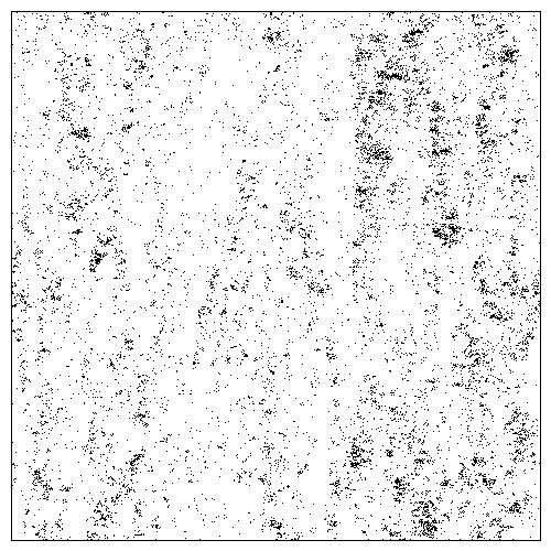
1.450	1.400	1.350	1.000	0.100

Figure 10: $L$ = 512: Band structures in twenty different stationary states evolved from the same initial positions and velocities but subjected to noise $\eta$ of different strengths have been exhibited using 16384 randomly selected agents. The description of the individual bands are given in Table III.

$\eta$	$\phi$	$\Omega$	Wrapping	Description
2.368	$7\pi/4$	0.115	W(1,1)	Single diagonal band.
2.130	$\pi/4,4\pi/4$	0.227	W(1,1),W(1,1)	Crossing of two diagonal bands at right angle.
2.110	$3\pi/4$	0.326	2W(1,1)	Two parallel diagonal bands.
2.100	$\pi/4$	0.350	3W(1,1)	Three parallel diagonal bands.
2.090	$7\pi/4,3\pi/2-arctan(1/2)$	0.288	W(1,1),W(1,2)	Crossing of two sets of bands.
2.040	$3\pi/4$	0.384	3W(1,1)	Three parallel diagonal bands.
2.000	$3\pi/2+arctan(4/3)$	0.413	W(4,3)	A single band that wraps multiple times.
1.980	$\pi/2-arctan(4/3)$	0.424	W(4,3)	A single band that wraps multiple times.
1.900	$3\pi/4$	0.472	4W(1,1)	Four parallel diagonal bands.
1.800	$\pi/2-arctan(2),3\pi/2+arctan(2)$	0.489	W(2,1) and 2W(2,1)	Crossing of two sets of bands.
1.750	$5\pi/4$	0.546	4W(1,1)	Four parallel diagonal bands.
1.700	$\pi-arctan(5/4)$	0.574	W(5,4)	A single band that wraps multiple times.
1.650	$\pi,5\pi/4$	0.570	4W(1,0),2W(1,1)	Crossing of two sets of bands.
1.550	$\pi/2-arctan(6/4)$	0.642	2W(3,2)	Two parallel multiply wrapped bands.
1.500	$3\pi/2+arctan(5/6)$	0.663	W(5,6)	A single band that wraps multiple times.
1.450	$\pi/2,\pi/2-arctan(3/2)$	0.670	3W(0,1),W(2,3)	Crossing of two sets of bands.
1.400	$\pi/2-arctan(1/8)$	0.709	W(1,8)	Single multiply wrapped band.
1.350		0.724	7W(1,0)	Seven parallel vertical bands.
1.000		0.838		No band structure is found.
0.100		0.996		No band structure is found.

Table 3: $L$ = 512: Brief description of different types of bands.

Figure 11: $L$ = 512: The stationary state order parameter $\Omega(\eta,L)$ has been plotted against the noise strength $\eta$. The critical value $\eta_{c}(L)$ of transition has been found to 2.368. In the sub-critical regime six distinct sub-sets of data points have been identified for six differently shaped bands. They are grouped together and labeled by their wrapping numbers: $W(1,1)$ (red); $2W(1,1)$ (brown); $3W(1,1)$ (blue); $4W(1,1)$ (magenta); $W(4,3),W(3,4)$ (green) and $W(1,1),W(1,1)$ bands are presented by maroon color.

III.2 System size L = 256

Here also the dynamics starts from the same completely random initial state for all values of the noise strength parameter $\eta$, and therefore the motion of the agents are predominantly diffusive at the early stage. As time is elapsed, the system takes time to organize itself. Typically, after a substantial amount of relaxation time, bands are formed here as well. In contrast to the situation in $L=128$ system, here the system does not flip-flop between two metastable states. Consequently, the magnitude of the order parameter jumps up only for once from a nearly vanishing value to a finite magnitude. Three such jumps have been shown in Fig. 6 where the time series for the order parameter has been plotted against time for the 20 million time steps. For the noise level of $\eta$ = 2.346, 2.348, and 2.350 the transitions take place at times $\approx$ 18, 9 and 5 million respectively.

Similar to the previous case, fifteen snapshots of the agent configurations have been shown in Fig. 7 for $L=256$. These snapshots are taken at long times after the jumps to the ordered states have taken place. Here a number of bands of different orientations and wrappings have been observed. Compared to $L=128$ we find here a new type of stationary state where two different sets of bands cross one another. For example, in case of $\eta=1.800$, we have exhibited a snapshot where a single horizontal band $W(0,1)$ with $\phi=\pi/2$ crosses a single diagonal band $W(1,1)$ with $\phi=\pi/4$. Both bands are stable and move along two different directions, separated by $\pi/4$. In general, for such crossed bands, the order parameter takes slightly smaller values.

In Fig. 8 the time averaged value of the order parameter $\Omega(\eta,L)$ has been plotted against $\eta$. The sharp fall in the order parameter takes place at $\eta_{c}(L)\approx 2.350$. Beyond this value of $\eta>\eta_{c}(L)$, order parameter is nearly zero. For $\eta<\eta_{c}(L)$ four sets of data points are plotted which correspond to four different band structures as explained in the figure caption.

III.3 System size L = 512

The bands become most clearly visible for the system size $L=512$. Because of the choice of random orientation angles of the velocity vectors, the initial state is disordered with vanishingly small value of the order parameter. Beyond the critical noise value $\eta_{c}=2.368$ the order parameter in the stationary state assumes a very small value. However, when the noise is reduced, $\Omega(\eta_{c},L)$ jumps discontinuously at $\eta_{c}$ to a finite value. In Fig. 9 the instantaneous value of the order parameter $\Omega(t,\eta,L)$ has been plotted against time for long durations. For $\eta$ = 2.350 and 2.360 discontinuous jumps to the ordered state are observed after approximately 9 and 21 million time steps. In the bottom curve, $\eta=2.370$ has been used and no such jump has been observed within the entire duration of observation of 35 million time steps.

Therefore in general, the long time stationary states of all states for $\eta<\eta_{c}(L)=2.368$ have been observed to be characterized by the presence of bands of high density directed agents. As the value of the noise strength $\eta$ is systematically decreased different types of bands appear in the stationary states. In Fig. 10 we have exhibited twenty snapshots of agent locations in these stationary states of $L$ = 512. We have observed single and multiple bands, diagonal and non-diagonally oriented bands, crossed bands meeting perpendicular to one another or at an angle, and also bands which wrap the system multiple times. For $0<\eta<1$ the clearly visible band structure has been missing till our time of observation of 50 million time steps. In Table III we describe the band structures of these twenty stationary states. The value of $\eta$ has been mentioned below every plot.

In Fig. 11 we have plotted $\Omega(\eta,L)$ against $\eta$. Here also, in the ordered state the points for different types of bands form different groups. Within one group the band pattern is the same for all values of $\eta$ but the value of $\Omega(\eta,L)$ increases linearly on decreasing $\eta$. Six such group of points have been shown in Fig. 11 and the corresponding wrapping numbers have been mentioned in the caption.

Before we summarize we like to emphasize two points. First, we try to visualize the motion of crossed bands where the direction of motion of each band is perpendicular to its sharp edge. As the system evolves the bands move through each other, but because of the periodic boundary condition, they always remain entangled and cannot be detached from each other. In principle, the simultaneous appearance of three or more different sets of bands crossed among themselves may be quite possible, may be for larger system sizes, but we have not observed them. In Fig. 12 we present four snapshots of the crossed bands at a small interval of 100 time units to exhibit their motion. Two parallel $W(1,0)$ bands are crossed by one $W(1,1)$ band and all three bands move perpendicular to their front edges.

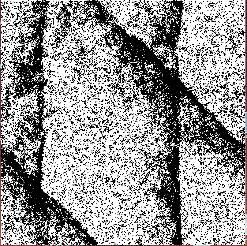
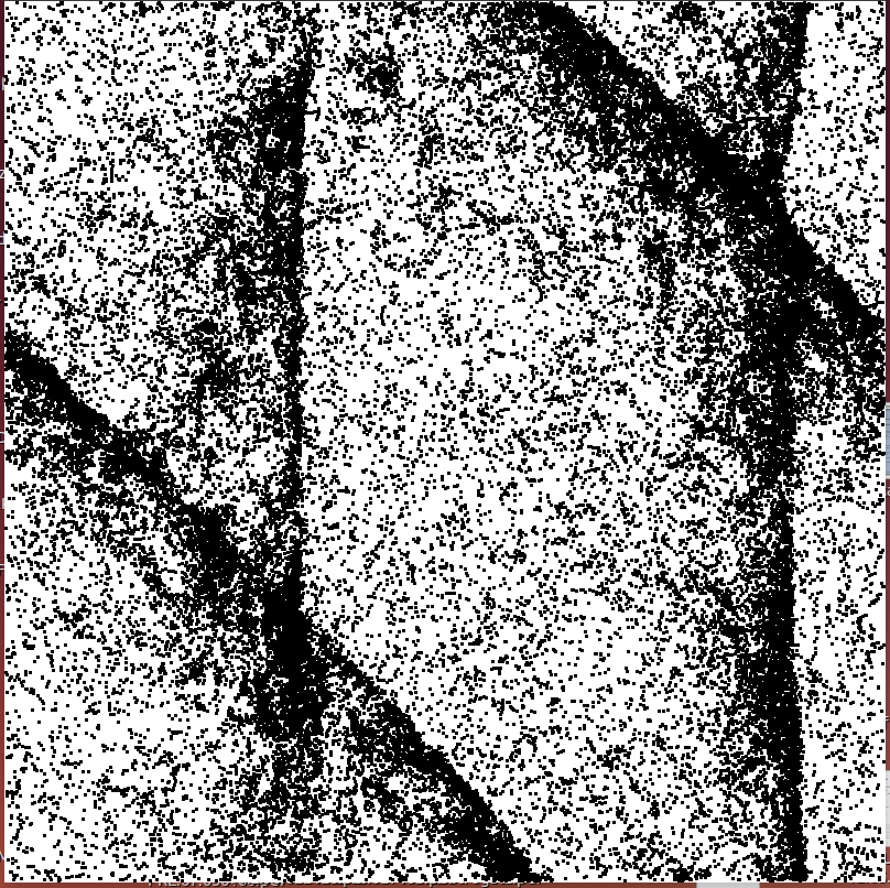
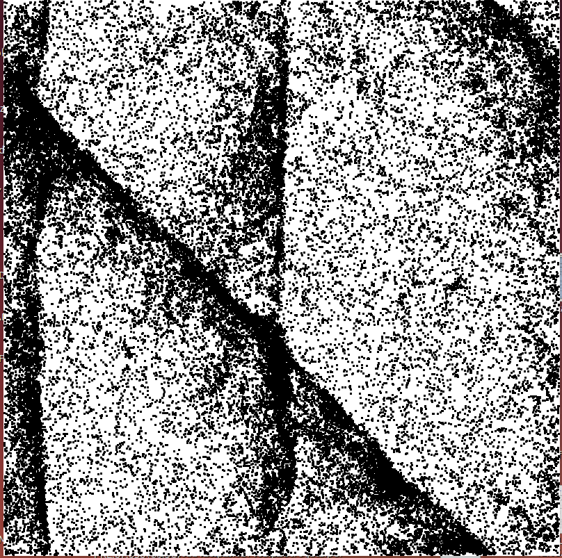
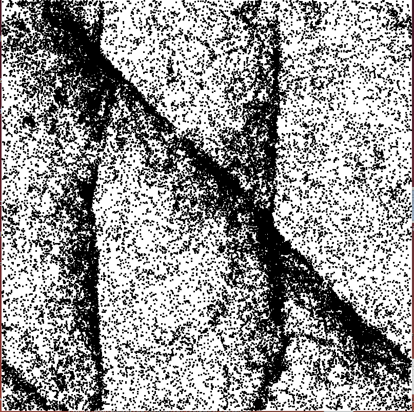
Figure 12: Crossed band configurations at the stationary state for a system size $L$ = 256, $\eta$ = 1.8, and with density $\rho=1$ of the agents. Starting from an arbitrary initial configuration, the system arrives at the stationary having two W(1,0) bands and one W(1,1) band. Four snapshots have been shown at the interval of 100 time steps from left to right. These figures exhibits that W(1,0) bands are moving to the right and the W(1,1) bond is moving towards the top-right direction.

Secondly, in Fig. 13 we present four snapshots of the stationary state bands starting from four different initial configurations of positions and velocities of the agents, the strength $\eta$ of the noise being maintained the same. We have obtained different wrapping patterns in each case. It may be quite possible that there are more patterns, and starting from a random initial configuration the system may evolve to any one of the band patterns in the stationary state. We also believe that the probabilities of occurrence of these steady states are likely to be distinct and possibly function of $\eta$. However, to estimate this probability distribution numerically needs high value of computational resources and unfortunately we could not afford that. Figs. 4, 7 and 10 have different system sizes, namely $L$ = 128, 256, and 512. We observed that larger the system size, more and more complicated bands with larger values of $m$ and $n$ appear in the stationary states.

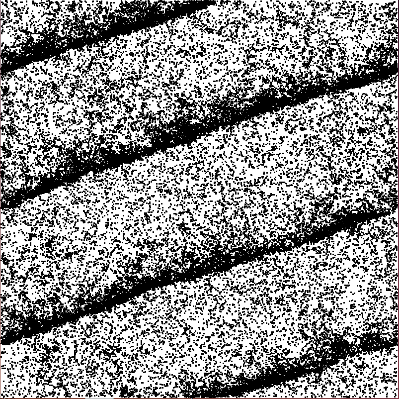
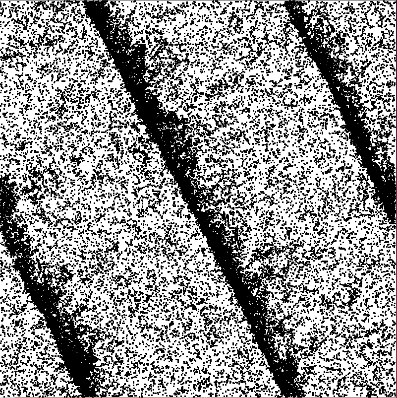
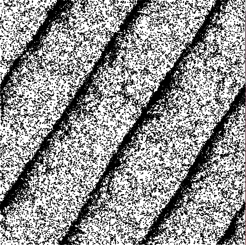
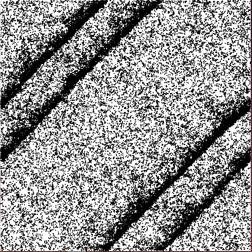
Figure 13: Different band configurations at the stationary state for a system size $L$ = 256, $\eta$ = 2.2, and with density $\rho=1$ of the agents. Different sets of initial positions of the agents and different directions for their initial velocities have been used to simulate these systems. The stationary state band configurations are quite different e.g., starting from the left we get $W(1,3)$, $W(2,1)$, $W(3,2)$, and $2W(1,1)$ bands.

IV 4. Summary

To summarize, we have studied the Vicsek model of collective motion with quenched range of interaction. For studying the two dimensional version of the model with scalar noise, the underlying plane has been divided into non-overlapping square shaped neighborhoods. All agents residing within a certain square cell at a certain time are mutual neighbors of one another. Direction of the resultant of their velocity vectors is assigned to all agents which are then topped up by applying random noise. In a microscopic description of the model it has been argued that the agents in two adjacent cells having similar velocity directions feel certain cohesiveness and therefore continue their motion in the adjacent cells. This cohesiveness property of moving together along the same direction is the original cause for the formation of band structures in the models of collective motion in the framework of the Vicsek model. Within a band, the agents are correlated. As the noise decreases the sub-critical regime, the correlation becomes stronger. Consequently the system becomes more ordered which is reflected in the non-trivial shaped bands of longer lengths, larger widths, different orientations and wrapping numbers. We have formulated a detailed prescription for the characterization of such bands. Starting from the completely disordered regime, as the strength of the noise is tuned down systematically, the most simple band parallel to the edges pops up abruptly, indicating a discontinuous transition similar to the Vicsek model.

By introducing the quenched range of interaction we have reduced, the individual freedom of the agents. In a way, this can be looked upon as feeding more correlation among the agents. It seems likely, that because of this extra correlation many different shaped bands show up in our model, even for the system size $L=512$. Appearance of similar bands may be plausible even in the original Vicsek model for the larger system sizes and with smaller noise.

We thank the referee for pointing out that wrapping patterns of occupied sites are observed in the model of percolation as well Pinson . In a similar way a pair of numbers $(m,n)$ have been used to characterize the patterns there as well.

References

- (1) T. Vicsek and A. Zafeiris, Physics Reports, 517, 71 (2012).
- (2) J. Toner, Y. Tu and S. Ramaswamy, Ann. Phys. 318, 170 (2005).
- (3) J. Toner and Y. Tu, Phys. Rev. Lett. 75, 4326 (1995).
- (4) D. L. Blair and A. Kudrolli, Phys. Rev. E 67, 041301 (2003).
- (5) A. Czirok, H. E. Stanley, and T. Vicsek, J. Phys. A 30, 1375 (1997).
- (6) P. Szabó, M.Nagy and T. Vicsek, Phys. Rev. E 79, 021908 (2009).
- (7) E. Ben-Jacob, I. Cohen, O. Shochet, A. Czirók and T. Vicsek, Phys. Rev. Lett. 75, 2899 (1995).
- (8) E. Rauch, M. Millonas and D. Chialvo, Phys. Lett. A 207, 185 (1995).
- (9) C. Feare, The Starling (Oxford: Oxford University Press) (1984).
- (10) S. Hubbard, P. Babak, S. Sigurdsson and K. Magnusson, Ecol. Model. 174, 359 (2004).
- (11) T. Vicsek, A. Czirók, E. Ben-Jacob, I. Cohen, and O. Shochet, Phys. Rev. Lett., 75, 1226 (1995).
- (12) M. Aldana, V. Dossetti, C. Huepe, V. M. Kenkre, and H. Larralde, Phys. Rev. Lett. 98, 095702 (2007).
- (13) H. Chaté, F. Ginelli, and R. Montagne, Phys. Rev. Lett. 96, 180602 (2006).
- (14) A. Baskaran and M. C. Marchetti, Phys. Rev. Lett. 101, 268101 (2008).
- (15) S. Mishra, K. Tunstrom, I. D. Couzin, and C. Heupe, Phys. Rev. E 86, 011901 (2012).
- (16) H. Chaté, F. Ginelli, Guillaume Grégoire, and F. Raynaud, Phys. Rev. E 77, 046113 (2008).
- (17) B. Bhattacherjee, S. Mishra, and S. S. Manna, Phys. Rev. E, 92, 062134 (2015).
- (18) M. Ballerini et. al., Proc. Natl. Acad. Sci. 105, 1232-1237 (2008).
- (19) E. Bertin, M. Droz and G. Gŕegoire, Phys. Rev. E 74, 022101 (2006).
- (20) H. Chaté, F. Ginelli, Guillaume Grégoire, and F. Raynaud, Phys. Rev. E 77, 046113 (2008).
- (21) H. Chaté, F. Ginelli and R. Montagne, Phys. Rev. Lett., 96, 180602-180605 (2006).
- (22) F. Ginelli, F. Peruani, M. Bär and H. Chaté, Phys. Rev. Lett., 104, 184502 (2010).
- (23) H. Chaté, F. Ginelli, G. Grégoire, F. Peruani and F. Raynaud Eur. Phys. J. B, 64, 451-456 (2008).
- (24) H. T. Pinson, J. Stat. Phys. 75, 1167 (1994).