Sorkin-Johnston vacuum for a massive scalar field in the 2D causal diamond

Abstract

We study the massive scalar field Sorkin-Johnston (SJ) Wightman function $W_{SJ}$ restricted to a flat 2D causal diamond $\mathcal{D}$ of linear dimension $L$. Our approach is two-pronged. In the first, we solve the central SJ eigenvalue problem explicitly in the small mass regime, up to order $(mL)^{4}$. This allows us to formally construct $W_{SJ}$ up to this order. Using a combination of analytical and numerical methods, we obtain expressions for $W_{SJ}$ both in the center and the corner of $\mathcal{D}$, to leading order. We find that in the center, $W_{SJ}$ is more like the massless Minkowski Wightman function $W^{\mathrm{mink}}_{0}$ than the massive one $W^{\mathrm{mink}}_{m}$, while in the corner it corresponds to that of the massive mirror $W^{\mathrm{mirror}}_{m}$. In the second part, in order to explore larger masses, we perform numerical simulations using a causal set approximated by a flat 2D causal diamond. We find that in the center of the diamond the causal set SJ Wightman function $W^{c}_{SJ}$ resembles $W^{\mathrm{mink}}_{0}$ for small masses, as in the continuum, but beyond a critical value $m_{c}$ it resembles $W^{\mathrm{mink}}_{m}$, as expected. Our calculations suggest that unlike $W^{\mathrm{mink}}_{m}$, $W_{SJ}$ has a well-defined massless limit, which mimics the behavior of the Pauli Jordan function underlying the SJ construction. In the corner of the diamond, moreover, $W^{c}_{SJ}$ agrees with $W^{\mathrm{mirror}}_{m}$ for all masses, and not, as might be expected, with the Rindler vacuum.

1 Introduction

The standard approach to quantum field theory is inherently observer dependent, as is evident from the Unruh effect for accelerating observers in Minkowski spacetime. In Minkowski spacetime, due to its high degree of symmetry, there is a preferred family of inertial observers and hence a unique Poincare invariant vacuum. This Minkowski vacuum is considered the bedrock of quantum field theory, and its Poincare invariance can be used to explain many aspects of the theory.

However, in a generic curved spacetime no such preferred family of observers exists which can be used to single out a preferred vacuum state. This suggests that the state plays a subsidiary role in the theory. This is the approach taken in algebraic quantum field theory, where a primary role is played by the algebra of operators. The choice of state is relegated to a choice of representation of this algebra, which need not be coordinate invariant. A proposal for a unique vacuum state, the SJ vacuum, for a free scalar field theory was developed by Sorkin and Johnston [1, 2] for a bounded, globally hyperbolic region $M$ of a spacetime. The Pauli-Jordan integral operator, defined as

$$i\hat{\Delta}\circ f(X)\equiv\int_{M}i\Delta(X,X^{\prime})f(X^{\prime})\,dV_{X^{\prime}}$$ (1)

is self adjoint in $M$. Here, $\Delta(X,X^{\prime})$, is the covariantly defined Pauli-Jordan function (which is the difference in the retarded and advanced Green functions) and $dV_{X}$ is the volume element. The associated SJ Wightman function $W_{SJ}$ (or two point function) is then simply the positive part of $i\hat{\Delta}$. $W_{SJ}$ can be shown to be the unique vacuum which satisfies the following conditions [1, 3]

$$W(X,X^{\prime})-W(X^{\prime},X) = i\Delta(X,X^{\prime})\quad\mathrm{Commutator\;condition}$$

$$W(X,X^{\prime})-W^{*}(X^{\prime},X) = 0\quad\mathrm{Hermiticity}$$

$$\int_{M}dV_{X}\,dV_{Y}\,f^{*}(X)W(X,Y)f(Y) \geq 0\quad\mathrm{Positive\;semidefinite}$$

$$\int_{M}dV_{X^{\prime}}\,W(X,X^{\prime})W(X^{\prime\prime},X^{\prime}) = 0\quad\mathrm{orthogonal\;support}.$$ (2)

$W_{SJ}$ can be explicitly constructed from the spectral decomposition of $i\hat{\Delta}$, where the spectrum of $i\hat{\Delta}$ is given by the integral eigenvalue equation

$$i\hat{\Delta}\circ u(X)=\lambda\,u(X).$$ (3)

This is what we refer to as the “central eigenvalue problem” in the SJ approach.

However the integral form makes it a challenging task to find solutions even in simple cases. As a result there are very few cases in which $W_{SJ}$ has been obtained explicitly. These include the massless free scalar SJ vacuum in a 2D flat causal diamond [3, 4], a patch of trousers spacetime [5] and the ultrastatic slab spacetime [6]. In this work, we study the SJ vacuum for a massive free scalar field in the 2D flat causal diamond $\mathcal{D}$ of length $2L$, both in the continuum and on a causal set ${\cal C}_{\mathcal{D}}$ obtained from sprinkling into $\mathcal{D}$.

In the continuum we solve the central SJ eigenvalue problem explicitly in the small mass approximation keeping terms only up to $\mathcal{O}(m^{4})$, with $m^{4}\ll 1$ (in dimensionless units, with $L=1$). The eigenfunctions and eigenvalues so obtained reduce to their massless counterparts when $m=0$ [3]. This allows us to formally construct $W_{SJ}$ in $\mathcal{D}$.

As in [3] we consider two regimes of interest: one in the center of the diamond, and the other at the corner. In a small central region $\mathcal{D}_{l}$ of size $l$, we find analytically that $W_{SJ}$ resembles the massless Minkowski vacuum $W^{\mathrm{mink}}_{0}$ up to a small mass-dependent constant $\epsilon_{m}^{center}$, rather than the massive Minkowski vacuum $W^{\mathrm{mink}}_{m}$. In the corner, $W_{SJ}$ resembles the massive mirror vacuum $W^{\mathrm{mirror}}_{m}$, with the difference depending on a small mass-dependent constant $\epsilon_{m}^{corner}$, rather than the expected agreement with the massive Rindler vacuum $W^{\mathrm{rind}}_{m}$. Both $\epsilon_{m}^{center}$ and $\epsilon_{m}^{corner}$ are the errors that arise in the approximation of a quantization condition which is a mass dependent transcendental equation, and are therefore non-trivial to calculate analytically.

In order to find $\epsilon_{m}^{center},\epsilon_{m}^{corner}$, we evaluate $W_{SJ}$ numerically using a convergent truncation $W_{SJ}^{t}$ of the mode-sum. The calculations show that $\epsilon_{m}^{center},\epsilon_{m}^{corner}$ contribute negligibly to $W_{SJ}$ both in the center and the corner. This confirms that for small mass $W_{SJ}$ corresponds to the massless Minkowski vacuum. This behavior is unexpected, and suggests that at least in this small mass approximation $W_{SJ}$ does not satisfy the expected massive Poincare invariance of the vacuum but rather the massless Poincare invariance. In the corner, again $\epsilon_{m}^{corner}$ is found to be small, and confirms that $W_{SJ}$ resembles $W^{\mathrm{mirror}}_{m}$ rather than $W^{\mathrm{rind}}_{m}$.

We then examine the behavior of this truncated $W_{SJ}^{t}$ in a slightly enlarged region in the center. We find that it continues to differ from $W^{\mathrm{mink}}_{m}$, while agreeing with $W^{\mathrm{mink}}_{0}$ at least up to $l\sim 0.1$. In an enlarged corner region $W_{SJ}$ there is a marked deviation from $W^{\mathrm{mirror}}_{m}$, but it still does not resemble the Rindler vacuum.

In the next part of this work we obtain $W^{c}_{SJ}$ numerically for a causal set ${\cal C}_{\mathcal{D}}$ obtained by sprinkling into $\mathcal{D}$, for a range of masses. We find that in the small mass regime $W^{c}_{SJ}$ agrees with our analytic calculation of $W_{SJ}$ in the center of the diamond and therefore resembles $W^{\mathrm{mink}}_{0}$. This means that it differs from $W^{\mathrm{mink}}_{m}$ in the small mass regime. However, as the mass is increased, there is a cross-over point at which the massless and massive Minkowski vacuum coincide. This occurs when the mass $m_{c}\equiv 2\Lambda\sim 0.924$, where $\Lambda\sim 0.462$ is the IR cut-off for the massless vacuum calculated in [3]. For $m\geq m_{c}$, $W^{c}_{SJ}$ then tracks the massive Minkowski vacuum instead of the massless Minkowski vacuum. In the corner of the diamond, the causal set $W^{c}_{SJ}$ looks like the mirror vacuum and not the Rindler vacuum for all masses.

Our calculations suggest that, as in the case of the de Sitter SJ vacuum studied in [7], the massive $W_{SJ}$ has a well defined $m\rightarrow 0$ limit, unlike $W^{\mathrm{mink}}_{m}$. A possible reason for this is that the SJ vacuum is built from the Green function which is a continuous function of $m$ even as $m\rightarrow 0$. The behavior of $W_{SJ}$ for $m>0$ is also curious. For $W^{\mathrm{mink}}_{0}$, $\Lambda$ sets a scale and dominates in the small $m$ regime, while for large $m$, the opposite is true. At $m_{c}$, $W^{\mathrm{mink}}_{0}$ and $W^{\mathrm{mink}}_{m}$ coincide at small distance scales, so that $W_{SJ}$ tracks $W^{\mathrm{mink}}_{0}$ for $m<m_{c}$ and $W^{\mathrm{mink}}_{m}$ for $m>m_{c}$ in a continuous fashion.

Whether this unexpected small mass behavior of $W_{SJ}$ is the result of finiteness of $\mathcal{D}$ or an intrinsic feature of the 2D SJ vacuum is unclear at the moment. Further examination of the massive SJ vacuum in different spacetimes should shed light on these questions. The mass dependent behavior in the 2D causal diamond echoes that in 4d de Sitter spacetime [7]. For de Sitter spacetime it is known that there is no massless de Sitter invariant vacuum, and that the Mottola-Allen vacua do not have an $m\rightarrow 0$ limit. However, for a causal set that is approximated by de Sitter spacetime $W_{SJ}^{c}$ seems to behave very differently, and in particular, does have a well defined $m\rightarrow 0$ limit. Understanding how these differences in behavior between the SJ and the standard vacua manifest themselves in the conditions Eqn (2) should shed some light. However this is beyond the scope of the present work.

We begin in Sec. 2 with a short introduction to the SJ approach to quantum field theory for free scalar field in a bounded globally hyperbolic spacetime. In Sec. 3 we set up the SJ eigenvalue problem for the massive scalar field in $\mathcal{D}$ and find the SJ spectrum in the small mass limit to $\mathcal{O}(m^{4})$. Sec. 4 contains the analytic and numerical calculations of $W_{SJ}$ in different regions of $\mathcal{D}$. In Sec. 5 we show the results of simulations of the causal set SJ vacuum $W^{c}_{SJ}$ for a range of masses. We then compare $W^{c}_{SJ}$ with the analytical calculation $W_{SJ}$ in the small mass regime, as well as with the standard vacua in the large mass regime, both in the center and the corner of the diamond for small and large values of $m$. We end with a brief discussion of our results in Section 6. Appendixes A, B and C contain the details of many of the calculations. In Appendix D we present a trick to get the 2D Rindler vacuum from the SJ prescription.

2 The SJ prescription

For a free scalar field $\hat{\phi}$, with Gaussian vacuum state $|0\rangle$, the two point function

$$W(X,X^{\prime})\equiv\left<0\left|\hat{\phi}(X)\hat{\phi}(X^{\prime})\right|0\right>$$ (4)

contains all the information about the theory. In the standard route to quantization $|0\rangle$ is itself defined using an observer dependent mode decomposition of $\hat{\phi}(x)$. The absence of a preferred class of observers for a general curved spacetime $(M,g)$ means that this mode decomposition does not lead to a preferred choice of $|0\rangle$ and thence $W(X,X^{\prime})$.

The SJ prescription provides an observer independent mode decomposition $\hat{\phi}$ defined in a compact globally hyperbolic spacetime region [1, 2, 3, 5, 6, 8, 9, 10]. Instead of an equal time commutation relation, it uses the covariant Peierls bracket

$$\left[\hat{\phi}(X),\hat{\phi}(X^{\prime})\right]=i\Delta(X,X^{\prime}),$$ (5)

where the Pauli Jordan function is given by

$$i\Delta(X,X^{\prime})=i\left(G_{R}(X,X^{\prime})-G_{A}(X,X^{\prime})\right)$$ (6)

and $G_{R}(X,X^{\prime}),G_{A}(X,X^{\prime})$ are the retarded and advanced Green functions respectively. $i\Delta(X,X^{\prime})$ is therefore imaginary and antisymmetric.

The Pauli-Jordan operator is an integral operator, Eqn (1) on the space $\mathcal{F}(M,g)$ of bounded functions in $(M,g)$ (see [11]), whose $\mathcal{L}^{2}$ inner product is

$$\left(f,g\right)\equiv\int_{M}dV_{X}f^{*}(X)g(X).$$ (7)

$i\hat{\Delta}$ is therefore self adjoint on $\mathcal{F}(M,g)$. The eigenvalues of $i\hat{\Delta}$ are therefore real and come in positive and negative pairs

$$i\hat{\Delta}\circ u_{k}=\lambda_{k}u_{k}$$

$$i\hat{\Delta}\circ u_{k}^{*}=-\lambda_{k}u_{k}^{*},$$ (8)

where $u_{k}\in\mathrm{Image}(i\hat{\Delta})$. The normalized modes $u_{k}^{SJ}=\sqrt{\lambda_{k}}u_{k}$ are referred to as the SJ modes. Since the $\{u_{k}\}$ are a complete orthonormal basis in $\mathrm{Image}(i\hat{\Delta})$, they give the following spectral decomposition

$$i\Delta(X,X^{\prime})=\sum_{k}\lambda_{k}\left(u_{k}(X)u_{k}^{*}(X^{\prime})-u_{k}^{*}(X)u_{k}(X^{\prime})\right).$$ (9)

It can be shown that [6, 11, 12]

$$\mathrm{Image}(i\hat{\Delta})=\ker(\nabla_{\mu}\nabla^{\mu}-m^{2}).$$ (10)

Thus the SJ modes are also solutions of the KG equation.

The SJ proposal is to obtain $W_{SJ}$ from $i\Delta$, without reference to preferred observers. Using the properties of $W_{SJ}$ given in Eqn. (2), it follows that

$$W_{SJ}=\mathrm{Pos}(i\hat{\Delta})\Longleftrightarrow W_{SJ}=\frac{1}{2}\left(i\hat{\Delta}+\sqrt{-\hat{\Delta}^{2}}\right)\Longleftrightarrow W_{SJ}(X,X^{\prime})=\sum_{k}\lambda_{k}u_{k}(X)u_{k}^{*}(X^{\prime}).$$ (11)

The SJ mode expansion of $\hat{\phi}(X)$ is then

$$\hat{\phi}(X)=\sum_{k}\sqrt{\lambda_{k}}\left(\hat{a}_{k}u_{k}(X)+\hat{a}_{k}^{\dagger}u_{k}^{*}(X)\right),$$ (12)

with the vacuum $|0\rangle_{SJ}$ defined by $\hat{a}_{k}|0\rangle_{SJ}=0$.

In the discussion above, there is an implicit assumption that $i\hat{\Delta}$ is self-adjoint. This is guaranteed when $(M,g)$ is bounded, but not so when this condition is lifted. To rigorously show that $|0\rangle_{SJ}$ reduces to the various known vacua, including the Minkowski vacuum, it is important to take this into account. In [8] a mode comparison argument was used to show that the SJ vacuum in Minkowski spacetime is the Minkowski vacuum. However, as argued in [7] a mode comparison may not indicate the equivalence of vacua.

A more careful approach was adopted in [3] where the massless SJ vacuum was calculated explicitly in a 2D causal diamond $\mathcal{D}$ of length $2L$. Evaluating $W_{SJ}$ in the center of the diamond, i.e., with $|\vec{x}-\vec{x}^{\prime}|<<L$ and $|\vec{x}|,|\vec{x}^{\prime}|<<L$ it was shown that $|0\rangle_{SJ}\sim|0\rangle_{mink}$. Thus, away from the boundaries, the massless SJ vacuum is indeed the Minkowski vacuum. The goal of this work is to perform a similar calculation for the massive case in the finite diamond, in which the SJ construction is well defined.

Important to this calculation is not only the boundedness of $i\hat{\Delta}$ which ensures self-adjointness, but also its Hilbert-Schmidt property using which the completeness of its eigenfunctions can be checked. In higher even dimensions, the massless retarded Green’s function has $\delta$ functions. While $i\hat{\Delta}$ is self-adjoint for bounded spacetime region, it is not Hilbert Schmidt.

3 The Spectrum of the Pauli Jordan Function: The small mass limit

As we have stated earlier, the SJ modes Eqn. (8) are also solutions of the KG equation. A natural starting point for constructing these modes is therefore to start with a complete set of solutions $\{s_{k}\}$ in the space $\mathcal{S}=\ker(\Box_{\mathrm{KG}})$ where $\Box_{\mathrm{KG}}\equiv\Box-m^{2}$, and to find the action of $i\hat{\Delta}$ on this set. In light-cone coordinates the 2D Klein Gordon equation in Minkowski spacetime takes the simple form

$$\Box_{\mathrm{KG}}(u,v)\phi(u,v)\equiv\left(2\partial_{u}\partial_{v}+m^{2}\right)\phi(u,v)=0.$$ (13)

where

$$u=\frac{1}{\sqrt{2}}\left(t+x\right),\;\;\;\ \;\;\;v=\frac{1}{\sqrt{2}}\left(t-x\right).$$ (14)

Thus, for $m=0$ any differentiable function $\psi(u)$ or $\xi(v)$ is in $\ker(\Box_{\mathrm{KG}}(u,v))$.

One can generate a larger class of solutions starting from a given differentiable function $\psi(u)$. The infinite sum

$$\phi(u,v)\equiv\sum_{n=0}^{\infty}\frac{(-1)^{n}m^{2n}}{2^{n}n!}v^{n}\int^{n}\psi(u),$$ (15)

with $\int^{n}\psi(u)\equiv\int du\int du\dots\int du\psi(u)$, can be seen to belong to $\ker(\Box_{\mathrm{KG}})$. Similarly one can generate solutions starting with a differentiable function $\xi(v)$. Different choices of $\psi(u),\xi(v)$ gives different $\phi(u,v)$.

From the Weierstrass theorem, we know that any continuous function $\psi(u)$ in a bounded interval in $u$ can be written as $\psi(u)=\sum_{n}a_{n}u^{n}$ for some $a_{n}^{\prime}s$. Hence a natural class of solutions is generated by $\psi(u)=u^{l}$,

$$Z_{l}(u,v)\equiv\sum_{n=0}^{\infty}\frac{(-1)^{n}m^{2n}l!}{2^{n}n!(n+l)!}u^{n+l}v^{n}=\frac{2^{l/2}l!}{m^{l}}\left(\frac{u}{v}\right)^{l/2}J_{l}\left(m\sqrt{2uv}\right),$$ (16)

for $l$ a whole number. Thus the SJ modes, can in general be written as a sum over $Z_{l}(u,v)$ and $Z_{l}(v,u)$ for an appropriate set of $l$ values. Since plane waves are an important class of solutions, we note that starting from a function $\psi(u)=e^{au}$ for some constant $a$ the plane wave solutions

$$U_{a}(u,v)\equiv\sum_{n=0}^{\infty}\frac{(-1)^{n}v^{n}m^{2n}}{2^{n}n!a^{n}}e^{au}=e^{au-\frac{m^{2}}{2a}v}$$ (17)

and similarly, $U_{a}(v,u)$, can be obtained.

Before we proceed with the construction of the SJ modes, it will be useful to look at its following property.

Claim 1.

In $\mathcal{D}$ the SJ modes can be arranged into a complete set of eigenfunctions, each of which is either symmetric or antisymmetric under the interchange of $u$ and $v$ coordinates.

Proof.

Let $u_{k}$ be an eigenfunction of $i\hat{\Delta}$ with eigenvalue $\lambda_{k}\neq 0$ i.e.

$$i\hat{\Delta}\circ u_{k}=\lambda_{k}u_{k}.$$ (18)

Define an operator $\hat{\Delta}^{\prime}$ with integral kernel $\Delta^{\prime}(u,v;u^{\prime},v^{\prime})=\Delta(v,u;v^{\prime},u^{\prime})$ and let $v_{k}$ such that $v_{k}(u,v)=u_{k}(v,u)$. Interchanging $u$ and $v$ since $u,v\in[-L,L]$, Eqn. (18) can be rewritten as

$$i\hat{\Delta}^{\prime}\circ v_{k}=\lambda_{k}v_{k}.$$ (19)

Since $\Delta(u,v;u^{\prime},v^{\prime})$ is symmetric under $\{u,u^{\prime}\}\leftrightarrow\{v,v^{\prime}\}$, this implies that

$$i\hat{\Delta}\circ v_{k}=i\hat{\Delta}^{\prime}\circ v_{k}=\lambda_{k}v_{k}.$$ (20)

Therefore $v_{k}$ is also an eigenfunction of $i\hat{\Delta}$ with same eigenvalue $\lambda_{k}$. This means that, the symmetric combination $u^{S}_{k}(u,v)=u_{k}(u,v)+u_{k}(v,u)$ and the antisymmetric combination $u^{A}_{k}(u,v)=u_{k}(u,v)-u_{k}(v,u)$ are also eigenfunctions of $i\hat{\Delta}$ with eigenvalue $\lambda_{k}$. ∎

In $\mathbb{M}^{2}$ for $m=0$ the natural choice of solutions is the set of plane wave modes $\{e^{iku},e^{ikv}\}$. However, in the finite causal diamond, the constant function is also a solution. The explicit form of the corresponding SJ modes are given in Johnston’s thesis [4]. There are two sets of eigenfunctions. The first set found by Johnston are the $f_{k}=e^{iku}-e^{ikv}$ modes with $k=n\pi/L$ and are antisymmetric with respect to $u\leftrightarrow v$. The second set $g_{k}=e^{iku}+e^{ikv}-2\cos(kL)$, were found by Sorkin and satisfy the more complicated quantization condition $\tan(kL)=2kL$. These are symmetric with respect to $u\leftrightarrow v$. The eigenvalues for each set are $\pm L/k$.

We now proceed to set up the calculation for the central SJ eigenvalue problem. We will find it useful to work with the dimensionless quantities.

$$mL\rightarrow m,\;kL\rightarrow k,\;\frac{u}{L}\rightarrow u,\;\frac{v}{L}\rightarrow v,\;\frac{u^{\prime}}{L}\rightarrow u^{\prime},\;\frac{v^{\prime}}{L}\rightarrow v^{\prime}.$$ (21)

The massive Pauli Jordan function in $\mathbb{M}^{2}$ is

$$i\Delta(u,v;u^{\prime},v^{\prime})=-\frac{i}{2}J_{0}\left(m\sqrt{2\Delta u\Delta v}\right)\left(\theta(\Delta u)+\theta(\Delta v)-1\right)$$ (22)

where $\Delta u=u-u^{\prime},\Delta v=v-v^{\prime}$ and $\theta(x)$ is the Heaviside function. The SJ modes are thus given by (Eqn. 8)

$$-\frac{iL^{2}}{2}\int_{-1}^{1}du^{\prime}dv^{\prime}J_{0}\left(m\sqrt{2\Delta u\Delta v}\right)\biggl{(}\theta(\Delta u)+\theta(\Delta v)-1\biggr{)}u_{k}(u^{\prime},v^{\prime})=\lambda_{k}u_{k}(u,v).$$ (23)

We will find it useful to make the change of variables $\Delta u=p,\Delta v=q$ so that the above expression becomes

$$\frac{iL^{2}}{2}\left(\int_{-}dpdq-\int_{+}dpdq\right)J_{0}\left(m\sqrt{2pq}\right)u_{k}(u-p,v-q)=\lambda_{k}u_{k}(u,v),$$ (24)

where we have used the short-hand $\int_{-}dpdq\equiv\int_{0}^{u-1}dp\int_{0}^{v-1}dq$ and $\int_{+}dpdq\equiv\int_{0}^{u+1}dp\int_{0}^{v+1}dq$. Our strategy is to begin with the action of $i\hat{\Delta}$ on the symmetric and antisymmetric combinations of the $Z_{l}(u,v)$ and $U_{a}(u,v)$ solutions defined above,

$$U^{A}_{a}(u,v)\equiv U_{a}(u,v)-U_{a}(v,u), U^{S}_{a}(u,v)\equiv U_{a}(u,v)+U_{a}(v,u),$$

$$Z^{A}_{l}(u,v)\equiv Z_{l}(u,v)-Z_{l}(v,u), Z^{S}_{l}(u,v)\equiv Z_{l}(u,v)+Z_{l}(v,u).$$ (25)

so that the general form for the two sets $u^{A/S}$ of SJ modes is given by

$$u^{A/S}_{\vec{a},\vec{l}}(u,v)\equiv\sum_{a\in\vec{a}}\alpha^{A/S}_{a}U^{A/S}_{a}(u,v)+\sum_{l\in\vec{l}}\beta^{A/S}_{l}Z^{A/S}_{l}(u,v).$$ (26)

Here $\vec{a},\vec{l}$ denote set of values for $a$ and $l$ which satisfy quantization conditions. Of course each $U_{a}(u,v)$ is itself an infinite sum over $Z_{l}(u,v)$, but we nevertheless consider it separately, taking our cue from the massless calculation.

The expressions

$$i\hat{\Delta}\circ U_{a}(u,v) = \frac{iL^{2}}{2}\left(\int_{-}dpdq-\int_{+}dpdq\right)J_{0}\left(m\sqrt{2pq}\right)U_{a}^{*}(p,q)U_{a}(u,v),$$

$$i\hat{\Delta}\circ Z_{l}(u,v) = \frac{iL^{2}}{2}\left(\int_{-}dpdq-\int_{+}dpdq\right)J_{0}\left(m\sqrt{2pq}\right)Z_{l}(u-p,v-q)$$ (27)

are in general not easy to evaluate and subsequently manipulate in order to obtain the SJ modes. We instead begin by looking for solutions order by order in $m^{2}$ assuming that for some $n$, $m^{2n}<<1$. We use the series form of $Z_{l}(u,v)$ in Eqn. (16) and $U_{a}(u,v)$ in Eqn. (17) as well as

$$J_{0}\left(m\sqrt{2pq}\right)=\sum_{n=0}^{\infty}\frac{(-1)^{n}m^{2n}}{2^{n}(n!)^{2}}p^{n}q^{n}.$$ (28)

As we will show, for $n=4$, we find that, to $\mathcal{O}(m^{4})$ the two families of eigenfunctions, antisymmetric and symmetric are

Antisymmetric:

$$u^{A}_{k}(u,v)=\left[U^{A}_{ik}(u,v)-\cos(k)\left(\left(\frac{im^{2}}{2k}-\frac{im^{4}(6+k^{2})}{24k^{3}}\right)Z^{A}_{1}(u,v)-\frac{m^{4}}{4k^{2}}Z^{A}_{2}(u,v)\right)\right]+\mathcal{O}(m^{6}),$$ (29)

with eigenvalue $-\frac{L^{2}}{k}$ with $k\in\mathcal{K}_{A}$ satisfying the quantization condition

$$\sin(k)=\left(\frac{m^{2}}{k}+\frac{m^{4}}{12k}\left(1-\frac{3}{k^{2}}\right)\right)\cos(k)+\mathcal{O}(m^{6}).$$ (30)

Solving for $k$, order by order in $m^{2}$ up to $\mathcal{O}(m^{4})$, as shown in Sec. 3.2, gives $k=k_{A}(n)$, where

$$k_{A}(n)\equiv n\pi+\frac{m^{2}}{n\pi}+m^{4}\left(\frac{1}{12n\pi}-\frac{5}{4n^{3}\pi^{3}}\right)+\mathcal{O}(m^{6}),$$ (31)

where $n\in{\mathbb{Z}}$ and $n\neq 0$.

Symmetric:

$$u^{S}_{k}(u,v) = \left[U^{S}_{ik}(u,v)-\cos(k)\left(\left(1+\frac{m^{2}}{2}-\frac{m^{4}}{8k^{2}}(2-9k^{2})\right)Z^{S}_{0}(u,v)\right.\right.$$ (32)

$$\left.\left.+\left(\frac{3im^{2}}{2k}-\frac{im^{4}}{24k^{3}}(6-31k^{2})\right)Z^{S}_{1}(u,v)-\frac{m^{4}}{8k^{2}}(4-k^{2})Z^{S}_{2}(u,v)\right)\right]+\mathcal{O}(m^{6}),$$

with eigenvalue $-\frac{L^{2}}{k}$, where $k\in\mathcal{K}_{S}$ satisfies

$$\sin(k)=\left(2k-\frac{m^{2}}{k}(1-2k^{2})+\frac{m^{4}}{12k^{3}}(3-29k^{2}+28k^{4})\right)\cos(k)+\mathcal{O}(m^{6}).$$ (33)

Solving for $k$, order by order in $m^{2}$ up to $\mathcal{O}(m^{4})$, as shown in Sec. 3.2, gives $k=k_{S}(k_{0})$, where

$$k_{S}(k_{0})\equiv k_{0}+m^{2}\frac{1-2{k_{0}}^{2}}{k_{0}(1-4{k_{0}}^{2})}+m^{4}\frac{(3-4{k_{0}}^{2})(-5+35{k_{0}}^{2}-40{k_{0}}^{4}+16{k_{0}}^{6})}{12{k_{0}}^{3}(1-4{k_{0}}^{2})^{3}}+\mathcal{O}(m^{6}),$$ (34)

where $k_{0}$ are the solutions of $\sin(k)=2k\cos(k)$.

We plot these eigenvalues in Fig. 1 for m=0, 0.2 and 0.4. In the expressions for the eigenfunctions, Eqns (29) and (32), it is to be noted that we have kept $U^{A/S}_{ik}$ and $Z^{A/S}_{l}$ as they are, rather than use their expansion to $\mathcal{O}(m^{4})$. The reason for this is to remind ourselves that they are solutions of the Klein Gordon equation. Note that in Eqn. (29) and Eqn. (32), we keep terms only up to $\mathcal{O}(m^{4})$ within the square bracket. In Sec. 3.2 we show that these form a complete set of orthonormal modes.

Here we have moved away from the $f_{k}$ and $g_{k}$ notation of [3, 4] to $u^{A}_{k}$ and $u^{S}_{k}$ for the antisymmetric and symmetric SJ modes respectively.

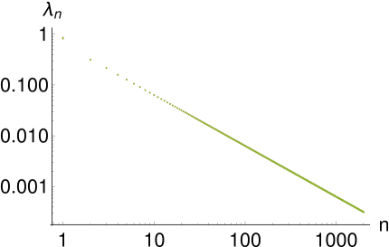
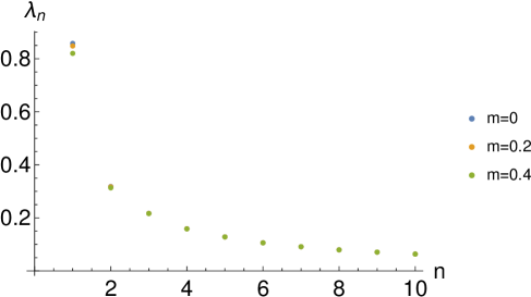
(a) (b)

Figure 1: (a):A log-log plot of the SJ eigenvalues $\lambda_{n}$ vs $n$ for $m=0,0.2$ and $0.4$, (b): a plot of $\lambda_{n}$ vs $n$ for small $n$. As one can see, the eigenvalues for $m=0.2$ and $0.4$ are barely distinguishable from $m=0$, except for the very smallest $n$ values.

3.1 Details of the calculations of SJ modes

We now show the calculation in broad strokes below, leaving some of the details to the Appendix A. We begin by reviewing the massless case. Here $Z_{l}(u,v)$ reduces to $u^{l}$ and $U_{a}(u,v)$ to $e^{au}$.

Operating $i\hat{\Delta}$ on $u^{l}$ or $v^{l}$ we find that

$$i\hat{\Delta}_{m=0}\circ u^{l} = \frac{iL^{2}}{2(l+1)}\left(\left(1+(-1)^{l+1}\right)-v\left(1-(-1)^{l+1}\right)-2u^{l+1}\right),$$

$$i\hat{\Delta}_{m=0}\circ v^{l} = \frac{iL^{2}}{2(l+1)}\left(\left(1+(-1)^{l+1}\right)-u\left(1-(-1)^{l+1}\right)-2v^{l+1}\right),$$ (35)

while on the plane wave modes

$$i\hat{\Delta}_{m=0}\circ e^{iku} = -\frac{L^{2}}{k}\left(e^{iku}-\cos(k)+iv\sin(k)\right),$$

$$i\hat{\Delta}_{m=0}\circ e^{ikv} = -\frac{L^{2}}{k}\left(e^{ikv}-\cos(k)+iu\sin(k)\right).$$ (36)

Here, $k$ takes on all values including $k=0$, which is the constant solution. From the antisymmetric combination

$$i\hat{\Delta}_{m=0}\circ\left(e^{iku}-e^{ikv}\right)=-\frac{L^{2}}{k}\left(e^{iku}-e^{ikv}-i\sin(k)(u-v)\right),$$ (37)

we find the first set of massless eigenfunctions

$$u_{k}^{A(0)}(u,v)\equiv e^{iku}-e^{ikv}$$ (38)

with $k\in\mathcal{K}_{f}$ satisfying the quantization condition

$$\sin(k)=0\;\text{or}\;k=n\pi.$$ (39)

with eigenvalues $-\frac{L^{2}}{k}$. The symmetric combination on the other hand gives

$$i\hat{\Delta}_{m=0}\circ\left(e^{iku}+e^{ikv}\right)=-\frac{L^{2}}{k}\left(e^{iku}+e^{ikv}-2\cos(k)\right)-\frac{iL^{2}}{k}\sin(k)(u+v).$$ (40)

Since the symmetric eigenfunction can include a constant piece and noting that

$$\hat{\Delta}_{m=0}\circ c=-icL^{2}(u+v),$$ (41)

we find the second set of eigenfunctions

$$u_{k}^{S(0)}(u,v)\equiv e^{iku}+e^{ikv}-2\cos(k)$$ (42)

with eigenvalue $-\frac{L^{2}}{k}$, where $k\in\mathcal{K}_{g}$ satisfies

$$\sin(k)=2k\cos(k).$$ (43)

$\{u_{k}^{A(0)}\}$ and $\{u_{k}^{S(0)}\}$ together form a complete set of eigenfunctions of $i\Delta$ as can be shown by [4].

This sets the stage for the calculation of the massive SJ modes. We begin by again looking the action of $i\hat{\Delta}$ on the solutions $Z_{l}(u,v)$ and $U_{a}(u,v)$,

$$i\hat{\Delta}\circ Z_{l}(u,v) = \frac{iL^{2}}{2}\sum_{j,s=0}^{\infty}\frac{(-1)^{j+s}m^{2(j+s)}l!}{2^{l+s}(j!)^{2}s!(s+l)!}\Omega^{l}_{js},$$ (44)

$$i\hat{\Delta}\circ U_{a}(u,v) = \frac{iL^{2}}{2}U_{a}(u,v)\sum_{j,s=0}^{\infty}\frac{(-1)^{j}m^{2(j+s)}}{2^{j+s}(j!)^{2}s!a^{s}}\Delta^{a}_{js}(u,v),$$ (45)

where

$$\Omega^{l}_{js}(u,v) \equiv \biggl{(}\int_{-}dp\,dq-\int_{+}dp\,dq\biggr{)}p^{j}q^{j}(u-p)^{l+s}(v-q)^{s},$$

$$\Delta^{a}_{js}(u,v) \equiv \biggl{(}\int_{-}dp\,dq-\int_{+}dp\,dq\biggr{)}p^{j}q^{j+s}e^{-ap}.$$ (46)

It is useful to re-express Eqn. (45) as

$$i\hat{\Delta}\circ U_{a}(u,v)=\frac{iL^{2}}{2}U_{a}(u,v)\sum_{n=0}^{\infty}m^{2n}A_{a,n}(u,v),$$ (47)

where

$$A_{a,n}(u,v)\equiv\sum_{j=0}^{n}\frac{(-1)^{j}}{2^{n}(j!)^{2}(n-j)!a^{(n-j)}}\Delta^{a}_{j(n-j)}(u,v).$$ (48)

This gives

$$i\hat{\Delta}\circ U_{a}(u,v)=-\frac{iL^{2}}{a}U_{a}(u,v)-\frac{iL^{2}}{a}\sum_{n=0}^{\infty}m^{2n}\mathcal{F}_{a,n}(u,v),$$ (49)

where

$$\mathcal{F}_{a,n}(u,v)\equiv F_{a,n}(u,v)\sinh(a)+G_{a,n}(u,v)\cosh(a),$$ (50)

with

$$F_{a,n}(u,v) \equiv \sum_{s=0}^{n}\sum_{j=0}^{s}\sum_{l=0}^{j}\frac{(-1)^{n-s+j}v^{n-s}\left((u+1)^{j-l}(v+1)^{s+1}+(u-1)^{j-l}(v-1)^{s+1}\right)}{2^{n+1}a^{n-j+l}(n-s)!j!(s-j)!(j-l)!(s+1)},$$

$$G_{a,n}(u,v) \equiv \sum_{s=0}^{n}\sum_{j=0}^{s}\sum_{l=0}^{j}\frac{(-1)^{n-s+j}v^{n-s}\left((u-1)^{j-l}(v-1)^{s+1}-(u+1)^{j-l}(v+1)^{s+1}\right)}{2^{n+1}a^{n-j+l}(n-s)!j!(s-j)!(j-l)!(s+1)}.$$ (51)

Our first guess, inspired by the massless calculation, is that in order to find the SJ modes, we will need the antisymmetrized and symmetrized versions of Eqns (44) and (47), which we denote by $A/S$. As noted above, and is evident from Eqn. (49), in order to obtain the SJ modes, $U^{A/S}_{a}(u,v)$ must be supplemented by a function $H^{A/S}_{a}(u,v)$ made from the $Z_{l}(u,v)$.

Taking our cue from the massless case, let us assume that such a function exists, i.e.,

$$i\hat{\Delta}\circ\left(U^{A/S}_{a}(u,v)+H^{A/S}_{a}(u,v)\right)=-\frac{iL^{2}}{a}\left(U^{A/S}_{a}(u,v)+H^{A/S}_{a}(u,v)\right),$$ (52)

where $k$ satisfies an appropriate quantization condition $\mathcal{K}^{A/S}$. Then, from Eqn. (49) $H^{A/S}_{a}(u,v)$ must satisfy

$$i\hat{\Delta}\circ H^{A/S}_{a}(u,v)+\frac{iL^{2}}{a}H^{A/S}_{a}(u,v)-\frac{iL^{2}}{a}\sum_{n=0}^{\infty}m^{2n}\mathcal{F}^{A/S}_{a,n}(u,v)=0.$$ (53)

Up to now the discussion has been general. If the expressions above could be calculated in closed form, then one would be able to solve the SJ mode problem for any mass $m$. It is unclear how to proceed to do this, except order by order in $m^{2}$.

We now demonstrate this explicitly up to $\mathcal{O}(m^{4})$. We begin by taking $a=ik$ and writing Eqn. (49) as

$$i\hat{\Delta}\circ U^{A/S}_{ik}(u,v)\approx-\frac{L^{2}}{k}U^{A/S}_{ik}(u,v)-\frac{L^{2}}{k}\left(i\sin(k)\sum_{n=0}^{\infty}m^{2n}F^{A/S}_{ik,n}(u,v)+\cos(k)\sum_{n=0}^{\infty}m^{2n}G^{A/S}_{ik,n}(u,v)\right),$$ (54)

where the expressions for $F_{ik,n}(u,v)$ and $G_{ik,n}(u,v)$ for different $n$ have been calculated in Appendix A. The function $H^{A/S}_{k}(u,v)$ must therefore satisfy

$$i\hat{\Delta}\circ H^{A/S}_{ik}(u,v)+\frac{L^{2}}{k}\left(H^{A/S}_{ik}(u,v)-i\sin(k)\sum_{n=0}^{\infty}m^{2n}F^{A/S}_{ik,n}(u,v)-\cos(k)\sum_{n=0}^{\infty}m^{2n}G^{A/S}_{ik,n}(u,v)\right)=0.$$ (55)

From the result for the massless case, we expect the quantization condition for $k$ to be of the general form

$$\sin(k)=\cos(k)\sum_{n=0}^{\infty}m^{2n}Q^{A/S}_{n}(k),$$ (56)

with $Q^{A}_{0}(k)=0$ and $Q^{S}_{0}(k)=2k$. Inserting this into Eqn. (55) gives

$$i\hat{\Delta}\circ H^{A/S}_{ik}(u,v)+\frac{L^{2}}{k}H^{A/S}_{ik}(u,v)-\frac{L^{2}}{k}\cos(k)\left(\sum_{n=0}^{\infty}m^{2n}P^{A/S}_{n}(u,v)\right)=0,$$ (57)

where

$$P^{A/S}_{n}(u,v)\equiv G^{A/S}_{n}(u,v)+i\sum_{j=0}^{n}Q^{A/S}_{j}(k)F^{A/S}_{n-j}(u,v).$$ (58)

The challenge is therefore to obtain the explicit form for these expressions. Finding a general expression in this manner is very challenging, but we will now show that it can be found to $\mathcal{O}(m^{4})$.

Since the $H^{A/S}_{a}(u,v)$ must be constructed from the $Z_{l}(u,v)$, we are interested in the action of $i\hat{\Delta}$ on $Z_{l}(u,v)$ up to $\mathcal{O}(m^{4})$ i.e.,

$$i\hat{\Delta}\circ Z_{l}(u,v)=\frac{iL^{2}}{2}\sum_{j,s,j+s\leq 2}\frac{(-1)^{j+s}m^{2(j+s)}l!}{2^{l+s}(j!)^{2}s!(s+l)!}\Omega^{l}_{js}+\mathcal{O}(m^{6}).$$ (59)

We calculate this expression for $l=0,1,2$, up to $\mathcal{O}(m^{4})$ in the Appendix A. Using the expression of $P_{n}^{A}(u,v)$ given in Appendix A, we find that up to $\mathcal{O}(m^{4})$ the antisymmetric version of Eqn. (57) reduces to

$$\left(i\hat{\Delta}+\frac{L^{2}}{k}\right)\circ\left(H^{A}_{ik}(u,v)+\cos(k)\left(\left(\frac{im^{2}}{2k}-\frac{im^{4}(6+k^{2})}{24k^{3}}\right)Z^{A}_{1}(u,v)-\frac{m^{4}}{4k^{2}}Z^{A}_{2}(u,v)\right)\right)\approx 0.$$ (60)

Therefore

$$u^{A}_{k}(u,v)=U^{A}_{ik}(u,v)-\cos(k)\left(\left(\frac{im^{2}}{2k}-\frac{im^{4}(6+k^{2})}{24k^{3}}\right)Z^{A}_{1}(u,v)-\frac{m^{4}}{4k^{2}}Z^{A}_{2}(u,v)\right)+\mathcal{O}(m^{6}),$$ (61)

with eigenvalue $-\frac{L^{2}}{k}$ with $k\in\mathcal{K}_{A}$ satisfying the quantization condition

$$\sin(k)=\left(\frac{m^{2}}{k}+\frac{m^{4}}{12k}\left(1-\frac{3}{k^{2}}\right)\right)\cos(k)+\mathcal{O}(m^{6}).$$ (62)

Similarly using the expression of $P_{n}^{S}(u,v)$ given in Appendix A and after more painstaking algebra, we find that Eqn. (57) can be written as

$$\left(i\hat{\Delta}+\frac{L^{2}}{k}\right)\circ\left(H^{S}_{ik}(u,v)+\cos(k)\left(\left(1+\frac{m^{2}}{2}-\frac{m^{4}}{8k^{2}}(2-9k^{2})\right)Z^{S}_{0}(u,v)\right.\right.$$

$$\left.\left.+\left(\frac{3im^{2}}{2k}-\frac{im^{4}}{24k^{3}}(6-31k^{2})\right)Z^{S}_{1}(u,v)-\frac{m^{4}}{8k^{2}}(4-k^{2})Z^{S}_{2}(u,v)\right)\right)\approx 0.$$ (63)

Therefore the symmetric eigenfunction is

$$u^{S}_{k}(u,v) = U^{S}_{ik}(u,v)-\cos(k)\left(\left(1+\frac{m^{2}}{2}-\frac{m^{4}}{8k^{2}}(2-9k^{2})\right)Z^{S}_{0}(u,v)\right.$$ (64)

$$\left.+\left(\frac{3im^{2}}{2k}-\frac{im^{4}}{24k^{3}}(6-31k^{2})\right)Z^{S}_{1}(u,v)-\frac{m^{4}}{8k^{2}}(4-k^{2})Z^{S}_{2}(u,v)\right)+\mathcal{O}(m^{6}),$$

with eigenvalue $-\frac{L^{2}}{k}$, where $k\in\mathcal{K}_{S}$ satisfies

$$\sin(k)=\left(2k-\frac{m^{2}}{k}(1-2k^{2})+\frac{m^{4}}{12k^{3}}(3-29k^{2}+28k^{4})\right)\cos(k)+\mathcal{O}(m^{6}).$$ (65)

Unfortunately, the structure of neither the coefficients in $u^{A/S}_{k}$ nor the quantization condition are enough to suggest a generalization to all orders. One could of course proceed to the next order $\mathcal{O}(m^{6})$ but the calculation gets prohibitively more complex.

3.2 Completeness of the eigenfunctions

We now show that the eigenfunctions $\{u_{k}^{A}|k\in\mathcal{K}_{A}\}$ and $\{u_{k}^{S}|k\in\mathcal{K}_{S}\}$ form a complete set of eigenfunctions of $i\Delta$. If this is the case, then we can decompose $i\Delta$ as

$$i\Delta(u,v;u^{\prime},v^{\prime})=\sum_{k\in\mathcal{K}_{A}}-\frac{L^{2}}{k}u^{A}_{k}(u,v){u^{A}_{k}}^{*}(u^{\prime},v^{\prime})+\sum_{k\in\mathcal{K}_{S}}-\frac{L^{2}}{k}u^{S}_{k}(u,v){u^{S}_{k}}^{*}(u^{\prime},v^{\prime})+\mathcal{O}(m^{6}),$$ (66)

which implies that

$$\int_{S}du\,dv\,du^{\prime}\,dv^{\prime}|\Delta(u,v;u^{\prime},v^{\prime})|^{2}=\sum_{k\in\mathcal{K}_{A}}\biggl{(}\frac{L^{2}}{k}\biggr{)}^{2}+\sum_{k\in\mathcal{K}_{S}}\biggl{(}\frac{L^{2}}{k}\biggr{)}^{2}+\mathcal{O}(m^{6}).$$ (67)

To $\mathcal{O}(m^{4})$ the LHS of Eqn. (67) reduces to

$$\frac{L^{4}}{4}\int_{-1}^{1}dudv\left(\int_{-}dp\,dq+\int_{+}dp\,dq\right)J_{0}^{2}\left(m\sqrt{2pq}\right)$$ (68)

$$= \frac{L^{4}}{4}\int_{-1}^{1}dudv\left(\int_{-}dp\,dq+\int_{+}dp\,dq\right)\left(1-m^{2}pq+\frac{3}{8}m^{4}p^{2}q^{2}\right)+\mathcal{O}(m^{6})$$

$$= 2L^{4}\left(1-\frac{4}{9}m^{2}+\frac{1}{6}m^{4}\right)+\mathcal{O}(m^{6}).$$

For the RHS $k\in\mathcal{K}_{A/S}$, we make use of the expansion $k^{A/S}\approx k^{A/S}_{0}+m^{2}k^{A/S}_{1}+m^{4}k^{A/S}_{2}$. For the antisymmetric quantization condition Eqn. (30) since $k_{0}^{A}=n\pi$ this gives, up to $\mathcal{O}(m^{4})$

$$m^{2}k_{1}^{A}+m^{4}k_{2}^{A}=\frac{m^{2}}{k_{0}^{A}}\left(1-m^{2}\frac{k_{1}^{A}}{k_{0}^{A}}\right)-\frac{m^{4}}{4{k_{0}^{A}}^{3}}+\frac{m^{4}}{12k_{0}^{A}}+\mathcal{O}(m^{6}).$$ (69)

Solving the above equation for different orders of $m^{2}$, we get

$$k_{1}^{A} = \frac{1}{n\pi},$$ (70)

$$k_{2}^{A} = \frac{1}{12n\pi}-\frac{5}{4n^{3}\pi^{3}},$$ (71)

so that

$$\sum_{k\in\mathcal{K}_{A}}L^{4}\frac{1}{k^{2}} = 2L^{4}\sum_{n=1}^{\infty}\frac{1}{n^{2}\pi^{2}}\left(1-2m^{2}\frac{1}{n^{2}\pi^{2}}-m^{4}\left(\frac{1}{6n^{2}\pi^{2}}-\frac{11}{2n^{4}\pi^{4}}\right)\right)+\mathcal{O}(m^{6})$$ (72)

$$= 2L^{4}\left(\frac{1}{6}-\frac{m^{2}}{45}+\frac{m^{4}}{252}\right)+\mathcal{O}(m^{6}).$$

For the symmetric contribution Eqn. (33) up to $\mathcal{O}(m^{4})$ we have

$$\sum_{n=0}^{2}m^{2n}K_{n}(k^{S}_{0},k^{S}_{1},k^{S}_{2})+\mathcal{O}(m^{6})=0,$$ (73)

where

$$K_{1}(k^{S}_{0},k^{S}_{1},k^{S}_{2}) = \sin(k^{S}_{0})-2k^{S}_{0}\cos(k^{S}_{0}),$$

$$K_{2}(k^{S}_{0},k^{S}_{1},k^{S}_{2}) = \left(\frac{2{k^{S}_{0}}^{2}-1+k^{S}_{1}k^{S}_{0}}{k^{S}_{0}}\right)\cos(k^{S}_{0})-2k^{S}_{1}k^{S}_{0}\sin(k^{S}_{0}),$$

$$K_{3}(k^{S}_{0},k^{S}_{1},k^{S}_{2}) = \left(\frac{3-29{k^{S}_{0}}^{2}+28{k^{S}_{0}}^{4}+12k^{S}_{1}k^{S}_{0}}{12{k^{S}_{0}}^{3}}+2k^{S}_{1}+k^{S}_{2}-{k^{S}_{1}}^{2}k^{S}_{2}\right)\cos(k^{S}_{0})$$ (74)

$$+\left(\frac{k^{S}_{1}-2k^{S}_{1}k^{S}_{0}-2{k^{S}_{0}}^{3}}{k^{S}_{0}}-\frac{3}{2}{k^{S}_{1}}^{2}\right)\sin(k^{S}_{0}).$$

Equating the above order by order in $m^{2}$, we get

$$\sin(k^{S}_{0}) = 2k^{S}_{0}\cos(k^{S}_{0}),$$ (75)

$$k^{S}_{1} = \frac{1-2{k^{S}_{0}}^{2}}{k^{S}_{0}(1-4{k^{S}_{0}}^{2})},$$ (76)

$$k^{S}_{2} = \frac{(3-4{k^{S}_{0}}^{2})(-5+35{k^{S}_{0}}^{2}-40{k^{S}_{0}}^{4}+16{k^{S}_{0}}^{6})}{12{k^{S}_{0}}^{3}(1-4{k^{S}_{0}}^{2})^{3}}.$$ (77)

$$\sum_{k\in\mathcal{K}_{S}}L^{4}\frac{1}{k^{2}} = 2L^{4}\sum_{k^{S}_{0}\in\mathcal{K}_{g}}\left(\frac{1}{{k^{S}_{0}}^{2}}-2m^{2}\left(\frac{1}{{k^{S}_{0}}^{4}}+\frac{2}{{k^{S}_{0}}^{2}}-\frac{8}{4{k^{S}_{0}}^{2}-1}\right)\right.$$

$$\left.+m^{4}\left(\frac{11}{2{k^{S}_{0}}^{6}}+\frac{127}{6{k^{S}_{0}}^{4}}+\frac{280}{3{k^{S}_{0}}^{2}}+\frac{32}{(4{k^{S}_{0}}^{2}-1)^{3}}+\frac{32}{(4{k^{S}_{0}}^{2}-1)^{2}}-\frac{1120}{3(4{k^{S}_{0}}^{2}-1)}\right)\right)+\mathcal{O}(m^{6}).$$

We evaluate the above series by using the method developed in [13] and used in [3, 4], details of which can be found in Appendix B. This leads to

$$\sum_{k^{S}_{0}\in\mathcal{K}_{g}}\frac{1}{{k^{S}_{0}}^{2}}=\frac{5}{6}\;\;,\;\;\;\sum_{k^{S}_{0}\in\mathcal{K}_{g}}\frac{1}{{k^{S}_{0}}^{4}}=\frac{49}{90}\;\;\text{and}\;\;\;\sum_{k^{S}_{0}\in\mathcal{K}_{g}}\frac{1}{{k^{S}_{0}}^{6}}=\frac{377}{945}$$ (79)

and

$$\sum_{k^{S}_{0}\in\mathcal{K}_{g}}\frac{1}{4{k^{S}_{0}}^{2}-1} = \frac{1}{4},$$

$$\sum_{k^{S}_{0}\in\mathcal{K}_{g}}\frac{1}{(4{k^{S}_{0}}^{2}-1)^{2}} = -\frac{1}{4}\left(\frac{\cos(1/2)-2\sin(1/2)}{\cos(1/2)-\sin(1/2)}\right),$$

$$\sum_{k^{S}_{0}\in\mathcal{K}_{g}}\frac{1}{(4{k^{S}_{0}}^{2}-1)^{3}} = \frac{1}{64}\left(1+\frac{19\cos(1/2)-35\sin(1/2)}{\cos(1/2)-\sin(1/2)}\right).$$ (80)

This simplifies Eqn. (LABEL:eqn:gcomp) to

$$\sum_{k\in\mathcal{K}_{S}}2L^{4}\frac{1}{k^{2}}=2L^{4}\left(\frac{5}{6}-\frac{19}{45}m^{2}+\frac{41}{252}m^{4}\right)+\mathcal{O}(m^{6}).$$ (81)

Adding the contributions from the antisymmetric and symmetric eigenfunctions the RHS of Eqn. (67) reduces to

$$\sum\lambda_{k}^{2}=2L^{4}\left(1-\frac{4}{9}m^{2}+\frac{1}{6}m^{4}\right)+\mathcal{O}(m^{6}),$$ (82)

which is same as its LHS. Thus, to $\mathcal{O}(m^{4})$ the $u^{A/S}_{k}$ are a complete set of eigenfunctions of $i\hat{\Delta}$.

4 The Wightman function: the small mass limit

We can now write down the formal expression for the SJ Wightman function to $\mathcal{O}(m^{4})$ using the SJ modes obtained above, as

$$W_{SJ}(u,v,u^{\prime},v^{\prime})=\sum_{k\in\mathcal{K}_{A},\,k<0}-\frac{L^{2}}{k}\frac{u^{A}_{k}(u,v){u^{A}_{k}}^{*}(u^{\prime},v^{\prime})}{||u_{k}^{A}||^{2}}+\sum_{k\in\mathcal{K}_{S},\,k<0}-\frac{L^{2}}{k}\frac{u^{S}_{k}(u,v){u^{S}_{k}}^{*}(u^{\prime},v^{\prime})}{||u_{k}^{S}||^{2}}+\mathcal{O}(m^{6}),$$ (83)

where $\mathcal{K}_{A/S}$ denote the positive SJ eigenvalues. In particular $k=-k_{A}(n)$ with $n\in{\mathbb{Z}}^{+}$ (Eqn. (31)) and $k=-k_{S}(k_{0})$ with $k_{0}$ satisfying $\tan(k_{0})=2k_{0}$ (Eqn. (34)). Here $||u^{A/S}_{k}||$ denotes the $\mathcal{L}^{2}$ norm of the modes $u^{A/S}_{k}$

$$||u^{A/S}_{k}||^{2}=L^{2}\int_{-1}^{1}du\int_{-1}^{1}dvu^{A/S}_{k}(u,v){u^{A/S}_{k}}^{*}(u,v).$$ (84)

For $k=-k_{A}(n)$

$$||u^{A}_{k}||^{2}=8L^{2}\left(1+\frac{m^{2}}{n^{2}\pi^{2}}+\frac{m^{4}}{n^{2}\pi^{2}}\left(\frac{1}{12}-\frac{11}{4n^{2}\pi^{2}}\right)\right)+\mathcal{O}(m^{6}).$$ (85)

In the symmetric case, $k=-k_{S}(k_{0})$ the quantization condition is complicated. Following [3], we make the approximation

$$k_{S}(n)\approx\left(n-\frac{1}{2}\right)\pi,\,\,n\in{\mathbb{Z}}^{+}.$$ (86)

As shown in Fig. 2, we see that except for the first few modes this is a good approximation, and in fact improves with increasing mass. This approximation in the quantization condition makes $\cos(k_{S})=0$, thus simplifying $u^{S}_{k}(u,v)$ to

$$u^{S}_{-k_{S}}(u,v)=U^{S}_{-ik_{S}}(u,v)\Rightarrow||u^{S}_{k_{S}}||=8L^{2}.$$ (87)

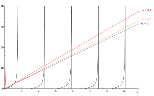
Figure 2: Plot of the quantization condition, Eqn. (33) for the symmetric SJ modes for m=0,0.2 and 0.4, where $k_{S}>0$.

We examine the antisymmetric and symmetric contributions to $W_{SJ}$ separately

$$W_{SJ}=W_{SJ}^{A}+W_{SJ}^{S}.$$ (88)

For the antisymmetric contribution, using the quantization condition $k=-k_{A}(n)$ and the simplification Eqn. (85) for the norm

$$W_{SJ}^{A}(u,v,u^{\prime},v^{\prime})=\sum_{n=1}^{\infty}\frac{1}{8n\pi}\left(1-\frac{2m^{2}}{n^{2}\pi^{2}}+\frac{m^{4}}{n^{2}\pi^{2}}\left(\frac{7}{n^{2}\pi^{2}}-\frac{1}{6}\right)\right)u^{A}_{k}(u,v)u_{k}^{A*}(u^{\prime},v^{\prime})+\mathcal{O}(m^{6}).$$ (89)

To leading order $u^{A}_{k}$ can be re-expressed as

$$u^{A}_{k}(u,v) = e^{-in\pi u}-e^{-in\pi v}+\Psi_{A}(n,u,v)+\mathcal{O}(m^{6}),$$

$$\Psi_{A}(n,u,v) = \sum_{j=1}^{3}\left(\frac{(-1)^{n}f_{j}(m;u,v)}{n^{j}}+\frac{g_{j}(m;u,v)e^{-in\pi u}}{n^{j}}-\frac{g_{j}(m;v,u)e^{-in\pi v}}{n^{j}}\right),$$ (90)

where

$$f_{1}(m;u,v)\equiv\frac{im^{2}}{2\pi}(u-v)-\frac{im^{4}}{24\pi}(u-v)(1+3uv), g_{1}(m;u,v)\equiv-\frac{im^{2}(2u+v)}{2\pi}-\frac{im^{4}u}{12\pi},$$

$$f_{2}(m;u,v)\equiv-\frac{m^{4}}{4\pi^{2}}(u^{2}-v^{2}), g_{2}(m;u,v)\equiv-\frac{m^{4}(2u+v)^{2}}{8\pi^{2}},$$

$$f_{3}(m;u,v)\equiv-\frac{3im^{4}}{4\pi^{3}}(u-v), g_{3}(m;u,v)\equiv\frac{im^{4}(15u+6v)}{12\pi^{3}}.$$ (91)

We further split

$$W_{SJ}^{A}=A_{\mathrm{I}}+A_{\mathrm{II}}+A_{\mathrm{III}}+A_{\mathrm{IV}}+\mathcal{O}(m^{6}),$$ (92)

where

$$A_{\mathrm{I}} \equiv \sum_{n=1}^{\infty}\frac{1}{8n\pi}\left(1-\frac{2m^{2}}{n^{2}\pi^{2}}+\frac{m^{4}}{n^{2}\pi^{2}}\left(\frac{7}{n^{2}\pi^{2}}-\frac{1}{6}\right)\right)\left(e^{-in\pi u}-e^{-in\pi v}\right)\left(e^{in\pi u^{\prime}}-e^{in\pi v^{\prime}}\right),$$

$$A_{\mathrm{II}} \equiv \sum_{n=1}^{\infty}\frac{1}{8n\pi}\left(1-\frac{2m^{2}}{n^{2}\pi^{2}}\right)\left(e^{-in\pi u}-e^{-in\pi v}\right)\Psi_{A}^{*}(n,u^{\prime},v^{\prime}),$$

$$A_{\mathrm{III}} \equiv \sum_{n=1}^{\infty}\frac{1}{8n\pi}\left(1-\frac{2m^{2}}{n^{2}\pi^{2}}\right)\Psi_{A}(n,u,v)\left(e^{in\pi u^{\prime}}-e^{in\pi v^{\prime}}\right),$$

$$A_{\mathrm{IV}} \equiv \sum_{n=1}^{\infty}\frac{1}{8n\pi}\Psi_{A}(n,u,v)\Psi_{A}^{*}(n,u^{\prime},v^{\prime}).$$

These terms can be further simplified to $\mathcal{O}(m^{4})$ as we have shown in Appendix. C.

For the symmetric contribution $W_{SJ}^{S}$ we use the simplification Eqns (86) and (87) to express

$$W_{SJ}^{S}=\sum_{n=1}^{\infty}\frac{1}{4\pi(2n-1)}U^{S}_{-ik_{S}}(u,v){U^{S}}_{-ik_{S}}^{*}(u^{\prime},v^{\prime})+\epsilon_{m}(u,v,u^{\prime},v^{\prime})+\mathcal{O}(m^{6}).$$ (94)

Here $\epsilon_{m}(u,v;u^{\prime},v^{\prime})$ is the correction term coming from the approximation of the quantization condition Eqn. (86). This is analytically difficult to obtain and in Sec. 4.3, we will evaluate it numerically for different values of $m$.

Using the $\mathcal{O}(m^{4})$ expansion of $U_{-ik}$ from Eqn. (17), we write $U_{-ik_{S}}^{S}$ as

$$U_{-ik_{S}(n)}^{S}(u,v) = \left(e^{-i\left(n-\frac{1}{2}\right)\pi u}+e^{-i\left(n-\frac{1}{2}\right)\pi v}\right)+\Psi_{S}(n,u,v)+\mathcal{O}(m^{6}),$$

$$\Psi_{S}(n,u,v) = -\frac{im^{2}}{(2n-1)\pi}\left(ve^{-i\left(n-\frac{1}{2}\right)\pi u}+ue^{-i\left(n-\frac{1}{2}\right)\pi v}\right)$$ (95)

$$\quad\quad\quad-\frac{m^{4}}{4(2n-1)^{2}\pi^{2}}\left(v^{2}e^{-i\left(n-\frac{1}{2}\right)\pi u}+u^{2}e^{-i\left(n-\frac{1}{2}\right)\pi v}\right).$$

Again for the symmetric part, we can write

$$W_{SJ}^{S}=S_{\mathrm{I}}+S_{\mathrm{II}}+S_{\mathrm{III}}+S_{\mathrm{IV}}+\epsilon_{m}(u,v,u^{\prime},v^{\prime})+\mathcal{O}(m^{6}),$$ (96)

where

$$S_{\mathrm{I}} \equiv \frac{1}{4\pi}\sum_{n=1}^{\infty}\frac{1}{2n-1}\left(e^{-i\left(n-\frac{1}{2}\right)\pi u}+e^{-i\left(n-\frac{1}{2}\right)\pi v}\right)\left(e^{i\left(n-\frac{1}{2}\right)\pi u^{\prime}}+e^{i\left(n-\frac{1}{2}\right)\pi v^{\prime}}\right),$$

$$S_{\mathrm{II}} \equiv \frac{1}{4\pi}\sum_{n=1}^{\infty}\frac{1}{2n-1}\left(e^{-i\left(n-\frac{1}{2}\right)\pi u}+e^{-i\left(n-\frac{1}{2}\right)\pi v}\right)\Psi_{S}^{*}(n,u^{\prime},v^{\prime}),$$

$$S_{\mathrm{III}} \equiv \frac{1}{4\pi}\sum_{n=1}^{\infty}\frac{1}{2n-1}\Psi_{S}(n,u,v)\left(e^{i\left(n-\frac{1}{2}\right)\pi u^{\prime}}+e^{i\left(n-\frac{1}{2}\right)\pi v^{\prime}}\right),$$

$$S_{\mathrm{IV}} \equiv \frac{1}{4\pi}\sum_{n=1}^{\infty}\frac{1}{2n-1}\Psi_{S}(n,u,v)\Psi_{S}^{*}(n,u^{\prime},v^{\prime}).$$ (97)

Using the following result

$$\sum_{n=1}^{\infty}\frac{e^{i\left(n-\frac{1}{2}\right)\pi x}}{(2n-1)^{j}}={\mathrm{Li}}_{j}\left(e^{i\pi\frac{x}{2}}\right)-\frac{1}{2^{j}}{\mathrm{Li}}_{j}\left(e^{i\pi x}\right),$$ (98)

$S_{\mathrm{I}},S_{\mathrm{II}},S_{\mathrm{III}}$ and $S_{\mathrm{IV}}$ can further be simplified up to $\mathcal{O}(m^{4})$ as we have shown in Appendix C. In particular, $S_{\mathrm{I}}$ can be written as

$$S_{\mathrm{I}}=\frac{1}{4\pi}\left(\tanh^{-1}\left(e^{-\frac{i\pi(u-u^{\prime})}{2}}\right)+\tanh^{-1}\left(e^{-\frac{i\pi(v-v^{\prime})}{2}}\right)+\tanh^{-1}\left(e^{-\frac{i\pi(u-v^{\prime})}{2}}\right)+\tanh^{-1}\left(e^{-\frac{i\pi(v-u^{\prime})}{2}}\right)\right).$$ (99)

Despite these simplifications in $W_{SJ}$, it is difficult to find a general closed form expression for $W_{SJ}$. Instead, as was done in [3], we focus on two subregions of $\mathcal{D}$, as shown in Fig. 3. In the center, far away from the boundary, one expects to obtain the Minkowski vacuum, while in the corner, one expects the Rindler vacuum. In the massless case studied by [3] the former expectation was shown to be the case. However, in the corner, instead of the Rindler vacuum, they found that that $W_{SJ}$ looks like the massless mirror vacuum. One of the main motivations to look at the massive case, is to compare with these results.

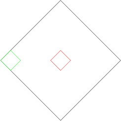
Figure 3: The center and corner regions in the causal diamond $\mathcal{D}$.

We now write down the expressions for the various vacua that we wish to compare with:

$$W^{\mathrm{mink}}_{0}(u,v;u^{\prime},v^{\prime}) = -\frac{1}{4\pi}\ln\left(\Lambda^{2}e^{2\gamma}|2\Delta u\Delta v|\right)-\frac{i}{4}\mathrm{sgn}(\Delta u+\Delta v)\theta(\Delta u\Delta v),$$ (100)

$$W^{\mathrm{mink}}_{m}(u,v;u^{\prime},v^{\prime}) = \frac{1}{2\pi}K_{0}\left(m\sqrt{-2\Delta u\Delta v+i(\Delta u+\Delta v)\epsilon}\right),$$ (101)

$$W^{\mathrm{rind}}_{0}(\eta,\xi,\eta^{\prime},\xi^{\prime}) = -\frac{1}{4\pi}\ln\left(\Lambda^{2}e^{2\gamma}|\Delta\eta^{2}-\Delta\xi^{2}|\right)-\frac{i}{4}\mathrm{sgn}(\Delta\eta)\theta(\Delta\eta^{2}-\Delta\xi^{2}),$$ (102)

$$W^{\mathrm{rind}}_{m}(\eta,\xi,\eta^{\prime},\xi^{\prime}) = W^{\mathrm{mink}}_{m}(u,v,u^{\prime},v^{\prime})-\frac{1}{2\pi}\int_{-\infty}^{\infty}\frac{dy}{\pi^{2}+y^{2}}K_{0}(m\gamma_{1}),$$ (103)

$$W^{\mathrm{mirror}}_{0}(u,v,u^{\prime},v^{\prime}) = W^{\mathrm{mink}}_{0}(u,v;u^{\prime},v^{\prime})-W^{\mathrm{mink}}_{0}(u,v;v^{\prime},u^{\prime}),$$ (104)

$$W^{\mathrm{mirror}}_{m}(u,v,u^{\prime},v^{\prime}) = W^{\mathrm{mink}}_{m}(u,v;u^{\prime},v^{\prime})-W^{\mathrm{mink}}_{m}(u,v;v^{\prime},u^{\prime}).$$ (105)

In the expression Eqn. (100) for the massless Minkowski vacuum, $\gamma$ is the Euler-Mascheroni constant and $\Lambda=0.462$ (obtained in [3] by comparing $W_{SJ}$ with $W^{\mathrm{mink}}_{0}$). In the expression Eqn. (101) for the massive Minkowski vacuum [14], $K_{0}$ is the modified Bessel function of the second kind, with $\epsilon$ a constant such that that $0<\epsilon\ll 1$. In the expressions Eqn. (102) and Eqn. (103) (see [15]) for the Rindler vacua, $\alpha$ is the acceleration parameter, with

$$\eta=\frac{1}{\alpha}\tanh^{-1}\left(\frac{u+v}{u-v}\right), \xi=\frac{1}{2\alpha}\ln\left(-2\alpha^{2}uv\right),$$

$$\Delta\eta=\eta-\eta^{\prime},\quad\Delta\xi=\xi-\xi^{\prime}, \gamma_{1}=\sqrt{\xi^{2}+\xi^{\prime 2}+2\xi\xi^{\prime}\cosh(y-\eta+\eta^{\prime})}.$$ (106)

4.1 The center

We now consider a small diamond ${\mathcal{D}}_{l}$ at the center of $\mathcal{D}$ with $l\ll 1$ where one expects $W_{SJ}$ to resemble $W^{\mathrm{mink}}_{m}$. For small $\Delta u,\Delta v$, $W^{\mathrm{mink}}_{m}$ can be written as

$$W^{\mathrm{mink}}_{m}(u,v;u^{\prime},v^{\prime})\approx-\frac{1}{4\pi}\ln\left(\frac{m^{2}e^{2\gamma}}{2}\left|\Delta u\Delta v\right|\right)-\frac{i}{4}\mathrm{sgn}(\Delta u+\Delta v)\theta(\Delta u\Delta v)J_{0}\left(m\sqrt{2\Delta u\Delta v}\right).$$ (107)

To leading logarithmic order this is similar in form to $W^{\mathrm{mink}}_{0}$ (Eqn. (100)), with $m$ replaced by $2\Lambda$. We plot these functions in Fig. 4. For $m\ll\Lambda$ the real part of $W^{\mathrm{mink}}_{m}$ is larger than $W^{\mathrm{mink}}_{0}$ and for $m\gg\Lambda$ it is smaller. When $m_{c}=2\Lambda$, the two coincide in this approximation.

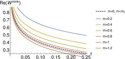
Figure 4: Plot of ${\mathrm{Re}}(W^{\mathrm{mink}}_{0})$ and ${\mathrm{Re}}(W^{\mathrm{mink}}_{m})$ vs the proper time ($\tau$)

Let us begin with $W_{SJ}^{A}$, Eqns (92) and (LABEL:eq:aone). As shown in Appendix C, the expressions for $A_{\mathrm{I}},A_{\mathrm{II}},A_{\mathrm{III}}$ and $A_{\mathrm{IV}}$ can be written in terms of Polylogarithms ${\mathrm{Li}}_{s}(x)$. For small $x$, i.e., near the center of $\mathcal{D}$ they simplify for the $s=1,3$ and $5$ to

$${\mathrm{Li}}_{1}\left(e^{i\pi x}\right) = -\ln(-i\pi x)-\frac{i\pi x}{2}+\frac{\pi^{2}x^{2}}{24}+\mathcal{O}(x^{3}),$$ (108)

$${\mathrm{Li}}_{3}\left(e^{i\pi x}\right) = \zeta(3)+\frac{i\pi^{3}x}{6}+\left(-\frac{3\pi^{2}}{4}+\frac{\pi^{2}}{2}\ln(-i\pi x)\right)x^{2}+\mathcal{O}(x^{3}),$$ (109)

$${\mathrm{Li}}_{5}\left(e^{i\pi x}\right) = \zeta(5)+\frac{i\pi^{5}x}{90}-\frac{\pi^{2}\zeta(3)x^{2}}{2}+\mathcal{O}(x^{3}),$$ (110)

where $\zeta$ are the Riemann Zeta function and $x$ denotes $u$ or $v$. In the expression for $A_{\mathrm{I}}$, the constant and linear terms in $x$ cancel out, so that

$$A_{\mathrm{I}} = -\frac{1}{8\pi}\left(\ln(|u-u^{\prime}||v-v^{\prime}|)-\ln(|u-v^{\prime}||v-u^{\prime}|)-C_{1}\frac{i\pi}{2}\right)$$ (111)

$$-\left(\frac{\pi}{96}+\frac{3m^{2}}{8\pi}+\frac{m^{4}}{8\pi}\left(\frac{1}{4}-\frac{7\zeta(3)}{\pi^{2}}\right)\right)(u-v)(u^{\prime}-v^{\prime})$$

$$-\frac{m^{2}}{8\pi}\left(1+\frac{m^{2}}{12}\right)\left[(u-u^{\prime})^{2}\ln\left(-i\pi(u-u^{\prime})\right)+(v-v^{\prime})^{2}\ln\left(-i\pi(v-v^{\prime})\right)\right.$$

$$\left.-(u-v^{\prime})^{2}\ln\left(-i\pi(u-v^{\prime})\right)-(v-u^{\prime})^{2}\ln\left(-i\pi(v-u^{\prime})\right)\right]+\mathcal{O}(\Delta^{3}),$$

where $C_{1}=\mathrm{sgn}(u-u^{\prime})+\mathrm{sgn}(v-v^{\prime})-\mathrm{sgn}(u-v^{\prime})-\mathrm{sgn}(v-u^{\prime})$ and $\Delta$ collectively denotes either $u-u^{\prime},v-v^{\prime},v^{\prime}-u$ or $v-u^{\prime}$. For sufficiently small $x$, the logarithmic term dominates significantly over other terms, and hence in $\mathcal{D}_{l}$

$$A_{\mathrm{I}}=-\frac{1}{8\pi}\left(\ln(|u-u^{\prime}||v-v^{\prime}|)-\ln(|u-v^{\prime}||v-u^{\prime}|)-C_{1}\frac{i\pi}{2}\right)+\mathcal{O}(m^{2},\Delta^{2}),$$ (112)

where we have hidden all the mass dependence in the correction.

Next, $A_{\mathrm{II}},A_{\mathrm{III}}$ and $A_{\mathrm{IV}}$ also involve another set of Polylogarithms of the type ${\mathrm{Li}}_{s}(-e^{i\pi x})$ for $s\geq 2$ as well as ${\mathrm{Li}}_{s}(e^{i\pi x})$ for $s=2,3,4$, which are multiplied to the functions $g_{j}(m;u,v)$ and $f_{j}(m;u,v)$ given in Eqn. (91). The $g_{j}(m;u,v)$ and $f_{j}(m;u,v)$ themselves go to zero either linearly or quadratically with $u,v$. This second set of Polylogarithms, unlike the first in Eqn. (110), are strictly convergent as $x\rightarrow 0$. Hence the $A_{\mathrm{II}},A_{\mathrm{III}}$ and $A_{\mathrm{IV}}$ are strongly sub-dominant with respect to $A_{\mathrm{I}}$ so that

$$W_{SJ}^{A}(u,v,u^{\prime},v^{\prime})=-\frac{1}{8\pi}\left(\ln(|u-u^{\prime}||v-v^{\prime}|)-\ln(|u-v^{\prime}||v-u^{\prime}|)-C_{1}\frac{i\pi}{2}\right)+\mathcal{O}(m^{2},\Delta^{2}).$$ (113)

Here we note that while the mass correction is significant in the antisymmetric SJ modes, it becomes insignificant in $W_{SJ}^{A}$ in the center of the diamond, compared to the dominating logarithmic term. Thus we see that in the center of $\mathcal{D}$, $W_{SJ}^{A}$ is identical to the massless case found in [3].

We now turn to the symmetric part $W_{SJ}^{S}$, Eqns (96) and (97). The expressions for $S_{\mathrm{I}},S_{\mathrm{II}},S_{\mathrm{III}}$ and $S_{\mathrm{IV}}$ can again be written in terms of Polylogarithms ${\mathrm{Li}}_{s}(x)$ as shown in Appendix C. For $S_{\mathrm{I}}$ however, the form given in Eqn. (99) is easier to analyze. Noting that for small $x$

$$\tanh^{-1}\left(e^{i\pi x/2}\right)=-\frac{1}{2}\ln\left(\frac{-i\pi x}{4}\right)-\frac{\pi^{2}x^{2}}{96}+\mathcal{O}(x^{3}),$$ (114)

near the center of $\mathcal{D}$ we see that

$$S_{\mathrm{I}} = -\frac{1}{8\pi}\left[\ln(|u-u^{\prime}||v-v^{\prime}|)+\ln(|u-v^{\prime}||v-u^{\prime}|)+4\ln\left(\frac{\pi}{4}\right)-C_{2}\frac{i\pi}{2}\right]$$ (115)

$$-\frac{\pi}{384}\left((u-u^{\prime})^{2}+(u-v^{\prime})^{2}+(v-u^{\prime})^{2}+(v-v^{\prime})^{2}\right)+\mathcal{O}(\Delta^{3}),$$

where $C_{2}=\mathrm{sgn}(u-u^{\prime})+\mathrm{sgn}(v-v^{\prime})+\mathrm{sgn}(u-v^{\prime})+\mathrm{sgn}(v-u^{\prime})$. Since the logarithmic term dominates,

$$S_{\mathrm{I}}=-\frac{1}{8\pi}\left[\ln(|u-u^{\prime}||v-v^{\prime}|)+\ln(|u-v^{\prime}||v-u^{\prime}|)+4\ln\left(\frac{\pi}{4}\right)-C_{2}\frac{i\pi}{2}\right]+\mathcal{O}(\Delta^{2}).$$ (116)

Next, we see that $S_{\mathrm{II}},S_{\mathrm{III}}$ and $S_{\mathrm{IV}}$ involve a set of Polylogarithms of the type ${\mathrm{Li}}_{s}(e^{i\pi x}),$ for $s=2,3$, multiplied by linear and quadratic functions of $u,v,u^{\prime}$ and $v^{\prime}$. This set of Polylogarithms are in fact strictly convergent as $x\rightarrow 0$. Hence the $S_{\mathrm{II}},S_{\mathrm{III}}$ and $S_{\mathrm{IV}}$ are strongly sub-dominant, with respect to $S_{\mathrm{I}}$, so that

$$W_{SJ}^{S}(u,v,u^{\prime},v^{\prime}) = -\frac{1}{8\pi}\left[\ln(|u-u^{\prime}||v-v^{\prime}|)+\ln(|u-v^{\prime}||v-u^{\prime}|)+4\ln\left(\frac{\pi}{4}\right)-C_{2}\frac{i\pi}{2}\right]$$ (117)

$$\quad+\epsilon_{m}^{center}+\mathcal{O}(m^{2},\Delta^{2}),$$

where $\epsilon_{m}^{center}$ is the correction in the center coming from the approximation to the quantization condition Eqn. (86). We will determine this numerically in Section 4.3. Up to this mass correction $W_{SJ}^{S}$ resembles the massless case found in [3].

Putting these pieces together we find that

$$W_{SJ}^{center}(u,v,u^{\prime},v^{\prime})\approx-\frac{1}{4\pi}\ln|\Delta u\Delta v|-\frac{i}{4}\mathrm{sgn}(\Delta u+\Delta v)\theta(\Delta u\Delta v)-\frac{1}{2\pi}\ln\left(\frac{\pi}{4}\right)+\epsilon_{m}^{center}.$$ (118)

A direct comparison with $W^{\mathrm{mink}}_{0}$ gives

$$W_{SJ}^{center}(u,v,u^{\prime},v^{\prime})-W^{\mathrm{mink}}_{0}(u,v,u^{\prime},v^{\prime})\approx-\frac{1}{2\pi}\ln\left(\frac{\pi}{4}\right)+\epsilon_{m}^{center}+\frac{1}{4\pi}\ln\left(2\Lambda^{2}e^{2\gamma}\right),$$ (119)

where $\Lambda\approx 0.462$ is fixed by comparing the massless $W_{SJ}$ with $W^{\mathrm{mink}}_{0}$ as in [3].

4.2 The corner

We now consider either of the two spatial corners of the diamond, $\mathcal{D}_{c}\subset\mathcal{D}$ as shown in Fig. 3. We use the small $\Delta u,\Delta v$ form of $W^{\mathrm{mink}}_{m}$ to express

$$W^{\mathrm{mirror}}_{m}\approx-\frac{1}{4\pi}\ln\left|\frac{\Delta u\Delta v}{(u-v^{\prime})(v-u^{\prime})}\right|-\frac{i}{4}\mathrm{sgn}(\Delta u+\Delta v)\left(\theta(\Delta u\Delta v)-\theta((u-v^{\prime})(v-u^{\prime}))\right).$$ (120)

As in [3] we make the coordinate transformation

$$\{u,u^{\prime},v,v^{\prime}\}\rightarrow\{u_{c},u^{\prime}_{c},v_{c},v^{\prime}_{c}\}\equiv\{u-1,u^{\prime}-1,v+1,v^{\prime}+1\},$$ (121)

which brings the origin $(0,0)$ to the left corner of the diamond.

For $W_{SJ}^{A}$ (Eqn. (92) and Eqn. (LABEL:eq:aone)), we note that $A_{\mathrm{I}}$ is invariant under this coordinate transformation and hence given by Eqn. (112) near the origin of $\mathcal{D}_{c}$. In $A_{\mathrm{II}},A_{\mathrm{III}}$ and $A_{\mathrm{IV}}$ the constant terms cancel out and, similar to the center calculation, they goes to zero linearly with $u,v$ and hence are strongly sub-dominant with respect to $A_{\mathrm{I}}$. Therefore, in the corner, $W_{SJ}^{A}$ simplifies to

$$W_{SJ}^{A}(u,v,u^{\prime},v^{\prime})=-\frac{1}{8\pi}\left(\ln(|u-u^{\prime}||v-v^{\prime}|)-\ln(|u-v^{\prime}||v-u^{\prime}|)-C_{1}\frac{i\pi}{2}\right)+\mathcal{O}(m^{2},\Delta),$$ (122)

and the sub-dominant part is now linear in $\Delta$.

For $W_{SJ}^{S}$ (Eqn. (96) and Eqn. (97)), under the coordinate transformation

$$S_{\mathrm{I}}=\frac{1}{4\pi}\left(\tanh^{-1}\left(e^{-\frac{i\pi(u-u^{\prime})}{2}}\right)+\tanh^{-1}\left(e^{-\frac{i\pi(v-v^{\prime})}{2}}\right)-\tanh^{-1}\left(e^{-\frac{i\pi(u-v^{\prime})}{2}}\right)-\tanh^{-1}\left(e^{-\frac{i\pi(v-u^{\prime})}{2}}\right)\right).$$ (123)

In the corner $\mathcal{D}_{c}\subset\mathcal{D}$ this simplifies to

$$S_{\mathrm{I}} = \frac{1}{8\pi}\left[-\ln(|u-u^{\prime}||v-v^{\prime}|)+\ln(|u-v^{\prime}||v-u^{\prime}|)+C_{1}\frac{i\pi}{2}\right]$$ (124)

$$-\frac{\pi}{384}\left((u-u^{\prime})^{2}+(v-v^{\prime})^{2}-(u-v^{\prime})^{2}-(v-u^{\prime})^{2}\right)+\mathcal{O}(\Delta^{3}).$$

For sufficiently small $\Delta$, the logarithmic term dominates the other terms so that

$$S_{\mathrm{I}}=\frac{1}{8\pi}\left[-\ln(|u-u^{\prime}||v-v^{\prime}|)+\ln(|u-v^{\prime}||v-u^{\prime}|)+C_{1}\frac{i\pi}{2}\right]+\mathcal{O}(\Delta^{2}).$$ (125)

As in the center, $S_{\mathrm{II}}$ and $S_{\mathrm{III}}$ go to zero while

$$S_{\mathrm{IV}}=\frac{7\zeta(3)m^{4}}{8\pi^{3}}+\mathcal{O}(\Delta)\approx 0.034m^{4}.$$ (126)

Therefore in the corner we see that

$$W_{SJ}^{S}\approx\frac{1}{8\pi}\left[-\ln(|u-u^{\prime}||v-v^{\prime}|)+\ln(|u-v^{\prime}||v-u^{\prime}|)+C_{1}\frac{i\pi}{2}\right]+0.034m^{4}+\epsilon_{m}^{corner}$$ (127)

i.e., there is a mass correction to the massless $W_{SJ}^{S}$. $\epsilon_{m}^{corner}$ is, as in the center calculation, a small but finite term coming from the approximation to the quantization condition Eqn. (86), which we will evaluate numerically in Sec. 4.3.

Putting these pieces together we find that in the corner $W_{SJ}$ takes the form

$$W_{SJ}^{corner}(u,v,u^{\prime},v^{\prime}) \approx -\frac{1}{4\pi}\ln\left|\frac{\Delta u\Delta v}{(u-v^{\prime})(v-u^{\prime})}\right|-\frac{i}{4}\mathrm{sgn}(\Delta u+\Delta v)\left(\theta(\Delta u\Delta v)-\theta((u-v^{\prime})(v-u^{\prime}))\right)$$ (128)

$$+0.034m^{4}+\epsilon_{m}^{corner}.$$

A direct comparison with $W^{\mathrm{mirror}}_{m}$ Eqn (120) gives

$$W_{SJ}^{corner}(u,v,u^{\prime},v^{\prime})-W^{\mathrm{mirror}}_{m}(u,v,u^{\prime},v^{\prime})\approx 0.034m^{4}+\epsilon_{m}^{corner}.$$ (129)

4.3 Numerical simulations for determining $\epsilon_{m}$

The formal expansion of $W_{SJ}$ in terms of the SJ modes Eqn. (83) can be truncated and evaluated numerically in $\mathcal{D}$. Here we do not need to use the approximation of the quantization condition Eqn (86). This allows us to evaluate the ensuing corrections $\epsilon_{m}^{center},\epsilon_{m}^{corner}$ numerically, and thus quantify the comparisons of $W_{SJ}$ obtained in the center and corner of $\mathcal{D}$ with the standard vacua.

We begin with the $N^{\mathrm{th}}$ truncation $W_{SJ}^{t}$ of the series form of $W_{SJ}$ Eqn(83) in the full diamond $\mathcal{D}$ for $N=100,200,\ldots 1000$. Fig 5 shows an explicit convergence of $W_{SJ}^{t}$ for these values of $N$. For the plot we considered the pairs $(u,v)=(x,x)$ and $(u^{\prime},v^{\prime})=(-x,-x)$ for timelike separated points, and $(u,v)=(x,-x)$ and $(u^{\prime},v^{\prime})=(-x,x)$ for spacelike separated points. From this point onwards, we will consider $W_{SJ}^{t}$ for $N=1000$.

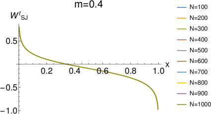
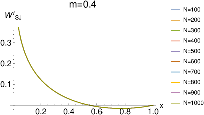
Figure 5: We show the convergence of the truncation of the series $W_{SJ}^{t}$ with $N$ for $m=0.2,0.4$ for timelike separated points (left) and spacelike separated points (right).

Next, we consider the difference $W_{SJ}^{t}-W_{SJ}^{t,approx}$ where the latter uses the approximation Eqn.  (86), both in the center and the corner of $\mathcal{D}$ in order to obtain $\epsilon_{m}^{center},\epsilon_{m}^{corner}$. It suffices to look at their symmetric parts $W_{SJ}^{S,t}$ since only these contribute (see Eqns (117), (127)). $\epsilon_{m}^{center}$ and $\epsilon_{m}^{corner}$ are not strictly constants. However, as we will see, they are approximately so. As in [3], they are evaluated by taking a set of randomly selected points in a small diamond in the center as well as in the corner. Here we take $10$ points and consider all $55$ pairs between them to calculate $\epsilon_{m}^{center},\epsilon_{m}^{corner}$. What we find in Fig. 6 is that they are very nearly equal and hence we can consider their average. The explicit averages for these masses are tabulated in Table 1 for future reference.

         

Figure 6: $\epsilon_{m}^{center}$ and $\epsilon_{m}^{corner}$ evaluated in a small diamond of $l=10^{-5}$ in the center and the corner of $\mathcal{D}$, for m=0,0.1,0.2,0.3 and 0.4. The standard deviation is very small and hence we can take $\epsilon_{m}^{center}$ and $\epsilon_{m}^{corner}$ to be approximately constant.

mass	$\epsilon_{m}^{center}$	$\epsilon_{m}^{corner}$
0	-0.0627	0
0.1	-0.0629	$-3.5\times 10^{-6}$
0.2	-0.0637	-0.00005
0.3	-0.0657	-0.00027
0.4	-0.0694	-0.00086

Table 1: A tabulation of $\epsilon_{m}^{center},\epsilon_{m}^{corner}$ for different $m$

This allows us to now compare $W_{SJ}$ calculated in the center Eqn (118) with $W^{\mathrm{mink}}_{0},W^{\mathrm{mink}}_{m}$. The difference with $W^{\mathrm{mink}}_{0}$ given in Eqn (119) is indeed very small. For $m=0.2$, for example,

$$W^{\mathrm{mink}}_{0}-W_{SJ}^{center}\simeq-\frac{1}{4\pi}\log(2\times 0.462^{2})-\frac{\gamma}{2\pi}-(-\frac{1}{2\pi}\log(\frac{\pi}{4})-\epsilon_{m}^{center})\simeq 0.001.$$ (130)

Similarly, in the corner, the difference with $W^{\mathrm{mirror}}_{m}$ is again very small. For example for $m=0.2$ it gives

$$W^{\mathrm{mirror}}_{m}-W_{SJ}^{corner}\simeq 0.034\times(0.2)^{4}+\epsilon_{m}^{corner}\simeq 4\times 10^{-6}$$ (131)

Thus, we see that in the small mass limit, $W_{SJ}$ does not differ from the massless Minkowski vacuum in the center region, and continues to mimic the mirror vacuum in the corner.

Since our analytical calculation is restricted to a very small $\Delta u,\Delta v$, where perhaps the effect of a small mass is small, we can use the truncation $W_{SJ}^{t}$ for comparisons with the standard vacuum in larger regions of $\mathcal{D}$. This is shown in the residue plots in Figs. 7. In the full diamond, we consider the pairs $(u,v)=(x,x)$ and $(u^{\prime},v^{\prime})=(-x,-x)$ for timelike separated points, and $(u,v)=(x,-x)$ and $(u^{\prime},v^{\prime})=(-x,x)$ for spacelike separated points. We find that for $m=0.2$, $l\sim 0.02$, $W_{SJ}^{t}$ differs very little from the massless Minkowski vacuum, while as the mass increases, so does the discrepancy.

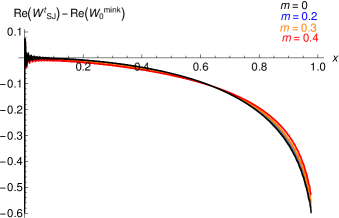
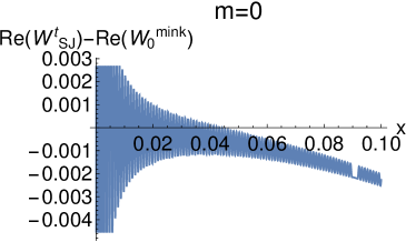
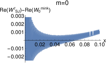
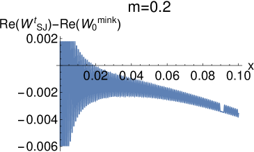
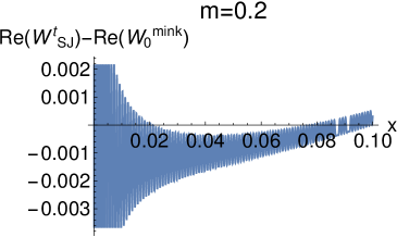
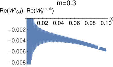
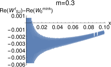
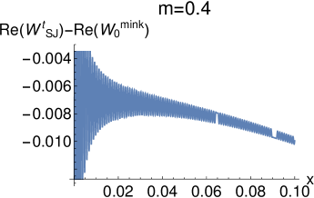
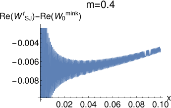
Figure 7: Residue plot of ${\mathrm{Re}}(W_{SJ}^{t}-W^{\mathrm{mink}}_{0})$ for timelike and spacelike separated points respectively, for the full diamond, as well as in a center region of size $l\sim 0.1$.

On the other hand, as we see in Figs. 8 we find that $W_{SJ}^{t}$ clearly does not agree with the massive Minkowski vacuum, in this small mass limit.

         

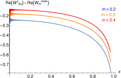
Figure 8: Residue plot of ${\mathrm{Re}}(W_{SJ}^{t}-W^{\mathrm{mink}}_{m})$ for timelike and spacelike separated points respectively, for the full diamond. The discrepancy is obvious.

A similar calculation in the corner shows that $W_{SJ}^{t}$ looks like the massive mirror vacuum rather than the Rindler vacuum. Here, we consider pairs of points: $(u,v)=(l+x,-l+x)$ and $(u^{\prime},v^{\prime})=(l-x,-l-x)$ for timelike separation and $(u,v)=(l+x,-l-x)$ and $(u^{\prime},v^{\prime})=(l-x,-l+x)$ for spacelike separation, where the origin $(0,0)$ is at the left corner of the diamond $\mathcal{D}$ and $2l$ is the length of the corner diamond $\mathcal{D}_{c}$. This is shown in the residue plots in Figs. 9 and 10.

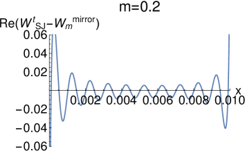
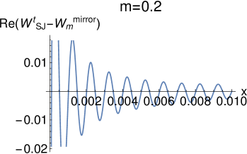
Figure 9: Residue plot of ${\mathrm{Re}}(W_{SJ}^{t}-W^{\mathrm{mink}}_{m})$ for timelike and spacelike separated points respectively in the corner region, $l\sim 0.01$.

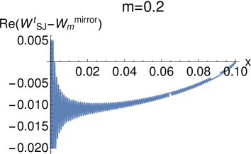
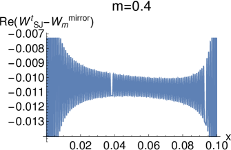
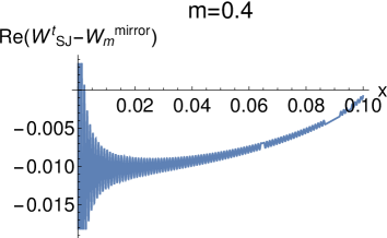
Figure 10: Residue plot of ${\mathrm{Re}}(W_{SJ}^{t}-W^{\mathrm{mink}}_{m})$ for timelike and spacelike separated points respectively in the corner region, $l\sim 0.1$.

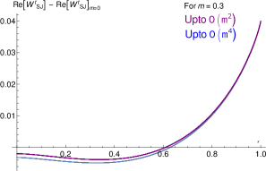
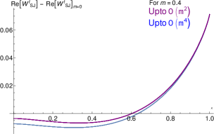
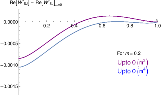
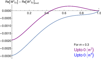
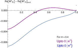
Figure 11: Plot of ${\mathrm{Re}}(W_{SJ}^{t})-{\mathrm{Re}}(W_{SJ})_{m=0}$ vs x for $\mathcal{O}(m^{2})$ and $\mathcal{O}(m^{4})$ corrections. The plots in the first line are all for timelike separated points while those in the second line are for spacelike separated points.

Our calculation suggest that the $\mathcal{O}(m^{4})$ corrections are largely irrelevant to $W_{SJ}$ in the center and the corner of $\mathcal{D}$. A question that occurs is whether increasing the order of the correction makes a significant difference. In Fig. 11 we show the sensitivity of the difference in $W_{SJ}^{t}$ with $W^{\mathrm{mink}}_{0}$, to $\mathcal{O}(m^{2})$ and $\mathcal{O}(m^{4})$. As we can see, the $\mathcal{O}(m^{4})$ corrections while not negligible, are relatively small for $m\sim 0.2$.

What we have seen from our calculations so far is that in the small mass approximation, $W_{SJ}$ continues to behave in the center like the massless Minkowski vacuum, and in the corner as the massive Mirror vacuum. This behavior is very curious since it suggests an unexpected mass dependence in $W_{SJ}$, not seen in the standard vacuum. In order to explore this we must examine $W_{SJ}$ for large masses. Because we are limited in our analytic calculations, we now proceed to a fully numerical calculation of $W_{SJ}$ in a causal set for comparison.

5 The massive SJ Wightman function in the causal set

This curious behavior of the SJ vacuum seems to be a result of our small mass approximation. Since we do not know how to evaluate it analytically for finite mass we look for a numerical evaluation on a causal set ${\cal C}_{\cal M}$ that is approximated by $\mathcal{D}$ (see [16, 17] for an introduction to causal sets).

${\cal C}_{\cal M}$ is obtained via a Poisson sprinkling into $\mathcal{D}$ at density $\rho$. The expected total number of elements is then $\langle N\rangle=\rho V_{\cal M}$, where $V_{\cal M}$ is the total volume of the spacetime manifold in which the elements are sprinkled. The partial order is then determined by the causal relation among the elements i.e. $X_{i}\prec X_{j}$ iff $X_{j}$ is in the causal future of $X_{i}$.

The causal set SJ Wightman function $W^{c}_{SJ}$ is constructed using the same procedure as in the continuum, namely starting from the causal set retarded Green function. The massive Green function in $\mathcal{D}$ is [4, 18]

$$G_{m}=\left({\mathbb{I}}+\frac{m^{2}}{\rho}G_{0}\right)^{-1}G_{0},$$ (132)

where ${\mathbb{I}}$ is the $N\times N$ identity matrix and $G_{0}$ is the massless retarded Green function. Defining the causal matrix $C$ on ${\cal C}_{\cal M}$ as $C_{ij}=1$ if $X_{i}\prec X_{j}$ and $C_{ij}=0$ otherwise, we see that $G_{0}=C/2$.

We sprinkle $N=10,000$ elements in $\mathcal{D}$ of length $2$, i.e., of density $\rho=2500$ for $m=0.2,0.4,0.6,0.8,1,2$ and $10$. In Fig. 12 we plot the SJ eigenvalues for these various masses. We find that the eigenvalues for small masses are very close to the massless eigenvalues, especially for small $n$. As $n$ increases, they become indistinguishable. In Fig. 13 we show the scatter plot of $W^{c}_{SJ}$. For the smaller masses, $W^{c}_{SJ}$ tracks the massless case closely, but at larger masses $m\sim 10$ it shows the characteristic behavior expected of the massive Minkowski vacuum [2].

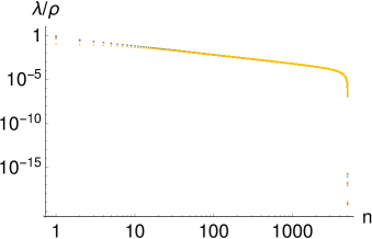
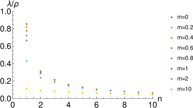
(a)	(b)

Figure 12: (a):A log-log plot of the SJ eigenvalues $\lambda$ divided by density $\rho$ vs $n$ for $m=0,0.2,0.4,0.6,0.8,1,2$ and $10$, (b): a plot of $\lambda/\rho$ vs $n$ for small $n$.

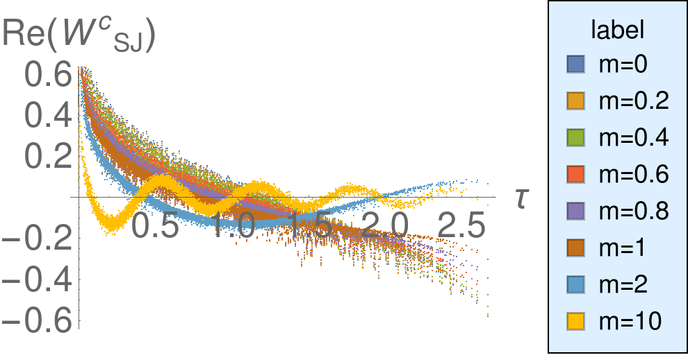
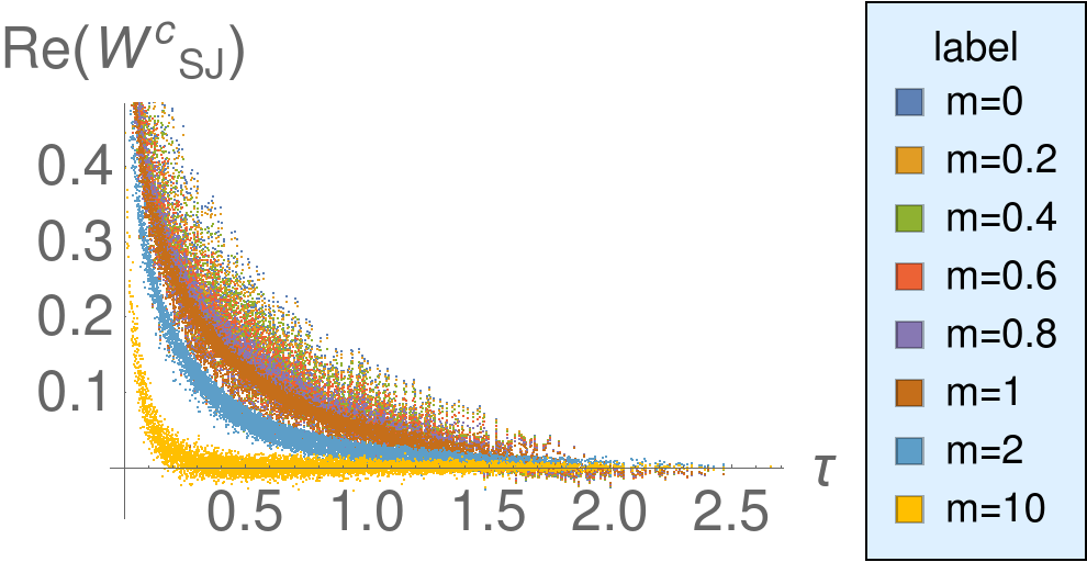
(a)	(b)

Figure 13: $W^{c}_{SJ}$ for $m=0,0.2,0.4,0.6,0.8,1,2$ and $10$ for timelike and spacelike separated points.

Next, we focus our attention to the center of the diamond so that we can compare with our analytic results. We consider a central region $\mathcal{D}_{l}$ with $l=0.1$. Figs  14 and  15 shows $W^{c}_{SJ}$ vs proper time and proper distance for timelike and spacelike separated pairs, respectively for small and large masses. The comparisons with the massless and massive Minkowski vacuum show a curious behavior. For the small $m$ values $W^{c}_{SJ}$ agrees perfectly with our analytic results above, namely that $W_{SJ}$ is more like $W^{\mathrm{mink}}_{0}$ than $W^{\mathrm{mink}}_{m}$. However, as $m$ increases, $W^{\mathrm{mink}}_{m}$ approaches $W^{\mathrm{mink}}_{0}$, coinciding with it at $m=2\Lambda$. After this value of $m$, $W^{c}_{SJ}$ then tracks $W^{\mathrm{mink}}_{m}$ rather than $W^{\mathrm{mink}}_{0}$. This transition is continuous, and suggests that the small $m$ behavior of $W^{c}_{SJ}$ goes continuously over to $W^{\mathrm{mink}}_{0}$, unlike $W^{\mathrm{mink}}_{m}$.

Next we compare $W^{c}_{SJ}$ in the corner of the diamond with $W^{\mathrm{mirror}}_{m}$ and $W^{\mathrm{rind}}_{m}$ for all pair of spacetime points in the left corner of the diamond for a range of masses. Instead of plotting the actual functions, we consider the correlation plot as was done in [3]. To generate these plots we considered a small causal diamond in the corner of length $l=0.2$ which contained 118 elements. $W^{\mathrm{mirror}}_{m}$ and $W^{\mathrm{rind}}_{m}$ were calculated for each pair of elements and compared with $W^{c}_{SJ}$ (see Figs. 16 and 17). In [3] the IR cut-off $\Lambda$ was determined from Fig. 17 for $m=0$ by setting the intercept to zero. We observe that there is much better correlation between $W_{SJ}$ and $W^{\mathrm{mirror}}_{m}$ as compared to $W^{\mathrm{rind}}_{0}$ for all masses which is in agreement with our analytic calculations.

6 Discussion

In this work, we calculated the massive scalar field SJ modes up to fourth order of mass. The procedure we have developed for solving the central eigenvalue problem can be used in principle to find the SJ modes for higher order mass corrections.

Our work shows that $W^{c}_{SJ}$ in the causal set is compatible with our analytic results in the small mass regime. The curious behavior of $W^{c}_{SJ}$ with mass in the center of the diamond suggests a hidden subtlety in the finite region, ab-initio construction, that has hitherto been missed. In particular, it shows that the massive $W_{SJ}$ in 2D has a well defined massless limit, unlike $W^{\mathrm{mink}}_{m}$. Such a continuous behavior with mass was also seen in the calculation of $W^{c}_{SJ}$ in de Sitter spacetime [7]. A possible source for this behavior is that $W_{SJ}$ is built from the advanced/retarded Green functions, which themselves have a well defined massless limit. It is surprising however that $W_{SJ}$ for small mass lies in the massless representation of the Poincare algebra rather than the expected massive representation. What this means for the uniqueness of the SJ vacuum is unclear and we hope to explore this in future work.

In the corner of the diamond, we see that as in the massless case, $W_{SJ}$ resembles the massive mirror vacuum for all masses. Thus, the expectation (see [3]) that the massive $W_{SJ}$ must be the Rindler vacuum seems to be incorrect.

We end with a broad comment on the SJ formalism. It is possible to construct a $W_{SJ}$ using a different inner product on $\mathcal{F}(M,g)$, instead of the $\mathcal{L}^{2}$ inner product adopted in this work. One way of doing this is to introduce a non trivial weight function in the integral. Thus, different choices of inner product give different SJ Wightman functions even with the same defining conditions (Eqn. (2)). As an almost trivial example, in Appendix  D we show that the choice of inner product can yield the Rindler vacuum in the corner. In future work we hope to explore this possibility in more detail.

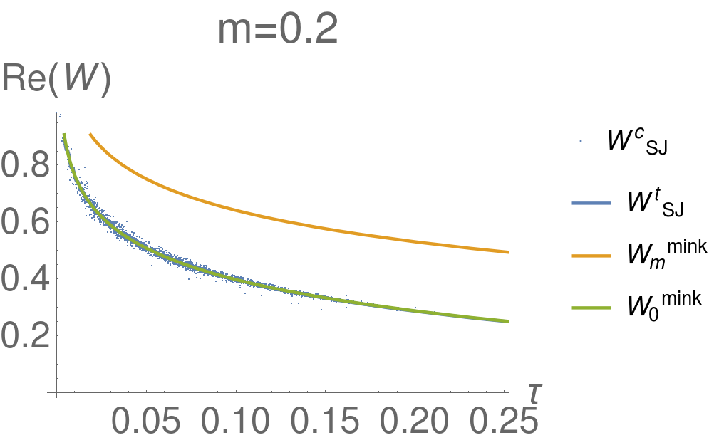
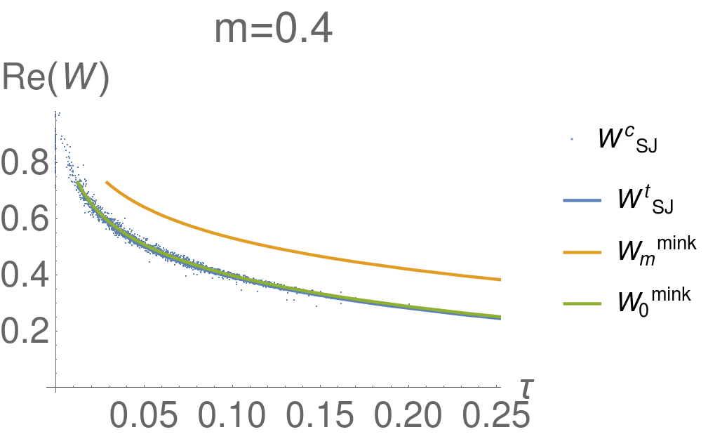
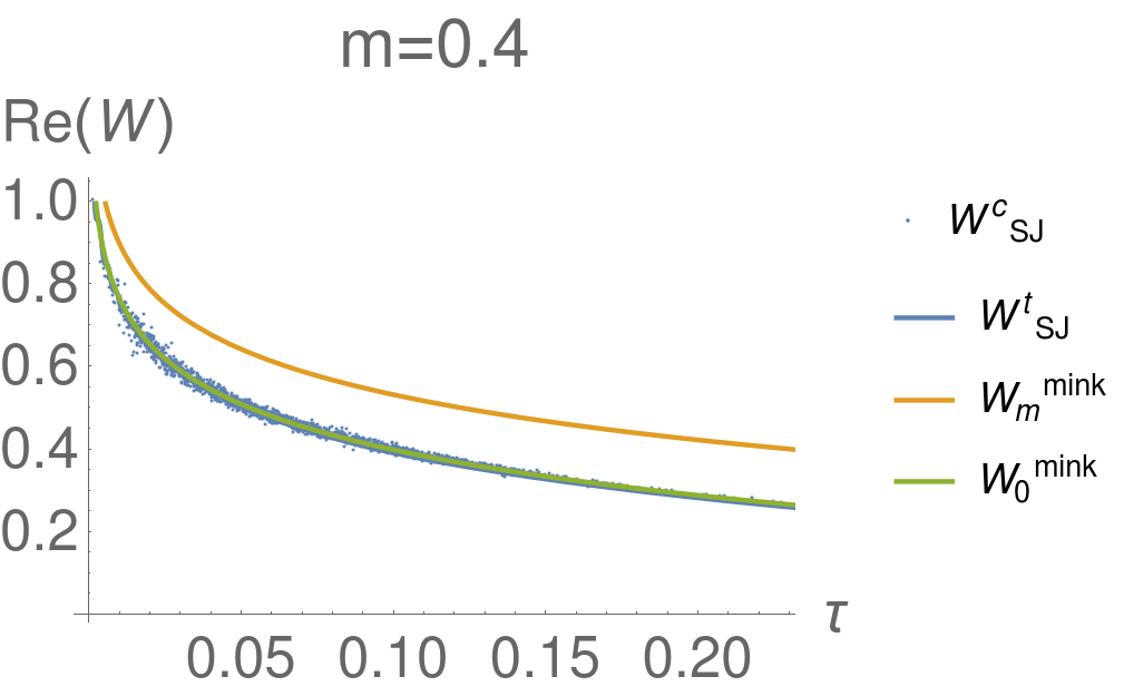
Figure 14: $W^{c}_{SJ}$ (blue dots) vs proper time ($\tau$) in the center of the diamond. The plots on the left are for timelike separated points and those on the right are for spacelike separated points, for the small mass regime, $m=0.2$ and $0.4$. We show $W^{\mathrm{mink}}_{0}$ (green), $W^{\mathrm{mink}}_{m}$ (orange) and our previous analytic calculation of $W_{SJ}$ (blue line). The scatter plot clearly follows the massless green curve for these masses.

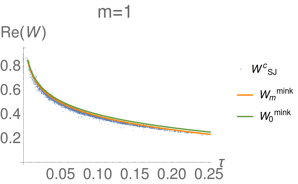
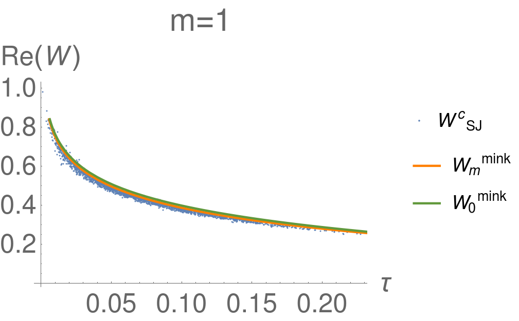
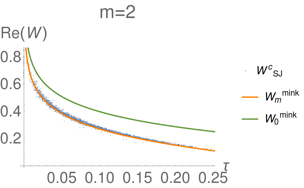
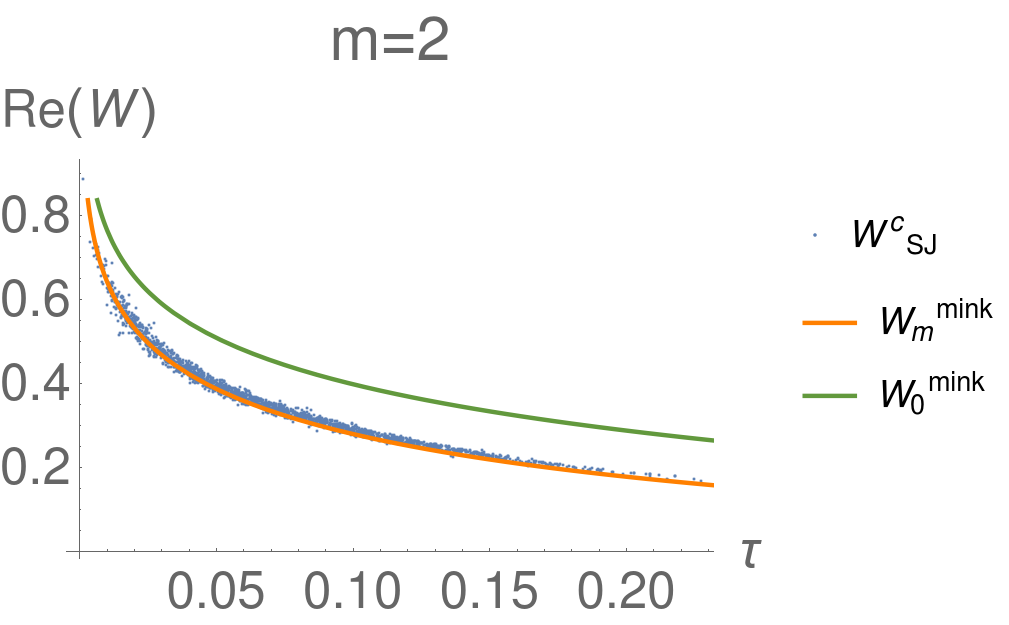
Figure 15: The same plots as in Fig 14 but for $m=1$ and $m=2$. The scatter plot follows the massive orange curve for $m\geq m_{c}$.

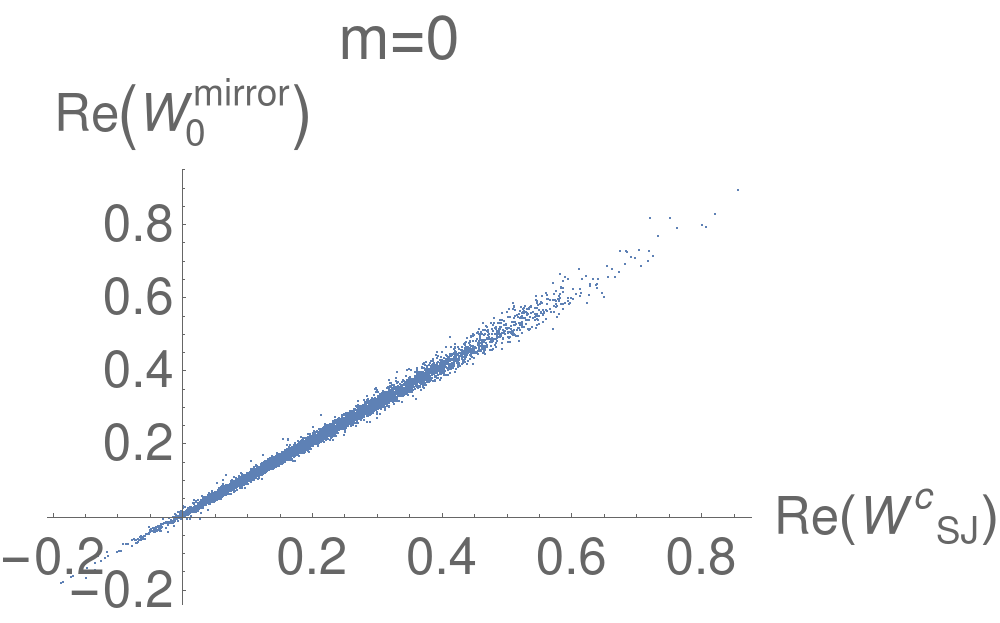
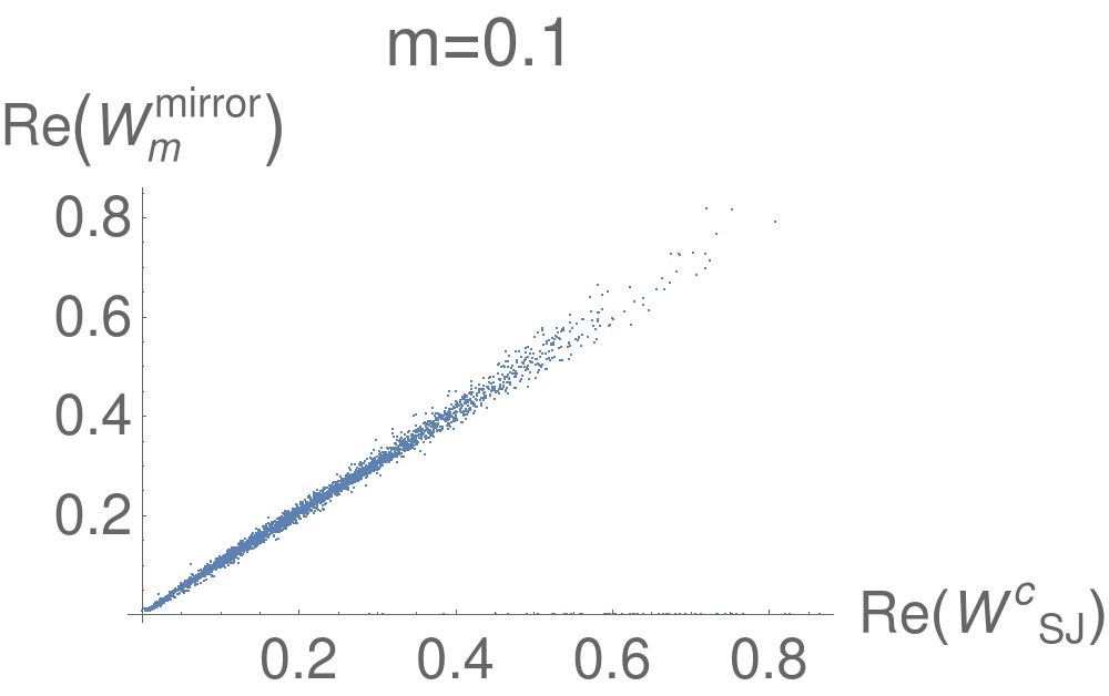
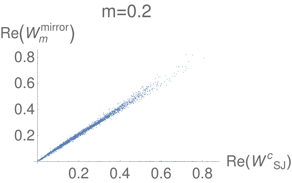
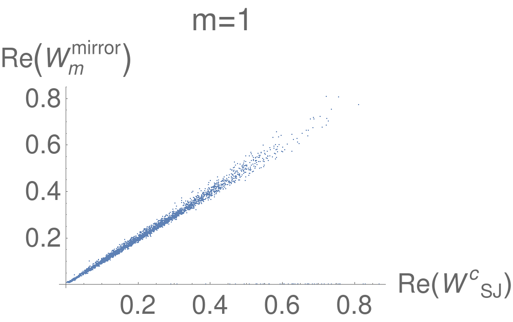
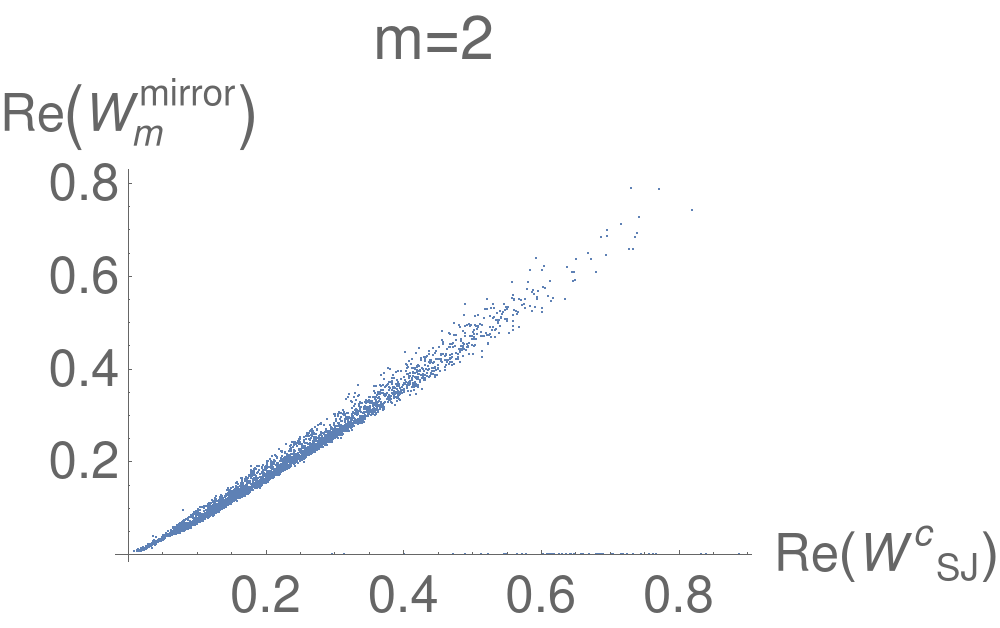
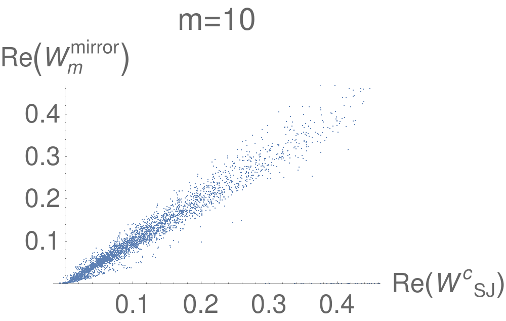
Figure 16: Correlation plot of $W^{c}_{SJ}$ vs $W^{\mathrm{mirror}}_{m}$ in the left corner of the diamond for a range of masses.

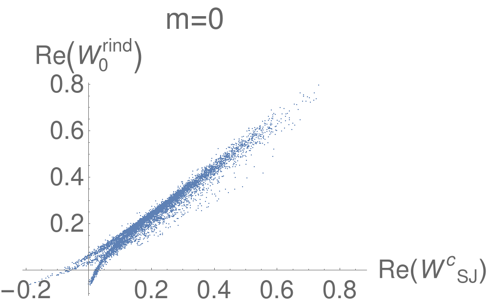
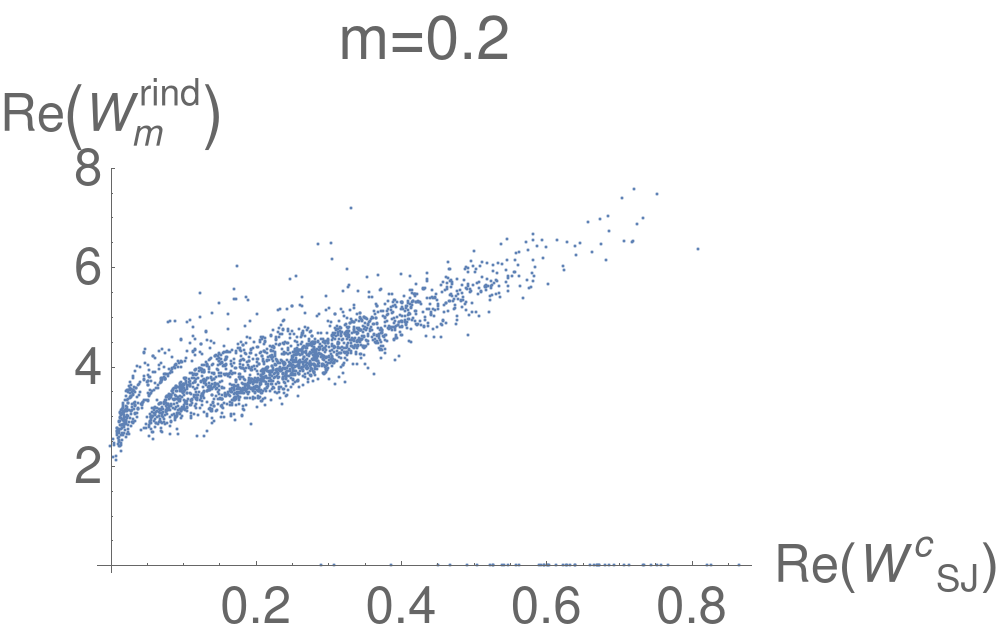
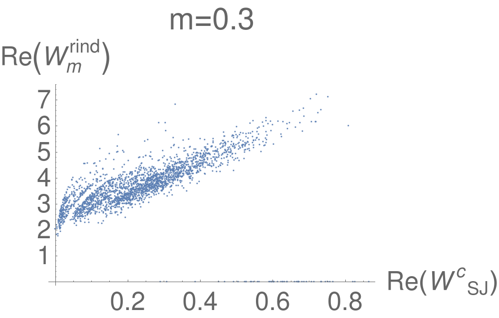
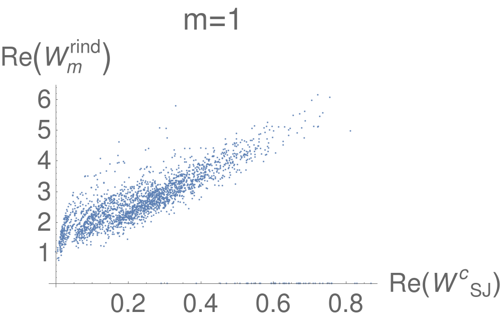
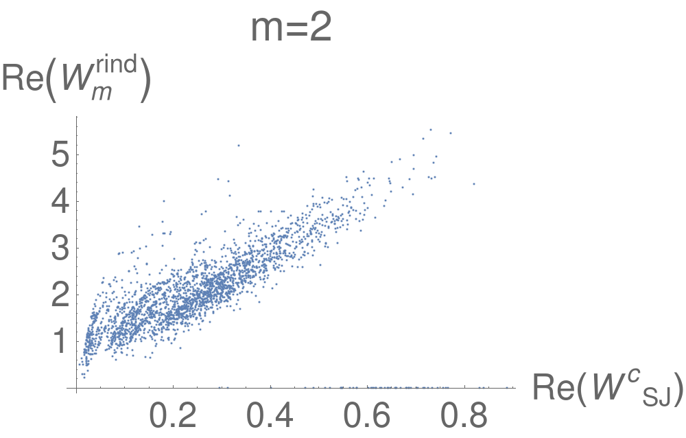
Figure 17: Correlation plot of $W^{c}_{SJ}$ vs $W^{\mathrm{rind}}_{m}$ in the left corner of the diamond for a range of masses.

7 Acknowledgement

We would like to thank Nomaan X, Rafael D. Sorkin, Yasaman K. Yazdi, Sujit K. Nath, and Joseph Samuel for helpful discussions. We would also like to thank S. Vaidya for help with references. During this work S.S. was supported in part by FQXi-MGA-1510 of the Foundational Questions Institute and an Emmy Noether Fellowship at the Perimeter Institute for Theoretical Physics. S.S. is currently partly supported by a Visiting Fellowship at the Perimeter Institute for Theoretical Physics.

Appendix A Some expressions and derivation of results used in Sec. 3

In this appendix we add some of the details of the calculations of Sec. 3. These details include the simplified expression of $F_{ik,n}(u,v)$ and $G_{ik,n}(u,v)$ for $n=0,1,2$ , $Z^{A/S}_{l}(u,v)$ and $i\hat{\Delta}\circ Z^{A/S}_{l}(u,v)$, for $l=0,1,2$ and $P^{A/S}_{n}(u,v)$ for $n=0,1,2$ up to the order in $m^{2}$, which is required in the calculation of SJ modes up to $\mathcal{O}(m^{4})$. Some details of the calculations of $u^{A}_{k}(u,v)$ and $u^{S}_{k}(u,v)$ can be found in Appendix A.1 and A.2 respectively.

Evaluating $F_{ik,n}(u,v)$ and $G_{ik,n}(u,v)$ defined in Eqn. (51) for $n=0,1,2$, we get

$$F_{ik,0}(u,v) = v,$$

$$F_{ik,1}(u,v) = \frac{iv^{2}}{2k}-\frac{1}{4}(v^{2}u+2v+u),$$

$$F_{ik,2}(u,v) = -\frac{v^{3}}{8k^{2}}-\frac{i}{24k}(2v^{3}u+3v^{2}-1)+\frac{1}{48}(v^{3}u^{2}+v^{3}+6v^{2}u+3vu^{2}+3v+2u).$$

$$G_{ik,0}(u,v) = -1,$$

$$G_{ik,1}(u,v) = -\frac{iv}{2k}+\frac{1}{4}(v^{2}+2uv+1),$$

$$G_{ik,2}(u,v) = \frac{v^{2}}{8k^{2}}+\frac{i}{24k}(2v^{3}+3uv^{2}-u)-\frac{1}{48}(2v^{3}u+3v^{2}u^{2}+3v^{2}+6uv+u^{2}+1).$$

Next, we list $Z^{A}_{l}(u,v)$ and $Z^{S}_{l}(u,v)$ defined in Eqn. (16) and Eqn. (25) for $l=0,1,2$ up to the required order of $m^{2}$.

$$Z^{A}_{0}(u,v)=0, Z^{S}_{0}(u,v)\approx 2-m^{2}uv+\frac{m^{4}}{8}u^{2}v^{2},$$

$$Z^{A}_{1}(u,v)\approx(u-v)-\frac{m^{2}}{4}uv(u-v), Z_{1}^{S}(u,v)\approx(u+v)-\frac{m^{2}}{4}uv(u+v),$$

$$Z^{A}_{2}(u,v)\approx u^{2}-v^{2}, Z^{S}_{2}(u,v)\approx u^{2}+v^{2}.$$ (133)

Next, we list $i\hat{\Delta}\circ Z^{A}_{l}(u,v)$ and $i\hat{\Delta}\circ Z^{S}_{l}(u,v)$ for $l=0,1,2$ up to the required order of $m^{2}$, where $i\hat{\Delta}\circ Z_{l}(u,v)$ is described in Eqn. (44)

$$i\hat{\Delta}\circ Z^{A}_{0}(u,v) = 0,$$

$$i\hat{\Delta}\circ Z^{S}_{0}(u,v) \approx -i\frac{L^{2}}{24}(u+v)(48-12m^{2}(1+uv)+m^{4}(3+3uv+u^{2}v^{2}))),$$

$$i\hat{\Delta}\circ Z^{A}_{1}(u,v) \approx iL^{2}\left(-\frac{1}{2}(u^{2}-v^{2})+\frac{m^{2}}{24}(2uv+1)(u^{2}-v^{2})\right),$$

$$i\hat{\Delta}\circ Z^{S}_{1}(u,v) \approx iL^{2}\left(\frac{1}{2}(2-u^{2}-v^{2})-\frac{m^{2}}{24}\left(6(1+2uv)+(u^{2}+v^{2})(1-2uv)\right)\right),$$

$$i\hat{\Delta}\circ Z^{A}_{2}(u,v) \approx \frac{iL^{2}}{3}\left((u-v)-(u^{3}-v^{3})\right),$$

$$i\hat{\Delta}\circ Z^{S}_{2}(u,v) \approx \frac{iL^{2}}{3}\left((u+v)-(u^{3}+v^{3})\right).$$ (134)

$P^{A/S}_{n}(u,v)$ defined in Eqn. (58) for $n=0,1,2$.

$$P_{0}^{A}(u,v) = 0,$$

$$P_{1}^{A}(u,v) = \left(i\left(\frac{1}{2k}-Q^{A}_{1}(k)\right)(u-v)-\frac{1}{4}(u^{2}-v^{2})\right),$$

$$P_{2}^{A}(u,v) = -\frac{u^{2}-v^{2}}{8k^{2}}-\frac{i}{24k}(u-v)(2u^{2}+2v^{2}+5uv+1)+\frac{1}{24}(1+uv)(u^{2}-v^{2}),$$ (135)

$$+Q^{A}_{1}(k)\left(\frac{u^{2}-v^{2}}{2k}+\frac{i}{4}(u-v)(uv+1)\right)-iQ^{A}_{2}(k)(u-v),$$

$$P_{0}^{S}(u,v) = \frac{}{}-2+2ik(u+v),$$

$$P_{1}^{S}(u,v) = -\frac{i(u+v)}{2k}+\frac{1}{4}(u^{2}+v^{2}+4uv+2)-\left(u^{2}+v^{2}+\frac{ik}{2}(uv+3)(u+v)\right)+iQ_{1}^{S}(k)(u+v),$$

$$P_{2}^{S}(u,v) = \frac{u^{2}+v^{2}}{8k^{2}}+\frac{i}{24k}(u+v)(2u^{2}+2v^{2}+uv-1)-\frac{1}{48}((2uv+4)(u^{2}+v^{2})+6v^{2}u^{2}+12uv+2)$$ (136)

$$+2k\left(-\frac{i(u^{3}+v^{3})}{8k^{2}}+\frac{1}{24k}((2uv+3)(u^{2}+v^{2})-2)+\frac{i}{48}(u+v)(u^{2}v^{2}+u^{2}+v^{2}+8uv+5)\right)$$

$$+Q_{1}^{S}(k)\left(-\frac{u^{2}+v^{2}}{2k}-\frac{i}{4}(uv+3)(u+v)\right)+iQ_{2}^{S}(k)(u+v),$$

where $Q^{A}_{n}(k)$ and $Q^{S}_{n}(k)$ for $n=1,2$ can be found in Sec. A.1 and A.2 respectively.

A.1 Details of the calculations for the antisymmetric SJ modes

In this section we solve Eqn. (57) for $H^{A}_{k}(u,v)$ by constructing each $m^{2n}P^{A}_{n}(u,v)$ out of $Z_{l}(u,v)$ and $i\Delta\circ Z_{l}(u,v)$ for different $l$. Let us start with the first non zero $P^{A}_{n}(u,v)$. It can be observed that $m^{2}P^{A}_{1}(u,v)$ can be constructed out of $m^{2}Z^{A}_{1}(u,v)$ and $m^{2}i\Delta\circ Z^{A}_{1}(u,v)$ up to $\mathcal{O}(m^{2})$ as

$$m^{2}P^{A}_{1}(u,v)=\frac{im^{2}}{2L^{2}}\left(\frac{L^{2}}{k}\left(1-2kQ^{A}_{1}(k)\right)Z^{A}_{1}(u,v)-i\Delta\circ Z^{A}_{1}(u,v)\right)$$ (137)

To make the term in the bracket look like $\left(i\Delta+\frac{L^{2}}{k}\right)\circ Z^{A}_{1}(u,v)$, we fix

$$Q^{A}_{1}(k)=\frac{1}{k}.$$ (138)

Therefore Eqn. (57) for $H^{A}_{k}(u,v)$ up to $\mathcal{O}(m^{4})$ can be written as

$$\left(i\Delta+\frac{L^{2}}{k}\right)\circ\left(H^{A}_{k}(u,v)+\frac{im^{2}\cos(k)}{2k}Z^{A}_{1}(u,v)\right)-\frac{m^{4}L^{2}\cos(k)}{k}\left(\frac{3(u^{2}-v^{2})}{8k^{2}}-\frac{i}{12k}(u^{3}-v^{3})\right.$$

$$\quad\left.+\frac{5i}{24k}(u-v)+\frac{1}{48}(u^{2}-v^{2})-iQ^{A}_{2}(k)(u-v)\right)=0.$$

(139)

In the remaining terms, i.e., the terms which are not yet written as $Z^{A}_{l}(u,v)$ or $i\Delta\circ Z^{A}_{l}(u,v)$, the highest order of $u$ and $v$ are $u^{3}$ and $v^{3}$, which can be identified with $i\Delta\circ Z_{2}(u,v)$. Therefore we use

$$-\left(i\Delta+\frac{L^{2}}{k}\right)\circ\frac{m^{4}\cos(k)}{4k^{2}}Z^{A}_{2}(u,v)=-\frac{m^{4}L^{2}\cos(k)}{k}\left(\frac{i}{12k}(u-v)-\frac{i}{12k}(u^{3}-v^{3})+\frac{1}{4k^{2}}(u^{2}-v^{2})\right),$$ (140)

to write Eqn. (139) as

$$\left(i\Delta+\frac{L^{2}}{k}\right)\circ\left(H^{A}_{k}(u,v)+\cos(k)\left(\frac{im^{2}}{2k}Z^{A}_{1}(u,v)-\frac{m^{4}}{4k^{2}}Z^{A}_{2}(u,v)\right)\right)$$

$$-\frac{m^{4}L^{2}\cos(k)}{k}\left(\frac{u^{2}-v^{2}}{8k^{2}}+\frac{i}{8k}(u-v)+\frac{1}{48}(u^{2}-v^{2})-iQ^{A}_{2}(k)(u-v)\right)=0.$$ (141)

The remaining terms in Eqn. (141) can be written as

$$\left(i\Delta+\frac{L^{2}}{k}\right)\circ\left(-\frac{im^{4}\cos(k)}{24k^{3}}(6+k^{2})Z^{A}_{1}(u,v)\right),$$ (142)

by fixing

$$Q^{A}_{2}(k)=\frac{1}{12k}-\frac{1}{4k^{3}}.$$ (143)

Finally Eqn. (141) can be written as

$$\left(i\Delta+\frac{L^{2}}{k}\right)\circ\left(H^{A}_{k}(u,v)+\cos(k)\left(\left(\frac{im^{2}}{2k}-\frac{im^{4}(6+k^{2})}{24k^{3}}\right)Z^{A}_{1}(u,v)-\frac{m^{4}}{4k^{2}}Z^{A}_{2}(u,v)\right)\right)=0$$ (144)

which implies that

$$u^{A}_{k}(u,v)=U^{A}_{ik}(u,v)-\cos(k)\left(\left(\frac{im^{2}}{2k}-\frac{im^{4}(6+k^{2})}{24k^{3}}\right)Z^{A}_{1}(u,v)-\frac{m^{4}}{4k^{2}}Z^{A}_{2}(u,v)\right)+\mathcal{O}(m^{6})$$ (145)

with eigenvalue $-\frac{L^{2}}{k}$, where $k$ satisfies

$$\sin(k)=\left(\frac{m^{2}}{k}+\frac{m^{4}}{12k}\left(1-\frac{3}{k^{2}}\right)\right)\cos(k)+\mathcal{O}(m^{6})$$ (146)

A.2 Details of the calculations for the symmetric SJ modes

In this section we solve Eqn. (57) for $H^{S}_{k}(u,v)$ by constructing each $m^{2n}P^{S}_{n}(u,v)$ out of $Z_{l}(u,v)$ and $i\Delta\circ Z_{l}(u,v)$ for different $l$. Let us start with the first non zero $P^{S}_{n}(u,v)$. It can be observed that $P^{S}_{0}(u,v)$ can be constructed out of $Z^{S}_{0}(u,v)$ and $i\Delta\circ Z^{S}_{0}(u,v)$ up to $\mathcal{O}(m^{0})$ as

$$P^{S}_{0}(u,v)=\left(i\Delta+\frac{L^{2}}{k}\right)\circ\left(-\frac{k}{L^{2}}Z^{S}_{0}(u,v)\right).$$ (147)

Therefore Eqn. (57) for $H^{S}_{k}(u,v)$ up to $\mathcal{O}(m^{4})$ can be written as

$$\left(i\Delta+\frac{L^{2}}{k}\right)\circ\left(H^{S}_{k}(u,v)+Z^{S}_{0}(u,v)\cos(k)\right)-\frac{L^{2}\cos(k)}{k}\left(m^{2}\left(-\frac{3}{4}(u^{2}+v^{2})\right.\right.$$

$$\left.\left.+i\left(Q^{S}_{1}(k)-k-\frac{1}{2k}\right)(u+v)+\frac{1}{2}\right)+m^{4}\left(\frac{u^{2}+v^{2}}{8k^{2}}+\frac{i}{24k}(u+v)(2u^{2}+2v^{2}+uv-1)\right.\right.$$

$$\left.\left.-\frac{1}{24}((-3uv-4)(u^{2}+v^{2})+6uv+5)+\left(-\frac{i(u^{3}+v^{3})}{4k}+\frac{ik}{24}(u+v)(u^{2}+v^{2}+5uv+2)\right)\right.\right.$$

$$\left.\left.+Q^{S}_{1}(k)\left(-\frac{u^{2}+v^{2}}{2k}-\frac{i}{4}(uv+3)(u+v)\right)+iQ^{S}_{2}(k)(u+v)\right)\right)=0.$$ (148)

Since the extra terms in Eqn. (148) has $m^{2}$ as a factor, we need to look for $Z^{S}_{l}$ and $i\Delta\circ Z^{S}_{l}$ only up to $\mathcal{O}(m^{2})$. $\mathcal{O}(m^{2})$ terms in Eqn. (148) can be written in terms of $\left(i\Delta+\frac{L^{2}}{k}\right)\circ Z^{S}_{0}(u,v)$ and $\left(i\Delta+\frac{L^{2}}{k}\right)\circ Z^{S}_{1}(u,v)$ for

$$Q^{S}_{1}=2k-\frac{1}{k}$$ (149)

as

$$\left(i\Delta+\frac{L^{2}}{k}\right)\circ m^{2}\cos(k)\left(\frac{3i}{2k}Z^{S}_{1}(u,v)+\frac{1}{2}Z^{S}_{0}(u,v)\right).$$ (150)

Therefore Eqn. (148) can further be written as

$$\left(i\Delta+\frac{L^{2}}{k}\right)\circ\left(H^{S}_{k}(u,v)+\cos(k)\left(\left(1+\frac{m^{2}}{2}\right)Z^{S}_{0}(u,v)+\frac{3im^{2}}{2k}Z^{S}_{1}(u,v)\right)\right)+\frac{im^{4}L^{2}\cos(k)}{48k^{3}}\left(8ik^{2}\right.$$

$$\left.+k\left(-34-kQ^{S}_{2}(k)+56k^{2}\right)(u+v)+i(30-37k^{2})(u^{2}+v^{2})+2k(4-k^{2})(u^{3}+v^{3})\right)=0.$$ (151)

Remaining $\mathcal{O}(m^{4})$ terms in Eqn. (151) can be written in terms of $\left(i\Delta+\frac{L^{2}}{k}\right)\circ Z^{S}_{0}(u,v)$, $\left(i\Delta+\frac{L^{2}}{k}\right)\circ Z^{S}_{1}(u,v)$, $\left(i\Delta+\frac{L^{2}}{k}\right)\circ Z^{S}_{2}(u,v)$ for

$$Q^{S}_{2}(k)=\frac{3-29k^{2}+28k^{4}}{12k^{3}}$$ (152)

as

$$-\frac{m^{4}\cos(k)}{8k^{2}}\left((4-k^{2})Z^{S}_{2}(u,v)+\frac{i(6-31k^{2})}{3k}Z^{S}_{1}(u,v)+(2-9k^{2})Z^{S}_{0}(u,v)\right).$$ (153)

Hence Eqn. (151) can be written as

$$\left(i\Delta+\frac{L^{2}}{k}\right)\circ\left(H^{S}_{k}(u,v)+\cos(k)\left(\left(1+\frac{m^{2}}{2}-\frac{m^{4}}{8k^{2}}(2-9k^{2})\right)Z^{S}_{0}(u,v)\right.\right.$$

$$\left.\left.+\left(\frac{3im^{2}}{2k}-\frac{im^{4}}{24k^{3}}(6-31k^{2})\right)Z^{S}_{1}(u,v)-\frac{m^{4}}{8k^{2}}(4-k^{2})Z^{S}_{2}(u,v)\right)\right)=0.$$ (154)

Therefore the symmetric SJ modes are

$$u^{S}_{k}(u,v) = U^{S}_{ik}(u,v)-\cos(k)\left(\left(1+\frac{m^{2}}{2}-\frac{m^{4}}{8k^{2}}(2-9k^{2})\right)Z^{S}_{0}(u,v)\right.$$ (155)

$$\left.+\left(\frac{3im^{2}}{2k}-\frac{im^{4}}{24k^{3}}(6-31k^{2})\right)Z^{S}_{1}(u,v)-\frac{m^{4}}{8k^{2}}(4-k^{2})Z^{S}_{2}(u,v)\right)+\mathcal{O}(m^{4}),$$

with eigenvalue $-\frac{L^{2}}{k}$, where $k$ satisfies

$$\sin(k)=\left(2k-\frac{m^{2}}{k}(1-2k^{2})+\frac{m^{4}}{12k^{3}}(3-29k^{2}+28k^{4})\right)\cos(k)+\mathcal{O}(m^{4}).$$ (156)

Appendix B Summation of series with inverse powers of roots of a transcendental equation

In this appendix we make use of the work of [13] to evaluate the series (Eqn. (79) and Eqn. (80)), which involves the roots of the transcendental equation (Eqn. (43)). They are used in Sec(3.2) to determine the completeness of the SJ modes

Let us start with a brief discussion on the work of [13]. Consider a transcendental equation of the form

$$S(x)\equiv 1+\sum_{n=1}^{\infty}a_{n}x^{n}=0$$ (157)

with $x_{1},x_{2},x_{3}\dots$ as its roots, which means the equation can be factorized as

$$\left(1-\frac{x}{x_{1}}\right)\left(1-\frac{x}{x_{2}}\right)\left(1-\frac{x}{x_{3}}\right)\dots=0$$ (158)

On comparing Eqn. (157 and 158), we find that

$$a_{1}=\sum_{i=1}^{\infty}\frac{1}{x_{i}},\quad a_{2}=\sum_{i<j}\frac{1}{x_{i}x_{j}},\quad a_{3}=\sum_{i<j<k}\frac{1}{x_{i}x_{j}x_{k}}$$ (159)

and so on. It is straight forward to see that

$$\sum_{i=1}^{\infty}\left(\frac{1}{x_{i}}\right)^{2}=\left(\sum_{i=1}^{\infty}\frac{1}{x_{i}}\right)^{2}-2\sum_{i<j}\frac{1}{x_{i}x_{j}}=a_{1}^{2}-2a_{2}$$ (160)

and similarly

$$\sum_{i=1}^{\infty}\left(\frac{1}{x_{i}}\right)^{3}=3a_{1}a_{2}-3a_{3}-a_{1}^{3}.$$ (161)

Similarly we can get the sum of higher inverse powers of the roots.

Now let us come to the equation of our interest i.e. Eqn. (43), which on series expansion becomes

$$S(k^{2})\equiv 1-\left(1-\frac{1}{3!}\right)k^{2}+\left(\frac{2}{4!}-\frac{1}{5!}\right)k^{4}-\left(\frac{2}{6!}-\frac{1}{7!}\right)k^{6}\dots=0.$$ (162)

The roots of Eqn. (162) are $k^{S}_{0}\in\mathcal{K}_{g}$, and therefore

$$\sum_{k^{S}_{0}\in\mathcal{K}_{g}}\frac{1}{{k^{S}_{0}}^{2}} = a_{1}=\frac{5}{6},$$

$$\sum_{k^{S}_{0}\in\mathcal{K}_{g}}\frac{1}{{k^{S}_{0}}^{4}} = a_{1}^{2}-2a_{2}=\frac{49}{90},$$

$$\sum_{k^{S}_{0}\in\mathcal{K}_{g}}\frac{1}{{k^{S}_{0}}^{6}} = 3a_{1}a_{2}-3a_{3}-a_{1}^{3}=\frac{377}{945}.$$ (163)

We are also interested in the series involving the inverse power of $4{k^{S}_{0}}^{2}-1$, where $k^{S}_{0}\in\mathcal{K}_{g}$. We start with finding an equation whose solutions are given by $4{k^{S}_{0}}^{2}-1$. If ${k^{S}_{0}}^{2}$ are the solutions of $S(k^{2})=0$, then $4{k^{S}_{0}}^{2}-1$ are the solutions of $S\left(\frac{k^{2}+1}{4}\right)=0$.

$$S\left(\frac{k^{2}+1}{4}\right)\equiv 1-\frac{1}{4}k^{2}+\frac{5\cos(1/2)-9\sin(1/2)}{32\left(\cos(1/2)-\sin(1/2)\right)}k^{4}-\frac{53\cos(1/2)-97\sin(1/2)}{384\left(\cos(1/2)-\sin(1/2)\right)}k^{6}\dots=0.$$ (164)

Using the same method as above, we find

$$\sum_{k^{S}_{0}\in\mathcal{K}_{g}}\frac{1}{4{k^{S}_{0}}^{2}-1} = \frac{1}{4},$$ (165)

$$\sum_{k^{S}_{0}\in\mathcal{K}_{g}}\frac{1}{(4{k^{S}_{0}}^{2}-1)^{2}} = -\frac{1}{4}\left(\frac{\cos(1/2)-2\sin(1/2)}{\cos(1/2)-\sin(1/2)}\right),$$ (166)

$$\sum_{k_{0}\in\mathcal{K}_{g}}\frac{1}{(4{k^{S}_{0}}^{2}-1)^{3}} = \frac{1}{64}\left(1+\frac{19\cos(1/2)-35\sin(1/2)}{\cos(1/2)-\sin(1/2)}\right).$$ (167)

Appendix C Some expressions used in Sec. 4

Here we list the expressions of $A_{\mathrm{I}},A_{\mathrm{II}},A_{\mathrm{III}}$ and $A_{\mathrm{IV}}$ defined in Eqn. (LABEL:eq:aone) in terms of Polylogarithms.

$$A_{\mathrm{I}} \equiv \sum_{n=1}^{\infty}\frac{1}{8n\pi}\left(1-\frac{2m^{2}}{n^{2}\pi^{2}}+\frac{m^{4}}{n^{2}\pi^{2}}\left(\frac{7}{n^{2}\pi^{2}}-\frac{1}{6}\right)\right)\left(e^{-in\pi u}-e^{-in\pi v}\right)\left(e^{in\pi u^{\prime}}-e^{in\pi v^{\prime}}\right)$$ (168)

$$= \frac{1}{8\pi}\left[{\mathrm{Li}}_{1}\left(e^{-i\pi(u-u^{\prime})}\right)+{\mathrm{Li}}_{1}\left(e^{-i\pi(v-v^{\prime})}\right)-{\mathrm{Li}}_{1}\left(e^{-i\pi(u-v^{\prime})}\right)-{\mathrm{Li}}_{1}\left(e^{-i\pi(v-u^{\prime})}\right)\right]$$

$$-\frac{m^{2}}{4\pi^{3}}\left(1+\frac{m^{2}}{12}\right)\left[{\mathrm{Li}}_{3}\left(e^{-i\pi(u-u^{\prime})}\right)+{\mathrm{Li}}_{3}\left(e^{-i\pi(v-v^{\prime})}\right)-{\mathrm{Li}}_{3}\left(e^{-i\pi(u-v^{\prime})}\right)-{\mathrm{Li}}_{3}\left(e^{-i\pi(v-u^{\prime})}\right)\right]$$

$$+\frac{7m^{4}}{8\pi^{5}}\left[{\mathrm{Li}}_{5}\left(e^{-i\pi(u-u^{\prime})}\right)+{\mathrm{Li}}_{5}\left(e^{-i\pi(v-v^{\prime})}\right)-{\mathrm{Li}}_{5}\left(e^{-i\pi(u-v^{\prime})}\right)-{\mathrm{Li}}_{5}\left(e^{-i\pi(v-u^{\prime})}\right)\right],$$

$$A_{\mathrm{II}} \equiv \sum_{n=1}^{\infty}\frac{1}{8n\pi}\left(1-\frac{2m^{2}}{n^{2}\pi^{2}}\right)\left(e^{-in\pi u}-e^{-in\pi v}\right)\Psi_{A}^{*}(n,u^{\prime},v^{\prime})$$ (169)

$$= \frac{1}{8\pi}\sum_{j=1}^{3}f_{j}^{*}(m;u^{\prime},v^{\prime})\left[{\mathrm{Li}}_{j+1}\left(-e^{-i\pi u}\right)-{\mathrm{Li}}_{j+1}\left(-e^{-i\pi v}\right)\right]+\frac{im^{4}}{8\pi^{4}}(u^{\prime}-v^{\prime})\left[{\mathrm{Li}}_{4}\left(-e^{-i\pi u}\right)-{\mathrm{Li}}_{4}\left(-e^{-i\pi v}\right)\right]$$

$$+\frac{1}{8\pi}\sum_{j=1}^{3}\left(g_{j}^{*}(m;u^{\prime},v^{\prime})\left[{\mathrm{Li}}_{j+1}\left(e^{-i\pi(u-u^{\prime})}\right)-{\mathrm{Li}}_{j+1}\left(-e^{-i\pi(v-u^{\prime})}\right)\right]\right.$$

$$\left.\quad\quad\quad-g_{j}^{*}(m;v^{\prime},u^{\prime})\left[{\mathrm{Li}}_{j+1}\left(-e^{-i\pi(u-v^{\prime})}\right)-{\mathrm{Li}}_{j+1}\left(-e^{-i\pi(v-v^{\prime})}\right)\right]\right)$$

$$-\frac{im^{4}}{8\pi^{4}}\left((2u^{\prime}+v^{\prime})\left[{\mathrm{Li}}_{4}\left(-e^{-i\pi(u-u^{\prime})}\right)-{\mathrm{Li}}_{4}\left(-e^{-i\pi(v-u^{\prime})}\right)\right]\right.$$

$$\left.\quad\quad\quad-(2v^{\prime}+u^{\prime})\left[{\mathrm{Li}}_{4}\left(-e^{-i\pi(u-v^{\prime})}\right)-{\mathrm{Li}}_{4}\left(-e^{-i\pi(v-v^{\prime})}\right)\right]\right),$$

$$A_{\mathrm{III}} \equiv \sum_{n=1}^{\infty}\frac{1}{8n\pi}\left(1-\frac{2m^{2}}{n^{2}\pi^{2}}\right)\Psi_{A}(n,u,v)\left(e^{in\pi u^{\prime}}-e^{in\pi v^{\prime}}\right)$$ (170)

$$= \frac{1}{8\pi}\sum_{j=1}^{3}f_{j}(m;u,v)\left[{\mathrm{Li}}_{j+1}\left(-e^{i\pi u^{\prime}}\right)-{\mathrm{Li}}_{j+1}\left(-e^{i\pi v^{\prime}}\right)\right]-\frac{im^{4}}{8\pi^{4}}(u-v)\left[{\mathrm{Li}}_{4}\left(-e^{i\pi u^{\prime}}\right)-{\mathrm{Li}}_{4}\left(-e^{i\pi v^{\prime}}\right)\right]$$

$$+\frac{1}{8\pi}\sum_{j=1}^{3}\left(g_{j}(m;u,v)\left[{\mathrm{Li}}_{j+1}\left(e^{-i\pi(u-u^{\prime})}\right)-{\mathrm{Li}}_{j+1}\left(-e^{-i\pi(v-u^{\prime})}\right)\right]\right.$$

$$\left.\quad\quad\quad-g_{j}(m;v,u)\left[{\mathrm{Li}}_{j+1}\left(-e^{-i\pi(u-v^{\prime})}\right)-{\mathrm{Li}}_{j+1}\left(-e^{-i\pi(v-v^{\prime})}\right)\right]\right)$$

$$+\frac{im^{4}}{8\pi^{4}}\left((2u+v)\left[{\mathrm{Li}}_{4}\left(-e^{-i\pi(u-u^{\prime})}\right)-{\mathrm{Li}}_{4}\left(-e^{-i\pi(v-u^{\prime})}\right)\right]\right.$$

$$\left.\quad\quad\quad-(2v+u)\left[{\mathrm{Li}}_{4}\left(-e^{-i\pi(u-v^{\prime})}\right)-{\mathrm{Li}}_{4}\left(-e^{-i\pi(v-v^{\prime})}\right)\right]\right),$$

$$A_{\mathrm{IV}} \equiv \sum_{n=1}^{\infty}\frac{1}{8n\pi}\Psi_{A}(n,u,v)\Psi_{A}^{*}(n,u^{\prime},v^{\prime})$$ (171)

$$= \frac{m^{4}}{32\pi^{3}}\left[\zeta(3)(u-v)(u^{\prime}-v^{\prime})-(u-v)(2u^{\prime}+v^{\prime}){\mathrm{Li}}_{3}\left(-e^{i\pi u^{\prime}}\right)-(2u+v)(u^{\prime}-v^{\prime}){\mathrm{Li}}_{3}\left(-e^{-i\pi u}\right)\right.$$

$$\left.+(u-v)(u^{\prime}+2v^{\prime}){\mathrm{Li}}_{3}\left(-e^{i\pi v^{\prime}}\right)+(u+2v)(u^{\prime}-v^{\prime}){\mathrm{Li}}_{3}\left(-e^{-i\pi v}\right)\right.$$

$$\left.+(2u+v)(2u^{\prime}+v^{\prime}){\mathrm{Li}}_{3}\left(e^{-i\pi(u-u^{\prime})}\right)+(u+2v)(u^{\prime}+2v^{\prime}){\mathrm{Li}}_{3}\left(e^{-i\pi(v-v^{\prime})}\right)\right.$$

$$\left.-(2u+v)(u^{\prime}+2v^{\prime}){\mathrm{Li}}_{3}\left(e^{-i\pi(u-v^{\prime})}\right)-(u+2v)(2u^{\prime}+v^{\prime}){\mathrm{Li}}_{3}\left(e^{-i\pi(v-u^{\prime})}\right)\right],$$

Here we list the expressions of $S_{\mathrm{I}},S_{\mathrm{II}},S_{\mathrm{III}}$ and $S_{\mathrm{IV}}$ defined in Eqn. (97) in terms of Polylogarithms.

$$S_{\mathrm{I}} \equiv \frac{1}{4\pi}\sum_{n=1}^{\infty}\frac{1}{(2n-1)}\left(e^{-i\left(n-\frac{1}{2}\right)\pi u}+e^{-i\left(n-\frac{1}{2}\right)\pi v}\right)\left(e^{i\left(n-\frac{1}{2}\right)\pi u^{\prime}}+e^{i\left(n-\frac{1}{2}\right)\pi v^{\prime}}\right)$$ (172)

$$= \frac{1}{4\pi}\left[{\mathrm{Li}}_{1}\left(e^{-i\pi\frac{(u-u^{\prime})}{2}}\right)+{\mathrm{Li}}_{1}\left(e^{-i\pi\frac{(u-v^{\prime})}{2}}\right)+{\mathrm{Li}}_{1}\left(e^{-i\pi\frac{(v-u^{\prime})}{2}}\right)+{\mathrm{Li}}_{1}\left(e^{-i\pi\frac{(v-v^{\prime})}{2}}\right)\right]$$

$$-\frac{1}{8\pi}\left[{\mathrm{Li}}_{1}\left(e^{-i\pi(u-u^{\prime})}\right)+{\mathrm{Li}}_{1}\left(e^{-i\pi(u-v^{\prime})}\right)+{\mathrm{Li}}_{1}\left(e^{-i\pi(v-u^{\prime})}\right)+{\mathrm{Li}}_{1}\left(e^{-i\pi(v-v^{\prime})}\right)\right],$$

$$S_{\mathrm{II}} \equiv \frac{1}{4\pi}\sum_{n=1}^{\infty}\frac{1}{2n-1}\left(e^{-i\left(n-\frac{1}{2}\right)\pi u}+e^{-i\left(n-\frac{1}{2}\right)\pi v}\right)\Psi_{S}^{*}(n,u^{\prime},v^{\prime})$$

$$= \frac{im^{2}v^{\prime}}{4\pi^{2}}\left[{\mathrm{Li}}_{2}\left(e^{-i\pi\frac{(u-u^{\prime})}{2}}\right)+{\mathrm{Li}}_{2}\left(e^{-i\pi\frac{(v-u^{\prime})}{2}}\right)-\frac{1}{4}{\mathrm{Li}}_{2}\left(e^{-i\pi(u-u^{\prime})}\right)-\frac{1}{4}{\mathrm{Li}}_{2}\left(e^{-i\pi(v-u^{\prime})}\right)\right]$$

$$+\frac{im^{2}u^{\prime}}{4\pi^{2}}\left[{\mathrm{Li}}_{2}\left(e^{-i\pi\frac{(u-v^{\prime})}{2}}\right)+{\mathrm{Li}}_{2}\left(e^{-i\pi\frac{(v-v^{\prime})}{2}}\right)-\frac{1}{4}{\mathrm{Li}}_{2}\left(e^{-i\pi(u-v^{\prime})}\right)-\frac{1}{4}{\mathrm{Li}}_{2}\left(e^{-i\pi(v-v^{\prime})}\right)\right]$$

$$-\frac{m^{4}v^{\prime 2}}{16\pi^{3}}\left[{\mathrm{Li}}_{2}\left(e^{-i\pi\frac{(u-u^{\prime})}{2}}\right)+{\mathrm{Li}}_{2}\left(e^{-i\pi\frac{(v-u^{\prime})}{2}}\right)-\frac{1}{4}{\mathrm{Li}}_{2}\left(e^{-i\pi(u-u^{\prime})}\right)-\frac{1}{4}{\mathrm{Li}}_{2}\left(e^{-i\pi(v-u^{\prime})}\right)\right]$$

$$-\frac{m^{4}u^{\prime 2}}{16\pi^{3}}\left[{\mathrm{Li}}_{2}\left(e^{-i\pi\frac{(u-v^{\prime})}{2}}\right)+{\mathrm{Li}}_{2}\left(e^{-i\pi\frac{(v-v^{\prime})}{2}}\right)-\frac{1}{4}{\mathrm{Li}}_{2}\left(e^{-i\pi(u-v^{\prime})}\right)-\frac{1}{4}{\mathrm{Li}}_{2}\left(e^{-i\pi(v-v^{\prime})}\right)\right],$$

$$S_{\mathrm{III}} \equiv \frac{1}{4\pi}\sum_{n=1}^{\infty}\frac{1}{2n-1}\Psi_{S}(n,u,v)\left(e^{i\left(n-\frac{1}{2}\right)\pi u^{\prime}}+e^{i\left(n-\frac{1}{2}\right)\pi v^{\prime}}\right)$$

$$= -\frac{im^{2}v}{4\pi^{2}}\left[{\mathrm{Li}}_{2}\left(e^{-i\pi\frac{(u-u^{\prime})}{2}}\right)+{\mathrm{Li}}_{2}\left(e^{-i\pi\frac{(v-u^{\prime})}{2}}\right)-\frac{1}{4}{\mathrm{Li}}_{2}\left(e^{-i\pi(u-u^{\prime})}\right)-\frac{1}{4}{\mathrm{Li}}_{2}\left(e^{-i\pi(v-u^{\prime})}\right)\right]$$

$$-\frac{im^{2}u}{4\pi^{2}}\left[{\mathrm{Li}}_{2}\left(e^{-i\pi\frac{(u-v^{\prime})}{2}}\right)+{\mathrm{Li}}_{2}\left(e^{-i\pi\frac{(v-v^{\prime})}{2}}\right)-\frac{1}{4}{\mathrm{Li}}_{2}\left(e^{-i\pi(u-v^{\prime})}\right)-\frac{1}{4}{\mathrm{Li}}_{2}\left(e^{-i\pi(v-v^{\prime})}\right)\right]$$

$$-\frac{m^{4}v^{2}}{16\pi^{3}}\left[{\mathrm{Li}}_{2}\left(e^{-i\pi\frac{(u-u^{\prime})}{2}}\right)+{\mathrm{Li}}_{2}\left(e^{-i\pi\frac{(v-u^{\prime})}{2}}\right)-\frac{1}{4}{\mathrm{Li}}_{2}\left(e^{-i\pi(u-u^{\prime})}\right)-\frac{1}{4}{\mathrm{Li}}_{2}\left(e^{-i\pi(v-u^{\prime})}\right)\right]$$

$$-\frac{m^{4}u^{2}}{16\pi^{3}}\left[{\mathrm{Li}}_{2}\left(e^{-i\pi\frac{(u-v^{\prime})}{2}}\right)+{\mathrm{Li}}_{2}\left(e^{-i\pi\frac{(v-v^{\prime})}{2}}\right)-\frac{1}{4}{\mathrm{Li}}_{2}\left(e^{-i\pi(u-v^{\prime})}\right)-\frac{1}{4}{\mathrm{Li}}_{2}\left(e^{-i\pi(v-v^{\prime})}\right)\right],$$

$$S_{\mathrm{IV}} \equiv \frac{1}{4\pi}\sum_{n=1}^{\infty}\frac{1}{2n-1}\Psi_{S}(n,u,v)\Psi_{S}^{*}(n,u^{\prime},v^{\prime})$$

$$= \frac{m^{4}}{4\pi^{3}}\left[vv^{\prime}\left({\mathrm{Li}}_{3}\left(e^{-i\pi\frac{(u-u^{\prime})}{2}}\right)-\frac{1}{8}{\mathrm{Li}}_{3}\left(e^{-i\pi(u-u^{\prime})}\right)\right)\right.+vu^{\prime}\left({\mathrm{Li}}_{3}\left(e^{-i\pi\frac{(u-v^{\prime})}{2}}\right)-\frac{1}{8}{\mathrm{Li}}_{3}\left(e^{-i\pi(u-v^{\prime})}\right)\right)$$

$$\quad+uv^{\prime}\left({\mathrm{Li}}_{3}\left(e^{-i\pi\frac{(v-u^{\prime})}{2}}\right)-\frac{1}{8}{\mathrm{Li}}_{3}\left(e^{-i\pi(v-u^{\prime})}\right)\right)+\left.uu^{\prime}\left({\mathrm{Li}}_{3}\left(e^{-i\pi\frac{(v-v^{\prime})}{2}}\right)-\frac{1}{8}{\mathrm{Li}}_{3}\left(e^{-i\pi(v-v^{\prime})}\right)\right)\right],$$

Appendix D Modifying the inner product to get the 2D Rindler Vacuum

In this section we obtain the massless Rindler Wightman function in the right Rindler Wedge as a particular limit of the massless SJ Wightman function in 2D causal diamond. We achieve this by deviating from the standard $\mathcal{L}^{2}$ inner product on the function space $\mathcal{F}(M,g)$, by introducing a suitable non-trivial weight function $w(X)$,

$$(f,g)_{w}=\int_{M}f^{*}(X)g(X)\,w(X)dV_{X}$$ (176)

where $dV_{X}$ is the spacetime volume element. $w(X)$ takes real, positive and finite value for all $X$. The inner product defined in Eqn. (176) is well defined in $(M,g)$ and satisfies the defining properties of an inner product:

• $(f,g)_{w}$ is linear in $g$.

• $(f,g)_{w}$ is anti-linear in $f$.

• $(f,f)_{w}\geq 0$. Equality holds iff $f=0$.

Similarly, we redefine the integral operator $i\hat{\Delta}$ to make it consistent with this inner product

$$\left(i\hat{\Delta}\circ_{w}f\right)(X)=\int_{M}i\Delta(X,X^{\prime})f(X^{\prime})\,w(X^{\prime})dV_{X^{\prime}}.$$ (177)

It is straightforward to check that even with this modification, $i\hat{\Delta}$ is hermitian:

$$\left(f,i\hat{\Delta}\circ_{w}g\right)_{w}=\left(i\hat{\Delta}\circ_{w}f,g\right)_{w}.$$ (178)

Next, we see that:

Claim 2.

$\mathrm{Ker}(\Box_{\mathrm{KG}})=\mathrm{Image}_{w}(i\hat{\Delta})$ for $w(X)$ real, positive and finite valued in $X$.

Proof.

For any $\chi\in\mathrm{Image}_{w}(i\hat{\Delta})$, there exists a $\psi\in\mathcal{F}(M,g)$ such that $\chi=i\hat{\Delta}\circ_{w}\psi$. Since

$$i\hat{\Delta}\circ_{w}(\psi)=i\hat{\Delta}\circ(w\psi)$$ (179)

this implies that $\chi=i\hat{\Delta}\circ(w\psi)\in\mathrm{Image}(i\hat{\Delta})$, since $w\psi\in\mathcal{F}(M,g)$. Thus $\mathrm{Image}_{w}(i\hat{\Delta})\subseteq\mathrm{Image}(i\hat{\Delta})$. Conversely, for any $\chi^{\prime}\in\mathrm{Image}(i\hat{\Delta})$, there exists a $\psi^{\prime}\in\mathcal{F}(M,g)$ such that $\chi^{\prime}=i\hat{\Delta}\circ\psi^{\prime}$. Since $w$ is real, positive and finite valued in $X$, $\psi/w\in\mathcal{F}(M,g)$ and hence $\chi^{\prime}=i\hat{\Delta}\circ_{w}(\psi/w)\in\mathrm{Image}_{w}(i\hat{\Delta})$. Hence $\mathrm{Image}_{w}(i\hat{\Delta})=\mathrm{Image}(i\hat{\Delta})=\mathrm{Ker}(\Box_{\mathrm{KG}})$. ∎

The 2D Minkowski metric in Rindler coordinates is

$$ds^{2}=e^{2a\xi}\left(-d\eta^{2}+d\xi^{2}\right)$$ (180)

where

$$t=a^{-1}e^{a\xi}\sinh(a\eta)\;,\quad x=a^{-1}e^{a\xi}\cosh(a\eta)$$ (181)

and $a>0$ is the acceleration parameter. Consider a causal diamond of length $2l$ centered at $(0,0)$ in $(\eta,\xi)$ coordinates. The center of the diamond $(u,v)=(0,0)$ in the $u-v$ plane is at $(t,x)=(0,a^{-1})$, and thus to the corner of the diamond in the $t-x$ plane as shown in Fig. 18

(a)	(b)

Figure 18: A small causal diamond centered in a causal diamond $\mathcal{D}$ in the $\eta-\xi$ plane is shifted to the corner of $\mathcal{D}$ in the $t-x$ plane.

The Pauli Jordan function is then similar to that in Minkowski coordinates

$$i\Delta(u,v;u^{\prime},v^{\prime})=-\frac{i}{2}\left(\theta(u-u^{\prime})+\theta(v-v^{\prime})-1\right),$$ (182)

where we have used the new light cone coordinates $u=\frac{1}{\sqrt{2}}(\eta+\xi)$ and $v=\frac{1}{\sqrt{2}}(\eta-\xi)$. The “w-SJ” modes $u_{k}^{w}$ are then given by

$$\int_{-L}^{L}i\Delta(u,v;u^{\prime},v^{\prime})u^{w}_{k}(u^{\prime},v^{\prime})w(u^{\prime},v^{\prime})e^{2a\xi^{\prime}}du^{\prime}dv^{\prime}=\lambda_{k}u^{w}_{k}(u,v)$$ (183)

If we now choose $w(u,v)=e^{-2a\xi}$, Eqn. (183) is exactly the same as the eigenfunction equation for the massless SJ modes in $\mathcal{D}$ and hence $W_{SJ}$ is the same as the massless SJ function of [3]. Thus, at the center of this diamond $W_{SJ}$ takes the same form as Eqn. (100). The critical difference is that in this case the $u$ and $v$ are lightcone coordinates for a Rindler observer instead of an inertial observer. Thus, in $(t,x)$ coordinates, $W_{SJ}$ is the Rindler vacuum (see Eqn (102)). The small diamond at the center of $\mathcal{D}$ the $\eta-\xi$ plane is a small diamond near (but not at) the corner of $\mathcal{D}$ in the $t-x$ plane. Here, $W_{SJ}$ then resembles the Rindler vacuum.

Of course, the question is whether $W_{SJ}$ will also look like $W^{\mathrm{mink}}_{0}$ near the center of the diamond in the $t-x$ plane, i.e. at $(t,x)=(0,a^{-1}\cosh(\sqrt{2}La))$, which is $(0,a^{-1}\ln(\cosh(\sqrt{2}La)))$ in the $\eta-\xi$ plane. This is the mirror vacuum, $W^{\mathrm{mirror}}_{0}$ which rather than corresponding to $W^{\mathrm{mink}}_{0}$ is a “Rindler-mirror” vacuum. This is clearly not desirable.

What we have presented here is a “trick” for achieving a desired form for the vacuum in the corner. However, this messes up the expected form at the center. The question is whether a smooth modification of $w$ from $1$ in the center of the $t-x$ plane diamond to $\exp(-a\xi)$ at the corners could lead to the desired form. However, modifications of the inner product mean that the SJ vacuum is no longer unique.

Erratum

We correct a simulation error in our paper which led to the incorrect conclusion in Sec. 5 that the causal set Sorkin-Johnston Wightman function $W^{c}_{SJ}$ is incompatible with the Rindler Wightman function $W^{\mathrm{rind}}_{m}$ in the corner of a 2d Minkowski diamond for a scalar field with large mass (with respect to the size of the diamond). Instead we find that it is as compatible as the mirror Wightman function $W^{\mathrm{mirror}}_{m}$, which we had shown is compatible with $W^{c}_{SJ}$ for all masses. As we discuss now, this seeming compatibility with $W^{\mathrm{rind}}_{m}$ can be traced to the fact that for our simulations, $W^{\mathrm{rind}}_{m}\sim W^{\mathrm{mirror}}_{m}$ for large mass. Note that this does not affect the analytic results of our paper for small mass, nor its broader conclusions which remain unchanged.

The error in our paper was due to using incompatible coordinates to simulate $W^{\mathrm{rind}}_{m}$ which led to the erroneous Fig. 17. This was used to suggest that only $W^{\mathrm{mirror}}_{m}$ is compatible with $W^{c}_{SJ}$. We find instead, that there is a correlation between $W^{c}_{SJ}$ and $W^{\mathrm{rind}}_{m}$, but further analysis shows that $W^{\mathrm{rind}}_{m}$ and $W^{\mathrm{mirror}}_{m}$ themselves become indistinguishable for larger $m$. To flesh this out we have explored a larger range of masses than discussed in our paper. Figs. 19 and 20 show that while the correlation of $W^{c}_{SJ}$ and $W^{\mathrm{mirror}}_{m}$ remains largely unchanged with mass, that with $W^{\mathrm{rind}}_{m}$ increases with mass. This can be traced to the increased correlation between $W^{\mathrm{rind}}_{m}$ and $W^{\mathrm{mirror}}_{m}$ with mass as shown in Fig 21. This in turn is related to the dominance of $W^{\mathrm{mink}}_{m}$ in the expressions for $W^{\mathrm{rind}}_{m}$ and $W^{\mathrm{mirror}}_{m}$ (Eqns. (103) and (105) in our paper) for large mass, as shown in Fig 22. The difference is not captured by our current causal set simulations for which $N\sim 10,000$ elements are sprinkled into the larger diamond (of height $2\sqrt{2}$) to give $\sim 118$ elements in the corner diamond (of height $\sim 0.3$). Whether this “degeneracy” in choice of vacuum is broken with significantly larger simulations is a question we leave to future investigations.

It was recently brought to our notice that the $m=10$ case was also studied in [19]. Acknowledgement: We are grateful to Hans Muneesamy for pointing out the simulation error in our paper. His master’s thesis [20] also discusses the $m=1$ and $m=10$ cases.

(a) $m=0.1$

(b) $m=0.2$

(c) $m=0.3$

(d) $m=0.4$

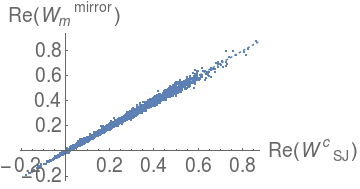
(e) $m=1$

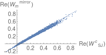
(f) $m=2$

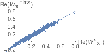
(g) $m=5$

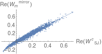
(h) $m=8$

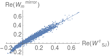
(i) $m=10$

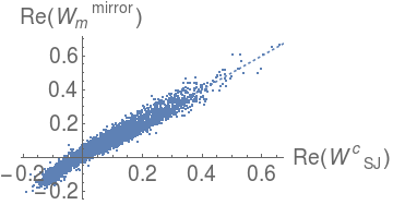
(j) $m=12$

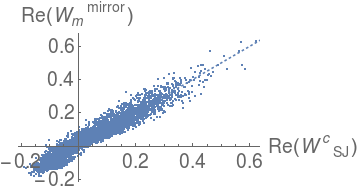
(k) $m=15$

Figure 19: A correlation plot of the real parts of $W^{c}_{SJ}$ vs $W^{\mathrm{mirror}}_{m}$ in the left-hand corner of the 2d causal diamond for a range of masses. The diagonal is denoted by a dotted line. As is evident, the correlation remains largely unchanged with mass. The increase in scatter with mass is related to the fact that the density of sprinkling is left unchanged.

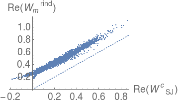
(a) $m=0.1$

(b) $m=0.2$

(c) $m=0.3$

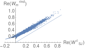
(d) $m=0.4$

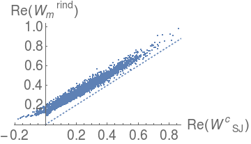
(e) $m=1$

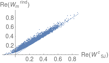
(f) $m=2$

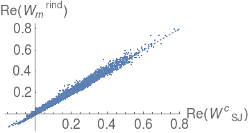
(g) $m=5$

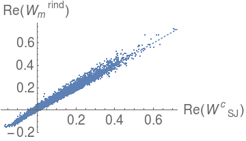
(h) $m=8$

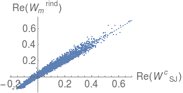
(i) $m=10$

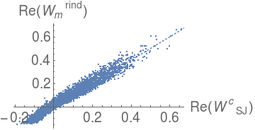
(j) $m=12$

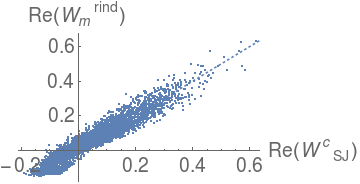
(k) $m=15$

Figure 20: A correlation plot of the real parts of $W^{c}_{SJ}$ vs $W^{\mathrm{rind}}_{m}$ for the same range of masses. For small masses, the correlation is poor but improves with mass.

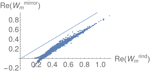
(a) $m=0.1$

(b) $m=0.2$

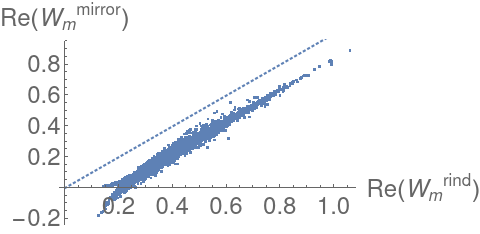
(c) $m=0.3$

(d) $m=0.4$

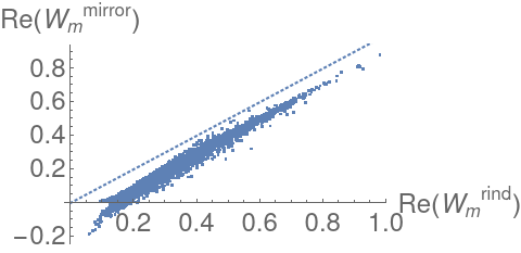
(e) $m=1$

(f) $m=2$

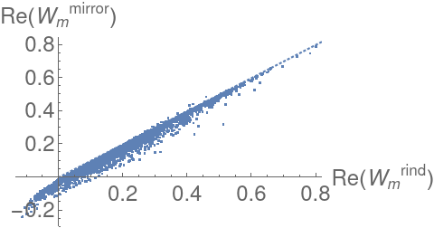
(g) $m=5$

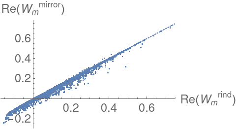
(h) $m=8$

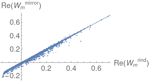
(i) $m=10$

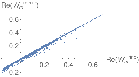
(j) $m=12$

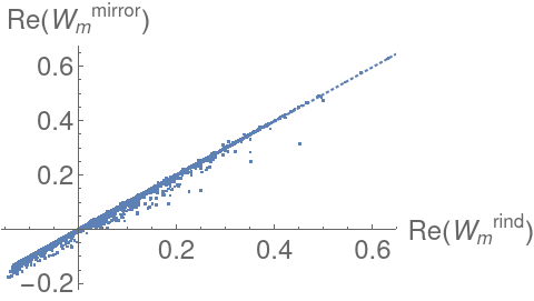
(k) $m=15$

Figure 21: A correlation plot of the real parts of $W^{\mathrm{mirror}}_{m}$ vs $W^{\mathrm{rind}}_{m}$ for the same range of masses. For small masses, the correlation is poor but improves with mass.

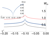
(a) $m=0.1$

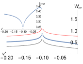
(b) $m=0.2$

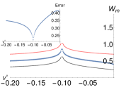
(c) $m=0.3$

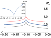
(d) $m=0.4$

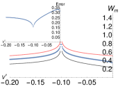
(e) $m=1$

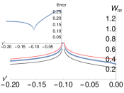
(f) $m=2$

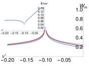
(g) $m=5$

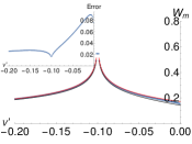
(h) $m=8$

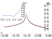
(i) $m=10$

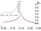
(j) $m=12$

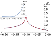
(k) $m=15$

Figure 22: Real parts of $W^{\mathrm{mink}}_{m}$ (red), $W^{\mathrm{rind}}_{m}$ (blue) and $W^{\mathrm{mirror}}_{m}$ (black) for a pair of points $(u=0.1,v=-0.1)$ and $(u^{\prime}=0.11,v^{\prime})$ with varying $v^{\prime}$. As the mass increases all three converge to a common value. To make the comparison explicit, the inset figure shows the relative error between the real parts of $W^{\mathrm{rind}}_{m}$ and $W^{\mathrm{mirror}}_{m}$ as a function of $v^{\prime}$.

References

[1]
R. D. Sorkin, “Scalar Field Theory on a Causal Set in Histories Form,” J. Phys. Conf. Ser., vol. 306, p. 012017, 2011.
[2]
S. Johnston, “Feynman Propagator for a Free Scalar Field on a Causal Set,”
Phys. Rev. Lett., vol. 103, p. 180401, 2009.
[3]
N. Afshordi, M. Buck, F. Dowker, D. Rideout, R. D. Sorkin, and Y. K. Yazdi,
“A Ground State for the Causal Diamond in 2 Dimensions,” JHEP,
vol. 10, p. 088, 2012.
[4]
S. P. Johnston, Quantum Fields on Causal Sets.
PhD thesis, Imperial Coll., London, 2010.
[5]
M. Buck, F. Dowker, I. Jubb, and R. Sorkin, “The Sorkin-Johnston state in a
patch of the trousers spacetime,” Class. Quant. Grav., vol. 34,
no. 5, p. 055002, 2017.
[6]
C. J. Fewster and R. Verch, “On a Recent Construction of ’Vacuum-like’
Quantum Field States in Curved Spacetime,” Class. Quant. Grav.,
vol. 29, p. 205017, 2012.
[7]
S. Surya, N. X, and Y. K. Yazdi, “Studies on the SJ Vacuum in de Sitter
Spacetime,” JHEP, vol. 07, p. 009, 2019.
[8]
N. Afshordi, S. Aslanbeigi, and R. D. Sorkin, “A Distinguished Vacuum State
for a Quantum Field in a Curved Spacetime: Formalism, Features, and
Cosmology,” JHEP, vol. 08, p. 137, 2012.
[9]
M. Brum and K. Fredenhagen, “‘Vacuum-like’ Hadamard states for quantum
fields on curved spacetimes,” Class. Quant. Grav., vol. 31,
p. 025024, 2014.
[10]
N. Avilan, A. F. Reyes-Lega, and B. Carneiro da Cunha, “Coupling the
Sorkin-Johnston State to Gravity,” Phys. Rev., vol. D90, no. 8,
p. 084036, 2014.
[11]
R. M. Wald, Quantum Field Theory in Curved Spacetime and Black Hole
Thermodynamics.
Chicago, USA: Chicago Univ. Pr., 1994.
[12]
R. D. Sorkin, “From Green Function to Quantum Field,” Int. J. Geom.
Meth. Mod. Phys., vol. 14, no. 08, p. 1740007, 2017.
[13]
M. R. Speigel, “The Summation of Series Involving Roots of Transcendental
Equations and Related Applications,” Journal of Applied Physics,
vol. 24, p. 1103, 1953.
[14]
E. Abdallah, M. C. B. Abdallah, and K. D. Rothe, ”Non-perturbative methods
in Two Dimensional Quantum Field Theory”.
Singapore: World Scientific Publishing Co., 2nd ed., 2001.
[15]
P. Candelas and D. J. Raine, “Quantum Field Theory on incomplete
manifolds,” Journal of Mathematical Physics, vol. 17, p. 2101, 1976.
[16]
L. Bombelli, J. Lee, D. Meyer, and R. Sorkin, “Space-Time as a Causal Set,”
Phys. Rev. Lett., vol. 59, pp. 521–524, 1987.
[17]
S. Surya, “The causal set approach to quantum gravity.” arXiv:1903.11544,
2019.
[18]
S. Johnston, “Particle propagators on discrete spacetime,” Class.
Quant. Grav., vol. 25, p. 202001, 2008.
[19]
Y. K. Yazdi, “A Spacetime Approach to Defining Vacuum States and Entropy,”
Master’s thesis, University of Waterloo, 2013.
[20]
H. Muneesamy, “Quantum Field Theory and Entanglement Entropy in a 2D Scalar
Causal Set,” Master’s thesis, Imperial Coll., London, 2021.
(a)
(b)
(a)
(b)