Replacing the do-calculus with Bayes rule

Abstract

The concept of causality has a controversial history. The question of whether it is possible to represent and address causal problems with probability theory, or if fundamentally new mathematics such as the do-calculus is required has been hotly debated, e.g. [Pearl, 2001] states ‘the building blocks of our scientific and everyday knowledge are elementary facts such as “mud does not cause rain” and “symptoms do not cause disease” and those facts, strangely enough, cannot be expressed in the vocabulary of probability calculus’. This has lead to a dichotomy between advocates of causal graphical modeling and the do-calculus, and researchers applying Bayesian methods. In this paper we demonstrate that, while it is critical to explicitly model our assumptions on the impact of intervening in a system, provided we do so, estimating causal effects can be done entirely within the standard Bayesian paradigm. The invariance assumptions underlying causal graphical models can be encoded in ordinary Probabilistic graphical models, allowing causal estimation with Bayesian statistics, equivalent to the do-calculus. Elucidating the connections between these approaches is a key step toward enabling the insights provided by each to be combined to solve real problems.

1 Introduction

The do-calculus [Pearl, 1995] is a powerful body of theory that provides three additional rules for probability theory on the basis that probability theory alone is not sufficient for solving causal problems (an argument prosecuted forcefully by Pearl in several places e.g. [Pearl, 2001]). In this paper we provide side by side analysis of four classic causal problems: the two cases responsible for Simpson’s reversal, and two cases with unobserved confounders. These four analyses are strongly suggestive that the do-calculus and Bayesian inference can both be used in order to make causal estimates, although this is not to suggest that each approach does not have its strengths and weaknesses.

A fully Bayesian approach leverages a vast body of existing research and is able to account for finite sample uncertainties. On the other hand the do-calculus has simpler graphs and is sometimes a more direct approach, also some of the results pertaining to unobserved confounders were discovered using the do-calculus (in particular results for front door adjustment and M-Bias) and while we show these results can be transferred in the Bayesian paradigm the mechanism for systematically doing so in a tractable manner remains unclear.

While there is much to be discussed about the similarities and differences between the two approaches we mostly leave this outside scope and simply provide the four examples side by side. The paper has the following structure, in Section 2 we outline the two methodologies in a sufficiently general framework that either could be used to solve causal problems. In Section 3 we outline the two fully observed problems, here we focus on Simpson’s paradox. In Section 4 we outline two problems involving unobserved confounders; the causality non-identifiable case and the front door rule; concluding remarks are made in Section 5.

2 Two schools of thought

2.1 Probabilistic graphical models

Probabilistic graphical models (PGMs) combine graph theory with probability theory in order to develop new algorithms and to present models in an intuitive framework [Jordan, 2004]. A Probabilistic graphical model is a directed acyclic graph over variables, which represents how the joint distribution over these variables may be factorized. In particular, any missing edge in the graph must correspond to a conditional independence relation in the joint distribution. There are multiple valid Probabilistic graphical model representations for a given joint distribution. For example, any joint distribution over two variables $(X,Y)$ may be represented by both $X\rightarrow Y$ or $X\leftarrow Y$.

2.2 Causal Graphical Models And The Do-Calculus

A causal graphical model (CGM) is a Probabilistic graphical model, with the additional assumption that a link $X\rightarrow Y$ means $X$ causes $Y$. Think of the data generating process for a CGM as sampling data first for the exogenous variables (those with no parents in the graph), and then in subsequent steps sampling values for the children of previously sampled nodes. An atomic intervention in such a system that sets the value of a specific variable $T$ to a fixed constant corresponds to removing all links into $T$ - as it is now set exogenously, rather than determined by its previous causes. It is assumed that everything else in the system remains unchanged, in particular the functions or conditional distributions that determine the value of a variable given its parents in the graph. In this way, a CGM encodes more than the factorization (or conditional independence structure) of the joint distribution over its variables; It additionally specifies how the system responds to atomic interventions.

A CGM describes how the structure of a system is modified by an intervention. However, answering causal queries such as "what would the distribution of cancer look like if we were able to prevent smoking?" requires inference about the distributions of variables in the post-interventional system. The do-notation is a short-hand for describing the distribution of variables post-intervention and the do-calculus is a set of rules for identifying which (conditional) distributions are equivalent pre and post-intervention. If it is possible to derive an expression for the desired post-interventional distribution purely in terms of the joint distribution over the original system via the do-calculus then the causal query is identifiable, meaning assuming positive density and infinite data we obtain a point estimate for it. The do-calculus is complete; A query is identifiable if and only if it can be solved via the do-calculus [Shpitser and Pearl, 2006, Huang and Valtorta, 2006].

Here we present the do-calculus in a simplified form that applies to interventions on single variables - which is sufficient for the examples presented in this paper. The full form of the do-calculus applies to interventions on any subset of variables - see [Pearl, 1995, Pearl, 2009, Peters et al., 2017].

The do-calculus

Let $G$ be a CGM, ${\color[rgb]{0.375,0.73046875,0.2734375}G_{\overline{T}}}$ represent $G$ post-intervention (i.e with all links into $T$ removed) and $G_{\underline{T}}$ represent $G$ with all links out of $T$ removed. Let $do(t)$ represent intervening to set a single variable $T$ to $t$,

Rule 1:

$\mathbb{P}(y|do(t),z,w)=\mathbb{P}(y|do(t),z)$ if $Y\perp\!\!\!\perp W|(Z,T)$ in ${\color[rgb]{0.375,0.73046875,0.2734375}G_{\overline{T}}}$

Rule 2:

$\mathbb{P}(y|do(t),z)=\mathbb{P}(y|t,z)$ if $Y\perp\!\!\!\perp T|Z$ in ${\color[rgb]{0.98046875,0.6171875,0}G_{\underline{T}}}$

Rule 3:

$\mathbb{P}(y|do(t),z)=\mathbb{P}(y|z)$ if $Y\perp\!\!\!\perp T|Z$ in ${\color[rgb]{0.375,0.73046875,0.2734375}G_{\overline{T}}}$, and $Z$ is not a decedent of $T$.

2.3 Representing a Causal Problem with a Probabilistic graphical model

While PGMs and CGMs may appear similar, there are key differences between them, both in the information they represent and how they are typically applied. CGMs are used to determine if a given query is identifiable and to obtain an expression for it in terms of the original joint distribution - with estimation of this expression a follow up step; latent variables are introduced to capture dependence induced by unobserved variables that may complicate identification of causal effects and links are not reversible. By contrast in PGMs links can be reversed, model specific details for estimation - including plates & parameters - are included graphically, and latent variables (of a specific form) are introduced for computational reasons, usually to coerce the model into complete data exponential family form.

To represent an intervention with an ordinary Probabilistic graphical model, we must explicitly model the pre and post intervention systems and the relationship between them.

Algorithm 1: CausalBayesConstruct

Input: Causal graph $G$ and intervention $do(T=t)$.  
Output: Probabilistic graphical model representing this intervention

1. Draw the original causal graph $G$ inside a plate indexed from $1,...M$ to represent the data generating process.

2. For each variable $V\in G$, parameterize $P(V|parents(V))$ by adding a parameter $\theta_{V}$ with a link into $V$.

3. Draw the graph after the intervention by setting $T=t$ and removing all links into it. Rename each of the variables to distinguish them from the variables in the original graph, e.g. $X$ becomes $X^{*}$.

4. Connect the two graphs linking $\theta_{V}$ to the corresponding variable $V^{*}$ in the post-interventional graph, for each $V$ excluding $T$.

A PGM constructed with Algorithm 1 represents exactly the same assumptions about a specific intervention as the corresponding CGM, see Figures 1 and 3 for an example. We have just explicitly created a joint model over the system pre and post-intervention, which allows the direct application of standard statistical inference, rather than requiring additional notation and operations that map from one to the other - as the do-calculus does. The Bayesian model is specified by the parameterization of the conditional distribution of variables given their parents, and priors may be placed on the parameters $\boldsymbol{\theta}$. The fact that the parameters are shared for all pairs of variables $(V,V^{*})$ excluding $T$, captures the assumption that all that is changed by the intervention is the way $T$ takes its value - the conditional distributions for all other variables given their parents are invariant.

Despite its simplicity we are unaware of a direct statement of Algorithm 1, it is related to twin networks [Pearl, 2009] and augmented directed acyclic graphs [Dawid, 2015] but is distinct from both.

2.4 Causal Inference with Probabilistic graphical models

The result of Algorithm 1 is a Probabilistic graphical model on which we can do inference with standard probability theory rather than the do-calculus, and which has properties such as arrow reversal (by the use of Bayes rule). To infer causal effects we compute a predictive distribution for the quantity of interest in the post-intervention graph using Bayes rule, integrating out all parameters, latent variables and any observed variables that are not of interest, for each setting of the treatment $T=t^{*}$.

To make this procedure clearer, let $\boldsymbol{V}$ be the set of variables in the original causal graph ${\color[rgb]{0.08984375,0.28515625,0.703125}G}$, excluding the variable we intervene on, $T$, and $\boldsymbol{V^{*}}$ be the corresponding variables in the post-interventional graph. We have:

• $\boldsymbol{\theta}$: the set of model parameters.

• $\boldsymbol{v}$: a matrix of the $M$ observations of variables $\boldsymbol{V}$, $(\boldsymbol{v}_{1},...,\boldsymbol{v}_{M})$ collected pre-intervention.

• $\boldsymbol{t}$: a vector of the $M$ observed values of the treatment variable $T$, $t_{1},..t_{M}$, and

• $\boldsymbol{v^{*}}$: The variables of the system post-intervention.

• $t^{*}$: the value that the intervened on variable $T$ is set to.

• $Y^{*}\in{\boldsymbol{v^{*}}}$: the variable of interest post-intervention.

The goal is to infer the value of the unobserved post-interventional distribution over $\boldsymbol{v^{*}}$, given the observed data and $(\boldsymbol{v},\boldsymbol{t})$ and a selected treatment $t^{*}$. By construction, conditional on the parameters $\boldsymbol{\theta}$, the post-interventional variables $\boldsymbol{v^{*}}$ are independent of data collected pre-intervention $(\boldsymbol{v},\boldsymbol{t})$. The value of the intervention $t^{*}$ is set exogenously - so is independent of both $\boldsymbol{\theta}$ and $(\boldsymbol{v},\boldsymbol{t})$. This ensures joint distribution over $(\boldsymbol{v},\boldsymbol{t},\boldsymbol{v^{*}},\boldsymbol{\theta})$ factorize into three terms: a prior over the parameters $\mathbb{P}(\boldsymbol{\theta})$, the likelihood for the original system $\mathbb{P}(\boldsymbol{v},\boldsymbol{t}|\boldsymbol{\theta})$, and a predictive distribution for the post-interventional variables given parameters and intervention $\mathbb{P}(\boldsymbol{v^{*}}|\boldsymbol{\theta},t^{*})$:

$$\mathbb{P}(\boldsymbol{v},\boldsymbol{t},\boldsymbol{v^{*}},\boldsymbol{\theta}|t^{*})=\mathbb{P}(\boldsymbol{\theta})\mathbb{P}(\boldsymbol{v},\boldsymbol{t}|\boldsymbol{\theta})\mathbb{P}(\boldsymbol{v^{*}}|\boldsymbol{\theta},t^{*})$$

We then marginalize out $\boldsymbol{\theta}$,

$$\mathbb{P}(\boldsymbol{v},\boldsymbol{t},\boldsymbol{v^{*}}|t^{*})=\int_{\boldsymbol{\theta}}\mathbb{P}(\boldsymbol{\theta})\mathbb{P}(\boldsymbol{v},\boldsymbol{t}|\boldsymbol{\theta})\mathbb{P}(\boldsymbol{v^{*}}|\boldsymbol{\theta},t^{*})d\boldsymbol{\theta}$$ (1)

and condition on the observed data $(\boldsymbol{v},\boldsymbol{t})$,

$$\mathbb{P}(\boldsymbol{v^{*}}|\boldsymbol{v},\boldsymbol{t},t^{*}) =\frac{\mathbb{P}(\boldsymbol{v},\boldsymbol{t},\boldsymbol{v^{*}}|t^{*})}{\mathbb{P}(\boldsymbol{v},\boldsymbol{t}|t^{*})}$$

$$=\int_{\boldsymbol{\theta}}\frac{\mathbb{P}(\boldsymbol{\theta})\mathbb{P}(\boldsymbol{v},\boldsymbol{t}|\boldsymbol{\theta})}{\mathbb{P}(\boldsymbol{v},\boldsymbol{t})}\mathbb{P}(\boldsymbol{v^{*}}|\boldsymbol{\theta},t^{*})d\boldsymbol{\theta}$$

$$=\int_{\boldsymbol{\theta}}\mathbb{P}(\boldsymbol{\theta}|\boldsymbol{v},\boldsymbol{t})\mathbb{P}(\boldsymbol{v^{*}}|\boldsymbol{\theta},t^{*})d\boldsymbol{\theta}.$$ (2)

Finally, if the goal is to infer mean treatment effects on a specific variable post-intervention $Y^{*}$, we can marginalize out the remaining variables in $\boldsymbol{V^{*}}$,

$$\mathbb{P}(Y^{*}|\boldsymbol{v},\boldsymbol{t},t^{*}) =\int_{\boldsymbol{\theta}}\mathbb{P}(\boldsymbol{\theta}|\boldsymbol{v},\boldsymbol{t})\sum_{\boldsymbol{V^{*}}\backslash Y^{*}}\mathbb{P}(\boldsymbol{v^{*}}|\boldsymbol{\theta},t^{*})d\boldsymbol{\theta}.$$ (3)

If there are no latent variables in ${\color[rgb]{0.08984375,0.28515625,0.703125}G}$, assuming positive density over the domain of $(\boldsymbol{v},\boldsymbol{t})$ and a well defined prior $\mathbb{P}(\boldsymbol{\theta})$, the likelihood $\mathbb{P}(\boldsymbol{v},\boldsymbol{t}|\boldsymbol{\theta})$ will dominate, and the posterior over the parameters $\mathbb{P}(\boldsymbol{\theta}|\boldsymbol{v},\boldsymbol{t})$ will become independent of the prior at the infinite data limit. The term $\mathbb{P}(\boldsymbol{v^{*}}|\boldsymbol{\theta},t^{*})$ can be expanded into a product of terms of the form $\mathbb{P}(V^{*}|parents(V^{*}),\boldsymbol{\theta})$ following the factorization implied by the post-interventional graph. From step (3) of Algorithm 1 each of these terms are equal to the corresponding terms $\mathbb{P}(V|parents(V),\boldsymbol{\theta})$, giving results equivalent to Pearl’s truncated product formula [Pearl, 2009].

The presence of latent variables in ${\color[rgb]{0.08984375,0.28515625,0.703125}G}$ adds complications which we defer to Section 4.

3 Simpson’s Paradox (Fully Observed)

Simpson’s paradox provides an excellent case study for demonstrating that raw data cannot be used for inferring causality without further assumptions. In this section, we show how we can infer treatment effects and resolve the paradox, with either the do-calculus or via Bayesian inference, and that these approaches yield equivalent results. Assume we have a table of data on some outcome $Y$ for two different treatments ($T$) broken down by a third variable $Z$ as shown in Table 1.

$z$	$t$	$y$	$N$
0	0	0	150
0	0	1	50
0	1	0	180
0	1	1	180
1	0	0	50
1	0	1	200
1	1	0	4
1	1	1	36

Table 1: Example Data

By estimating probabilities as past frequencies we obtain the following conditional probabilities:

$$P(Y=1|Z=0,T=0)=0.25$$

$$P(Y=1|Z=0,T=1)=0.5$$

$$P(Y=1|Z=1,T=0)=0.8$$

$$P(Y=1|Z=1,T=1)=0.9$$

$P(Y=1|T=0)=0.56$

$P(Y=1|T=1)=0.54$

The paradox

Treatment $T=0$ seems best overall, but if we break the data down by $Z$ then, regardless of which value of $Z$ a patient has, treatment $T=1$ seems better. If we had to select a single treatment for everyone - which should it be? The key to resolving this question is to realize that what we care about in this setting is the expected outcome of intervening in the system to set $T$, (in Pearl’s notation $\mathbb{P}(Y|do(T))$) rather than either of the conditional distributions $\mathbb{P}(Y|T)$ or $\mathbb{P}(Y|T,Z)$. As a result, which treatment is preferred hinges on causal assumptions, which we may specify using a CGM or a PGM.

3.1 Simpson’s Paradox Case 1

Figure 1: A CGM of Case 1: Left observational, Right: mutilated

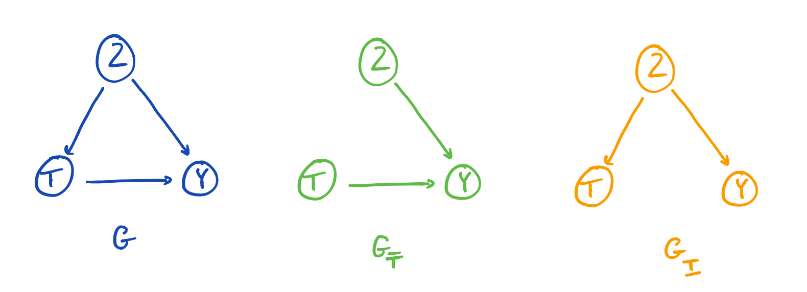
Figure 2: The graphs ${\color[rgb]{0.08984375,0.28515625,0.703125}G}$, ${\color[rgb]{0.375,0.73046875,0.2734375}G_{\overline{T}}}$ and ${\color[rgb]{0.98046875,0.6171875,0}G_{\underline{T}}}$ for case 1.

Figure 3: A PGM of Case 1

Imagine that our observations are generated by CGM given in Figure 1, where the covariate $Z$ is a cause of both $T$ and $Y$. Applying the rules of the do-calculus gives:

$$\mathbb{P}( y|do(T=t))=\sum_{z}\mathbb{P}(y,z|do(T=t))$$

$$=\sum_{z}\mathbb{P}(y|do(T=t),z)\mathbb{P}(z|do(T=t))$$

$$=\sum_{z}\underbrace{\mathbb{P}(y|t,z)}_{\text{Rule 2:($Y\perp\!\!\!\perp T|Z$ in ${\color[rgb]{0.98046875,0.6171875,0}G_{\underline{T}}}$) }}\underbrace{\mathbb{P}(z)}_{\text{Rule 3:($Z\perp\!\!\!\perp T$ in ${\color[rgb]{0.375,0.73046875,0.2734375}G_{\overline{T}}}$)}}$$

See Figure 2 for ${\color[rgb]{0.08984375,0.28515625,0.703125}G}$, ${\color[rgb]{0.375,0.73046875,0.2734375}G_{\overline{T}}}$ and ${\color[rgb]{0.98046875,0.6171875,0}G_{\underline{T}}}$ in case 1.

To find the same solution using a Bayesian approach we first apply CausalBayesConstruct on CGM Figure 1 to produce the PGM in Figure 3. We then explicitly parameterize the model and write out the three model components, the post intervention predictive, the likelihood component and the prior component.

We use the following parameterization:

$$\mathbb{P}(y|t,z,\boldsymbol{\psi})=\boldsymbol{\psi}_{t,z}^{y}(1-\boldsymbol{\psi}_{t,z})^{1-y}=\mathbb{P}(y^{*}|t^{*},z^{*},\boldsymbol{\psi}),$$

$$\mathbb{P}(z|\boldsymbol{\gamma})=\boldsymbol{\gamma}^{z}(1-\boldsymbol{\gamma})^{1-z}=\mathbb{P}(z^{*}|\boldsymbol{\gamma}),$$

$$\mathbb{P}(t|z,\boldsymbol{\phi})=\boldsymbol{\phi}_{z}^{t}(1-\boldsymbol{\phi}_{z})^{1-t}.$$

The post intervention predictive is:

$$\mathbb{P}(y^{*}|t^{*},\boldsymbol{\psi},\boldsymbol{\gamma})= \sum_{z^{*}}\mathbb{P}(y^{*}|t^{*},z^{*},\boldsymbol{\psi})\mathbb{P}(z^{*}|\boldsymbol{\gamma}).$$

$$= \sum_{z}\boldsymbol{\psi}_{t^{*},z}^{y^{*}}(1-\boldsymbol{\psi}_{t^{*},z})^{1-y^{*}}\boldsymbol{\gamma}^{z}(1-\boldsymbol{\gamma})^{1-z}$$

The likelihood component is:

$$\mathbb{P}( \boldsymbol{y}|\boldsymbol{t},\boldsymbol{z},\boldsymbol{\psi})\mathbb{P}(\boldsymbol{t}|\boldsymbol{z},\boldsymbol{\phi})\mathbb{P}(\boldsymbol{z}|\boldsymbol{\gamma})$$

$$= \prod_{m}\boldsymbol{\psi}_{t_{m},z_{m}}^{y_{m}}(1-\boldsymbol{\psi}_{t_{m},z_{m}})^{1-y_{m}}$$

$$\times\boldsymbol{\phi}_{z_{m}}^{t_{m}}(1-\boldsymbol{\phi})^{1-z_{m}}\boldsymbol{\gamma}^{z_{m}}(1-\boldsymbol{\gamma})^{1-z_{m}}$$

By de Finetti’s strong law of large numbers [De Finetti, 1980] as $M\rightarrow\infty$ the posterior concentrate on a single point $\hat{\boldsymbol{\psi}},\hat{\boldsymbol{\phi}},\hat{\boldsymbol{\gamma}}$ and ${\hat{\boldsymbol{\psi}}_{t,z}^{y}(1-\hat{\boldsymbol{\psi}}_{t,z})^{1-y}\rightarrow\mathbb{P}(y|t,z)}$ and ${\hat{\boldsymbol{\gamma}}^{z}(1-\hat{\boldsymbol{\gamma}})^{1-z}\rightarrow\mathbb{P}(z)}$, consequently:

$${\rm lim}_{M\rightarrow\infty}\sum_{z}\hat{\boldsymbol{\psi}}_{t^{*},z}^{y^{*}}(1-\hat{\boldsymbol{\psi}}_{t^{*},z^{*}})^{1-y^{*}}\hat{\boldsymbol{\gamma}}^{z}(1-\hat{\boldsymbol{\gamma}})^{1-z}$$

$$\rightarrow\sum_{z}\mathbb{P}(y|t,z)\mathbb{P}(z).$$

Which demonstrates the agreement between the Bayesian solution and the solution found using the do-calculus at large samples.

This convergence is usually very fast and good agreement will also be found for low sample sizes (where instead of using the point estimate we integrate over the posterior) e.g. under uniform priors the posterior of the parameters will have Beta distributions; and the predictive distribution giving the causal inference can be computed using the “Laplace smoothing algorithm” which involves adding one to the counts before normalizing.

Returning to the numerical example applying the do-calculus using the maximum likelihood algorithm we obtain:

$$\mathbb{P}( y|do(T=t))$$

$$=\mathbb{P}(y|t,Z=0)\mathbb{P}(Z=0)+\mathbb{P}(y|t,Z=1)\mathbb{P}(Z=1)$$

so

$$\mathbb{P}(Y=1|do(T=0)) =\frac{50}{200}\frac{560}{850}+\frac{200}{250}\frac{290}{850}$$

$$\approx 0.4376471$$

$$\mathbb{P}(Y=1|do(T=1)) =\frac{180}{360}\frac{560}{850}+\frac{36}{40}\frac{290}{850}$$

$$\approx 0.6364706$$

Assuming uniform priors and applying the Bayesian solution we obtain:

$$\mathbb{P}(Y^{*}=1|T^{*}=0,\boldsymbol{t},\boldsymbol{y},\boldsymbol{z}) =\frac{51}{202}\frac{561}{852}+\frac{201}{252}\frac{291}{852}$$

$$\approx 0.4386687$$

$$\mathbb{P}(Y^{*}=1|T^{*}=1,\boldsymbol{t},\boldsymbol{y},\boldsymbol{z}) =\frac{181}{362}\frac{561}{852}+\frac{37}{42}\frac{291}{852}$$

$$\approx 0.630114$$

We see good agreement between the two methods with the only difference being the prior impact due to the finite sample. We also see that $T=1$ is the better treatment (assuming that $Y=1$ is the desired outcome).

4 Simpson’s Paradox Case 2

Figure 4: A CGM of Case 2: Left observational, Right: mutilated

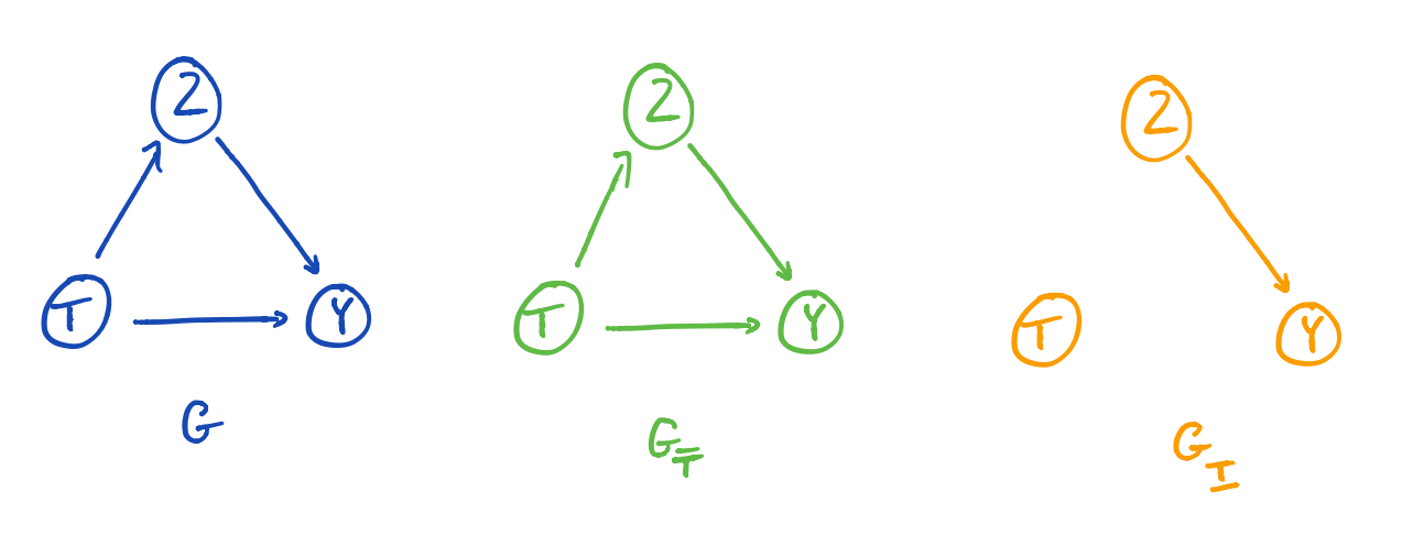
Figure 5: The graphs ${\color[rgb]{0.08984375,0.28515625,0.703125}G}$, ${\color[rgb]{0.375,0.73046875,0.2734375}G_{\overline{T}}}$ and ${\color[rgb]{0.98046875,0.6171875,0}G_{\underline{T}}}$ for case 2.

Imagine that our observations are generated by CGM given in Figure 4. Using the do-calculus we get the result in one step:

$$\underbrace{\mathbb{P}(y|do(T=t))=\mathbb{P}(y|T=t)}_{\text{Rule 2}}\text{, since }Y\perp\!\!\!\perp T\text{ in }{\color[rgb]{0.98046875,0.6171875,0}G_{\underline{T}}}$$

$$=\sum_{z}\mathbb{P}(y,z|t)$$

see Figure 5 to see the meaning of ${\color[rgb]{0.98046875,0.6171875,0}G_{\underline{T}}}$.

Figure 6: A PGM of Case 2

To find the same solution using a Bayesian approach we first apply CausalBayesConstruct on CGM Figure 4 to produce the PGM in Figure 6. We then explicitly parameterize the model and write out the three model components, the post intervention predictive, the likelihood component and the prior component.

We use the following parameterization:

$$\mathbb{P}(y|t,z,\boldsymbol{\psi})=\boldsymbol{\psi}_{t,z}^{y}(1-\boldsymbol{\psi}_{t,z})^{1-y}=\mathbb{P}(y^{*}|t^{*},z^{*},\boldsymbol{\psi}),$$

$$\mathbb{P}(z|t,\boldsymbol{\gamma})=\boldsymbol{\gamma}_{t}^{z}(1-\boldsymbol{\gamma}_{t})^{1-z}=\mathbb{P}(z^{*}|t^{*},\boldsymbol{\gamma}),$$

$$\mathbb{P}(t|\boldsymbol{\phi})=\boldsymbol{\phi}^{t}(1-\boldsymbol{\phi})^{1-t}.$$

The post intervention predictive is:

$$\mathbb{P}( y^{*}|t^{*},\boldsymbol{\psi},\boldsymbol{\gamma})=$$

$$=\sum_{z^{*}}\mathbb{P}(y^{*}|t^{*},z^{*},\boldsymbol{\psi})\mathbb{P}(z^{*}|t^{*},\boldsymbol{\gamma})$$

$$=\sum_{z}\boldsymbol{\psi}_{t,z}^{y}(1-\boldsymbol{\psi}_{t,z})^{1-y}\boldsymbol{\gamma}_{t}^{z}(1-\boldsymbol{\gamma}_{t})^{1-z}$$

The likelihood component is:

$$\mathbb{P}( \boldsymbol{y}|\boldsymbol{t},\boldsymbol{z},\boldsymbol{\psi})\mathbb{P}(\boldsymbol{z}|\boldsymbol{t},\boldsymbol{\gamma})\mathbb{P}(\boldsymbol{t}|\boldsymbol{\phi})=$$

$$\prod_{m}\boldsymbol{\psi}_{t_{m},z_{m}}^{y_{m}}(1-\boldsymbol{\psi}_{t_{m},z_{m}})^{1-y_{m}}$$

$$\times\boldsymbol{\gamma}_{t_{m}}^{z_{m}}(1-\boldsymbol{\gamma}_{t_{m}})^{1-z_{m}}\boldsymbol{\phi}^{t_{m}}(1-\boldsymbol{\phi})^{1-t_{m}}$$

Again by de Finetti’s strong law of large numbers as $M\rightarrow\infty$ the the posterior concentrate on a single point $\hat{\boldsymbol{\psi}},\hat{\boldsymbol{\phi}},\hat{\boldsymbol{\gamma}}$ and ${\hat{\boldsymbol{\psi}}_{t,z}^{y}(1-\hat{\boldsymbol{\psi}}_{t,z})^{1-y}\rightarrow\mathbb{P}(y|t,z)}$ and ${\hat{\boldsymbol{\gamma}}_{t}^{z}(1-\hat{\boldsymbol{\gamma}}_{t})^{1-z}\rightarrow\mathbb{P}(z|t)}$, consequently:

$${\rm lim}_{M\rightarrow\infty}\sum_{z}\hat{\boldsymbol{\psi}}_{t^{*},z}^{y^{*}}(1-\hat{\boldsymbol{\psi}}_{t^{*},z})^{1-y^{*}}\hat{\boldsymbol{\gamma}}_{t^{*}}^{z}(1-\hat{\boldsymbol{\gamma}}_{t^{*}})^{1-z}$$

$$\rightarrow\sum_{z}\mathbb{P}(y,z|t)$$

Showing that again there is large sample agreement between the two methods, Similarly, convergence is usually very fast and there is close agreement for even small samples.

Returning to the numerical example applying the do-calculus using the maximum likelihood algorithm we obtain:

$$\mathbb{P}(Y=1|do(T=0))=\frac{250}{450}\approx 0.5555556$$

$$\mathbb{P}(Y=1|do(T=1)) =\mathbb{P}(y|t)=\frac{216}{400}$$

$$\approx 0.54$$

Assuming uniform priors and applying the Bayesian solution again using the Laplace smoothing result we obtain:

$$\mathbb{P}(Y^{*}=1|T^{*}=0,\boldsymbol{t},\boldsymbol{y},\boldsymbol{z}) =\frac{51}{202}\frac{201}{452}+\frac{201}{252}\frac{251}{452}$$

$$\approx 0.5551989$$

$$\mathbb{P}(Y^{*}=1|T^{*}=1,\boldsymbol{t},\boldsymbol{y},\boldsymbol{z}) =\frac{181}{362}\frac{361}{402}+\frac{37}{42}\frac{41}{402}$$

$$\approx 0.5388534$$

Again we see good agreement between the two methods with the only difference being the prior impact due to the finite sample. We also see that $T=0$ is the better treatment.

Note that the distribution over $\mathbb{P}(z,t,y)$ is identical for both Case 1 and Case 2, and yet the optimal treatment differs. The paradox is resolved by understanding that the difference is due to different model assumptions about the impact of intervening on $T$, and we have demonstrated that these assumptions can be expressed either with a CGM or an extended PGM.

5 With Unobserved Confounders

Unobserved confounders (or latent variables) are hidden variables that can complicate causal inference at best and at worst render it impossible. While a direct attack using the pre-specified methodology does allow Bayesian inference to solve these problems, this is achieved by marginalizing out a complex latent variable the size of which grows with the data set. Usually the inclusion of the latent variable is not viable and the model must be marginalize to remove it and re-parameterized. Whether this is possible in a way that allows causation to be identified depends on the structure of the graph. If it isn’t possible to identify all parameters that have a causal impact then prior distributions will have an impact even in the large data limit.

5.1 When Causality Cannot Be Identified

Figure 7: CGM Where Causality Is “not identifiable”: Left observational, Right: mutilated

Figure 8: PGM Where Causality Is “not identifiable”

The simplest graphical model where causation becomes impossible even with unlimited samples is shown in Figure 7. This fact is demonstrated in the do-calculus by the fact that there is no way to apply the 3 rules in order to obtain $\mathbb{P}(y|do(t))$.

In this problem we consider $T$ to be have two states and $Y$ to have two states, but the latent variable or unobserved confounder $Z$ is of arbitrary complexity. This reflects many real life problems e.g. $T$ could represent the presence of some substance in a person’s diet (so it is binary), $Y$ could represent some binary health outcome and $Z$ could represent socio-economic circumstances of a person affecting both $T$ and $Y$.

Following the same prescription as before; to find the same solution using a Bayesian approach we first apply CausalBayesConstruct on CGM Figure 7 to produce the PGM in Figure 8. We then explicitly parameterize the model and write out the three model components, the post intervention predictive component, the likelihood component and the prior component. The first step of parameterization is complicated by the fact that $Z$ is both latent and high dimensional this results in posteriors over the parameters that are not-identifiable and high dimensional, we will also consider a re-parameterization which partially mitigates these difficulties.

We use the following parameterization:

$$\mathbb{P}(y|t,z,\boldsymbol{\psi}) =\boldsymbol{\psi}_{t,z}^{y}(1-\boldsymbol{\psi}_{t,z})^{1-y}=\mathbb{P}(y^{*}|t^{*},z^{*},\boldsymbol{\psi})$$

$$\mathbb{P}(z|\boldsymbol{\gamma}) =\boldsymbol{\gamma}_{z^{*}}=\mathbb{P}(z^{*}|\boldsymbol{\gamma}),$$

$$\mathbb{P}(t|z,\boldsymbol{\phi}) =\boldsymbol{\phi}_{z}^{t}(1-\boldsymbol{\phi}_{z})^{1-t}.$$

The post intervention predictive is:

$$\mathbb{P}( y^{*}|t^{*},\boldsymbol{\psi},\boldsymbol{\gamma})=\sum_{z^{*}}P(y^{*}|t^{*},z^{*},\boldsymbol{\psi})P(z^{*}|\boldsymbol{\gamma})$$

$$=\sum_{z}\boldsymbol{\psi}_{t^{*},z}^{y^{*}}(1-\boldsymbol{\psi}_{t^{*},z})^{1-y^{*}}\boldsymbol{\gamma}_{z}$$

$$\equiv\boldsymbol{\Psi}_{t^{*},y^{*}}$$

We introduce the low dimensional $\boldsymbol{\Psi}$ as a re-parameterization of $\boldsymbol{\psi},\boldsymbol{\gamma}$ as statistically identifying this parameter is sufficient for making causal inference.

Unfortunately when we write the likelihood we see we cannot identify this parameter, but rather a different low dimensional function of $\boldsymbol{\psi},\boldsymbol{\phi},\boldsymbol{\gamma}$:

$$\mathbb{P}(y^{*},t^{*}|\boldsymbol{\psi},\boldsymbol{\phi},\boldsymbol{\gamma})$$

$$=\sum_{z}\mathbb{P}(y^{*}|t^{*},z,\boldsymbol{\psi})\mathbb{P}(t^{*}|z,\boldsymbol{\phi})\mathbb{P}(z|\boldsymbol{\gamma})$$

$$=\sum_{z}\boldsymbol{\psi}_{t^{*},z}^{y^{*}}(1-\boldsymbol{\psi}_{t^{*},z})^{1-y^{*}}\boldsymbol{\phi}_{z}^{t^{*}}(1-\boldsymbol{\phi}_{z})^{1-t^{*}}\boldsymbol{\gamma}_{z^{*}}$$

$$\equiv\boldsymbol{\Omega}_{t^{*},y^{*}}.$$

We introduce the low dimensional $\boldsymbol{\Omega}$ as a re-parameterization of $\boldsymbol{\psi},\boldsymbol{\phi},\boldsymbol{\gamma}$ as this parameter is identifiable.

We can now see the difficulty in this problem, we need $\boldsymbol{\Psi}$ but can only infer $\boldsymbol{\Omega}$. Both, $\boldsymbol{\Omega}$ and $\boldsymbol{\Psi}$ are different low dimensional projections of $(\boldsymbol{\psi},\boldsymbol{\phi},\boldsymbol{\gamma})$; $\boldsymbol{\Omega}$ is identifiable and $\boldsymbol{\Psi}$ is causally relevant, they are related due to the fact that they are both functions of $\boldsymbol{\psi}$ and $\boldsymbol{\gamma}$, so it may be reasonable to specify a joint prior $\mathbb{P}(\boldsymbol{\Psi},\boldsymbol{\Omega})$ giving:

$$\mathbb{P}( y^{*}|t^{*},\boldsymbol{y},\boldsymbol{t})$$

$$=\int_{\Psi}\int_{\boldsymbol{\Omega}}\mathbb{P}(y^{*}|t^{*},\boldsymbol{\Psi})\mathbb{P}(\boldsymbol{\Psi}|\boldsymbol{\Omega})\mathbb{P}(\boldsymbol{\Omega}|\boldsymbol{y},\boldsymbol{t})d\boldsymbol{\Omega}d\boldsymbol{\Psi}.$$

In specifying priors for this problem, we may reasonably use default priors (e.g. flat priors) for $\boldsymbol{\Omega}$ (or even take a point estimate) as it is identifiable with modest data sets. On the other hand $\mathbb{P}(\boldsymbol{\Psi}|\boldsymbol{\Omega})$ will be completely unaffected by the data so it is an extremely important that any information concerning on how $\boldsymbol{\Omega}$ affects knowledge of $\boldsymbol{\Psi}$ is carefully assessed; in many instances this will be considered too difficult to reasonably attempt, e.g. it may be that $\mathbb{P}(\boldsymbol{\Psi}|\boldsymbol{\Omega})=\mathbb{P}(\boldsymbol{\Psi})$ in which case the data adds no value to causal problems at all.

5.2 The Front Door Rule

Figure 9: A CGM for the Front Door Rule: Top the original graph, Bottom: the mutilated graph

Imagine that our observations are generated by the CGM given in Figure 9, which is the graph that requires the front door rule. The front door rule is remarkable in that it shows that a graph quite similar to Figure 7 does allow causation to be identifiable, the only difference being another observed node between the treatment and the outcome.

Using the do-calculus gives (detailed steps in [Pearl, 1995]):

$$\mathbb{P}(y|{\rm do}(T=t))=\sum_{w}\mathbb{P}(w|t)\sum_{t^{\prime}}\mathbb{P}(y|t^{\prime},w)\mathbb{P}(t^{\prime}).$$ (4)

Figure 10: A Bayesian Model for the Front Door Rule

To find the same solution using a Bayesian approach we first apply CausalBayesConstruct on CGM Figure 9 to produce the PGM in Figure 10. We then explicitly parameterize the model and write out the three model components. Again we are hampered by the presence of $u$, but for this problem we can effectively marginalize and re-parameterize the model to make causation identifiable.

We use the following parameterization:

$$\mathbb{P}(y|w,u,\boldsymbol{\psi})=\boldsymbol{\psi}_{w,u}^{y}(1-\boldsymbol{\psi}_{w,u})^{1-y}=\mathbb{P}(y^{*}|w^{*},u^{*},\boldsymbol{\psi}),$$

$$\mathbb{P}(w|t,\boldsymbol{\lambda})=\boldsymbol{\lambda}_{t}^{w}(1-\boldsymbol{\lambda}_{t})^{1-w}=\mathbb{P}(w^{*}|t^{*},\boldsymbol{\lambda}),$$

$$\mathbb{P}(u|\boldsymbol{\gamma})=\boldsymbol{\gamma}_{u}=\mathbb{P}(u^{*}|\boldsymbol{\gamma}),$$

$$\mathbb{P}(t|u,\boldsymbol{\phi})=\boldsymbol{\phi}_{u}^{t}(1-\boldsymbol{\phi}_{u})^{1-t}.$$

The post intervention predictive is:

$$\mathbb{P}( y^{*}|t^{*},\boldsymbol{\psi},\boldsymbol{\gamma},\boldsymbol{\lambda})$$

$$=\sum_{w^{*}}P(w^{*}|t^{*},\boldsymbol{\lambda})\sum_{u^{*}}\mathbb{P}(u^{*}|\boldsymbol{\gamma})\mathbb{P}(y^{*}|w^{*},u^{*},\boldsymbol{\psi}).$$

And the likelihood component is:

$$\mathbb{P}(\boldsymbol{y},\boldsymbol{t},\boldsymbol{w}|\boldsymbol{\psi},\boldsymbol{\lambda},\boldsymbol{\gamma},\boldsymbol{\phi})$$

$$= \prod_{m}\sum_{u_{m}}\boldsymbol{\psi}_{w_{m},u_{m}}^{y_{m}}(1-\boldsymbol{\psi}_{w_{m},u_{m}})^{1-y_{m}}\boldsymbol{\lambda}_{t_{m}}^{w_{m}}(1-\boldsymbol{\lambda})^{1-w_{m}}$$

$$\times\boldsymbol{\phi}^{t_{m}}(1-\boldsymbol{\phi})^{1-t_{m}}\boldsymbol{\gamma}_{u_{m}}.$$

Unfortunately, the fact that $u$ is both latent and large means that the posterior over $\boldsymbol{\psi},\boldsymbol{\gamma},\boldsymbol{\phi}$ is both non-identifiable and high dimensional (although the marginal posterior over $\boldsymbol{\lambda}$ is identifiable, since it depends only on $W$ and $T$). A direct attack would require sophisticated Bayesian approximation methods to capture the complex structure within the posterior and is not within the scope of this paper. Instead, we note that $u$ can be eliminated from the 2nd term in the post-intervention predictive distribution:

$$\sum_{u} \mathbb{P}(u|\boldsymbol{\gamma})\mathbb{P}(y|w,u,\boldsymbol{\psi})$$

$$= \sum_{u}\sum_{t}\mathbb{P}(u,t|\boldsymbol{\gamma},\boldsymbol{\phi})\mathbb{P}(y|w,u,\boldsymbol{\psi})$$

$$= \sum_{u}\sum_{t}\left(\frac{\mathbb{P}(u,t|\boldsymbol{\gamma},\boldsymbol{\phi})\mathbb{P}(w|t,\boldsymbol{\lambda})\mathbb{P}(y|w,u,\boldsymbol{\psi})}{\mathbb{P}(w|t,\boldsymbol{\lambda})}\right)$$

$$= \sum_{t}\left(\frac{\sum_{u}\mathbb{P}(u,t,w,y|\boldsymbol{\gamma},\boldsymbol{\phi},\boldsymbol{\lambda},\boldsymbol{\psi})}{\mathbb{P}(w|t,\boldsymbol{\lambda})}\right)$$

$$= \sum_{t}\frac{\mathbb{P}(t|\boldsymbol{\gamma},\boldsymbol{\phi})}{\mathbb{P}(w,t|\boldsymbol{\gamma},\boldsymbol{\phi},\boldsymbol{\lambda})}\mathbb{P}(y,t,w|\boldsymbol{\gamma},\boldsymbol{\phi},\boldsymbol{\lambda},\boldsymbol{\psi})$$

$$= \sum_{t}\mathbb{P}(t|\boldsymbol{\gamma},\boldsymbol{\phi})\mathbb{P}(y|t,w,\boldsymbol{\gamma},\boldsymbol{\phi},\boldsymbol{\lambda},\boldsymbol{\psi})$$

$$\neq \sum_{t}\mathbb{P}(y,t|w,\boldsymbol{\gamma},\boldsymbol{\phi},\boldsymbol{\lambda},\boldsymbol{\psi})~{}{\rm as}~{}\mathbb{P}(t|\boldsymbol{\gamma},\boldsymbol{\phi})\neq\mathbb{P}(t|w,\boldsymbol{\gamma},\boldsymbol{\phi})$$

We explicitly note this is not a joint distribution of $y,t|w$. Although it is a purely probabilistic expression, it is a distinctly Pearlian one. We re-parameterize:

$$\boldsymbol{\Omega}_{y,t,w}\equiv$$

$$\frac{\sum_{u}\boldsymbol{\psi}_{w,u}^{y}(1-\boldsymbol{\psi}_{w,u})^{1-y}\boldsymbol{\lambda}_{t}^{w}(1-\boldsymbol{\lambda}_{t})^{1-w}\boldsymbol{\phi}_{u}^{t}(1-\boldsymbol{\phi}_{u})^{1-t}\boldsymbol{\gamma}_{u}}{\boldsymbol{\lambda}_{t}^{w}(1-\boldsymbol{\lambda}_{t})^{1-w}}$$

This allows us to write the post-intervention predictive distribution as,

$$\mathbb{P}( y^{*}|t^{*},\boldsymbol{\Omega},\boldsymbol{\lambda})=\sum_{w}\boldsymbol{\lambda}_{t^{*}}^{w}(1-\boldsymbol{\lambda}_{t^{*}})^{1-w}\sum_{t}\boldsymbol{\Omega}_{y,t,,w}$$

$$= \sum_{u}\sum_{w}\boldsymbol{\psi}_{w,u}^{y}(1-\boldsymbol{\psi}_{w,u})^{1-y}\boldsymbol{\lambda}_{t}^{w}(1-\boldsymbol{\lambda}_{t})^{1-w}\boldsymbol{\gamma}_{u}$$

and the likelihood becomes,

$$\mathbb{P}(\boldsymbol{y},\boldsymbol{t},\boldsymbol{w}|\boldsymbol{\Omega},\boldsymbol{\lambda})=\prod_{m}\boldsymbol{\Omega}_{y_{m},t_{m},w_{m}}\boldsymbol{\lambda}_{t_{m}}^{w_{m}}(1-\boldsymbol{\lambda}_{t_{m}})^{1-w_{m}}.$$

As we have an expression for the causal quantities in terms of $\boldsymbol{\Omega},\boldsymbol{\lambda}$ we are able to identify the parameters needed to make causal estimates.

Finally we establish that the Bayesian solution converges to the unusual do-calculus expression given in Equation 4. The expression is unusual due to the fact that $t$ is both conditioned on and marginalized.

Again by de Finetti’s strong law of large numbers as as $M\rightarrow\infty$ the the posterior concentrate on a single point $\hat{\boldsymbol{\Omega}},\hat{\boldsymbol{\lambda}}$, consequently:

$${\rm lim}_{M\rightarrow\infty}\sum_{t^{\prime}}\hat{\boldsymbol{\Omega}}_{y,t^{\prime},w}\rightarrow\sum_{t^{\prime}}\mathbb{P}(t^{\prime})\mathbb{P}(y|t^{\prime},w)$$

and:

$${\rm lim}_{M\rightarrow\infty}\hat{\boldsymbol{\lambda}}_{t}^{w}(1-\hat{\boldsymbol{\lambda}}_{t})^{1-w}\rightarrow\mathbb{P}(w|t)$$

We once again obtain agreement with the Bayesian solution and the do-calculus:

$${\rm lim}_{M\rightarrow\infty}\sum_{w}\hat{\boldsymbol{\lambda}}_{t^{*}}^{w}(1-\hat{\boldsymbol{\lambda}}_{t^{*}})^{1-w}\sum_{t}\hat{\boldsymbol{\Omega}}_{y,t,w}$$

$$\rightarrow\sum_{w}\mathbb{P}(w|t)\sum_{t^{\prime}}\mathbb{P}(t^{\prime})\mathbb{P}(y|t^{\prime},w)$$

Again due to the rapid convergence there will be good agreement also for small samples.

6 Conclusion

The paper shows that it is possible to arrive at the same solution for causal problems using both the do-calculus and Bayesian theory, the key insight required for the Bayesian formulation is that the probabilistic graphical model must model both the pre-intervention and post intervention world separately, this is perhaps the major contribution we make otherwise our conclusion is similar to [Lindley et al., 1981]. Even though it has been long suggested that probability alone was insufficient for modeling causal systems (e.g. [Pearl, 1995, Pearl, 2001, Pearl, 2009, Pearl, 2014] ) it is perhaps unsurprising that Bayesian theory can accommodate these situations given its long history as arising from axiomizing reasoning under uncertainty (see [De Finetti, 1974, De Finetti, 1980, Lindley, 2000, Bernardo and Smith, 2009]).

There remains work to be done for a full unification. The key benefits of the Bayesian approach are correct finite sample behavior, and the ability to produce inference under situations which would be deemed unidentifiable under the do-calculus; this may be possible because Bayesian approaches are able to assume that conditional independence assumptions hold with high probability or approximately hold and then proceed, where the do-calculus applies hard tests of conditional independence.

The do-calculus has advantages in its ability to discard variables and reduce dimensionality and in its ability to identify re-parameterizations such as in the case of the front door rule which enable causality to be identifiable in surprising cases. Furthermore, the do-calculus is complete: we can obtain a point estimate for a causal query, without parametric assumptions on the model, if and only if we can express the query as a function of the observable, joint distribution pre-intervention via repeated application of the do-calculus and standard probability algebra [Huang and Valtorta, 2006, Shpitser and Pearl, 2006]. There is an algorithm [Shpitser and Pearl, 2012] that, for a given CGM and causal query, will determine if the query is identifiable via the do-calculus and; if it is, returns an expression for it in terms of the observable pre-interventional distribution. We speculate the algorithm could be adapted to the Bayesian context in order to automate the discovery of parameter transforms like the one we demonstrated for the front door rule.

A rich program of research is therefore open, some topics we think deserving of attention are: a comparison of the do-calculus and Bayesian approaches for instrumental variable models, CGM graphs where the do-calculus produces multiple solutions, CGM graphs where the do-calculus cannot identify but can produce bounds, CGM graphs where parametric assumptions are used in combination with the CGM in order to achieve identifiability and causal exploration where data is used to discover links before attempting a causal analysis. We hope other researchers will take up these challenges.

References

- [Bernardo and Smith, 2009] Bernardo, J. M. and Smith, A. F. (2009). Bayesian theory, volume 405. John Wiley & Sons.
- [Dawid, 2015] Dawid, A. P. (2015). Statistical causality from a decision-theoretic perspective. Annual Review of Statistics and Its Application, 2:273–303.
- [De Finetti, 1974] De Finetti, B. (1974). Theory of probability: A critical introductory treatment, volume 6. John Wiley & Sons.
- [De Finetti, 1980] De Finetti, B. (1980). Foresight: Its logical laws, its subjective sources (1937). Studies in subjective probability, pages 55–118.
- [Huang and Valtorta, 2006] Huang, Y. and Valtorta, M. (2006). Pearl’s calculus of intervention is complete. In Proceedings of the Twenty-Second Conference on Uncertainty in Artificial Intelligence, pages 217–224. AUAI Press.
- [Jordan, 2004] Jordan, M. I. (2004). Graphical models. Statistical Science, 19(1):140–155.
- [Lindley, 2000] Lindley, D. V. (2000). The philosophy of statistics. Journal of the Royal Statistical Society: Series D (The Statistician), 49(3):293–337.
- [Lindley et al., 1981] Lindley, D. V., Novick, M. R., et al. (1981). The role of exchangeability in inference. The Annals of Statistics, 9(1):45–58.
- [Pearl, 1995] Pearl, J. (1995). Causal diagrams for empirical research. Biometrika, 82(4):669–688.
- [Pearl, 2001] Pearl, J. (2001). Bayesianism and causality, or, why i am only a half-Bayesian. In Foundations of Bayesianism, pages 19–36. Springer.
- [Pearl, 2009] Pearl, J. (2009). Causality: Models, Reasoning, and Inference. Cambridge University Press, New York.
- [Pearl, 2014] Pearl, J. (2014). Comment: understanding Simpson’s paradox. The American Statistician, 68(1):8–13.
- [Peters et al., 2017] Peters, J., Janzing, D., and Schölkopf, B. (2017). Elements of causal inference: foundations and learning algorithms. MIT press.
- [Shpitser and Pearl, 2006] Shpitser, I. and Pearl, J. (2006). Identification of joint interventional distributions in recursive semi-markovian causal models. In Proceedings of the National Conference on Artificial Intelligence, volume 21, page 1219. Menlo Park, CA; Cambridge, MA; London; AAAI Press; MIT Press; 1999.
- [Shpitser and Pearl, 2012] Shpitser, I. and Pearl, J. (2012). Identification of conditional interventional distributions. In Proceedings of the twenty-second conference on uncertainty in artificial intelligence, pages 437–444. AUAI Press.