Lévy flights and hydrodynamic superdiffusion on the Dirac cone of Graphene

Abstract

We show that hydrodynamic collision processes of graphene at the neutrality point can be described in terms of a Fokker-Planck equation with fractional derivative, corresponding to a Lévy flight in momentum space. Thus, electron-electron collisions give rise to frequent small-angle scattering processes that are interrupted by rare large-angle events. The latter give rise to superdiffusive dynamics of collective excitations. We argue that such superdiffusive dynamics is of more general importance to the out-of-equilibrium dynamics of quantum-critical systems.

The kinetics of large gravitational systems such as globular clusters in galaxies or of a classical charged plasma are governed by continuous collisions with small-angle scatterings. The origin for this behavior is the long-range character of the Newton or Coulomb force, respectively. Such small-angle collisions behave in velocity space like drag and diffusion events, where a Fokker-Planck equation offers an efficient descriptionChandrasekhar1943 ; Rosenbluth1957 ; Chernoff1990 . Collisions can thus be seen as a Gaussian random walk in phase space. The velocity of a plasma or gravitational dust particle undergoes ordinary Brownian motion.

Quantum many-body systems that are near a quantum-critical point are governed by soft modes that will also induce effective long-range interactionsSachdevbook . This begs the question whether such quantum-critical systems also allow for an effective Fokker-Planck description of the non-equilibrium kinetics; in the collision-dominated hydrodynamic regime and in the crossover regime from hydrodynamic to ballistic dynamics. Candidate systems are itinerant electrons near magnetic or nematic quantum phase transitionsHertz1976 ; Moriya1984 ; Millis1993 ; Laughlin2001 ; Millis2002 ; Abanov2003 ; Loehneysen2007 ; DellAnna2007 ; Metlitski2010 ; Schattner2016 , the superconductor-insulator phase transitionDamle1997 , or graphene near the Dirac pointSheehy2007 . Anomalous diffusion was even shown to be present in two-dimensional Fermi liquidsGurzhi1995 ; Gurzhi1996 ; Maslov2011 ; Pal2012 ; Maslov2017 ; Ledwith2019 .

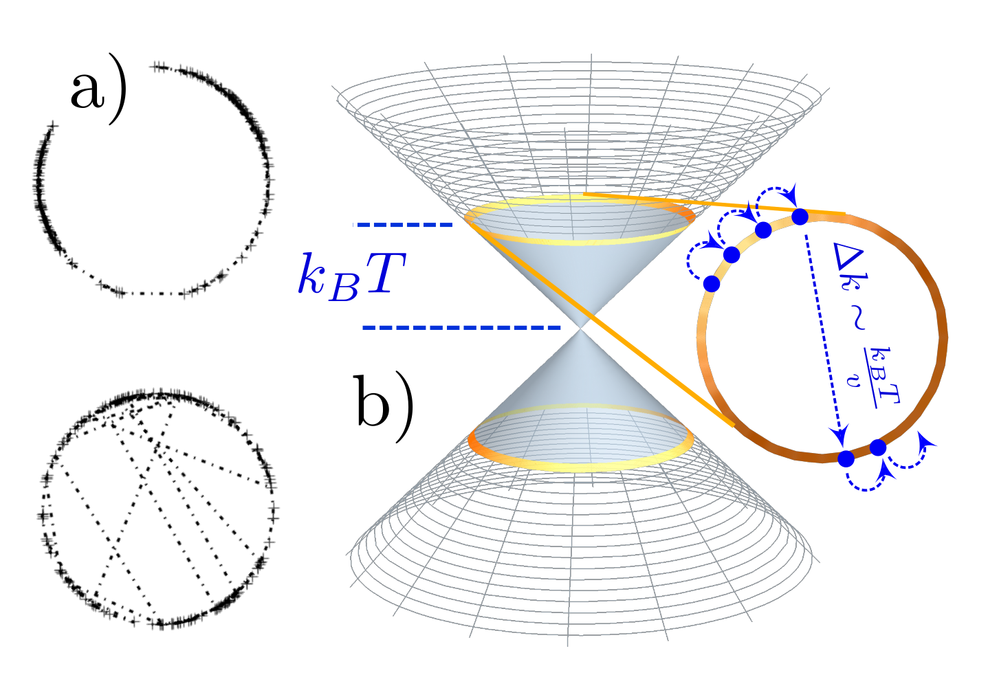
Figure 1: a) A wrapped Gaussian flight (upper circle) and a wrapped Cauchy flight (lower circle) with rare large momentum-transfer processes. b) Illustration of the Lévy flight in momentum space for graphene at the Dirac point. Electrons and holes that are thermally excited collide into each other. Most of the time the momentum transfer due to the electron-electron Coulomb interaction leads to small-angle scattering. However, those processes are interrupted by rare processes with large momentum transfer. The latter change the dynamics of the system qualitatively, leading to an accelerated or superdiffusive dynamics.

In this paper we analyze the quantum kinetics of graphene near the Dirac point with electron-electron Coulomb interaction. We show that the kinetic theory at charge neutralityFritz2008 ; Kashuba2008 ; Mueller2009 ; Schuett2011 ; Kiselev2019 can be expressed in terms of a Fokker-Planck equation, yet with fractional derivative with respect to the momentum direction. The underlying random processes are Lévy flightsLevy1954 ; Mandelbrot1977 ; Feller1972 , non-Gaussian random walks whose step widths are distributed according to a powerlaw. The slowly decaying tail of the step-width distribution makes it impossible to define a diffusion constant or to use a conventional Fokker-Planck equation. However, a diffusion equation of the form

$$\frac{\partial\rho}{\partial t}+D_{\mu}\left|\triangle\right|^{\frac{\mu}{2}}\rho=0,$$ (1)

with appropriately generalized fractional derivativeSamko1993 ; Hermann2014 can be used to describe such random walks. Lévy flights have been discussed to model the migration pattern of animals as they search for resourcesBartumeus2005 ; Reynolds2009 , the high-frequency index dynamics of the stock marketMantegna1997 , or to describe durations between consecutive earthquakesCorral2006 . In our system they correspond to random walks in momentum space with powerlaw weight for large momentum-transfer processes. We demonstrate that the collision operator due to electron-electron interactions in graphene takes the form of a fractional derivative. Then the Boltzmann equation becomes a fractional Fokker-Planck equation, similar to Eq.1 with exponent $\mu=1$:

$$\left(\partial_{t}+\mathbf{v}_{\mathbf{k}\lambda}\cdot\nabla_{\mathbf{x}}-\tau_{L}^{-1}\left(\frac{\partial^{2}}{\partial\theta^{2}}\right)^{1/2}\right)f_{\mathbf{k}\lambda}=S_{\mathbf{k}\lambda},$$ (2)

where $\theta$ determines the electron momentum direction: $\mathbf{k}=k\left(\cos\theta,\sin\theta\right)$. The precise definition of the fractional derivative is given below. This result implies that the out-of-equilibrium dynamics of graphene in the hydrodynamic regime is governed by a wrapped Cauchy flightLevy1939 ; Mardia1999 , a specific Lévy flight on the Dirac cone. In Fig. 1a we show a simulation of ordinary Brownian motion on a ring and of the wrapped Cauchy flight. Details of this simulation are summarized insupplementary material . The occurrence of rare large-angle jumps is clearly visible. The corresponding phase-space dynamics is sketched in Fig. 1b. While the direction of $\mathbf{k}$ undergoes anomalous diffusion, its magnitude $k\equiv\left|\mathbf{k}\right|$ is of the order of $k_{B}T/v_{0}$ with the graphene group velocity $v_{0}\approx 10^{8}{\rm cm}/{\rm s}$. The characteristic time of the process is $\tau_{L}$ with

$$\hbar\tau_{L}^{-1}\approx 11.66\alpha^{2}k_{B}T,$$ (3)

where the fine-structure constant of graphene is $\alpha=e^{2}/\left(\hbar\epsilon v_{0}\right)$. $\tau_{L}$ agrees up to a numerical coefficient with the collision time for the hydrodynamic transport behavior of graphene at the Dirac pointFritz2008 ; Kashuba2008 ; Mueller2009 . Below we discuss how $\tau_{L}$ is determined. Such a time scale was recently observed experimentally in THz spectroscopy of graphene at charge neutralityGallagher2019 .

Lévy flights in graphene have been discussed in Ref.Gattenloehner2016 , where an egineered distribution of adatoms was shown to result in a superdiffusive behavior of charge carriers, and in Ref.Briskot2014 in the context of highly photo-excited carriers that relax according to a cascade of processes - a behavior with interesting implications for pump-probe experiments. This can be seen as a superdiffusion in energy space far from equilibrium. It affects the magnitude of the momentum. Here we focus on the low-energy hydrodynamic regime and find a very different behavior for the directional diffusion in momentum space. Nevertheless, these results strongly suggest that superdiffusive phase-space dynamics is a more common phenomenon in quantum-critical systems.

We start from the Boltzmann equation

$$\left(\partial_{t}+\mathbf{v}_{\mathbf{k}\lambda}\cdot\nabla_{\mathbf{x}}+\mathbf{F}\left(\mathbf{x},t\right)\cdot\nabla_{\mathbf{k}}+{\cal C}\right)f_{\mathbf{k}\lambda}\left(\mathbf{x},t\right)=0$$ (4)

for the electron distribution function $f_{\mathbf{k}\lambda}\left(\mathbf{x},t\right)$ where $\mathbf{k}$ refers to the momentum and $\lambda=\pm 1$ labels the upper and lower cone of the Dirac spectrum $\varepsilon_{\mathbf{k}\lambda}=\lambda v_{0}\left|\mathbf{k}\right|$. $\mathbf{v}_{\mathbf{k}\lambda}=\partial\varepsilon_{\mathbf{k}\lambda}/\partial\mathbf{k}$ is the velocity vector and $\mathbf{F}\left(\mathbf{x},t\right)$ some external force, e.g. due to an external electric field. ${\cal C}$ is the Boltzmann collision operator due to electron-electron interactions and was derived to order $\alpha^{2}$ in Ref.Fritz2008 from a Keldysh-Schwinger approach; see also insupplementary material . It takes the usual form of a two-body interaction:

$${\cal C}f_{1} = -\sum_{2,3,4}W_{12,34}\left[f_{1}f_{2}\left(1-f_{3}\right)\left(1-f_{4}\right)\right|$$ (5)

$$- \left|\left(1-f_{1}\right)\left(1-f_{2}\right)f_{3}f_{4}\right].$$

The transition probability $W_{12,34}$ is due to the electron-electron Coulomb interaction $e^{2}/\epsilon$ of Dirac fermions that are confined to a two-dimensional system. $\epsilon$ is the dielectric constant determined by the substrate. For free standing graphene $\epsilon=1$ and the fine-structure constant $\alpha\approx 2.2$ is of order unity. A renormalization group analysis shows that $\alpha$ flows towards weak coupling, justifying our perturbative approachSheehy2007 .

As usual, the kinetic distribution function $f_{\lambda,\bm{k}}$ is expanded around the local equilibrium distribution $f_{k\lambda}^{0}=\left(e^{\beta\left(\epsilon_{\lambda,\bm{k}}-\mu\right)}+1\right)^{-1}$ and parametrized as ($f_{k}^{\left(0\right)}=f_{k+}^{\left(0\right)}$):

$$f_{\mathbf{k}\lambda}\left(\mathbf{x},t\right)=f_{k\lambda}^{\left(0\right)}+f_{k}^{\left(0\right)}\left(1-f_{k}^{\left(0\right)}\right)\psi_{\mathbf{k}\lambda}\left(\mathbf{x},t\right).$$ (6)

We linearize the Boltzmann equation with respect to $\psi_{\mathbf{k}\lambda}\left(\mathbf{x},t\right)$. With the Liouville operator

$${\cal L}=\left(\partial_{t}+\mathbf{v}_{\mathbf{k}\lambda}\cdot\nabla_{\mathbf{x}}\right)f_{k}^{\left(0\right)}\left(1-f_{k}^{\left(0\right)}\right)$$ (7)

we obtain a compact formulation of the Boltzmann equation: $\left({\cal L}+{\cal C}\right)\psi=S$. $S_{\mathbf{k}\lambda}\left(\mathbf{x},t\right)$ contains external perturbations, such as those due to a space and time dependent electric field or flow-velocity gradient. The operators ${\cal L}$ and ${\cal C}$ act on the momentum and band indices $\mathbf{k}$ and $\lambda$, respectively. Taking into account the kinematic constraints of the linear Dirac spectrum, the collision operator becomes:

$$\left({\cal C}\psi\right)_{\mathbf{k}\lambda} = \frac{2\pi}{\hbar}\int_{k^{\prime}q}\delta\left(k+k^{\prime}-\left|\mathbf{k}+\mathbf{q}\right|-\left|\mathbf{k}^{\prime}-\mathbf{q}\right|\right)$$

$$\times \left(1-f_{k}^{\left(0\right)}\right)\left(1-f_{k^{\prime}}^{\left(0\right)}\right)f_{\left|\mathbf{k}+\mathbf{q}\right|}^{\left(0\right)}f_{\left|\mathbf{k}^{\prime}-\mathbf{q}\right|}^{\left(0\right)}$$

$$\times \left\{\gamma_{\mathbf{k},\mathbf{k}^{\prime},\mathbf{q}}^{\left(1\right)}\left(\psi_{\mathbf{k}+\mathbf{q}\lambda}+\psi_{\mathbf{k}^{\prime}-\mathbf{q}\lambda}-\psi_{\mathbf{k}^{\prime}\lambda}-\psi_{\mathbf{k}\lambda}\right)\right.$$

$$+ \left.\gamma_{\mathbf{k},\mathbf{k}^{\prime},\mathbf{q}}^{\left(2\right)}\left(\psi_{\mathbf{k}+\mathbf{q}\lambda}-\psi_{-\mathbf{k}^{\prime}+\mathbf{q}\bar{\lambda}}+\psi_{-\mathbf{k}^{\prime}\bar{\lambda}}-\psi_{\mathbf{k}\lambda}\right)\right\},$$

where the matrix elements $\gamma_{\mathbf{k},\mathbf{k}^{\prime},\mathbf{q}}^{\left(1,2\right)}$ are given in Ref.supplementary material and $\int_{k}\cdots=\int\frac{d^{2}k}{\left(2\pi\right)^{2}}\cdots$. One easily finds the zero modes that correspond to the conservation lawsFritz2008 . Eq.4 was obtained by projecting the distribution function onto the helical eigenstates of the problem. The same projection was performed in the derivation of the collision operatorFritz2008 ; supplementary material .

The usual analysis of the Boltzmann equation proceeds as follows: One performs a Fourier transformation from $\left(\mathbf{x},t\right)$ to $\left(\mathbf{q},\omega\right)$ and introduces a complete set of states $\chi_{\mathbf{k}\lambda}^{\left(s\right)}$ to evaluate the matrix elements $\left\langle s\left|{\cal L}+{\cal C}\right|s^{\prime}\right\rangle$ with scalar product $\left\langle s|s^{\prime}\right\rangle=\sum_{\mathbf{k}\lambda}\chi_{\mathbf{k}\lambda}^{\left(s\right)*}\chi_{\mathbf{k}\lambda}^{\left(s^{\prime}\right)}$. The Liouville operator becomes ${\cal L}=\left(-i\omega+i\mathbf{v}_{\mathbf{k}\lambda}\cdot\mathbf{q}\right)f_{k}^{\left(0\right)}\left(1-f_{k}^{\left(0\right)}\right)$. The distribution function then follows as $\psi=\left({\cal L}+{\cal C}\right)^{-1}S$. For finite $\omega$ or $\mathbf{q}$ the operator ${\cal L}+{\cal{\cal C}}$ is nonsingular. This program is somewhat simplified for graphene at charge neutrality. As shown in Refs.Fritz2008 ; Kashuba2008 ; Mueller2009 ; Kiselev2019 , scattering processes where all momenta are collinear are enhanced by a factor $\log\left(1/\alpha\right)$. This can be used to identify the dominant modes, derived in the supplementary material:

$$\chi_{\mathbf{k}\lambda}^{\left(m,s\right)}=\lambda^{m}e^{im\theta}\left\{1,\lambda,\lambda v_{0}k/\left(k_{B}T\right)\right\},$$ (9)

where $m\in\mathbb{Z}$ is the angular momentum quantum number while $s=1\cdots$3 labels the collinear modes for given $m$. We solve the kinetic equation by projecting it onto the dominant collinear modes $\chi_{\mathbf{k}\lambda}^{\left(m,s\right)}$, but checked that our key conclusions are unchanged if we chose a larger set of basis functions. Also, if we restrict our considerations to the transport of charge due to external electric fields, it suffices to consider the modes $\chi_{\mathbf{k}\lambda}^{\left(m,1\right)}=\lambda^{m}e^{im\theta}$ of Eq. (9). For simplicity we confine ourselves to electric-field source terms and only discuss this mode. The generalization to other modes is straightforward.

The low-energy Dirac Hamiltonian is rotationally invariant such that the collision operator becomes diagonal in the angular momentum representation

$$\left\langle m\left|{\cal C}\right|m^{\prime}\right\rangle=\frac{\ln 2}{\pi}\delta_{m,m^{\prime}}\tau_{m}^{-1}.$$ (10)

The diagonal elements are, besides a convenient prefactor, the scattering rates of the corresponding angular momentum channel. $\tau_{0}^{-1}=0$ due to charge conservation, while the collision rate

$$\hbar\tau_{1}^{-1}=3.646\alpha^{2}k_{B}T$$ (11)

for $m=1$ was determined in Ref.Fritz2008 to yield the optical conductivity $\sigma\left(\omega\right)=\frac{e^{2}}{h}4\ln 2k_{B}T\left(-i\hbar\omega+\hbar\tau_{1}^{-1}\right)^{-1}.$ $\tau_{1}^{-1}$ was recently observed in Ref.Gallagher2019 using a waveguide setup; a demonstration of quantum-critical hydrodynamic transport. The dramatic violation of the Wiedemann-Franz law at charge neutrality is another important indication for electronic hydrodynamics at charge neutralityCrossno2016 .

We evaluated the matrix elements $\left\langle m\left|{\cal C}\right|m\right\rangle$ and obtain

$$\tau_{m}^{-1}=\tau_{1}^{-1}\left(\kappa\left|m\right|-\kappa^{\prime}\right),$$ (12)

where the two numerical constants are given as $\kappa\approx 3.199$ and $\kappa^{\prime}\approx 4.296$, see also Fig. 2. This behavior is asymptotically exact at large $m$ but valid with good accuracy already for $m>2$. The most important aspect of this result is that the dependence of the scattering rate on the angular momentum $m$ is non-analytic. To simplify the analysis we assume in the following that $\tau_{m}^{-1}=\tau_{L}^{-1}\left|m\right|$, where $\tau_{L}^{-1}=\kappa\tau_{1}^{-1}$ is the characteristic time of the of the Lévy flight process, given in Eq. (3).

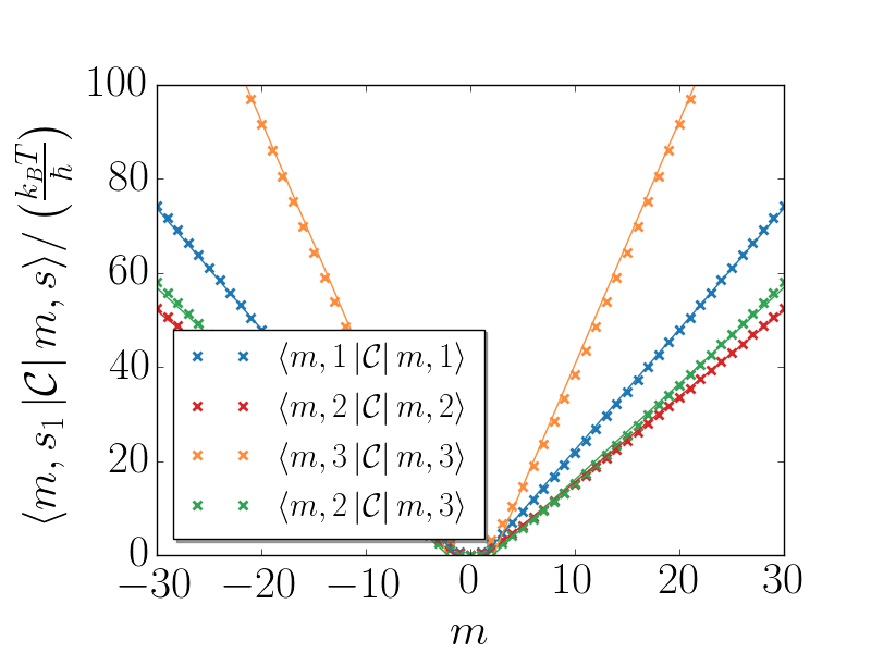
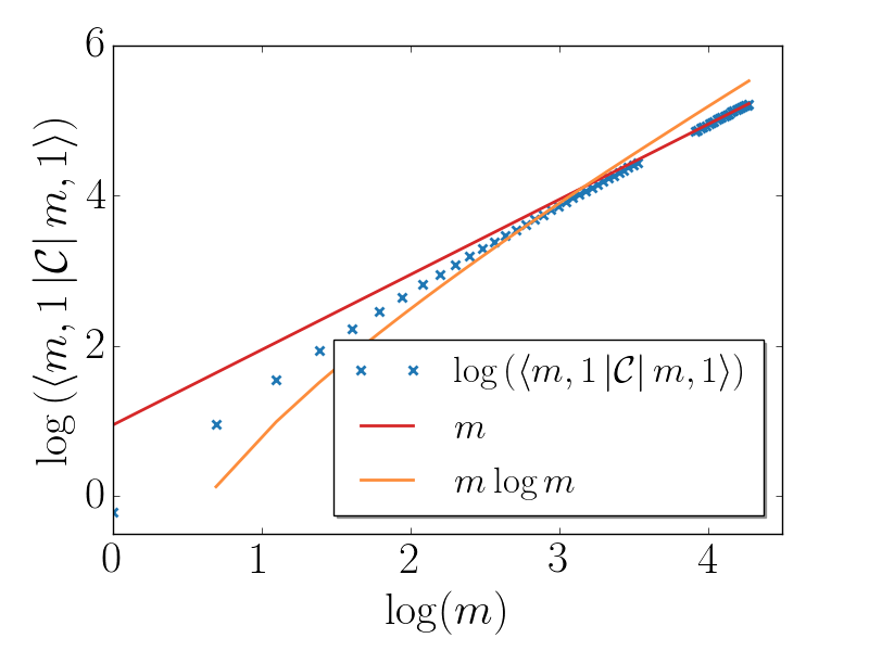
Figure 2: Upper panel: Angular momentum dependence of the matrix elements of the collision operator $\left\langle m,s\left|{\cal C}\right|m,s^{\prime}\right\rangle$ where $s=1\cdots 3$ refers to the collinear eigenmodes of Eq.9. In the text we discuss, for simplicity, only $\left\langle m\left|{\cal C}\right|m\right\rangle\equiv\left\langle m,1\left|{\cal C}\right|m,1\right\rangle$. Lower panel: log-log plot of the matrix element to demonstrate that we can distinguish the $\left|m\right|$-dependence from, e.g. $\left|m\right|\log\left|m\right|$.

The implication of the $\left|m\right|$-dependence of $\tau_{m}^{-1}$ becomes evident if we consider the scattering between two distinct momentum directions. Fourier transformation of $\tau_{m}^{-1}$ yields:

$$\left\langle\theta\left|{\cal C}\right|\theta^{\prime}\right\rangle = -\frac{\ln 2\tau_{L}^{-1}}{\left(2\pi\right)^{2}\sin^{2}\left(\frac{\theta-\theta^{\prime}}{2}\right)}.$$ (13)

Thus, we obtain a slowly-decaying powerlaw $\sim\left(\theta-\theta^{\prime}\right)^{-2}$ for scattering processes away from forward scattering. Using this result for $\left\langle\theta\left|{\cal C}\right|\theta^{\prime}\right\rangle$ we can rewrite the Boltzmann equation in the form Eq. (2) with characteristic time $\tau_{L}$ of Eq. (3) for the Lévy flight. To arrive at Eq. (2) we used that the convolution of the distribution function with $\left\langle\theta\left|{\cal C}\right|\theta^{\prime}\right\rangle$ can be expressed as a fractional derivative

$$\left(\frac{\partial^{2}g\left(\theta\right)}{\partial\theta^{2}}\right)^{1/2}=\frac{\partial}{\partial\theta}\int_{0}^{2\pi}\frac{g\left(\theta^{\prime}\right)}{\tan\left(\frac{\theta-\theta^{\prime}}{2}\right)}d\theta^{\prime},$$ (14)

a special case of the Riesz-Feller derivative $\triangle^{\mu/2}$Samko1993 ; Hermann2014 .

There are some profound implications that this fractional Fokker-Planck formulation immediately reveals. For example, we consider a scenario where we inject a highly directed excitationLedwith2019 . To this end we consider a source term in the Boltzmann equation that causes this excitation:

$$S_{\mathbf{k}\lambda}\left(t\right)=\delta\left(t\right)f_{k}^{\left(0\right)}\left(1-f_{k}^{\left(0\right)}\right)\sum_{m}\delta h_{\lambda m}e^{im\theta}.$$ (15)

We assumed that we will only inject excitations in a window $\pm k_{B}T$ near the Dirac point, hence the factor $f_{k}^{\left(0\right)}\left(1-f_{k}^{\left(0\right)}\right)$. In addition we decomposed the source term into its angular momentum modes. The linearized Boltzmann equation is applicable if $\left|\delta h_{\lambda m}\right|\ll 1$. To describe an excitation that is peaked along an axis given by a certain momentum direction, we use $\delta h_{\lambda,m}=\delta h\lambda^{m}$, which has a $\lambda$-dependence of the $s=1$ mode of Eq. (9). The solution of the fractional Fokker-Planck equation for a homogeneous case $\mathbf{q}=0$ is then given as

$$\psi_{\lambda}\left(\theta,t\right)=\delta h\Theta\left(t\right)\frac{\sinh\left(t/\tau_{L}\right)}{\cosh\left(t/\tau_{L}\right)-\lambda\cos\left(\theta\right)}.$$ (16)

This function is known as wrapped Cauchy distribution with circular variance $1-e^{-t/\tau_{L}}$Levy1939 ; Mardia1999 . $\Theta\left(t\right)$ is the step function. $\psi_{+}\left(\theta,t\right)$ is shown in the upper panel of Fig. 3.

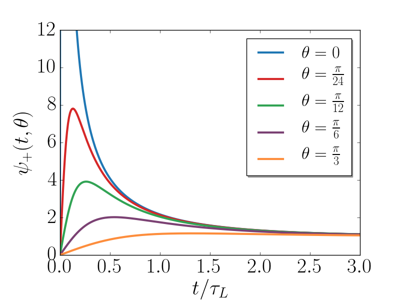
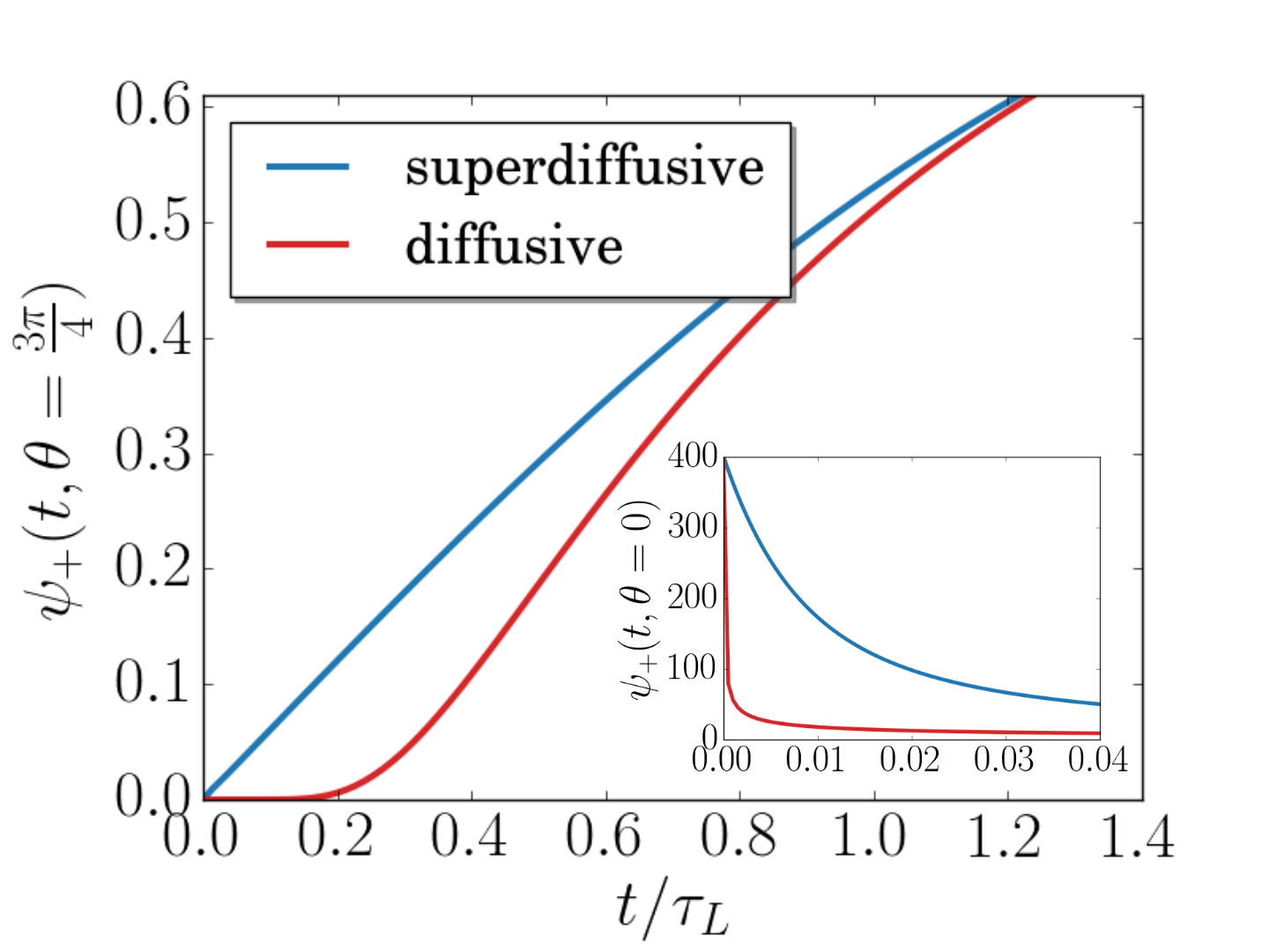
Figure 3: Upper panel: Post-injection distribution function that follows from the fractional Fokker-Planck equation, Eq.2, with external perturbation of Eq.15. Notice the superdiffusive dynamics at short times. Lower panel: Comparison of superdiffusive and diffusive dynamics at short times. At angles away from the peak at $\theta=0$ superdiffusion leads to a faster growth of the distribution function. Inlet: the initial peak at $\theta=0$ decays as $1/t$ for superdiffusion and $1/\sqrt{t}$ for ordinary diffusion. This behavior dominates the heating of the system (see main text).

For $t=0$, $\psi_{\lambda}\left(\theta,t\right)$ corresponds to two delta functions due to particle and hole flows in opposite directions. Let us concentrate on the particle channel $\lambda=+1$. For short times $t\ll\tau_{L}$, the peak in the initial current direction decays as

$$\psi_{+}\left(t,\theta=0\right)\approx\delta h\frac{\tau_{L}}{\pi t},$$ (17)

while the distribution function grows linearly for all non-zero angles:

$$\psi_{+}\left(t,\theta\neq 0\right)\approx\frac{\delta h}{4\pi\sin^{2}\left(\theta/2\right)}\frac{t}{\tau_{L}}.$$ (18)

The same behavior occurs for $\lambda=-1$ if we shift $\theta\rightarrow\theta+\pi$. This behavior in contrast to the one that follows from usual Fokker-Planck diffusion. The latter we obtain for example from collision rates $\tau_{m}^{-1}\sim m^{2}.$ Then the usual spreading of a Gaussian wave package occurs with $\psi_{+}\left(t,\theta=0\right)\propto t^{-1/2}$ and $\psi_{+}\left(t,\theta\neq 0\right)\propto t^{2}$ (lower panel of Fig. 3). While the forward direction of a Levy flight decays more slowly than in usual diffusion, the growth at larger angles is much faster, hence the name superdiffusion.

A tangible implication of this superdiffusive charge motion is the heating of the system after the injection. To this end we determine the time dependence of the entropy density

$$\frac{\partial s\left(t\right)}{\partial t}=4k_{B}\sum_{\lambda}\int_{k}\log\left(\frac{1-f_{\mathbf{k}\lambda}}{f_{\mathbf{k}\lambda}}\right)\frac{\partial f_{\mathbf{k\lambda}}}{\partial t}.$$ (19)

The heat density caused by the injection is given by $\delta q\left(t\right)=T\left(s_{{\rm eq}}-s\left(t\right)\right).$ Inserting the distribution function of Eq. (16) we obtain

$$\frac{\partial s\left(t\right)}{\partial t}=\frac{4\log 2}{9\zeta\left(3\right)}\frac{s_{{\rm eq}}}{\tau_{L}}\frac{\left(\delta h\right)^{2}}{\sinh^{2}\left(t/\tau_{L}\right)},$$ (20)

where $s_{{\rm eq}}$ is the equilibrium entropy density. In order to stay within the regime of linear response, we are confined to $t>\delta h\tau_{L}$. For $t\rightarrow\infty$ one finds $s\rightarrow s_{{\rm eq}},$ and we obtain $s\left(t\right)=s_{{\rm eq}}\left(1-\left(\delta h\right)^{2}\frac{4\log(2)}{9\zeta\left(3\right)}\left(\coth\left(\frac{t}{\tau_{L}}\right)-1\right)\right)$. Thus, initial heating occurs according to

$$\delta q\left(t\right)\propto Ts_{{\rm eq}}\delta h^{2}\frac{\tau_{L}}{t}.$$ (21)

This result is a direct consequence of the superdiffusive behavior, in particular of the slow decay along the forward direction. In case of ordinary diffusion follows $\delta q\left(t\right)\propto t^{-1/2}$ which is much faster (see Fig. 3). The $m$-dependence of $\tau_{m}^{-1}$ that is responsible for the Lévy flight behavior can also be seen in non-local transport coefficients since the conductivity at finite momentum $\mathbf{q}$ couples the different harmonics of the distribution function. As an example we show in the supplementary material the transverse optical conductivity at finite $\mathbf{q}$. Nevertheless, experiments with directed electron beams Wang2019 , which in the past have been used to investigate electron-electron scattering effects Predel2000 , seem to offer a more direct way of testing the short time behavior of Eq. (21).

The occurrence of Lévy flights to describe scattering processes in momentum space is a more general phenomenon and not restricted to graphene at the neutrality point. In two-dimensional Fermi liquids with characteristic rate $\hbar\tau_{FL}^{-1}\sim k_{B}T^{2}/T_{F}$, it holds for $\left|m\right|<M\sim\sqrt{T_{F}/T}$ that $\tau_{m}$${}^{-1}\sim\tau_{FL}^{-1}\frac{m^{p}}{M^{p}}\log\left|m\right|$ with $p=2\left(1+\left(-1\right)^{m}\right)$, while $\tau_{m}^{-1}\sim\tau_{FL}^{-1}$ for $\left|m\right|>M$Gurzhi1996 ; Ledwith2019 . $T_{F}$ is the Fermi temperature. This yields superdiffusive behavior in a wide time window. Another system that also shows $\tau_{m}^{-1}\propto\left|m\right|$ for arbitrarily large $m$ consists of electrons in a random magnetic field, important for the description of composite fermions in the fractional quantum Hall regimeMirlin1997 . Our analysis implies that this system should also undergo a wrapped Cauchy flight in momentum space. Large classes of quantum-critical systems, discussed e.g. in Refs.Hertz1976 ; Moriya1984 ; Millis1993 ; Laughlin2001 ; Millis2002 ; Abanov2003 ; Loehneysen2007 ; DellAnna2007 ; Metlitski2010 ; Schattner2016 ; Damle1997 are governed by long-ranged soft-mode interactions. An analysis of collision processes along the lines discussed here may reveal a non-analytic dependence of the scattering rates on angular momentum quantum number according to $\tau_{m}^{-1}\propto\left|m\right|^{\mu/2}$. This would give rise to a more general class of wrapped Lévy flights, a consequence of the power-law behavior $\left\langle\theta\left|{\cal C}\right|\theta^{\prime}\right\rangle\propto\left|\theta-\theta^{\prime}\right|^{-1-\frac{\mu}{2}}$ near forward scattering. This could occur on the Fermi surface for itinerant quantum critical systems or near a soft momentum in critical bosonic systems. If a fractional Fokker-Planck formulation, along the lines of our Eq. (2), can be derived, it will be significantly easier to draw conclusions about the out-of-equilibrium dynamics of the system such as a focussed injection of collective excitations. Finally we mention that the formulation of the Boltzmann equation presented here can also be used to study the non-local electric and thermal conductivities and viscosities, allowing insight into the diffusive and sound excitations in the hydrodynamic regimeKiselev2019b .

Acknowledgements: We are grateful to Andrey V. Chubukov, Leonid S. Levitov, Dimitrii L. Maslov, and Alexander D. Mirlin for stimulating discussions and to the European Commission’s Horizon 2020 RISE program Hydrotronics for support.

Supplementary material

I Summary of the Simulations shown in Fig.1

Superdiffusion on the Dirac cone can be seen as a random walk of particles, where the step sizes are distributed according to a wrapped Cauchy distribution. This distribution solves the fractional Fokker-Planck equation (2) of the main text (see Chechkin2004 ; Metzler2012 ). The anglular distance on the Dirac cone travelled by an electron during a time interval $\Delta t$ is therefore distributed according to

$$\tilde{\psi}\left(\theta,\Delta t\right)=\frac{\sinh\left(\Delta t/\tau_{L}\right)}{\cosh\left(\Delta t/\tau_{L}\right)-\cos\left(\theta\right)}.$$ (22)

To generate Figs. 1 a) and b) of the main text we created a sequence of random angles $\Delta\theta_{i}$ using the distribution (22). The position of the particle after $N$ steps, i.e. after a time intervall $N\Delta t$, then is

$$\theta_{N}=\sum_{i=0}^{N}\Delta\theta_{i}.$$ (23)

Fig. 4 depicts a wrapped Cauchy random walk with $N=500$ steps.

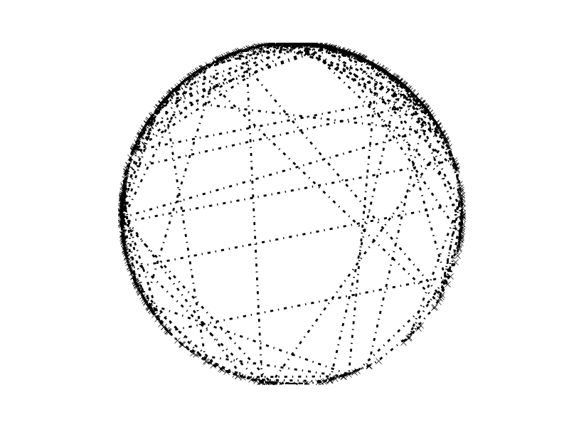
Figure 4: 500 steps of a superdiffusive wrapped Cauchy random walk of an electron on the Dirac cone.

In the case of ordinary diffusion, the step size distribution of Eq. (22) must be replaced by a wrapped normal distribution, which is written in terms of the Jacobi theta function, but can be closely approximated by the van Mises distribution (see e.g. Ref. Kurz2014 ):

$$\tilde{\psi}_{\textrm{normal}}\left(\theta,\Delta t\right)=\frac{e^{\cos\left(\theta\right)/\Delta t}}{2\pi I_{0}\left(1/\Delta t\right)}.$$

Using the described procedure we obtain the wrapped Gaussian random flight shown in Fig. 5.

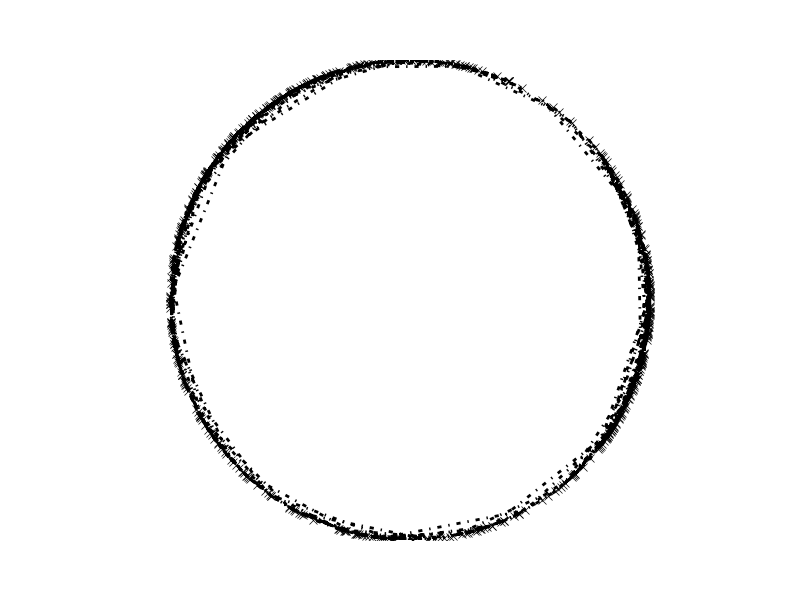
Figure 5: 500 steps of a wrapped Gaussian random walk. The wrapped normal distribution was approximated by the von Mises distribution.

II Collision operator due to electron-electron Coulomb interaction

We briefly summarize the main steps in deriving the collision operator of the Boltzmann equation used in this paper. The collision operator is determined from the larger and smaller self energies on the Keldysh contour. For further details, see Ref. Fritz2008-1 .

The non-interacting part of the Hamiltonian is

$$H_{0}=v\hbar\int_{k}\sum_{\alpha\beta}\psi_{\alpha}^{\dagger}\left(\mathbf{k}\right)\left(\mathbf{k\cdot\sigma}\right)_{\alpha\beta}\psi_{\beta}\left(\mathbf{k}\right)$$ (24)

which is diagonalized by the unitary transformation

$$U_{\mathbf{k}}=\frac{1}{\sqrt{2}}\left(\begin{array}[]{cc}\frac{k_{x}+ik_{y}}{k}&1\\ -\frac{k_{x}+ik_{y}}{k}&1\end{array}\right)$$ (25)

with

$$U_{\mathbf{k}}v\hbar\mathbf{k\cdot\sigma}U_{\mathbf{k}}^{-1}=\left(\begin{array}[]{cc}v\hbar k&0\\ 0&-v\hbar k\end{array}\right).$$ (26)

The eigenvalues of the Hamiltonian are $\pm v\hbar k$. Thus we obtain quasiparticle states for the two bands: $\gamma_{\mathbf{k}}=U_{\mathbf{k}}\psi_{\mathbf{k}}$ with

$$H_{0}=v\hbar\int_{\mathbf{k}}\sum_{\lambda=\pm}\lambda k\gamma_{\mathbf{k},\lambda}^{\dagger}\gamma_{\mathbf{k},\lambda}.$$ (27)

The electron-electron Coulomb interaction is

$$H_{{\rm int}}=\frac{1}{2}\int_{k,k^{\prime},q}\sum_{\alpha\beta}V\left(\mathbf{q}\right)\psi_{\alpha}^{\dagger}\left(\mathbf{k+q},t\right)\psi_{\beta}^{\dagger}\left(\mathbf{k}^{\prime}-\mathbf{q},t\right)\psi_{\beta}\left(\mathbf{k}^{\prime},t\right)\psi_{\alpha}\left(\mathbf{k,}t\right)$$ (28)

with $V\left(q\right)=\frac{e^{2}}{2\pi\varepsilon\left|\mathbf{q}\right|}$. Transforming the interaction into the band, or helical representation, which takes into account the locking between momentum and pseudo-spin that originates from the two sub-lattice structure of graphene. It follows

$$H_{{\rm int}}=\frac{1}{2}\int_{k,k^{\prime},q}\sum_{\alpha\beta}T_{\lambda\mu\mu^{\prime}\lambda^{\prime}}\left(\mathbf{k,k}^{\prime},\mathbf{q}\right)\gamma_{\lambda^{\prime}}^{\dagger}\left(\mathbf{k+q},t\right)\gamma_{\mu}^{\dagger}\left(\mathbf{k}^{\prime}-\mathbf{q},t\right)\gamma_{\mu^{\prime}}\left(\mathbf{k}^{\prime},t\right)\gamma_{\lambda}\left(\mathbf{k,}t\right)$$ (29)

where

$$T_{\lambda\mu\mu^{\prime}\lambda^{\prime}}\left(\mathbf{k,k}^{\prime},\mathbf{q}\right)=V\left(q\right)\left(U_{\mathbf{k+q}}U_{\mathbf{k}}^{-1}\right)_{\lambda^{\prime}\lambda}\left(U_{\mathbf{k}^{\prime}-\mathbf{q}}U_{\mathbf{k}^{\prime}}^{-1}\right)_{\mu\mu^{\prime}}.$$ (30)

Within second order perturbation theory it holds for the self energies for occupied and unoccupied states, respectively.

$$\Sigma{}_{\lambda}^{\gtrless}\left(\mathbf{k,}\omega\right) = N\sum_{\mu\mu^{\prime}\lambda^{\prime}}\int\frac{d^{2}qd^{2}k^{\prime}d\omega_{1}d\omega_{2}}{\left(2\pi\right)^{6}}\left|T_{\lambda\mu\mu^{\prime}\lambda^{\prime}}\left(\mathbf{k,k}^{\prime},\mathbf{q}\right)\right|^{2}$$ (31)

$$\times G_{\lambda^{\prime}}^{\gtrless}\left(\mathbf{k+q,}\omega_{1}\right)G_{\mu}^{\gtrless}\left(\mathbf{k}^{\prime}-\mathbf{q,}\omega_{2}\right)G_{\mu^{\prime}}^{\lessgtr}\left(\mathbf{k}^{\prime}\mathbf{,}\omega_{1}+\omega_{2}-\omega\right)$$

$$- \sum_{\mu\mu^{\prime}\lambda^{\prime}}\int\frac{d^{2}qd^{2}k^{\prime}}{\left(2\pi\right)^{4}}\int\frac{d\omega_{1}d\omega_{2}}{\left(2\pi\right)^{2}}T_{\lambda\lambda^{\prime}\mu^{\prime}\mu}\left(\mathbf{k,k}^{\prime},\mathbf{k}^{\prime}-\mathbf{q-k}\right)T_{\lambda\mu\mu^{\prime}\lambda^{\prime}}\left(\mathbf{k,k}^{\prime},\mathbf{q}\right)^{\ast}$$

$$\times G_{\lambda^{\prime}}^{\gtrless}\left(\mathbf{k+q,}\omega_{1}\right)G_{\mu}^{\gtrless}\left(\mathbf{k}^{\prime}-\mathbf{q,}\omega_{2}\right)G_{\mu^{\prime}}^{\lessgtr}\left(\mathbf{k}^{\prime}\mathbf{,}\omega_{1}+\omega_{2}-\omega\right).$$

$N$ combines the valley and spin degrees of freedom and takes the value $N=4$. Next we use the fact that within a quasiparticle description the upper and lower propagators are expressed in terms of the distribution functions $f_{\lambda}\left(\mathbf{k},\mathbf{r},t\right)$ as

$$G_{\lambda}^{>}\left(\mathbf{k,}\mathbf{r},\omega,t\right) = -i2\pi\delta\left(\omega-\varepsilon_{\lambda}\left(\mathbf{k}\right)\right)\left(1-f_{\lambda}\left(\mathbf{k},\mathbf{r},t\right)\right)$$

$$G_{\lambda}^{<}\left(\mathbf{k,}\mathbf{r},\omega,t\right) = i2\pi\delta\left(\omega-\varepsilon_{\lambda}\left(\mathbf{k}\right)\right)f_{\lambda}\left(\mathbf{k},\mathbf{r},t\right)$$ (32)

As usual, $\mathbf{k}$ and $\omega$ stand for the Fourier-transformed variables of the relative coordinates and times while $\mathbf{r}$ and $t$ stand for the center of gravity or mean time.

The collision operator can now we determined from the self energies $\Sigma^{<}$ and $\Sigma^{>}$:

$${\cal C}_{\lambda}\left(\mathbf{k}\right)=-i\Sigma_{\lambda}^{<}\left(\mathbf{k,}\varepsilon_{\lambda}\left(\mathbf{k}\right)\right)\left(1-f_{\lambda}\left(\mathbf{k}\right)\right)-i\Sigma_{\lambda}^{>}\left(\mathbf{k,}\varepsilon_{\lambda}\left(\mathbf{k}\right)\right)f_{\lambda}\left(\mathbf{k}\right).$$ (33)

For simplicity we only keep the momentum $\mathbf{k}$ and band index $\lambda$. Inserting $G^{>}$ and $G^{<}$ into the self energies yields with the linearization Eq.(6) of the main paper the result for the collision operator given in Eq.(8) of the main paper. The matrix elements $\gamma_{\mathbf{k},\mathbf{k}^{\prime},\mathbf{q}}^{\left(1,2\right)}$ of that equation are given as:

$$\gamma_{1}\left(\mathbf{k,k}^{\prime},\mathbf{q}\right) = \left(N-1\right)\left|T_{A}\left(\mathbf{k,k}^{\prime},\mathbf{q}\right)\right|^{2}+\frac{1}{2}\left|T_{A}\left(\mathbf{k,k}^{\prime},\mathbf{k}^{\prime}-\mathbf{q-k}\right)-T_{A}\left(\mathbf{k,k}^{\prime},\mathbf{q}\right)\right|^{2}$$

$$-\left|T_{A}\left(\mathbf{k,k}^{\prime},\mathbf{k}^{\prime}-\mathbf{q-k}\right)\right|^{2}$$

$$\gamma_{2}\left(\mathbf{k,k}^{\prime},\mathbf{q}\right) = \left(N-1\right)\left|T_{B}\left(\mathbf{k,\mathbf{k}^{\prime}},\mathbf{\mathbf{k}^{\prime}-k-\mathbf{q}}\right)\right|^{2}+\left(N-1\right)\left|T_{A}\left(\mathbf{k,\mathbf{k}^{\prime}},\mathbf{q}\right)\right|^{2}$$ (34)

$$+\left|T_{A}\left(\mathbf{k,\mathbf{k}^{\prime}},\mathbf{q}\right)-T_{B}\left(\mathbf{k,\mathbf{k}^{\prime}},\mathbf{\mathbf{k}^{\prime}-\mathbf{q}}\mathbf{-k}\right)\right|^{2},$$

with

$$T_{A}\left(\mathbf{k,k}^{\prime},\mathbf{q}\right) = T_{++++}\left(\mathbf{k,k}^{\prime},\mathbf{q}\right)=T_{----}\left(\mathbf{k,k}^{\prime},\mathbf{q}\right)$$

$$= T_{+--+}\left(\mathbf{k,k}^{\prime},\mathbf{q}\right)=T_{-++-}\left(\mathbf{k,k}^{\prime},\mathbf{q}\right)$$

$$= \frac{V\left(q\right)}{4}\left(1+\frac{\left(K+Q\right)K^{\ast}}{\left|\mathbf{k+q}\right|k}\right)\left(1+\frac{\left(K^{\prime}-Q\right)K^{\prime\ast}}{\left|\mathbf{k}^{\prime}\mathbf{-q}\right|k^{\prime}}\right)$$

and

$$T_{B}\left(\mathbf{k,k}^{\prime},\mathbf{q}\right) = T_{++--}\left(\mathbf{k,k}^{\prime},\mathbf{q}\right)=T_{--++}\left(\mathbf{k,k}^{\prime},\mathbf{q}\right)$$ (35)

$$= \frac{V\left(q\right)}{4}\left(1-\frac{\left(K+Q\right)K^{\ast}}{\left|\mathbf{k+q}\right|k}\right)\left(1-\frac{\left(K^{\prime}-Q\right)K^{\prime\ast}}{\left|\mathbf{k}^{\prime}\mathbf{-q}\right|k^{\prime}}\right)$$

Upper-case letters like $K=k_{x}+ik_{y}$ etc. combine the two components of the momentum onto a complex variable.

From the same unitary transformation also follows that

$$U_{\mathbf{k}}\mathbf{\sigma}U_{\mathbf{k}}^{-1}=\frac{\mathbf{k}}{k}\sigma_{z}-\frac{\mathbf{k\times e}_{z}}{k}\sigma_{y}.$$ (36)

This can be used to analyze the current

$$\mathbf{j=}ev\int_{\mathbf{k}}\psi^{\dagger}\left(\mathbf{k}\right)\mathbf{\sigma}\psi\left(\mathbf{k}\right)$$ (37)

of Dirac particles which consists of intra- and inter-band contributions:

$$\mathbf{j=j}_{\mathrm{intra}}+\mathbf{j}_{\mathrm{inter}}.$$ (38)

The two terms are given as

$$\mathbf{j}_{\mathrm{intra}} = ev\int_{\mathbf{k}}\sum_{\lambda=\pm}\frac{\lambda\mathbf{k}}{k}\gamma_{\mathbf{k},\lambda}^{\dagger}\gamma_{\mathbf{k},\lambda}$$

$$\mathbf{j}_{\mathrm{inter}} = iev\int_{\mathbf{k}}\frac{\mathbf{k\times e}_{z}}{k}\left(\gamma_{\mathbf{k},+}^{\dagger}\gamma_{\mathbf{k},-}-\gamma_{\mathbf{k},-}^{\dagger}\gamma_{\mathbf{k},+}\right).$$ (39)

Thus, the velocity used in our Eq. (4) of the main paper is precisely the expression $\mathbf{v}_{\mathbf{k}\lambda}=v\frac{\lambda\mathbf{k}}{k}$ of the intraband current $\mathbf{j}_{\mathrm{intra}}$. Spin-momentum locking is included naturally, if one goes to the helical states of the upper and lower Dirac cone. The hydrodynamic response is governed by strong collisions of intraband excitations.

III Identification of the collinear modes at finite angular momentum

In this section we determine the zero modes of the collision operator of Eq.(8) if we confine ourselves to collinear collision processes. To this end we need to find under what conditions the two expressions

$$A_{\mathbf{k},\mathbf{k}^{\prime},\mathbf{q},\lambda}^{\left(1\right)} = \psi_{\mathbf{k}+\mathbf{q}\lambda}+\psi_{\mathbf{k}^{\prime}-\mathbf{q}\lambda}-\psi_{\mathbf{k}^{\prime}\lambda}-\psi_{\mathbf{k}\lambda}$$

$$A_{\mathbf{k},\mathbf{k}^{\prime},\mathbf{q},\lambda}^{\left(2\right)} = \psi_{\mathbf{k}+\mathbf{q}\lambda}-\psi_{-\mathbf{k}^{\prime}+\mathbf{q}\bar{\lambda}}+\psi_{-\mathbf{k}^{\prime}\bar{\lambda}}-\psi_{\mathbf{k}\lambda},$$ (40)

that occur in Eq.(8), vanish. Here we have to include the additional constrain

$$\left|\mathbf{k}+\mathbf{q}\right|+\left|\mathbf{k}^{\prime}-\mathbf{q}\right|=\left|\mathbf{k}\right|+\left|\mathbf{k}^{\prime}\right|$$ (41)

that follows from energy conservation.

By collinear modes we mean that all involved momenta are either parallel or antiparallel. As discussed in Ref.Fritz2008-1 we consider such zero modes of collinear processes because all other processes are suppressed by $1/\log\left(1/\alpha\right)$ where $\alpha$ is the fine-structure constant. Of course, the analysis allows for scattering processes that are not collinear; the issue is merely that distribution functions that become zero modes for collinear scattering are enhanced relative to those that are no such zero modes. Finally we comment that the main conclusion of our paper, namely that the scattering rate depends on angular momentum like $\tau_{m}^{-1}\propto k_{B}T\left|m\right|$, is unchanged if we go beyond the collinear mode regime.

One immediately finds that $A^{\left(1\right)}=B^{\left(1\right)}=0$ subject to Eq.41 is obeyed by $\psi_{\mathbf{k},\lambda}=1$, $\psi_{\mathbf{k},\lambda}=\mathbf{k}$, and $\psi_{\mathbf{k},\lambda}=\lambda\left|\mathbf{k}\right|$, regardless of whether we confine ourselves to collinear modes. These modes correspond to the conservation of charge, momentum, and energy, respectively. In addition to these modes one also finds $\psi_{\mathbf{k},\lambda}=\lambda$ is a zero mode. It corresponds to the fact that second order perturbation theory does not relax a charge imbalance between the upper and lower Dirac cone.

Next we consider distribution functions

$$\psi_{\mathbf{k},\lambda}=a_{\lambda,m}\left(k\right)e^{im\theta_{\mathbf{k}}},$$ (42)

where $k=\left|\mathbf{k}\right|$ is the magnitude of the momentum and $\theta_{\mathbf{k}}$ its polar angle: $\mathbf{k}=k\left(\cos\theta_{\mathbf{k}},\sin\theta_{\mathbf{k}}\right)$. Collinear scattering corresponds to

$$\mathbf{\theta_{\mathbf{k}}=\theta_{\mathbf{k}^{\prime}}+s_{1}\pi=\theta_{\mathbf{k}+\mathbf{q}}+s_{2}\pi=\theta_{\mathbf{k}^{\prime}-\mathbf{q}}+s_{3}\pi},$$ (43)

where even or odd $s_{i}$ correspond to parallel and antiparallel momenta relative to $\mathbf{k}$. We first show that all $s_{i}$ are even due to energy conservation. To this end we assume without restriction that $\mathbf{k}=\left(k,0\right)$ with $k>0$. Then $\mathbf{k}^{\prime}=u\left(k,0\right)$ and $\mathbf{q}=w\left(k,0\right)$, where we do not assume that $u$ and $w$ are positive. Energy conservation now implies

$$1+\left|u\right|=\left|1+w\right|+\left|u-w\right|.$$ (44)

We need to fulfill this condition for an extended set of variables, not just for an isolated point in momentum space. This implies that $1+w>0$ so we can cancel the “$1$” on both sides. Then, to be able to cancel $w$ it must hold that $u>w$, which in turn implies $u>0$ to cancel $u$. Thus, we find that the momenta $\mathbf{k}^{\prime}$, $\mathbf{k}+\mathbf{q}$, and $\mathbf{k}^{\prime}-\mathbf{q}$ point in the same direction as $\mathbf{k}$ even though $\mathbf{q}$ is allowed to point in the opposite direction. It follows that we can assume without restriction that

$$\mathbf{\theta_{\mathbf{k}}=\theta_{\mathbf{k}^{\prime}}=\theta_{\mathbf{k}+\mathbf{q}}=\theta_{\mathbf{k}^{\prime}-\mathbf{q}}}.$$ (45)

If we use that $e^{im\theta_{-\mathbf{p}}}=\left(-1\right)^{m}e^{im\theta_{\mathbf{p}}}$we obtain

$$A_{\mathbf{k},\mathbf{k}^{\prime},\mathbf{q},\lambda}^{\left(1\right)} = \left(a_{\lambda,m}\left(\left|\mathbf{k}+\mathbf{q}\right|\right)+a_{\lambda,m}\left(\left|\mathbf{k}^{\prime}-\mathbf{q}\right|\right)-a_{\lambda,m}\left(k^{\prime}\right)-a_{\lambda,m}\left(k\right)\right)e^{im\theta_{\mathbf{k}}}$$

$$A_{\mathbf{k},\mathbf{k}^{\prime},\mathbf{q},\lambda}^{\left(2\right)} = \left(a_{\lambda,m}\left(\left|\mathbf{k}+\mathbf{q}\right|\right)-\left(-1\right)^{m}a_{\bar{\lambda},m}\left(\left|\mathbf{k}^{\prime}-\mathbf{q}\right|\right)+\left(-1\right)^{m}a_{\bar{\lambda},m}\left(k^{\prime}\right)-a_{\lambda,m}\left(k\right)\right)e^{im\theta_{\mathbf{k}}}.$$ (46)

It is now easy so find that there are the following solutions that yield $A^{\left(1\right)}=B^{\left(1\right)}=0$ subject to Eq.41:

$$a_{\lambda,m}\left(k\right) = 1$$

$$a_{\lambda,m}\left(k\right) = \lambda.$$ (47)

In addition one finds $a_{\lambda,m}\left(k\right)=\lambda\left|\mathbf{k}\right|$ if $m$ is even and $a_{\lambda,m}\left(k\right)=\left|\mathbf{k}\right|$ if $m$ is odd.

Thus, we can write that the following modes are zero modes in the collinear scattering limit

$$\psi_{\mathbf{k},\lambda}=\lambda^{m}e^{im\theta_{\mathbf{k}}}\left(1,\lambda,\lambda\left|\mathbf{k}\right|\right)$$ (48)

which is Eq.(9) of the main paper.

IV Superdiffusion and non-local transport

The Fokker-Planck equation (2) of the main text

$$\left(\partial_{t}+\mathbf{v}_{\mathbf{k}\lambda}\cdot\nabla_{\mathbf{x}}-\tau_{L}^{-1}\left(\frac{\partial^{2}}{\partial\theta^{2}}\right)^{1/2}\right)f_{\mathbf{k}\lambda}=S_{\mathbf{k}\lambda}$$ (49)

can be used to calculate the response of graphene electrons to an external perturbation, such as for example an electric field. In this case the force term is given by

$$S_{\mathbf{k}\lambda}=-e\mathbf{E}\left(\mathbf{q},\omega\right)\cdot\frac{\partial f_{\mathbf{k}\lambda}}{\partial\mathbf{k}},$$

where $\mathbf{E\left(\mathbf{q},\omega\right)}=E_{0}e^{i\left(\mathbf{q}\cdot\mathbf{x}-\omega t\right)}\mathbf{e}_{x}$ is the electric field. To first order in the electric field it is

$$S_{\mathbf{k}\lambda}=-eE_{0}e^{i\mathbf{q}\cdot\mathbf{x}}\cos\theta\left(\lambda\hbar v\beta\right)f_{k}^{\left(0\right)}\left(1-f_{k}^{\left(0\right)}\right).$$

We perform a Fourier transform $t\rightarrow\omega$, $\mathbf{x}\rightarrow\mathbf{q}$ and project the equation (49) onto the collinear zero modes (48) using the scalar product $\Braket{\phi}{\chi}=\sum_{\lambda}\int\frac{d^{2}k}{\left(2\pi\right)^{2}}\phi_{\bm{k},\lambda}\chi_{\bm{k},\lambda}$. The result is a simplified version of the Boltzmann equation:

$$-i\omega\delta_{m,m^{\prime}}+\frac{1}{2}ivq\left(e^{-i\vartheta_{\bm{q}}}\delta_{m,m^{\prime}+1}+e^{i\vartheta_{\bm{q}}}\delta_{m,m^{\prime}-1}\right)+\frac{1}{\tau_{L}\left|m\right|}=-\frac{1}{2}eE_{0}v\beta\delta_{\left|m\right|,1},$$ (50)

where $m$ labels the angular harmonic of the collinear zero mode and $\vartheta_{\bm{q}}$ is the angle of the wave vector $\mathbf{q}$ with respect to the $x$-axis. This equation is exact in the limit of a small coupling constant $\alpha$, where collinear events dominate the electron-electron scattering Fritz2008-1 . Notice, that the electric field only couples to angular harmonics with $\left|m\right|=1$, however for a spatially inhomogeneous field with $q\neq 0$, the second right hand side term of Eq. (50) couples all angular harmonics. Therefore, information on the $m$-dependence of the scattering times can be extracted from the non-local (i.e. $\mathbf{q}$-dependent) electric conductivity $\sigma_{\alpha\beta}\left(\mathbf{q},\omega\right)$, which is defined through

$$j_{\alpha}\left(\mathbf{q},\omega\right)=\sigma_{\alpha\beta}\left(\mathbf{q},\omega\right)E\left(\mathbf{q},\omega\right).$$

The conductivity tensor $\sigma_{\alpha\beta}\left(\mathbf{q},\omega\right)$ can be decomposed into longitudinal and transverse parts according to

$$\sigma_{\alpha\beta}=\frac{q_{\alpha}q_{\beta}}{q^{2}}\sigma_{\parallel}\left(\omega,q\right)+\left(\delta_{\alpha\beta}-\frac{q_{\alpha}q_{\beta}}{q^{2}}\right)\sigma_{\bot}\left(\omega,q\right),$$

where $\sigma_{\parallel/\bot}\left(\omega,q\right)$ only depend on the magnitude of $\mathbf{q}$. Fig 6 shows the influence of the $m$-dependence of the scattering time $\tau_{m}$ on the real part of the transverse conductivity $\sigma_{\bot}\left(\omega,q\right)$. We conclude that the non-local conductivity, playing an important role in experiments on surface acoustic waves Wixforth1986 ; Simon1996 , provides a possibility to detect the peculiar dependence of the scattering times $\tau_{m}$ on $m$, and to confirm the Lévy flight behavior predicted in the main text.

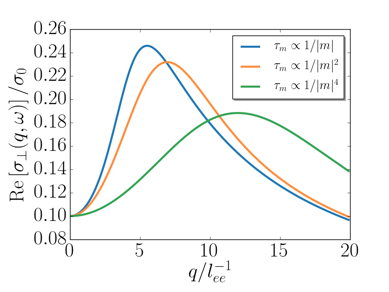
Figure 6: Real part of the transverse conductivity $\sigma_{\bot}\left(\omega,q\right)$ for different dependecies of the scattering times $\tau_{m}$ on $m$. This result was obtain by solving Eq. (50) numerically.

For completeness, we mention that the Boltzmann equation (50) can be solved exactly, and the expressions for the non-local conductivities can be written down in closed form EK2019 :

$$\sigma_{\parallel}\left(q,\omega\right) = \frac{\sigma_{0}}{1+i\tau_{1}\omega-\frac{1}{4}v^{2}\tau_{1}q^{2}\left(\frac{2i}{\omega}-\frac{1}{M\left(q,\omega\right)+i\omega}\right)},$$

$$\sigma_{\bot}\left(q,\omega\right) = \frac{\sigma_{0}}{1+i\tau_{1}\omega+\frac{\frac{1}{4}v^{2}\tau_{1}q^{2}}{M\left(q,\omega\right)+i\omega}}.$$ (51)

Here, $\sigma_{0}=N\frac{e^{2}\log\left(2\right)\tau_{\sigma,1}}{2\pi\beta\hbar^{2}}$ is the quantum critical conductivity calculated in Ref. Fritz2008-1 and $M\left(q,\omega\right)$ is the memory function summerizing the effects of higher angular harmonics:

$$M\left(q,\omega\right)=\tau_{2}^{-1}+\frac{1}{2}vq\frac{\textrm{I}_{3+i\omega\tau_{L}}\left(\tau_{L}vq\right)}{\textrm{I}_{2+i\omega\tau_{L}}\left(\tau_{L}vq\right)},$$

where $I_{\nu}\left(z\right)$ is the modified Bessel function.

References

(1)S. Chandrasekhar, Stochastic Problems
in Physics and Astronomy, Rev. Mod. Phys. 15, 1 (1943).
(2)M. N. Rosenbluth, W. M. MacDonald, and D.
L. Judd, Fokker-Planck Equation for an Inverse-Square Force,
Phys. Rev. 107 1 (1957).
(3)D. F. Chernoff and M. D. Weinberg, Evolution
of globular clusters in the Galaxy, Astrophysical Journal 351,121
(1990).
(5)J. A. Hertz, Quantum critical phenomena,
Phys. Rev. B 14, 1165 (1976).
(6)T. Moriya, Spin Fluctuations in Itinerant
Electron Magnetism, Springer Series in Solid-State Science 52, Springer,
Berlin-Heidelberg (1984).
(7)A. J. Millis, Effect of a nonzero temperature
on quantum critical points in itinerant fermion systems, Phys. Rev.
B 48, 7183 (1993).
(8)R. B. Laughlin, G. G. Lonzarich, P. Monthoux,
and D. Pines, The Quantum Criticality Conundrum, Adv. Phys.
50, 361 (2001).
(9)A. J. Millis, A. J. Schofield, G. G. Lonzarich,
and S. A. Grigera, Metamagnetic Quantum Criticality, Phys.
Rev. Lett. 88, 217204 (2002).
(10)Ar. Abanov, A. V. Chubukov, and J. Schmalian,
Quantum-critical theory of the spin-fermion model and its application
to cuprates: Normal state analysis, Adv. Phys. 52, 119 (2003).
(11)H. v. Löhneysen, A. Rosch, M. Vojta, and
P. Wölfle, Fermi-liquid instabilities at magnetic quantum phase
transitions, Rev. Mod. Phys. 79, 1015 (2007).
(12)L. Dell’Anna and W. Metzner,
Electrical Resistivity near Pomeranchuk Instability in Two Dimensions,
Phys. Rev. Lett. 98, 136402 (2007).
(13)M. A. Metlitski and S. Sachdev, Quantum phase
transitions of metals in two spatial dimensions. I. Ising-nematic
order, Phys. Rev. B 82, 075127 (2010).
(14)Y. Schattner, S. Lederer, S. A. Kivelson,
and E. Berg, Ising Nematic Quantum Critical Point in a Metal:
A Monte Carlo Study, Phys. Rev. X 6, 031028 (2016).
(15)K. Damle and S. Sachdev, Nonzero-temperature
transport near quantum critical points, Phys. Rev. B 56,
8714 (1997).
(16)Daniel E. Sheehy and Jörg Schmalian, Quantum
Critical Scaling in Graphene, Phys. Rev. Lett. 99, 226803 (2007).
(17)R. N. Gurzhi, A. N. Kalinenko, and A. I. Kopeliovich
Phys. Rev. Lett. 74, 3872 (1995).
(19)D. L. Maslov, V. I. Yudson, and A. V. Chubukov,
Phys. Rev. Lett. 106, 106403 (2011).
(20)H. K. Pal, V. I. Yudson, and D. L. Maslov, Resistivity
of non-Galileian invariant Fermi- and Non-Fermi liquids, Lithuanian
Journal of Physics, 52, 142 (2012).
(21)D. L. Maslov and A. V. Chubukov, Optical response
of correlated electron systems, Rep. Prog. Phys. 80, 026503
(2017).
(22)P. J. Ledwith, H. Guo, L. Levitov, The
Hierarchy of Excitation Lifetimes in Two-Dimensional Fermi Gases,
arXiv:1905.03751.
(23)L. Fritz, J. Schmalian, M. Müller and S. Sachdev,
Quantum critical transport in clean graphene, Phys. Rev. B
78, 085416 (2008).
(24)A. B. Kashuba, Conductivity of defectless
graphene, Phys. Rev. B 78, 085415 (2008).
(25)M. Müller, J. Schmalian and L. Fritz, Graphene:
A Nearly Perfect Fluid, Phys. Rev. Lett. 103, 025301 (2009).
(26)M. Schütt, P. M. Ostrovsky, I. V. Gornyi, and
A. D. Mirlin, Coulomb interaction in graphene: Relaxation rates
and transport, Phys. Rev. B 83, 155441 (2011).
(27)E. I. Kiselev, J. Schmalian, Boundary
conditions of viscous electron flow, Phys. Rev. B 99, 035430
(2019).
(28)P. Lévy, P. Théorie de l’Addition des Variables
Aléatoires Gauthier-Villars, Paris, (1954).
(29)B. Mandelbrot, The Fractal Geometry
of Nature, Freeman, New York, (1977).
(30)W. Feller, An Introduction to Probability
Theory and its Applications, 2nd ed., Vol. 2, Wiley, New York, (1971).
(31)S. G. Samko, A. A. Kilbas and O. I. Marichev,
Fractional Integrals and Derivatives, Theory and Applications,
Gordon and Breach, Amsterdam, (1993).
(32)R. Hermann, Fractional Calculus: An Introduction
for Physicists (2nd ed.). New Jersey: World Scientific Publishing
(2014).
(33)F. Bartumeus, M. G. E. Da Luz, G. M. Viswanathan,
J. Catalan, Animal search strategies: A quantitative random-walk
analysis. Ecology 86, 3078 (2005).
(34)A. M. Reynolds and C. J. Rhodes, The
Lévy flight paradigm: random search patterns and mechanisms, Ecology,
90,, 877 (2009).
(35)R. N. Mantegna and H. E. Stanley, Econophysics:
Scaling and its breakdown in finance. Journal of statistical Physics,
89, 469 (1997).
(36)A. Corral, Universal earthquake-occurrence
jumps, correlations with time, and anomalous diffusion Phys. Rev.
Lett. 97, 178501 (2006).
(37)P. Levy, L’addition des variables
aléatoires définies sur une circonférence, Bulletin de la Societe
mathematique de France, 67, 1 (1939),
(38)Kanti V. Mardia and Peter E. Jupp, Directional
Statistics, Wiley (1999) ISBN 978-0-471-95333-3.
(39)see supplementary material.
(40)P. Gallagher, C.-S. Yang, T. Lyu, F. Tian,
R. Kou, H. Zhang, K. Watanabe, T. Taniguchi, and F. Wang, Quantum-critical
conductivity of the Dirac fluid in graphene, Science 364,
158 (2019).
(41)S. Gattenlöhner, I. V. Gornyi, P. M. Ostrovsky,
B. Trauzettel, A. D. Mirlin, M. Titov, Lévy flights due to
anisotropic disorder in graphene. Phys. Rev. Lett. 117,
046603 (2016).
(42)U. Briskot, I. A. Dmitriev, and A. D. Mirlin,
Relaxation of optically excited carriers in graphene: Anomalous
diffusion and Lévy flights, Phys. Rev. B 89, 075414 (2014).
(43)P. Barthelemy, J. Bertolotti, and D. S. Wiersma,
A Lévy flight for light, Nature 453, 495 (2008).
(44)J. Crossno, J. K. Shi, K. Wang, X. Liu, A. Harzheim,
A. Lucas, S. Sachdev, P. Kim, T. Taniguchi, K. Watanabe, T. A. Ohki,
K. C. Fong, Observation of the Dirac fluid and the breakdown
of the Wiedemann-Franz law in graphene, Science 351, 1058
(2016).
(45)H. Predel, H. Buhmann, L. W. Molenkamp, R. N.
Gurzhi, A. N. Kalinenko, A. I. Kopeliovich, A. V. Yanovsky, Phys.
Rev. B 62, 2057 (2000).
(46)K. Wang, M. M. Elahi, L. Wang, K. M. M. Habib,
T. Taniguchi, K. Watanabe, J. Hone, A. W. Ghosh, G.-H. Lee, P. Kim,
PNAS 116, 6575 (2019).
(47)A. D. Mirlin and P. Wölfle, Composite
fermions in the fractional quantum Hall effect: Transport at finite
wave vector, Phys. Rev. Lett. 78, 371 (1997).
(48)E. I. Kiselev and J. Schmalian, unpublished.Supplementary
material: Lévy flights and hydrodynamic superdiffusion on the Dirac
cone of graphene

References

(1)A. V. Chechkin, V. Y. Gonchar, J. Klafter,
R. Metzler, L. V. Tanatarov, J. Stat. Phys. 115, 1505 (2004).
(2)R. Metzler, A. V. Chechkin, J. Klafter, Levy
Statistics and Anomalous Transport, Computational Complexity, Springer,
2012.
(3)G. Kurz, I. Gilitschenski and U. D. Hanebeck, "Efficient
evaluation of the probability density function of a wrapped normal
distribution" in 2014 Sensor Data Fusion: Trends, Solutions,
Applications (SDF), IEEE (2014).
(4)L. Fritz, J. Schmalian, M. Müller and S. Sachdev,
Quantum critical transport in clean graphene, Phys. Rev. B
78, 085416 (2008).
(5)A. Wixforth, J. P. Kotthaus, and G. Weimann
Phys. Rev. Lett. 56, 2104 (1986).