Enhancing Patch-Based Methods with Inter-frame Connectivity for Denoising Multi-frame Images

Abstract

The 3D block matching (BM3D) method is among the state-of-art methods for denoising images corrupted with additive white Gaussian noise. With the help of a novel inter-frame connectivity strategy, we propose an extension of the BM3D method for the scenario where we have multiple images of the same scene. Our proposed extension outperforms all the existing trivial and non-trivial extensions of patch-based denoising methods for multi-frame images. We can achieve a quality difference of as high as 28% over the next best method without using any additional parameters. Our method can also be easily generalised to other similar existing patch-based methods.

Index Terms—  Multi-frame denoising, non-local patch methods, additive white Gaussian noise

1 Introduction

Denoising images corrupted with Gaussian noise is a classical image processing application, on which tremendous amount of research has been performed. Generalised K-Means clustering (K-SVD) [1], autoencoders [2] and deep neural networks [3] are worth mentioning works in this field. For the past two decades, non-local patch based methods [4, 5, 6, 7] have been among the state-of-art methods for this application. Especially, 3D Block Matching (BM3D) in combination with some non-linear transformations and inverse transformations is a widely used method for denoising images which are corrupted with a variety of noise distributions including Gaussian, Poisson and Poisson-Gaussian mixture types of noise [8, 9, 10, 11]. All the above mentioned research work, however, has been performed on denoising single images. Denoising multi-frame images is a less explored field. Electron microscopy, CT imaging, multi-spectral imaging are some of the fields where we encounter the problem of obtaining one image from multiple noisy images of the same sample/scene. Notable works in the field of multi-frame image denoising include non-local patch-based denoising methods [12, 13], low-rank tensor approximation framework with Laplacian scale mixture [14, 15], Stein’s unbiased risk estimator and linear expansion of threshold combining methods [16, 17], multi-scale sparsity denoising of spectral domain optical coherence tomography images [18], non-local energy functional minimisation approach involving spatio-temporal image patches [19], low-rank tensor modelling based denoising approach [20], combining blind source separation and block matching for denoising CT images [21], and tensor based modeling for denoising multi-frame images corrupted with speckle noise [22].

Three different types of baseline strategies can exist that are relevant in extending patch-based methods for denoising multi-frame images: First, average the noisy images and then denoise the averaged image [12]. The second is a trivial strategy introduced by us: Denoise the individual images and then average the denoised images. Finally, a non-trivial strategy [13]: In the initial stage of patch-based denoising methods, the group of patches that are most similar to a patch are acquired from images other than just the reference image also. Once this group of patches are acquired, a traditional single image denoising approach is performed.

Image ($\sigma_{\mathrm{noise}}$)	BM-1	BM-2	BM-3	BM-M
Bridge (80)	316.95	289.69	345.88	266.16
Bridge (100)	352.16	330.92	394.19	307.50
Bridge (120)	380.81	366.45	440.26	345.19
Peppers (80)	83.15	66.08	91.27	59.20
Peppers (100)	111.16	81.88	115.15	74.15
Peppers (120)	141.97	99.85	139.50	89.64
Lena (80)	82.18	81.11	107.10	71.38
Lena (100)	97.89	99.84	135.53	87.49
Lena (120)	114.43	118.85	160.20	107.48
House (80)	66.67	74.41	96.25	62.60
House (100)	83.59	93.40	123.95	80.53
House (120)	98.37	116.31	152.82	96.62

BM-1	BM-2	BM-3	BM-M
299.72	277.90	340.38	230.99
330.23	315.56	386.17	268.01
354.58	348.86	430.78	304.76
71.68	58.39	87.81	47.51
91.63	70.70	109.38	58.45
112.10	85.39	129.35	69.91
72.41	72.45	102.79	56.41
85.95	88.72	125.81	70.85
96.82	104.29	150.64	84.99
56.79	64.70	88.92	48.14
68.97	80.96	114.43	63.03
77.96	99.01	142.30	75.15

Table 1: MSE values after denoising 5-image (left) and 10-image (right) datasets

Our Contribution In this work, our main contribution is a novel strategy that differs from all the above mentioned strategies at three stages. The first and second differences are at the 3D patch grouping stage and the third difference is at the aggregation stage of acquiring the final denoised image. These ideas enhance the denoising quality of the algorithm significantly. We perform a detailed and comprehensive evaluation of all the above mentioned extensions, specifically for BM3D. Such a detailed study of extensions for multi-frame image denoising is missing for any of the patch-based methods in the existing works.

Paper Structure In Section 2, we introduce the various extensions of BM3D for multi-frame images. In Section 3, we present the denoising results of the experiments performed using various extensions of BM3D. We also perform an analysis on why our proposed extension outperforms the other existing approaches. Finally, in Section 4, we conclude the paper with a summary of our work and some ideas for future research.

Fig. 1: Results after denoising 10-image datasets with $\sigma_{\mathrm{noise}}=80$. Top to bottom: Zoomed Lena and Bridge images. Left to right: Original, noisy, BM3D-M, next best method.

Fig. 2: Results after denoising 10-image datasets with $\sigma_{\mathrm{noise}}=80$. Top to bottom: Zoomed House and Peppers images. Left to right: Original, noisy, BM3D-M, next best method.

2 Modelling of denoising algorithm

2.1 Original BM3D Method

BM3D [5] is a two step method for removing additive white Gaussian noise (AWGN). Each step consists of three sub-steps. In the first sub-step of the first main step, a 3D group is created by finding the most similar patches to a reference patch using L₂ distance. In the second sub-step, a 2D bi-orthogonal spline wavelet transform is applied to this 3D group, followed by a 1D Walsh-Hadamard transform in the third dimension. After a hard thresholding, the 3D group undergoes corresponding 1D and 2D inverse transformations. In the third sub-step, a weighted aggregation of all the denoised pixels at a particular position in the 2D image domain is performed to obtain the final denoised pixel at that particular position. Thus, we have a denoised image after the first step. In the first sub-step of the second step, the grouping is done using the denoised image obtained after the first step. In the second sub-step, a 2D discrete cosine transform followed by a 1D Walsh-Hadamard transform is applied on both 3D groups obtained from the noisy image and the denoised image from the first step. Then a Wiener filter is applied on a combination of both of the above transformed 3D groups. The resulting 3D group is then back transformed. In the third sub-step, the same corresponding strategy as in the first main step gives the final denoised image. Thus, the two main steps primarily only differ at the second sub-step. We refer the reader to the original work [5] for more details on the method. The final denoised image using the weighted aggregation process [6] is described as

$$u^{\textrm{{final}}}({\bm{x}})=\frac{\sum\limits_{P}w_{P}^{\textrm{{wien}}}\sum\limits_{Q\in P(\textrm{P})}\chi_{Q}(\bm{x})u^{\textrm{{wien}}}_{Q,P}(\bm{x})}{\sum\limits_{P}w_{P}^{\textrm{{wien}}}\sum\limits_{Q\in P(\textrm{P})}\chi_{Q}(\bm{x})}.$$ (1)

Here, $\bm{x}$ is a position in the image domain $Q$ and $u^{\textrm{{final}}}$ is the final denoised image. The symbol $u^{\textrm{{wien}}}_{Q,P}(\bm{x})$ denotes the estimation of the value at pixel position $\bm{x}$ belonging to the patch $Q$ obtained after the Wiener filtering of the reference patch $P$. Also, $w_{P}^{\textrm{{wien}}}$ is obtained from the emperical Wiener coefficients of patch $P$, $\mathcal{P}(P)$ is the set of most similar patches to the reference patch $P$, and finally $\chi_{Q}(\bm{x})=1$ if $\bm{x}\in Q$ and 0 otherwise.

2.2 Baseline Extensions Applicable for BM3D

The first extension is a trivial existing one [12]: Average all the noisy frames after aligning them and then denoise the averaged image (BM3D-1). Another trivial extension, proposed by us, is to denoise every single image and then average the aligned denoised images (BM3D-2). A third non-trival existing [13] extension (BM3D-3) would be to first consider a reference image. Then while obtaining a 3D group of similar patches in the first step, an L₂ distance evaluation is performed with patches from all the other images also instead of just those from the reference image. The rest of the algorithm remains the same.

2.3 Our Novel Multi-frame Extension BM3D-M

Let us now describe the final extension which is the main extension proposed by us: For every image, we carry out a grouping using L₂ distance evaluation from patches in all the other images. Thus, we use the same grouping strategy as the one proposed in BM3D-3, but we do this for every image. Then we perform the same filtering process as the original BM3D method, for the 3D groups in every image as a part of the second sub-step of the first step. In the third sub-step, the same aggregation process as in the original BM3D method is carried out on every image. Thus, we have as many denoised images as we have input images. In the first sub-step of the second step, we perform the same grouping strategy as we have in the first sub-step of the first step, but using the denoised images of the first step. In the second sub-step, we implement the same filtering process used in the original BM3D method on 3D groups in every image. Finally, in the third sub-step, we carry out an aggregation at a particular position in image domain, using a weighted aggregation of the denoised pixels obtained in ”all the images” at this particular position.

As mentioned in Section 1, our method differs from the other three strategies in three aspects. First, we do not have a reference image like in BM3D-3, but follow the denoising procedure for all the images. This is done in order to maximise the use of available information. Second, in the detailed study for selection for BM3D parameters [6] and in the original work [5], two parameters control the number of patches in a 3D group: The threshold parameter for L₂ distance and the maximum number of patches. In this work we do not use the former parameter as we have the risk of losing some similar patches in the case of highly noisy images. Finally, to obtain the final denoised image, all the other existing extensions perform the weighted aggregation of pixels from 3D groups in just one image. However, since we denoise every image unlike the other three strategies, we perform the weighted aggregation from denoised 3D groups in all the images. The equation that governs the weighted aggregation to obtain the final denoised image is modified as follows:

$$u^{\textrm{{final}}}({\bm{x}})=\frac{\sum\limits_{\ell}\sum\limits_{P_{\ell}}w_{P_{\ell}}^{\textrm{{wien}}}\sum\limits_{Q\in P(\textrm{P}_{\ell})}\chi_{Q}(\bm{x})u^{\textrm{{wien}}}_{Q,P_{\ell}}(\bm{x})}{\sum\limits_{l}\sum\limits_{P_{\ell}}w_{P_{\ell}}^{\textrm{{wien}}}\sum\limits_{Q\in P(\textrm{P}_{\ell})}\chi_{Q}(\bm{x})}.$$ (2)

In the above equation, we can see the extra summation over all the images denoted by index $\ell$. Reference patches $P_{\ell}$ must be considered from every image $\ell$. The rest of the symbols have the same meaning as described in (1).

3 Experiments and Discussion

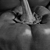
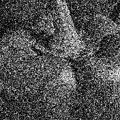
Generally, the various noisy images of the same scene in a multi-frame image denoising problem are first registered before denoising them to obtain the final image. For the registration, one can use a motion estimation method. However, in this work, our aim is to carry out a comprehensive performance study of the extensions for denoising methods. Thus, we assume that all the images are pre-registered so that we can straight away compare the denoising qualities of various algorithms. It is not difficult to combine the denoising strategies proposed by us with state-of-art motion estimation methods. Hence, to satisfy this experimental setting, we have corrupted Lena, House, Peppers and Bridge images with AWGN of standard deviations $\sigma_{\mathrm{noise}}=80,100,120$. Two datasets for each image for each noise standard deviation have been created, one with five realisations of noise and the other with ten realisations of noise.

The threshold parameters for $L_{2}$ distance while forming the 3D groups have been excluded in both the main steps of BM3D for all the four extensions to keep them on an equal footing. This particular step is advantageous to all the extensions for high standard deviation of noise. One can introduce back these parameters in applications where there is less amount of noise ($\sigma_{\mathrm{noise}}<80$). All the other parameters have been chosen according to the detailed study of parameter selection for BM3D in [6]. It also has to be mentioned that, in the results we showcase shortly, we present the mean squared error (MSE) value for BM3D-3 which is the best of the 5/10 denoised images obtained when every image is selected as the reference frame.

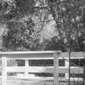
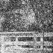
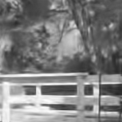
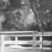
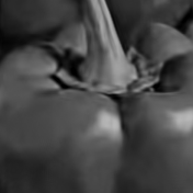
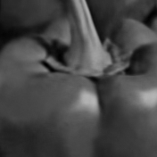
From Table 1 and Figures 1 and 2, we can observe that BM3D-M outperforms all other methods significantly, in terms of both MSE and visually. The images obtained using BM3D-M in particular, appear sharper. Moreover, for the Lena 10-image dataset and $\sigma_{\mathrm{noise}}=80$, the next best method other than BM3D-M is worse by 28%. Thus, BM3D-M has the capability of producing significantly better results than the other algorithms. We attribute these results to the crucial differences in the modelling: inter-frame connectivity strategy in both main steps of BM3D to acquire 3D groups and a weighted aggregation that connects all the frames instead of just one frame.

It is not clear if the BM3D-1 or the BM3D-2 method is better. This is because BM3D-1 does not retain the same explicit noise model that was introduced in the original image after averaging the noisy images and BM3D-2 does not have enough signal in each of the input images in each dataset. Also, we would generally expect the non-trivial BM3D-3 method to perform better than the BM3D-1 and BM3D-2 methods. The three algorithms other than BM3D-3 perform some sort of averaging while BM3D-3 does not. It simply does not make full use of the information available in all the images. This explains its surprisingly inferior performance.

Experiments on an Intel(R) Core(TM) i7-6700 CPU @3.4 GHz using OpenMP indicates that BM3D-M takes 11 times more time than single channel BM3D for the 5-image $256\times 256$ sized House dataset. Also, an ANSI C code combined with a CUDA implementation of BM3D-M on an NVIDIA Quadro P5000 architecture takes 2.7 seconds.

4 Conclusions and Outlook

We have performed the first comprehensive study of extensions for non-local patch-based methods like BM3D for denoising multi-frame image datasets. Our proposed extension which uses novel inter-frame patch and pixel connectivity strategies, gives significantly better results than all the other existing trivial and non-trivial extensions. This improvement of the denoising performance is achieved without using any additional parameters. The new ideas we introduce can also be applied to other similar patch-based methods like BM3D.

In the future, we plan to combine BM3D-M with state-of-art motion registration algorithms and also study the error incurred due to false registration of pixels. We will also study the performance of BM3D-M when the images are corrupted with noise of different standard deviations. Finally, we would apply the algorithm to multi-frame bio-physical image datasets obtained from electron microscopes.

Acknowledgements. J.W. has received funding from the European Research Council (ERC) under the European Union’s Horizon 2020 research and innovation programme (grant agreement no. 741215, ERC Advanced Grant INCOVID).

References

- [1] M. Elad and M. Aharon, “Image denoising via sparse and redundant representations over learned dictionaries,” IEEE Transactions on Image Processing, vol. 15, no. 12, pp. 3736–3745, Dec. 2006.
- [2] P. Vincent, H. Larochelle, I. Lajoie, Y. Bengio, and P.A. Manzagol, “Stacked denoising autoencoders: Learning useful representations in a deep network with a local denoising criterion,” Journal of Machine Learning Research, vol. 11, pp. 3371–3408, Dec. 2010.
- [3] J. Xie, L. Xu, and E. Chen, “Image denoising and inpainting with deep neural networks,” in Proceedings of the 25th International Conference on Neural Information Processing Systems, USA, Dec. 2012, vol. 1 of NIPS’12, pp. 341–349, Curran Associates Inc.
- [4] A. Buades, B. Coll, and J.-M. Morel, “A non-local algorithm for image denoising,” in Proc. 2005 IEEE Computer Society Conference on Computer Vision and Pattern Recognition, San Diego, CA, June 2005, vol. 2, pp. 60–65, IEEE Computer Society Press.
- [5] K. Dabov, A. Foi, V. Katkovnik, and K. Egiazarian, “Image denoising by sparse 3D transform-domain collaborative filtering,” IEEE Transactions on Image Processing, vol. 16, no. 8, pp. 2080–2095, Aug. 2007.
- [6] M. Lebrun, “An analysis and implementation of the BM3D image denoising method,” Image Processing On Line, Aug. 2012.
- [7] M. Lebrun, A. Buades, and J.M. Morel, “A nonlocal Bayesian image denoising algorithm,” SIAM Journal on Imaging Sciences, vol. 6, no. 3, pp. 1665–1688, Sept. 2013.
- [8] M. Mäkitalo and A. Foi, “Optimal inversion of the Anscombe transformation in low-count Poisson image denoising,” IEEE Transactions on Image Processing, vol. 20, no. 1, pp. 99–109, Jan. 2011.
- [9] M. Mäkitalo and A. Foi, “Optimal inversion of the generalized Anscombe transformation for Poisson-Gaussian noise,” IEEE Transactions on Image Processing, vol. 22, no. 1, pp. 91–103, Jan. 2013.
- [10] M. Mäkitalo and A. Foi, “Noise parameter mismatch in variance stabilization, with an application to Poisson-Gaussian noise estimation,” IEEE Transactions on Image Processing, vol. 23, no. 12, pp. 5348–5359, Dec. 2014.
- [11] S. Pyatykh, J. Hesser, and L. Zheng, “Image noise level estimation by principal component analysis,” IEEE Transactions on Image Processing, vol. 22, no. 2, pp. 687–699, Feb. 2013.
- [12] T. Buades, Y. Lou, J. M. Morel, and Z. Tang, “A note on multi-image denoising,” in International Workshop on Local and Non-Local Approximation in Image Processing. IEEE, Oct. 2009, pp. 1–15.
- [13] M. Tico, “Multi-frame image denoising and stabilization,” in 16th European Signal Processing Conference. IEEE, Aug. 2008, pp. 1–4.
- [14] W. Dong, G. Li, G. Shi, X. Li, and Y. Ma, “Low-rank tensor approximation with Laplacian scale mixture modeling for multiframe image denoising,” in Proceedings of the IEEE International Conference on Computer Vision, Dec. 2015, pp. 442–449.
- [15] W. Dong, T. Huang, G. Shi, Y. Ma, and X. Li, “Robust tensor approximation with Laplacian scale mixture modeling for multiframe image and video denoising,” IEEE Journal of Selected Topics in Signal Processing, vol. 12, no. 6, pp. 1435–1448, Oct. 2018.
- [16] T. Blu and F. Luisier, “The SURE-LET approach to image denoising,” IEEE Transactions on Image Processing, vol. 16, no. 11, pp. 2778–2786, Nov. 2007.
- [17] S. Delpretti, F. Luisier, S. Ramani, T. Blu, and M. Unser, “Multiframe SURE-LET denoising of timelapse fluorescence microscopy images,” in 5th IEEE International Symposium on Biomedical Imaging: From Nano to Macro. IEEE, May 2008, pp. 149–152.
- [18] L. Fang, S. Li, Q. Nie, J. A. Izatt, C. A. Toth, and S. Farsiu, “Sparsity based denoising of spectral domain optical coherence tomography images,” Biomedical Optics Express, vol. 3, no. 5, pp. 927–942, 2012.
- [19] J. Boulanger, C. Kervrann, P. Bouthemy, P. Elbau, J. B. Sibarita, and J. Salamero, “Patch-based nonlocal functional for denoising fluorescence microscopy image sequences,” IEEE Transactions on Medical Imaging, vol. 29, no. 2, pp. 442–454, Feb. 2010.
- [20] R. Hao and Z. Su, “A patch-based low-rank tensor approximation model for multiframe image denoising,” Journal of Computational and Applied Mathematics, vol. 329, pp. 125–133, Feb. 2018.
- [21] A. M. Hasan, A. Melli, K. A. Wahid, and P. Babyn, “Denoising low-dose CT images using multi-frame blind source separation and block matching filter,” IEEE Transactions on Radiation and Plasma Medical Sciences, vol. 2, no. 4, pp. 279–287, July 2018.
- [22] R. Zhou, G. Wang, W. Yang, Z. Li, and Y. Xu, “A multi-frame image speckle denoising method based on compressed sensing using tensor model,” in International Conference on Machine Learning and Intelligent Communications. Springer, Jan. 2017, pp. 622–633.