Flight Control for UAV Loitering Over a Ground Target with Unknown Maneuver

Abstract

This paper proposes a flight controller for an unmanned aerial vehicle (UAV) to loiter over a ground moving target (GMT). We are concerned with the scenario that the stochastically time-varying maneuver of the GMT is unknown to the UAV, which renders it challenging to estimate the GMT’s motion state. Assuming that the state of the GMT is available, we first design a discrete-time Lyapunov vector field for the loitering guidance and then design a discrete-time integral sliding mode control (ISMC) to track the guidance commands. By modeling the maneuver process as a finite-state Markov chain, we propose a Rao-Blackwellised particle filter (RBPF), which only requires a few number of particles, to simultaneously estimate the motion state and the maneuver of the GMT with a camera or radar sensor. Then, we apply the principle of certainty equivalence to the ISMC and obtain the flight controller for completing the loitering task. Finally, the effectiveness and advantages of our controller are validated via simulations.

I Introduction

With the development of unmanned aerial vehicles (UAVs), using an UAV to track a ground moving target (GMT) has become an important trend in both military and civilian applications, such as surveillance, border patrol, and convoy [1, 2, 3, 4]. To provide better aerial monitoring for ground intruders, the UAV is required to loiter over the GMT with a desired distance. In addition, a constant distance between an object and the camera sensor in the UAV can dramatically improve the quality of the vision data. The objective of this work is to design a flight controller for the UAV to loiter over a GMT with unknown maneuver. To achieve it, we need to address at least three challenging issues.

The first is how to design guidance commands for the UAV to loiter over the GMT. Assuming that both the motion states of the GMT and the UAV are known, a geometrical approach has been exploited to design the guidance trajectory by analyzing the geometry relationship between the GMT and the UAV [5]. Obviously, this is of physical significance and is easy to understand. However, it is unable to provide many important kinematic variables, except the desired trajectory. For instance, it is unclear how to design the guidance command of the UAV’s heading speed. To overcome this limitation, an approach using the continuous-time Lyapunov guidance vector field has been adopted in [6, 7]. This approach guarantees that the guidance trajectory asymptotically converges to a circular orbit over the GMT with a desired radius at a certain speed. While the above mentioned approaches are for the continuous-time case, this work designs the discrete-time guidance commands by also using the Lyapunov vector field approach. This is generally more difficult than its continuous-time version. In fact, to ensure the effectiveness of the discrete-time commands, the sampling frequency should be faster than an explicit lower bound, which is proportional to the maximum angular speed of the UAV as derived in this work. Clearly, there is no such an issue for the continuous-time case.

The second is how to design a robust controller for the UAV to track the discrete-time guidance commands in the presence of disturbances. If the exact motion state of the GMT is available, the proportional or proportional-derivative (PD) feedback laws are commonly used in the continuous-time case, see e.g. [6, 7, 8, 1, 9, 10, 11]. In [6, 12], the constant wind disturbances are considered, however, the wind velocities are known to the UAV. An adaptive estimator is designed to estimate the unknown constant wind velocities in [8]. A particular disturbance is studied in [13], which is generated by a linear exogenous system with known structure and parameters. Accordingly, an estimator is proposed to handle this disturbance. Different from the PD control, the authors in [14] propose a tracking controller on the basis of the continuous-time sliding mode control (SMC) with a constant reaching law. It is worth mentioning that in [14], a relative motion model between the GMT and the UAV is directly given by using their exact states. We refer the reader to [15, 16] for an extended survey of the variable continuous-time SMC for path following problem. In this work, we design a discrete-time integral SMC (ISMC) [17, 18] via an integral sliding mode surface, and quantify how the sampling interval affects the tracking performance of the discrete-time ISMC. Note that the designed guidance vectors can only be given online, i.e., guidance vectors after time $k$ are unavailable to the design of the $k$-th time input of the UAV. Advanced controllers do not always work, e.g., the model predictive control cannot be applied here as it relies on future guidance vectors [19].

The third is how to effectively estimate the motion state of the GMT with unknown maneuver, especially when the maneuver is stochastically time-varying. Note that the state of the UAV can usually be obtained by its position and orientation systems. The estimation problem of the GMT state with known maneuver has been well studied by using a camera sensor or a radar sensor [1, 5, 20]. This can be easily solved via a nonlinear filter, e.g., the extended Kalman filter (EKF) [1]. However, it is not sufficient to directly use an EKF to estimate the GMT state with unknown maneuver since this further introduces uncertainties to the dynamics of the GMT. To address it, we consider a stochastically time-varying maneuvering process [21], and model it as a finite-state Markov chain, whose state is introduced to represent a maneuver mode. For brevity and without loss of generality, we only consider three maneuver modes: keep straight, turn left and turn right of the GMT. Then, we design a Rao-Blackwellised particle filter (RBPF) [22] to simultaneously estimate the maneuver and the motion state of the GMT. The implementation and comparison between the standard PF and RBPF are well documented in [23, 24, 25].

The RBPF is provided to approximate the posterior distribution of the maneuver state, which is ternary valued and requires only a few number of particles. In all simulations, we illustrate that 100 particles are sufficient to achieve favorable estimation performance. Another advantage of the RBPF is that we do not need to access the exact transition probabilities between the maneuver modes. Once the maneuver is known, we simply use the EKF to estimate the motion state of the GMT. Thus, our filter exploits the advantages of both the RBPF and EKF. This idea has been presented in the preliminary version of this work in [26]. Then, we adopt the principle of certainty equivalence [27] and directly replace the true state of the GMT in the discrete-time guidance law and the discrete-time ISMC by its estimated version from the RBPF.

Overall, our flight controller consists of three main components: (a) the discrete-time guidance commands for the desired loitering pattern; (b) the discrete-time ISMC; (c) the RBPF to simultaneously estimate the maneuver modes and the state of the GMT. The effectiveness of our controller is validated via simulation results.

The rest of the paper is organized as follows. In Section II, the problem under consideration is formulated in details. Particularly, we explicitly describe the desired loitering pattern between the UAV and the GMT. In Section III, the guidance commands are designed by using the approach of the discrete-time Lyapunov vector field. In Section IV, we provide the discrete-time ISMC to track the guidance commands. In Section V, we show how to design the RBPF with a camera sensor and a radar sensor, respectively, to estimate the motion state of the GMT. Simulations are conducted in Section VI. And, some concluding remarks are drawn in Section VII.

II Problem Formulation

We are concerned with the design of a flight controller for a fixed-wing UAV to loiter over a ground moving target (GMT), whose maneuver is modeled as a randomly unknown process. Specifically, relative to the GMT, the UAV is expected to track a desired circle over the GMT with a constant angular speed. See Fig. 1 for illustrations where the desired orbit is to be tracked by the UAV with a desired radius at a constant speed. Due to the randomly unknown maneuver of the GMT, this work is substantially different from [1] where the maneuver of the GMT is essentially zero. Clearly, this is very restrictive as in many real applications, where we are required to track an uncooperative GMT. A notable example is that the GMT is an intruder whose maneuver is obviously time-varying and unknown to the UAV. To reduce the probability of being tracked, the intruder may further apply random maneuvers.

In this section, we describe the dynamical models of the GMT and UAV as well as the sensor models in the UAV.

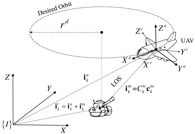
Figure 1: Loitering over a ground target.

II-A Dynamical Model of the GMT with Unknown Maneuver

The continuous-time version of the dynamical model of the GMT is given as

$$\begin{split}{\dot{x}^{t}}&={v^{tx}}\\ {\dot{y}^{t}}&={v^{ty}}\\ {\dot{v}^{tx}}&=u^{tx}+w^{tx}\\ {\dot{v}^{ty}}&=u^{ty}+w^{ty}\end{split}$$ (1)

where $[{x^{t}},{y^{t}},{v^{tx}},{v^{ty}}]^{T}$ denotes the position and the velocity of the GMT on the horizontal plane respectively, and $[u^{tx},u^{ty}]^{T}$ is the maneuver of the GMT. Moreover, $[w^{tx},w^{ty}]^{T}$ represents the random input noises, which are used to model the environmental disturbances.

Let $\tau$ be the sampling time interval. At time $k\tau$, we denote the state vector of the GMT as

$$\bm{x}_{k}^{t}=\begin{bmatrix}{x_{k}^{t}}&{y_{k}^{t}}&{z_{k}^{t}}&{v_{k}^{tx}}&{v_{k}^{ty}}\end{bmatrix}^{T}$$

where $z^{t}_{k}$ denotes the coordinate of the GMT in $Z$-axis. Since the ground is usually not an ideal plane and may be subject to random fluctuations, $z^{t}_{k}$ is time-varying as well. We model the fluctuations as a Gaussian random process with zero mean. Then, the discrete-time dynamical model of the GMT is compactly given as

$${\bm{x}}_{k+1}^{t}={{F}_{k}}\bm{x}_{k}^{t}+{{B}_{k}}\bm{u}^{t}({\gamma_{k}})+G_{k}{\bm{w}_{k}^{t}}$$ (2)

where

$${F_{k}}{\rm{=}}\begin{bmatrix}1&0&0&{\tau}&0\\ 0&1&0&0&{\tau}\\ 0&0&1&0&0\\ 0&0&0&1&0\\ 0&0&0&0&1\end{bmatrix},~{}{B_{k}}{\rm{=}}\begin{bmatrix}{\tau^{2}/2}&0\\ 0&{\tau^{2}/2}\\ 0&0\\ {\tau}&0\\ 0&{\tau}\end{bmatrix},~{}\text{and}~{}$$

$$~{}~{}~{}~{}~{}G_{k}{\rm{=}}\begin{bmatrix}{\tau^{2}/2}&0&0\\ 0&{\tau^{2}/2}&0\\ 0&0&{\tau}\\ {\tau}&0&0\\ 0&{\tau}&0\end{bmatrix}.$$

Moreover, $\{\bm{w}_{k}^{t}\}\subseteq{\mathbb{R}^{3}}$ are the white Gaussian input noises in X-axis and Y-axis, and the Gaussian fluctuations in Z-axis, i.e., ${\bm{w}_{k}^{t}}\sim{\mathcal{N}}(0,Q^{t})$.

Different from [1], the maneuver of the GMT is generally non-zero and is unknown to the UAV. In this work, the maneuver $\bm{u}^{t}({\gamma_{k}})\in{\mathbb{R}^{2}}$ is modeled as an unknown random vector [21]. Particularly, $\{\gamma_{k}\}$ is a three-state Markov chain, which corresponds to three modes of maneuver, e.g., keep straight, turn left, and turn right. Note that our results can be easily generalized to the case with any finite number of states if computational resource is sufficient, and this number directly imposes constraints on the motion of the GMT. In the simulation, we also validate the case with nine states.

Let $\mathcal{S}=\{1,2,3\}$ be the state space of the Markov chain $\{\gamma_{k}\}$, and denote its transition probability matrix by $P$, which actually can be estimated by the UAV with sensor measurements. For example, if we set

$$P=\begin{bmatrix}{0.9}&{0.05}&{0.05}\\ {0.05}&{0.9}&{0.05}\\ {0.05}&{0.05}&{0.9}\end{bmatrix},$$ (3)

then the probability that the GMT continues to be in the state of moving forward is 0.9 and the probability that the GMT turns left or right from the state of moving forward is 0.05. If $P$ is unknown, we simply set each element of $P$ as $1/3$. Without loss of generality, the GMT is initially set to be in the state of moving forward, i.e., $\gamma_{0}=1$.

II-B Dynamical Model of the UAV

We adopt a fixed-wing UAV to track the GMT, which is able to automatically keep its orientation stable. Compared to the flying altitude of the UAV, the fluctuations of the GMT in Z-axis is clearly small. Thus, we are only interested in the scenario that the motion of the UAV is restricted to a horizontal plane with a constant altitude. In [28], it provides a discrete-time dynamical model of a unicycle with a constant forward velocity. In this work, the forward velocity also needs to be controlled. Then, the discrete-time dynamical model of the UAV on the horizontal plane is described as

$$\begin{split}x_{k+1}^{a}&=x_{k}^{a}+\frac{1}{\tilde{u}_{k}^{a\psi}}\bigg{(}v_{k}^{a}(2\cos({\psi_{k}^{a}+\frac{\tilde{u}_{k}^{a\psi}\tau}{2}}){\rm{sin}}\frac{\tilde{u}_{k}^{a\psi}\tau}{2})\\ &~{}~{}~{}~{}+\tilde{u}_{k}^{av}\tau\sin(\psi_{k}^{a}+\tilde{u}_{k}^{a\psi}\tau)\\ &~{}~{}~{}~{}+\frac{\tilde{u}_{k}^{av}}{\tilde{u}_{k}^{a\psi}}(-2{\sin}(\psi_{k}^{a}+\frac{\tilde{u}_{k}^{a\psi}\tau}{2})\sin\frac{\tilde{u}_{k}^{a\psi}\tau}{2})\bigg{)},\\ y_{k+1}^{a}&=y_{k}^{a}+\frac{1}{\tilde{u}_{k}^{a\psi}}\bigg{(}2v_{k}^{a}(\sin(\psi_{k}^{a}+\frac{\tilde{u}_{k}^{a\psi}\tau}{2})\sin\frac{\tilde{u}_{k}^{a\psi}\tau}{2})\\ &~{}~{}~{}~{}-\tilde{u}_{k}^{av}\tau\cos(\psi_{k}^{a}+\tilde{u}_{k}^{a\psi}\tau)\\ &~{}~{}~{}~{}+\frac{\tilde{u}_{k}^{av}}{\tilde{u}_{k}^{a\psi}}(2{\rm{cos}}(\psi_{k}^{a}+\frac{\tilde{u}_{k}^{a\psi}\tau}{2}){\rm{sin}}\frac{\tilde{u}_{k}^{a\psi}\tau}{2})\bigg{)},\\ v_{{k}+1}^{a}&=v_{k}^{a}+{\tilde{u}}_{k}^{av}\tau,\\ \psi_{k+1}^{a}&=\psi_{k}^{a}+{\tilde{u}}_{k}^{a\psi}\tau,\end{split}$$ (4)

where $[x^{a}_{k},{y^{a}_{k}},\psi_{k}^{a},v^{a}_{k}]^{T}$ represents the coordinates, the heading direction, and the linear speed of the UAV on the plane, and ${\tilde{u}}_{k}^{av}={u}_{k}^{av}+{w}_{k}^{av}$ and ${\tilde{u}}_{k}^{a\psi}={u}_{k}^{a\psi}+{w}_{k}^{a\psi}$ are the perturbed commanded acceleration ($\mathrm{m}\mathrm{/}{\mathrm{s}^{2}}$) and turning rate ($\mathrm{r}\mathrm{a}\mathrm{d}\mathrm{/}\mathrm{s}$) respectively. Here $\bm{w}_{k}^{a}:=[w_{k}^{av},w_{k}^{a\psi}]^{T}\in\mathbb{R}^{2}$ represents the input disturbance, and is assumed to be bounded, i.e.

$$|w_{k}^{av}|\leq w^{v},~{}|w_{k}^{a\psi}|\leq w^{\psi}.$$ (5)

The motion of the UAV is also restricted [29, 30, 31], e.g. $\psi^{a}_{k}\in[-\pi,\pi)$, and

$$u_{k}^{a\psi}\in\mathcal{U}^{a\psi} :=\{u^{a\psi}\in\mathbb{R}:|u^{a\psi}|\leq u_{\max}^{a\psi}\}$$ (6)

where $u_{\max}^{a\psi}$ denotes the maximum angular speed of the UAV.

II-C Sensor Models in the UAV

To complete the loitering task, the UAV needs to be equipped with some necessary sensors. We first consider the camera sensor, and then the radar sensor, both of which are common in applications.

II-C1 Camera Sensor

A vision camera is amounted on a gimbal platform, which is to adjust the camera to keep the line of sight (LOS) towards the target. By using the controller in [32], the gimbal platform can maintain the GMT in the field of vision (FOV) of the camera to avoid the target loss. Thus, we directly assume that the GMT is always in the FOV of the vision camera, and is treated as a pure mass point.

The camera projects a target point ${\bm{p}}:=[x,y,z]^{T}$ in 3D coordinates into a pixel point $[b,c]^{T}$ on the 2D camera image plane, see Fig. 2 for illustrations.

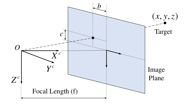
Figure 2: Camera perspective projection model.

The measurement model [1] of the camera is thus expressed as

$${\bm{h}}^{c}({\bm{p}}):=\begin{bmatrix}b\\ c\end{bmatrix}=\frac{f}{x}\begin{bmatrix}y\\ z\end{bmatrix}$$ (7)

where $f$ is the camera focal length, and the image processing software can automatically produce the coordinate $[b,c]^{T}$ once the target is locked. To improve the image quality, we need to keep the object distance invariant.

The coordinate $x=0$ corresponds to that the target point $[x,y,z]^{T}$ is exactly on the camera image plane, which is impossible here. Moreover, the Jacobian matrix of ${\bm{h}}^{c}({\bm{p}})$ is easily computed as

$$J^{c}({\bm{p}})=\frac{f}{x^{2}}\begin{bmatrix}-y&x&0\\ -z&0&x\end{bmatrix}.$$ (8)

II-C2 Radar Sensor

A radar sensor is able to provide the range and azimuth measurements between the radar and the target. Its measurement model can be expressed as

$${\bm{h}}^{r}({\bm{p}}):=\begin{bmatrix}d\\ \varphi\end{bmatrix}=\begin{bmatrix}{({x^{2}}+{y^{2}}+{z^{2}})^{1/2}}\\ {\arctan({y}/{x})}\end{bmatrix},$$ (9)

where $d$ and the angle $\varphi$ are range and azimuth measurements of the radar. Similarly, the Jacobian matrix of ${\bm{h}}^{r}({\bm{p}})$ is easily computed as

$$J^{r}({\bm{p}})=\begin{bmatrix}x/d&y/d&z/d\\ -y/(x^{2}+y^{2})&x/(x^{2}+y^{2})&0\end{bmatrix}.$$ (10)

II-D The Objective of This Work

The main objective of this paper is to design a flight controller for the UAV to loiter over the GMT by using a camera or radar sensor.

To achieve it, we design a tracking system as shown in Fig. 3, which is mainly composed of a discrete-time guidance law, a discrete-time controller, and a motion estimator. It is worth mentioning that the state $\bm{x}_{k}^{a}$ of the UAV can be directly obtained by the navigation system, e.g., the position and orientation system (POS). The POS always consists of an inertial measurement unit (IMU) and a Global Navigation Satellite System (GNSS). The control of the gimbal platform has also been separately studied in [32]. Thus, both the gimbal control and navigation are not the focus of this work.

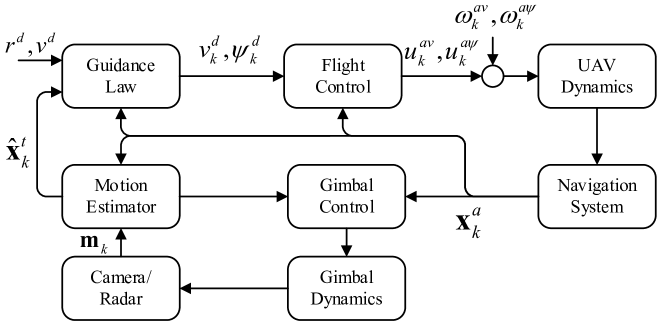
Figure 3: Structure of the overall system.

Overall, the flight control problem of this work includes at least the following challenging issues: (a) the discrete-time guidance law for the UAV, which extends the continuous-time guidance law in [1] to the discrete-time case; (b) the control of the UAV to track the guidance trajectory. Since disturbances are unavoidable in the whole system, the controller should be of sufficient robustness to uncertainties; (c) the motion state estimation of the GMT in the presence of the unknown maneuver, which requires to simultaneously estimate the maneuver and the motion state.

III Discrete-time Guidance Law

The discrete-time guidance law guides the UAV to loiter over the GMT with a desired radius at a relative constant speed. In [33], a continuous-time Lyapunov guidance vector field is proposed for a static target, which is extended to the case of a moving target with a constant velocity in [6] and [12]. Note that they all need the states of both the UAV and the GMT. Here, we design a discrete-time Lyapunov guidance vector field to direct the UAV to loiter over the GMT with a desired radius $r^{d}$ at a relative constant speed $v^{d}$.

If the states of both the UAV and the GMT are available, let $x_{k}=x_{k}^{a}-x_{k}^{t}$ and $y_{k}=y_{k}^{a}-y_{k}^{t}$ represent the relative positions between the GMT and the UAV in X-axis and Y-axis, respectively. For a sampling period $\tau>0$, then

$$v_{k}^{x}=\frac{x_{k+1}-x_{k}}{\tau}~{}\text{and}~{}v_{k}^{y}=\frac{y_{k+1}-y_{k}}{\tau}$$

are the relative velocities between the GMT and the UAV in X-axis and Y-axis.

Figure 4: Illustration of the discrete-time Lyapunov guidance vector method.

Given two positive constants $r^{d}$ and $v^{d}$, the discrete-time guidance vector is given by the following dynamical equation

$$\begin{bmatrix}v_{k}^{x}\\ v_{k}^{y}\end{bmatrix}=\frac{{-v^{d}}}{r_{k}\big{(}(r_{k})^{2}+(r^{d})^{2}\big{)}}\begin{bmatrix}{{x_{k}}\big{(}(r_{k})^{2}-(r^{d})^{2}\big{)}+{y_{k}}(2r^{d}r_{k})}\\ {{y_{k}}\big{(}(r_{k})^{2}-(r^{d})^{2}\big{)}-{x_{k}}(2r^{d}r_{k})}\end{bmatrix}$$ (11)

where $r_{k}=({(x_{k})^{2}}+{(y_{k})^{2}})^{1/2}$ denotes the projected relative distance between the GMT and the UAV onto the X-Y plane.

Moreover, if the sampling interval $\tau$ is sufficiently small or the sampling frequency $1/\tau$ is fast enough, and the desired angular speed $v^{d}/r^{d}$ is not too large, i.e.,

$$\frac{v^{d}}{r^{d}}<u_{\max}^{a\psi}~{}\text{and}~{}\frac{1}{\tau}>\frac{\sqrt{3}u_{\max}^{a\psi}}{2}$$ (12)

where $u_{\max}^{a\psi}$, defined in (6), is the maximum angular speed of the UAV, then we show below that $r^{d}$ is the desired radius of the loitering orbit, and $v^{d}$ is the desired loitering speed.

To this end, we first provide an intuitive explanation on the discrete-time guidance vector in (11). Let $\alpha_{k}$ denote the angle between the relative position vector $[x_{k},y_{k}]^{T}$ and relative velocity vector $[v^{x}_{k},v^{y}_{k}]^{T}$. Then, its cosine can be computed as

$$\cos\alpha_{k} = \frac{x_{k}v^{x}_{k}+y_{k}v^{y}_{k}}{\sqrt{(x_{k})^{2}+(y_{k})^{2}}{\sqrt{(v^{x}_{k})^{2}+(v^{y}_{k})^{2}}}}$$ (13)

$$= -\frac{(r_{k})^{2}-(r^{d})^{2}}{(r_{k})^{2}+(r^{d})^{2}}$$

where the first equality follows from the definition of the angle between two vectors, and the second equality is derived by using the design of $[v^{x}_{k},v^{y}_{k}]^{T}$ in (11).

If $0<r_{k}<r^{d}$, it follows from (13) that $\cos\alpha_{k}>0$ and ${\pi}/{2}>\alpha_{k}>0$. Then, the projected relative distance $r_{k}$ increases towards the desired radius. On the other side, if $r_{k}>r^{d}$, then $\cos\alpha_{k}<0$ and $\alpha_{k}>{\pi}/{2}$. This implies that $r_{k}$ decreases towards the desired radius. If $r_{k}=r^{d}$, then $\cos\alpha_{k}=0$, and $\alpha_{k}={\pi}/{2}$, the relative velocity $[v^{x}_{k},v^{y}_{k}]^{T}$ is exactly orthogonal to the relative position vector $[x_{k},y_{k}]^{T}$. Then, the UAV loiters over the GMT with the desired radius $r^{d}$ at the relative speed $v^{d}$. See Fig. 4 for a graphical illustration.

Now, we are in the position to provide a rigorous proof of the above observation.

Theorem 1

If the relative position $[x_{k},y_{k}]^{T}$ and velocity $[v_{k}^{x},v_{k}^{y}]^{T}$ on the X-Y plane are designed via the discrete-time guidance law (11) where $r^{d}$ and $v^{d}$ satisfy (12), the UAV eventually loiters over the GMT with a desired radius $r^{d}$ at an angular speed $v^{d}/r^{d}$.

Proof:

Let the coordinates $x_{k}$ and $y_{k}$ be converted to the polar coordinates $r_{k}$ and $\theta_{k}$ by using the trigonometric functions, i.e.,

$$x_{k} =r_{k}\cos\theta_{k},$$

$$y_{k} =r_{k}\sin\theta_{k}.$$

Then, the discrete-time vector field of (11) in the polar coordinates is given as

$$\begin{bmatrix}{\Delta r_{k}}\\ {{r_{k}}\Delta{\theta_{k}}}\end{bmatrix}=-v^{d}{\tau}\begin{bmatrix}\displaystyle{\frac{(r_{k})^{2}-(r^{d})^{2}}{(r_{k})^{2}+(r^{d})^{2}}}\\ \displaystyle{\frac{-2r^{d}r_{k}}{(r_{k})^{2}+(r^{d})^{2}}}\end{bmatrix}$$ (14)

where $\Delta r_{k}=r_{k+1}-r_{k}$ and $\Delta{\theta_{k}}=\theta_{k+1}-\theta_{k}$.

Consider the following Lyapunov function candidate

$${V(r_{k})}=\frac{1}{2}\left((r_{k})^{2}-(r^{d})^{2}\right)^{2}.$$

Then, taking the difference of $V(r_{k})$ along (11) leads to that

$$\Delta{V(r_{k})} ={V(r_{k+1})}-{V(r_{k})}$$

$$=\frac{1}{2}\left((r_{k+1})^{2}+(r_{k})^{2}-2(r^{d})^{2}\right)(r_{k+1}+r_{k})(\Delta r_{k})$$

$$=\frac{1}{2}(r_{k+1}+r_{k})(\Delta r_{k})^{2}\big{(}2\frac{(r_{k})^{2}+(r^{d})^{2}}{-{v^{d}}\tau}+$$

$$~{}~{}~{}~{}\Delta r_{k}+2r_{k}\big{)}$$

$$=-\frac{1}{2}(r_{k+1}+r_{k})(\Delta r_{k})^{2}\big{(}2\frac{(r_{k})^{2}+(r^{d})^{2}}{{v^{d}}\tau}-2r_{k}+$$

$$~{}~{}~{}~{}v^{d}\tau\frac{(r_{k})^{2}-(r^{d})^{2}}{(r_{k})^{2}+(r^{d})^{2}}\big{)}.$$ (15)

Since $-1\leq\displaystyle\frac{(r_{k})^{2}-(r^{d})^{2}}{(r_{k})^{2}+(r^{d})^{2}}<1$, then $v^{d}\tau\displaystyle\frac{(r_{k})^{2}-(r^{d})^{2}}{(r_{k})^{2}+(r^{d})^{2}}\geq-v^{d}\tau,$ which together with (15) implies that

$$\Delta{V(r_{k})} \leq-\frac{1}{2}(r_{k+1}+r_{k})(\Delta r_{k}^{2})\frac{1}{v^{d}\tau}\big{(}2(r_{k})^{2}-2{v^{d}}\tau r_{k}$$

$$~{}~{}~{}~{}+2(r^{d})^{2}-{({v^{d}}\tau)^{2}}\big{)}.$$

Thus, the sign of $\Delta{V(r_{k})}$ is determined by the following quadratic term

$$2(r_{k})^{2}-2{v^{d}}\tau r_{k}+2(r^{d})^{2}-{({v^{d}}\tau)^{2}}.$$ (16)

By (12), one can easily verify that $(-2{v^{d}}\tau)^{2}-4\times 2\times\left(2(r^{d})^{2}-({v^{d}}\tau)^{2}\right)<0$, which implies that (16) is always positive for any $r_{k}$.

By combining the above, it finally holds that

$$\Delta V(r_{k})\leq 0.$$

Moreover, $V(r_{k})$ has the following three properties

• (nonnegative) $V(r^{d})=0$ and $V(r_{k})>0$, $\forall r_{k}\not=r^{d}$,

• (strictly decreasing) $\Delta V(r_{k})<0$, $\forall r_{k}\not=r^{d}$,

• (radially unbounded) if $r_{k}\rightarrow\infty$, then $V(r_{k})\rightarrow\infty$.

By the discrete-time version of Theorem 4.2 in [34], then $r_{k}=r^{d}$ is an equilibrium point, which is also globally asymptotically stable. That is, $\lim_{k\rightarrow\infty}r_{k}=r^{d}$. This implies that the relative distance $r_{k}$ on the X-Y plane between the UAV and the GMT eventually converges to the desired radius $r^{d}$.

In view of (14), it follows that $(\Delta r_{k})^{2}+(r_{k}\Delta\theta_{k})^{2}=(v^{d}\tau)^{2}$. When the UAV is flying on the circular orbit, i.e. $\Delta r_{k}=0$, it only has the tangential speed $(r_{k}\Delta\theta_{k})/\tau$, which is equal to $v^{d}$.  

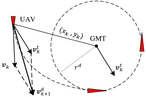
Figure 5: The discrete-time guidance vector field.

If the state of the GMT is known, the desired speed and heading angle of the UAV in the inertial frame is given as

$$\begin{split}v^{d}_{k+1}&=\sqrt{(v_{k}^{tx}+v_{k}^{x})^{2}+(v_{k}^{ty}+v_{k}^{y})^{2}},\\ {\psi^{d}_{k+1}}&=\arctan\frac{v_{k}^{ty}+v_{k}^{y}}{v_{k}^{tx}+v_{k}^{x}},\end{split}$$ (17)

where $\bm{v}_{k}^{t}=[v_{k}^{tx},v_{k}^{ty}]^{T}$ is the velocity of the GMT, and the relative velocity $\bm{v}_{k}=[v_{k}^{x},v_{k}^{y}]^{T}$ on the X-Y plane is designed in (11). See Fig. 5 for illustrations.

IV Discrete-time Integral SMC with Perfect State of the GMT

In this section, we design the controller for the UAV to asymptotically track the guidance commands $\{v^{d}_{k}\}$ and $\{\psi^{d}_{k}\}$ in (17). To handle the disturbance $\bm{w}_{k}^{a}$, we design a discrete-time integral sliding model controller (ISMC), which is different from the continuous-time proportional-derivative (PD) controller in [1, 12]. Usually, the ISMC has strong robustness to system uncertainties and external disturbances.

Define the tracking errors of the desired speed and heading angle by

$${\bm{e}_{k}}:=\begin{bmatrix}{e_{k}^{v}}&{e_{k}^{\psi}}\end{bmatrix}^{T}=\begin{bmatrix}{v^{a}_{k}-v_{k}^{d}}\\ {\psi^{a}_{k}-\psi_{k}^{d}}\end{bmatrix}$$

where $[v_{k}^{d},\psi_{k}^{d}]^{T}$ is given in (17). Together with the UAV dynamics in (4), the dynamical equation of the tracking errors can be written as follows

$${\bm{e}_{k+1}}=\begin{bmatrix}{e_{k+1}^{v}}\\ {e_{k+1}^{\psi}}\end{bmatrix}=\begin{bmatrix}{e^{v}_{k}+u_{k}^{av}\tau+w_{k}^{av}\tau-\Delta v_{k}^{d}}\\ {e^{\psi}_{k}+u_{k}^{a\psi}\tau+w_{k}^{a\psi}\tau-\Delta\psi_{k}^{d}}\end{bmatrix}$$ (18)

where $\Delta v_{k}^{d}=v_{k+1}^{d}-v_{k}^{d}$ and $\Delta\psi_{k}^{d}=\psi_{k+1}^{d}-\psi_{k}^{d}$. Then, the flight controller of the UAV is designed by using the ISMC, which is explicitly given below

$$\begin{bmatrix}{u_{k}^{av}}\\ {u_{k}^{a\psi}}\end{bmatrix}=-W\text{sgn}({\bm{s}_{k}})-{M}\bm{s}_{k}-{C}\bm{e}_{k}+\frac{1}{\tau}\begin{bmatrix}{\Delta v_{k}^{d}}\\ {\Delta\psi_{k}^{d}}\end{bmatrix}$$ (19)

where the diagonal matrices ${W}=\text{diag}({{w^{v}}},{{w^{\psi}}})$, ${M}=\text{diag}({{m^{v}}},{{m^{\psi}}})$, and $C=\text{diag}({c^{v}},{c^{\psi}})$ are to be designed, and the sign function ${\rm sgn}({s})$ is defined as

$${\rm sgn}(s)=\left\{{\begin{array}[]{*{20}{c}}{~{}~{}1,}&{s>0,}\\ {~{}~{}0,}&{s=0,}\\ {-1,}&{s<0.}\end{array}}\right.$$

Moreover, the discrete-time integral sliding mode surface is designed as

$${\bm{s}_{k}}=[{s_{k}^{v}}~{}~{}{s_{k}^{\psi}}]^{T}=\bm{e}_{k}+\tau{C}\sum\limits_{i=0}^{k-1}{\bm{e}_{i}}.$$ (20)

Before proving the effectiveness of the ISMC in (19), we introduce some notations in this section. For a vector ${\bm{x}}$, then $|{\bm{x}}|$ takes the absolute values over every element of ${\bm{x}}$, $\text{sgn}({\bm{x}})$ applies the sign function to each element of ${\bm{x}}$, and $\text{diag}({\bm{x}})$ is a diagonal matrix whose diagonal element exactly corresponds to each element of ${\bm{x}}$. For two vectors ${\bm{x}}$ and ${\bm{y}}$, the relation ${\bm{x}}\succ{\bm{y}}$ (${\bm{x}}\prec{\bm{y}}$) means that each element of ${\bm{x}}$ is strictly greater (less) than the element of the same position in ${\bm{y}}$.

Theorem 2

Consider the discrete-time dynamical model of the UAV in (4). Under the ISMC in (19) and select the design parameters as follows: $0<c^{v},c^{\psi}<1/\tau$, $0<m^{v},m^{\psi}<1/\tau$. Then, the UAV asymptotically tracks the guidance commands $[v_{k}^{d},\psi_{k}^{d}]^{T}$ in (17) with the tracking error $\bm{e}_{k}$ satisfying that

$$\limsup_{k\rightarrow\infty}|\bm{e}_{k}|\prec 4C^{-1}(2I-\tau M)^{-1}\begin{bmatrix}{w^{v}}\\ {w^{\psi}}\end{bmatrix},$$

where $w^{v}$ and $w^{\psi}$ are given in (5). Moreover, if $2C=2M=\frac{1}{\tau}I$, then

$$\limsup_{k\rightarrow\infty}|\bm{e}_{k}|\prec\frac{16}{3}\tau\begin{bmatrix}{w^{v}}\\ {w^{\psi}}\end{bmatrix}.$$

Proof:

Clearly, the discrete-time exponential reaching law is expressed as

$$\Delta{\bm{s}_{k}}={\bm{s}_{k+1}}-{\bm{s}_{k}}=-\tau W\text{sgn}({\bm{s}_{k}})-\tau M{\bm{s}_{k}}.$$ (21)

Together with the ISMC in (19), we can easily obtain that

$${\bm{s}_{k+1}}=(I-\tau M){\bm{s}_{k}}-\tau W\text{sgn}({\bm{s}_{k}})+\tau\bm{w}_{k}^{a}.$$ (22)

Define a Lyapunov function candidate as

$$V^{s}(\bm{s}_{k})=\frac{1}{\tau}\bm{s}_{k}^{T}\bm{s}_{k}.$$

Taking the difference of $V^{s}(\bm{s}_{k})$ along (22), we can obtain that

$$\Delta V^{s}(\bm{s}_{k})=V^{s}(\bm{s}_{k+1})-V^{s}(\bm{s}_{k})$$ (23)

$$=(\bm{s}_{k+1}+\bm{s}_{k})^{T}\big{(}-M{\bm{s}_{k}}-W\text{sgn}({\bm{s}_{k}})+\bm{w}_{k}^{a}\big{)}$$

$$\leq-(\bm{s}_{k+1}+\bm{s}_{k})^{T}(M{\bm{s}_{k}})-(\bm{s}_{k+1}+\bm{s}_{k})^{T}W\text{sgn}({\bm{s}_{k}})$$

$$~{}~{}~{}~{}+|\bm{s}_{k+1}+\bm{s}_{k}|^{T}(\begin{bmatrix}w^{v},w^{\psi}\end{bmatrix}^{T})$$

$$=-(\bm{s}_{k+1}+\bm{s}_{k})^{T}(M{\bm{s}_{k}})$$

$$~{}~{}~{}~{}-(\bm{s}_{k+1}+\bm{s}_{k})^{T}W(\text{sgn}({\bm{s}_{k}})-\text{sgn}({\bm{s}_{k}}+{\bm{s}_{k+1}})).$$

If $\text{diag}(\bm{s}_{k+1}+\bm{s}_{k})\text{sgn}({\bm{s}_{k}})\succ 0$, it holds that $(\bm{s}_{k+1}+\bm{s}_{k})^{T}\text{sgn}({\bm{s}_{k}})>0$. Together with (22), we have

$$\text{diag}(\bm{s}_{k+1}+\bm{s}_{k})\text{sgn}({\bm{s}_{k}})$$

$$=\text{diag}\big{(}(2I-\tau M)\bm{s}_{k}-\tau W\text{sgn}(\bm{s}_{k})+\tau\bm{w}_{k}^{a}\big{)}\text{sgn}({\bm{s}_{k}})$$

$$\geq\text{diag}\big{(}(2I-\tau M)\bm{s}_{k}\big{)}\text{sgn}(\bm{s}_{k})-2\tau(\text{diag}(w^{v},w^{\psi}))|\text{sgn}(\bm{s}_{k})|$$

$$=(2I-\tau M)|\bm{s}_{k}|-2\tau\begin{bmatrix}w^{v},w^{\psi}\end{bmatrix}^{T}$$

Thus, if $|{\bm{s}}_{k}|\succ(2I-\tau M)^{-1}(2\tau\begin{bmatrix}w^{v},w^{\psi}\end{bmatrix}^{T})$, the reaching condition holds, i.e.,

$$\text{diag}(\bm{s}_{k+1}+\bm{s}_{k})\text{sgn}(\bm{s}_{k})\succ 0,$$ (24)

which implies that $\text{sgn}(\bm{s}_{k})=\text{sgn}(\bm{s}_{k+1}+\bm{s}_{k})$. Together with (23), it follows that $\Delta V^{s}(\bm{s}_{k})<0$. That is, the boundary layer is attractive. By [35], there exists a finite time $k_{0}$ such that

$$|{\bm{s}}_{k}|\prec(2I-\tau M)^{-1}(2\tau\begin{bmatrix}w^{v},w^{\psi}\end{bmatrix}^{T}),\forall k\geq{k_{0}}.$$ (25)

Next, we show that the tracking error ${\bm{e}}_{k}$ will also be attracted to a bounded region. To elaborate it, let $\Delta{\bm{e}}_{k}:={\bm{e}}_{k+1}-{\bm{e}}_{k}$. It follows from (20) that

$$\bm{e}_{k}=\bm{s}_{k}-\tau{C}\sum\limits_{i=0}^{k-1}{\bm{e}_{i}}$$

and $\Delta\bm{e}_{k}=\bm{s}_{k+1}-\bm{s}_{k}-\tau C\bm{e}_{k}$.

For any $k\geq k_{0}$, the above implies that

$$\bm{e}_{k+1} =(I-\tau C)\bm{e}_{k}+\Delta\bm{s}_{k}$$

$$=(I-\tau C)^{k+1}\bm{e}_{0}+\sum_{i=0}^{k}(I-\tau C)^{k-i}\Delta\bm{s}_{i}$$

$$=(I-\tau C)^{k+1}\bm{e}_{0}+\sum_{i=0}^{k_{0}-1}(I-\tau C)^{k-i}\Delta\bm{s}_{i}$$

$$~{}~{}~{}~{}~{}+\sum_{i=k_{0}}^{k}(I-\tau C)^{k-i}\Delta\bm{s}_{i}.$$ (26)

In light of (21) and (25), it is clear that

$$|\Delta{\bm{s}}_{k}|\prec 4\tau(2I-\tau M)^{-1}\begin{bmatrix}{w^{v}},{w^{\psi}}\end{bmatrix}^{T},\forall k\geq k_{0}.$$

Thus, $\Delta\bm{s}_{i}$ is uniformly bounded. Since the spectral radius of $I-\tau C$ is strictly less than one, it implies that $\lim_{k\rightarrow\infty}(I-\tau C)^{k+1}\bm{e}_{0}=0$, $\lim_{k\rightarrow\infty}\sum_{i=0}^{k_{0}-1}(I-\tau C)^{k-i}\Delta\bm{s}_{i}=0$ and

$$\left|\sum_{i=k_{0}}^{k}(I-\tau C)^{k-i}\Delta\bm{s}_{i}\right|$$

$$\prec 4\tau\sum_{i=k_{0}}^{k}(I-\tau C)^{k-i}(2I-\tau M)^{-1}\begin{bmatrix}{w^{v}},{w^{\psi}}\end{bmatrix}^{T}$$

$$\prec 4\tau\sum_{i=0}^{\infty}(I-\tau C)^{i}(2I-\tau M)^{-1}\begin{bmatrix}{w^{v}},{w^{\psi}}\end{bmatrix}^{T}$$

$$\prec 4C^{-1}(2I-\tau M)^{-1}\begin{bmatrix}{w^{v}},{w^{\psi}}\end{bmatrix}^{T}.$$

Together with (IV), it follows that

$$\limsup_{k\rightarrow\infty}|\bm{e}_{k+1}|\prec 4C^{-1}(2I-\tau M)^{-1}\begin{bmatrix}{w^{v}},{w^{\psi}}\end{bmatrix}^{T}.$$

The rest of the proof is trivial.  

By Theorem 2, the tracking error is proportional to the sampling period $\tau$ and the size of disturbances to the UAV, which clearly is consistent with our intuition.

V Motion Estimation of the GMT with Unknown Maneuver

If the state of the GMT is perfectly known, we have designed the discrete-time guidance law and the ISMC for the UAV in the previous sections. Since the GMT can be an intruder or enemy, it is impossible for the UAV to access its exact maneuver and thus the state cannot be accurately obtained. From the tracking system in Fig. 3, it is clear that the motion estimation is vital for the guidance law, the flight control and the gimbal control for stabilizing the camera sensor. If the maneuver is known, the state estimation problem of the GMT is well studied by using the standard nonlinear filters, e.g., EKF, Unscented Kalman filter (UKF) or PF [36]. To address this case with unknown maneuver, we consider using a Markov chain to model the maneuver process in Section II-A, and adopting our recently proposed Rao-Blackwellised particle filter (RBPF) [22] to simultaneously estimate both the maneuver modes $\gamma_{k}$ and the state of the GMT. Compared to the standard PF, the number of sampling particles for the RBPF is much smaller.

V-A State Estimation of the GMT

In virtue of (2), the discrete-time dynamical model of the GMT and the measurement equation are collectively given as

$$\begin{split}{\bm{x}}_{k+1}^{t}&={{F}_{k}}\bm{x}_{k}^{t}+{{B}_{k}}\bm{u}^{t}({\gamma_{k}})+G_{k}{\bm{w}_{k}}\\ \bm{m}_{k}&={\bm{h}}(\bm{x}_{k}^{t})+\bm{v}_{k}\end{split}$$ (27)

where $\bm{m}_{k}\in\mathbb{R}^{2}$ is the measurement of the UAV by using a camera or a radar sensor and $\{\bm{v}_{k}\}$ is the measurement Gaussian white noise, i.e., ${\bm{v}_{k}}\sim{\mathcal{N}}(0,R)$.

Define $\mathit{\Gamma}_{k}=\{\gamma_{0},...,\gamma_{k}\}$, $\mathcal{M}_{k}=\{\bm{m}_{0},...,\bm{m}_{k}\}$. Recall that the minimum variance estimate of $\bm{x}_{k}^{t}$ is given as

$$\begin{split}\bm{\widehat{x}}_{k|k}^{t}&=\int{\bm{x}_{k}^{t}}p(\bm{x}_{k}^{t}|\mathcal{M}_{k})\mathrm{d}\bm{x}_{k}^{t}\\ &=\iint{\bm{x}_{k}^{t}}p(\bm{x}_{k}^{t},\mathit{\Gamma}_{k-1}|\mathcal{M}_{k})\mathrm{d}\bm{x}_{k}^{t}\mathrm{d}\mathit{\Gamma}_{k-1}.\end{split}$$ (28)

Notice that $p(\bm{x}_{k}^{t},\mathit{\Gamma}_{k-1}|\mathcal{M}_{k})$ is not Gaussian and is impossible to be analytically obtained. Thus, the integral is not computable and we have to resort to a numerical approach.

To exposit it, it follows from the law of total probability that

$$p(\bm{x}_{k}^{t},\mathit{\Gamma}_{k-1}|\mathcal{M}_{k})=p(\bm{x}_{k}^{t}|\mathit{\Gamma}_{k-1},\mathcal{M}_{k})p(\mathit{\Gamma}_{k-1}|\mathcal{M}_{k})$$

where $p(\bm{x}_{k}^{t}|\mathit{\Gamma}_{k-1},\mathcal{M}_{k})$ is approximately computed by the extended Kalman filter (EKF) in a recursive form [37].

However, $p(\mathit{\Gamma}_{k-1}|\mathcal{M}_{k})$ is inherently difficult to obtain. As $\mathit{\Gamma}_{k-1}$ is a ternary-valued sequence, we draw $n$ particles $\{\mathit{\Gamma}_{k-1}^{i}\}_{i=1}^{n}$ from an importance distribution $q(\mathit{\Gamma}_{k-1}|\mathcal{M}_{k})$ to approximately compute $p(\mathit{\Gamma}_{k-1}|\mathcal{M}_{k})$, i.e.,

$$p(\mathit{\Gamma}_{k-1}|\mathcal{M}_{k})\approx\sum\limits_{i=1}^{n}{\omega_{k-1}^{i}}\delta(\mathit{\Gamma}_{k-1}-\mathit{\Gamma}_{k-1}^{i})$$ (29)

where $\delta(\cdot)$ is the standard Dirac delta function and the normalized particle weight $\omega_{k-1}^{i}$ is associated with $\mathit{\Gamma}_{k-1}^{i}$, which is given as

$$\omega_{k-1}^{i}\propto\frac{{p(\mathit{\Gamma}_{k-1}^{i}|\mathcal{M}_{k})}}{{q(\mathit{\Gamma}_{k-1}^{i}|\mathcal{M}_{k})}}.$$ (30)

Combining (28) with (29), we obtain that

$$\widehat{\bm{x}}_{k|k}^{t}\approx\sum\limits_{i=1}^{n}{\omega_{k-1}^{i}}\mathbb{E}[\bm{x}_{k}^{t}|\mathit{\Gamma}_{k-1}^{i},\mathcal{M}_{k}].$$

Similarly, the estimation error covariance matrix is given as

$${\Sigma}_{k|k}^{t}\approx\sum\limits_{i=1}^{n}{\omega_{k-1}^{i}}\mathbb{E}[(\bm{x}_{k}^{t}-\widehat{\bm{x}}_{k|k}^{t}){(\bm{x}_{k}^{t}-\widehat{\bm{x}}_{k|k}^{t})^{T}}|\mathit{\Gamma}_{k-1}^{i},\mathcal{M}_{k}].$$

Let $\widehat{\bm{x}}_{k|k}^{i}:=\mathbb{E}[\bm{x}_{k}^{t}|\mathit{\Gamma}_{k-1}^{i},\mathcal{M}_{k}]$ and ${\Sigma}_{k|k}^{i}:=\mathbb{E}[(\bm{x}_{k}^{t}-\widehat{\bm{x}}_{k|k}^{i}){(\bm{x}_{k}^{t}-\widehat{\bm{x}}_{k|k}^{i})^{T}}|\mathit{\Gamma}_{k-1}^{i},\mathcal{M}_{k}]$. It should be noted that $\widehat{\bm{x}}_{k|k}^{i}$ and $\Sigma_{k|k}^{i}$ can be approximately computed by the EKF, i.e.,

$$\widehat{\bm{x}}_{k|k}^{i}\approx\widehat{\bm{x}}_{k|k-1}^{i}+K_{k}^{i}(\bm{m}_{k}-{\bm{h}}(\widehat{\bm{x}}_{k|k-1}^{i}))$$

$${\Sigma}_{k|k}^{i}\approx{\Sigma}_{k|k-1}^{i}-K_{k}^{i}H_{k}^{i}{\Sigma}_{k|k-1}^{i}$$ (31)

where $K_{k}^{i}={\Sigma}_{k|k-1}^{i}(H_{k}^{i})^{T}(H_{k}^{i}{\Sigma}_{k|k-1}^{i}(H_{k}^{i})^{T}+R)^{-1}$ and the Jacobian matrix evaluated at $\widehat{\bm{x}}_{k|k-1}^{i}$ is

$$H_{k}^{i}=\frac{\partial}{\partial\bm{x}_{k}^{t}}{\bm{h}}(\bm{x}_{k}^{t})|_{\bm{x}_{k}^{t}=\widehat{\bm{x}}_{k|k-1}^{i}}.$$ (32)

The remaining problem is how to recursively generate particles $\{\mathit{\Gamma}_{k-1}^{i}\}$ and compute their associated weights $\{\omega_{k-1}^{i}\}$.

V-B Importance Distribution

If an importance distribution is chosen to factorize such that

$$q(\mathit{\Gamma}_{k-1}|\mathcal{M}_{k})=q({\gamma_{k-1}}|\mathit{\Gamma}_{k-2},\mathcal{M}_{k})q(\mathit{\Gamma}_{k-2}|\mathcal{M}_{k-1}).$$ (33)

Then, the particles $\mathit{\Gamma}_{k-1}^{i}\sim q(\mathit{\Gamma}_{k-1}|\mathcal{M}_{k})$ can be obtained by augmenting each existing particle $\mathit{\Gamma}_{k-2}^{i}\sim q(\mathit{\Gamma}_{k-2}|\mathcal{M}_{k-1})$ with the new state $\gamma_{k-1}^{i}\sim q({\gamma_{k-1}}|\mathit{\Gamma}_{k-1},\mathcal{M}_{k})$, recursively [22]. To elaborate it, we express $p(\mathit{\Gamma}_{k-1}|\mathcal{M}_{k})$ in the following form

$$p(\mathit{\Gamma}_{k-1}|\mathcal{M}_{k})$$

$$\propto p({\bm{m}_{k}}|\mathit{\Gamma}_{k-1},\mathcal{M}_{k-1})p({\gamma_{k-1}}|\mathit{\Gamma}_{k-2},\mathcal{M}_{k-1})p(\mathit{\Gamma}_{k-2}|\mathcal{M}_{k-1}).$$

Jointly with (30), it implies that

$$\begin{split}&\omega_{k-1}^{i}\\ &\propto\frac{{p({\bm{m}_{k}}|\mathit{\Gamma}_{k-1}^{i},\mathcal{M}_{k-1})p(\gamma_{k-1}^{i}|\mathit{\Gamma}_{k-2}^{i},\mathcal{M}_{k-1})p(\mathit{\Gamma}_{k-2}^{i}|\mathcal{M}_{k-1})}}{{q({\gamma_{k}}|\Gamma_{k-2}^{i},\mathcal{M}_{k})q(\mathit{\Gamma}_{k-2}^{i}|\mathcal{M}_{k-1})}}\\ &=\omega_{k-2}^{i}\frac{{p({\bm{m}_{k}}|\mathit{\Gamma}_{k-1}^{i},\mathcal{M}_{k-1})p(\gamma_{k-1}^{i}|\mathit{\Gamma}_{k-2}^{i},\mathcal{M}_{k-1})}}{{q(\gamma_{k-1}^{i}|\mathit{\Gamma}_{k-2}^{i},\mathcal{M}_{k})}}\end{split}$$

where $p({\bm{m}_{k}}|\mathit{\Gamma}_{k-1}^{i},\mathcal{M}_{k-1})$ is an approximately conditional Gaussian density, e.g.,

$$p({\bm{m}_{k}}|\mathit{\Gamma}_{k-1}^{i},\mathcal{M}_{k-1})\approx{\mathcal{N}}({\bm{h}}(\widehat{\bm{x}}_{k|k-1}^{i}),H_{k}^{i}\Sigma_{k|k-1}^{i}(H_{k}^{i})^{T}+R).$$ (34)

The degeneracy problem is essential to the success of particle sampling. To alleviate it, there are two approaches of selecting the important distribution $q(\gamma_{k-1}|\mathit{\Gamma}_{k-2}^{i},\mathcal{M}_{k})$[36]. One is $p(\gamma_{k-1}|\mathit{\Gamma}_{k-2}^{i},\mathcal{M}_{k})$, which minimizes a suitable measure of the degeneracy of the algorithm. The other is $p(\gamma_{k-1}|\gamma_{k-2}^{i})$, which makes it easy to draw particles and compute the importance weights.

We choose the later one as the importance distribution, e.g., $q(\gamma_{k-1}|{\mathit{\Gamma}^{i}_{k-2}},{\mathcal{M}_{k}})=p(\gamma_{k-1}|\gamma_{k-2}^{i})$ to simplify the process of drawing samples. Specifically, the new particle is generated via the following distribution

$$\gamma_{k-1}^{i}\sim p(\gamma_{k-1}|\gamma_{k-2}^{i}),$$ (35)

which is explicitly given in (3). Furthermore, the associated weights are updated as

$$\omega_{k-1}^{i}\propto\frac{{p(\mathit{\Gamma}_{k-1}^{i}|\mathcal{M}_{k})}}{{q(\mathit{\Gamma}_{k-1}^{i}|\mathcal{M}_{k})}}=\omega_{k-2}^{i}p({\bm{m}_{k}}|\mathit{\Gamma}_{k-1}^{i},\mathcal{M}_{k-1}).$$

Finally, the particle filter with a resampling step is summarized in Algorithm 1.

V-C Jacobian Matrices of Sensor Models

The Jacobian matrix in (32) is still pending, and depends on the sensor in use. We show how to explicitly compute them in this subsection.

V-C1 Camera Sensor

The noisy measurement ${\bm{m}^{c}_{k}}$ of the camera is given as

$${\bm{m}^{c}_{k}}={\bm{h}}^{c}({\bm{c}}_{k}^{ta})+{\bm{v}^{c}_{k}}$$ (36)

where $\{\bm{v}^{c}_{k}\}$ is a white Gaussian noise, i.e., ${\bm{v}^{c}_{k}}\sim{\mathcal{N}}(0,R^{c})$. ${\bm{c}}_{k}^{ta}$ is the relative position of the GMT to the camera in the camera frame (c.f. Fig. 1) and ${\bm{h}}^{c}({\bm{c}}_{k}^{ta})$ returns the coordinates of ${\bm{c}}_{k}^{ta}$ on the image plane, which is the projection of the GMT onto the image plane and is defined in (7).

By (8) and (32), the Jacobian matrix of ${\bm{h}}^{c}({\bm{c}}_{k}^{ta})$ with respect to ${\bm{x}}_{k}^{t}$ is given as

$$H_{k}^{c}:=\frac{{\bm{h}}^{c}({\bm{c}}_{k}^{ta})}{\partial{\bm{x}}_{k}^{t}}=J^{c}({\bm{c}}_{k}^{ta})\frac{\partial{\bm{c}}_{k}^{ta}}{\partial{\bm{x}}_{k}^{t}}.$$ (37)

Next, we show how to compute ${\partial{\bm{c}}_{k}^{ta}}/{\partial{\bm{x}}_{k}^{t}}$. When using a camera to take measurements, we adopt a gimbal platform to keep the GMT in the FOV of the camera. The platform is composed by a yaw gimbal and a pitch gimbal. The pitch gimbal can only rotate around the pitch axis with a pitch angle ${\theta^{c}}$, and the yaw gimbal can only rotate around the yaw axis with a yaw angle ${\psi^{c}}$. Consequently, the transformation matrix from the body frame of the UAV to the camera frame is computed as

$$\begin{split}{C^{ca}_{k}}=\begin{bmatrix}{\cos{\theta^{c}_{k}}}&0&{\sin{\theta^{c}_{k}}}\\ 0&1&0\\ {-\sin{\theta^{c}_{k}}}&0&{\cos{\theta^{c}_{k}}}\end{bmatrix}\begin{bmatrix}{\cos{\psi^{c}_{k}}}&{\sin{\psi^{c}_{k}}}&0\\ {-\sin{\psi^{c}_{k}}}&{\cos{\psi^{c}_{k}}}&0\\ 0&0&1\end{bmatrix}\end{split}$$

where ${\theta^{c}_{k}}\in[0,\pi/2]$ is the pitch angle, and ${\psi^{c}_{k}}\in[-\pi,\pi)$ is the yaw angle.

Since the UAV is flying with a constant altitude, the transformation matrix from the inertial frame to the body frame is only relative to the heading angle of the UAV. Thus, it is given as

$$C^{ai}_{k}=\begin{bmatrix}{\cos\psi^{a}_{k}}&{\sin\psi^{a}_{k}}&0\\ {-\sin\psi^{a}_{k}}&{\cos\psi^{a}_{k}}&0\\ 0&0&1\end{bmatrix}$$ (38)

where $\psi^{a}_{k}\in[-\pi,\pi)$ is the heading angle of the UAV.

Overall, the transformation matrix from the inertial frame to the camera frame is

$$C^{ci}_{k}=C^{ca}_{k}C^{ai}_{k}.$$ (39)

Consider Fig. 1, where $\{I\}$ is the inertial frame, and in the inertial frame denote the positions of the UAV and the GMT respectively by ${\bm{i}}^{a}_{k}=[x^{a}_{k},y^{a}_{k},z^{a}_{k}]^{T}$ and ${{\bm{i}}^{t}_{k}}=[x^{t}_{k},y^{t}_{k},z^{t}_{k}]^{T}$, which in implementation is replaced by its one-step prediction as in (32). Then, ${\bm{i}}_{k}^{ta}:={\bm{i}}^{t}_{k}-{\bm{i}}^{a}_{k}$ is the relative position of the GMT to the camera in the inertial frame.

By the definition of ${\bm{c}}_{k}^{ta}$, it follows that ${\bm{i}}_{k}^{ta}=C_{k}^{ic}{\bm{c}}_{k}^{ta}$. Since $C_{k}^{ic}=(C_{k}^{ci})^{-1}$, it implies that ${\bm{c}}_{k}^{ta}=C_{k}^{ci}{\bm{i}}_{k}^{ta}$ and

$$\frac{\partial{\bm{c}}_{k}^{ta}}{\partial{\bm{x}}_{k}^{t}}=[C_{k}^{ci}~{}~{}0_{3\times 2}],$$

where $0_{3\times 2}$ denotes a zero matrix with a compatible dimension. Jointly with (8) and (37), the Jacobian matrix of the camera model can be computed. Note that ${\bm{i}}^{a}_{k}$ is directly obtained by using the POS in the UAV.

V-C2 Radar Sensor

The noisy measurement of a radar is given by

$${\bm{m}^{r}_{k}}=h^{r}({\bm{i}}_{k}^{ta})+{\bm{v}^{r}_{k}}$$ (40)

where $\{\bm{v}^{r}_{k}\}$ is a white Gaussian noise, i.e., ${\bm{v}^{r}_{k}}\sim{\mathcal{N}}(0,R^{r})$, $h^{r}({\bm{x}_{k}})$ is defined in (9) and ${\bm{i}}_{k}^{ta}$ is the relative position of the GMT to the radar in the inertial frame.

Then, the Jacobian matrix of $h^{r}({\bm{i}}_{k}^{ta})$ with respect to ${\bm{x}}_{k}^{t}$ is easily given as

$$H_{k}^{r}:=J^{r}({\bm{i}}_{k}^{ta})\frac{\partial{\bm{i}}_{k}^{ta}}{\partial{\bm{x}}_{k}^{t}}=[J^{r}({\bm{i}}_{k}^{ta})~{}~{}0_{2\times 2}]$$ (41)

where $J^{r}(\cdot)$ is defined in (10) and ${\bm{i}}_{k}^{ta}$ is computed as in the case of camera sensor.

Algorithm 1 RBPF for the GMT with unknown maneuver

1. Initialization: For $i=1,\ldots,n$, draw $n$ particles $\gamma_{0}^{i}$ from the prior $p(\gamma_{0})$ and let $\widehat{\bm{x}}_{0|0}^{i}={\bm{x}_{0}}$, ${\Sigma}_{0|0}^{i}={{\Sigma}_{0}}$, $\omega_{0}^{i}=1/n$.

2. Updates: For $k\geq 1$ and $i=1,\ldots,n$, the UAV does the following updates:

   • Time update: The state prediction and its covariance matrix are updated by

     $$\widehat{\bm{x}}_{k|k-1}^{i} ={F_{k-1}}\widehat{\bm{x}}_{k-1|k-1}^{i}+B_{k-1}\bm{u}^{t}({\gamma_{k-1}^{i}}),$$

     $${\Sigma}_{k|k-1}^{i} ={F_{k-1}}{\Sigma}_{k-1|k-1}^{i}{F_{k-1}^{T}}+G_{k-1}QG_{k-1}^{T}.$$

   • Measurement update: The UAV receives a measurement $\bm{m}_{k}$ and does the following updates

     $$\widehat{\bm{x}}_{k|k}^{i}=\widehat{\bm{x}}_{k|k-1}^{i}+K_{k}^{i}(\bm{m}_{k}-{\bm{h}}(\widehat{\bm{x}}_{k|k-1}^{i}))$$

     $${\Sigma}_{k|k}^{i}={\Sigma}_{k|k-1}^{i}-K_{k}^{i}H_{k}^{i}{\Sigma}_{k|k-1}^{i}$$

     where $K_{k}^{i}$ and $H_{k}^{i}$ are given in (V-A).

3. Importance weight update, and resampling: If $k\geq 2$, then

   • The normalized importance weights are updated as

     $$\omega_{k-1}^{i}\propto\omega_{k-2}^{i}p({\bm{m}_{k}}|\mathit{\Gamma}_{k-1}^{i},\mathcal{M}_{k-1})$$

     where $p({\bm{m}_{k}}|\mathit{\Gamma}_{k-1}^{i},\mathcal{M}_{k-1})$ is given in (34).

   • Compute an estimate of the effective number of particles

     $$n_{\rm{eff}}=\frac{1}{{\sum\nolimits_{i=1}^{n}{{{(\omega_{k-1}^{i})}^{2}}}}}.$$

   • Given a resampling threshold $n^{\rm{c}}>0$. If $n^{\rm{eff}}<n^{\rm{c}}$, then perform resampling. Take $n$ new samples $\gamma_{k-1}^{i*}$ with replacement from the set $\{\gamma_{k-1}^{i}\}_{i=1}^{n}$ according to the probability distribution that

     $$\Pr\{\gamma_{k-1}^{i*}=\gamma_{k-1}^{i}\}=\omega_{k-1}^{i}.$$

   • Let $(\gamma_{k-1}^{i},\widehat{\bm{x}}_{k|k}^{i},{\Sigma}_{k|k}^{i})=(\gamma_{k-1}^{i*},\widehat{\bm{x}}_{k|k}^{i*},{\Sigma}_{k|k}^{i*})$ and $\omega_{k-1}^{i}=1/n$.

4. Output: The state estimate of the GMT and its covariance matrix are given by

   $$\widehat{\bm{x}}_{k|k}^{t} =\sum\limits_{i=1}^{n}{\omega_{k-1}^{i}}\widehat{\bm{x}}_{k|k}^{i}$$

   $$\Sigma_{k|k}^{t} =\sum\limits_{i=1}^{n}{\omega_{k-1}^{i}}\Sigma_{k|k}^{i}.$$

5. Sampling: Let $k\leftarrow k+1$ and for $i=1,\ldots,n$, draw $\gamma_{k-1}^{i}\sim p(\gamma_{k-1}|\gamma_{k-2}^{i})$.

V-D Certainty Equivalence for the Flight Controller

To obtain the flight controller for the UAV, we adopt the principle of certainty equivalence [27] by directly replacing the exact states of the GMT $[x^{t}_{k},y^{t}_{k},v_{k}^{tx},v_{k}^{ty}]^{T}$ with their estimates $[\widehat{x}^{t}_{k},\widehat{y}^{t}_{k},\widehat{v}_{k}^{tx},\widehat{v}_{k}^{ty}]^{T}$, which is obtained by running Algorithm 1. Specifically, let $[\widehat{v}_{k}^{d},\widehat{\psi}_{k}^{d}]^{T}$ be the estimated desired velocity and heading angle of the UAV, which are obtained by using the state estimates of the GMT in (17). Then, we obtain that

$$v^{d}_{k} =\widehat{v}_{k}^{d}+\widetilde{v}_{k}^{d},$$

$${\psi^{d}_{k}} =\widehat{\psi}_{k}^{d}+\widetilde{\psi}_{k}^{d},$$

where $\widetilde{v}_{k}^{d}$ and $\widetilde{\psi}_{k}^{d}$ denote the estimation error of the desired velocity $v_{k}^{d}$ and heading angle $\psi_{k}^{d}$ of the UAV. Usually, it is impossible to compute the exact error bounds of a nonlinear filter, which renders that we are unable to rigorously prove the stability of overall systems with the estimated motion state. However, the simulation results indicate the proposed controller in this paper indeed is able to complete the loitering task.

VI Simulation

In this section, we perform simulations to illustrate the effectiveness of the proposed flight controller.

VI-A Simulation Setup

The GMT starts at $[0,100,0]^{T}$$\mathrm{m}$ with an initial speed $8$$\mathrm{m}\mathrm{/}\mathrm{s}$ and an initial heading angle $\pi/4$$\mathrm{r}\mathrm{a}\mathrm{d}$. The initial control input is set to be zero, i.e., $\gamma_{0}=1$. Moreover, the three switching commands are given as $\bm{u}^{t}(1)={[0,0]^{T}}$$\mathrm{m}\mathrm{/}\mathrm{s}^{2}$, $\bm{u}^{t}(2)={[-1,1]^{T}}$$\mathrm{m}\mathrm{/}\mathrm{s}^{2}$, and $\bm{u}^{t}(3)={[1,-1]^{T}}$$\mathrm{m}\mathrm{/}\mathrm{s}^{2}$. The transition probability matrix of the three modes is given in (3). The process noise $\bm{w}^{t}$ of the GMT is a white Gaussian noise with covariance $Q^{t}=\rm{diag}(0.3^{2},0.3^{2},0.1^{2})$.

The UAV starts at the position $[-300,100,50]^{T}$$\mathrm{m}$, and keeps its altitude invariant. The initial speed and initial heading angle are $10$$\mathrm{m}\mathrm{/}\mathrm{s}$ and $-\pi/2$$\mathrm{r}\mathrm{a}\mathrm{d}$, respectively. Moreover, the turning rate is restricted to the interval $[-0.2,0.2]$$\mathrm{r}\mathrm{a}\mathrm{d}\mathrm{/}\mathrm{s}$. The random disturbances $\{\bm{w}_{k}^{a}\}$ to the UAV are given as $w_{k}^{av}\sim\mathcal{N}(0,0.1^{2})$ and $w_{k}^{a\psi}\sim\mathcal{N}(0,0.02^{2})$.

VI-B Comparisons of Control Methods under Exact States of the GMT

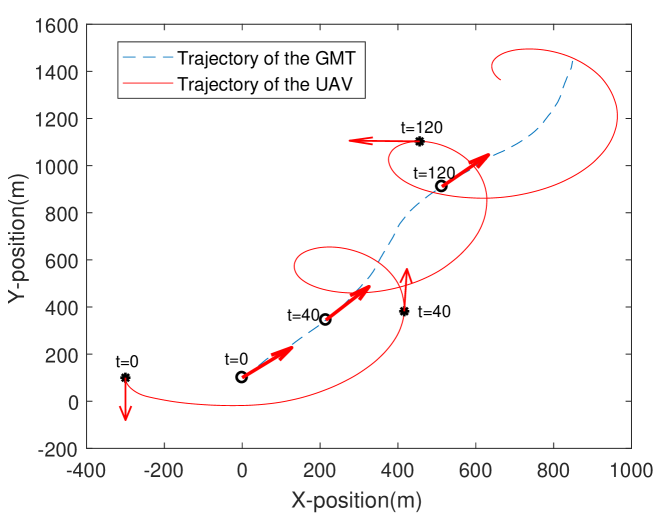
Figure 6: Trajectories of the GMT and the UAV in the X-Y plane.

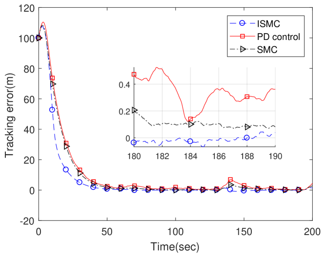
Figure 7: Tracking errors under different control methods.

In this subsection, we assume that the state of the GMT is known to the UAV. Since the guidance vectors in (11) can only be given online, i.e., guidance vectors after time $k$ are unavailable to the design of the $k$-th time input of the UAV, more advanced controllers do not always work, e.g., the model predictive control cannot be applied here as it relies on future guidance vectors [19]. Thus, we only compare the proposed ISMC with the PID control [5, 12, 1], and the standard SMC [38] for the UAV with dynamics in (4). The trajectories of the UAV and GMT are shown in Fig. 6, where circles and stars represent their positions at different time instants, and arrows denote course directions. The desired distance from the UAV to the GMT is set to $200$$\mathrm{m}$.

The comparison is depicted in Fig. 7, which shows that the proposed ISMC has the shortest setting time with zero steady-state error. We shall further test its effectiveness by using the estimated states via the RBPF.

VI-C Motion Estimation

In this section, we only test the estimation performance of the proposed RBPF. If the transition probability matrix $P$ in (3) for the maneuver process is unknown, each element of $P$ is set to $1/3$. Moreover, we adopt the Monte Carlo method by independently repeating $1000$ experiments to compute the root-mean-square error (RMSE) of the state estimate of the GMT, i.e.,

$$\text{RMSE}_{k}:=\left(\mathbb{E}[(\widehat{x}_{k}^{t}-{x}_{k}^{t})^{2}+(\widehat{y}_{k}^{t}-{y}_{k}^{t})^{2}]\right)^{1/2},$$ (42)

where $[\widehat{x}_{k}^{t},\widehat{y}_{k}^{t}]^{T}$ is produced by the RBPF. All simulations are of the same start position with $100$ particles in the RBPF.

For comparison, an EKF is also designed for the motion estimation. Note that the EKF requires the input to the GMT, which is unfortunately unknown in our setting. To solve it, we observe that the stationary distribution of the Markov chain under the transition probability matrix $P$ in (3) is a uniform distribution. Thus, we randomly sample a control input from the set $\{\bm{u}^{t}(1),\bm{u}^{t}(2),\bm{u}^{t}(3)\}$ with equal probability for the EKF.

VI-C1 Camera Sensor

TABLE I: Parameters of the ISMC

	$W$	$M$	$C$
v	0.2	5.0	5.0
$\psi$	0.04	0.6	3.0

The sampling frequency of the camera sensor is $25$$\mathrm{H}\mathrm{z}$ and the measurement noise is Gaussian white noise with covariance $R^{c}=\rm{diag}(0.03^{2},0.03^{2})$. Note that these parameters in real experiments of [5] are set as $30$$\mathrm{H}\mathrm{z}$ and $\rm{diag}(0.02^{2},0.02^{2})$, respectively. Fig. 8 illustrates the RMSE of the RBPF and EKF. One can observe that the performance of the RBPF is better than that of the EKF and is not significantly degraded even if the transition probability matrix $P$ is unknown, and both cases return favorable estimation performance.

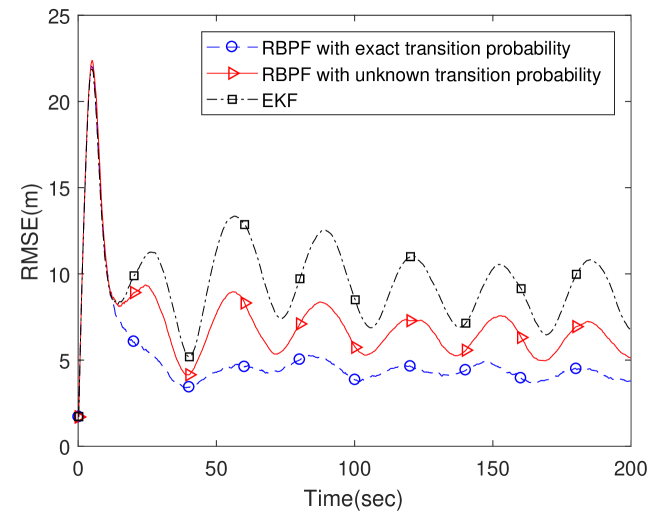
Figure 8: RMSE of the RBPF and EKF with a camera sensor.

VI-C2 Radar Sensor

For a radar sensor, we follow the same setting in [39] where the sampling frequency is $10$$\mathrm{H}\mathrm{z}$ and the covariance is $R^{r}=\rm{diag}(2.0^{2},0.01^{2})$. From Fig. 9, the same conclusion can be made as in the case of the camera sensor.

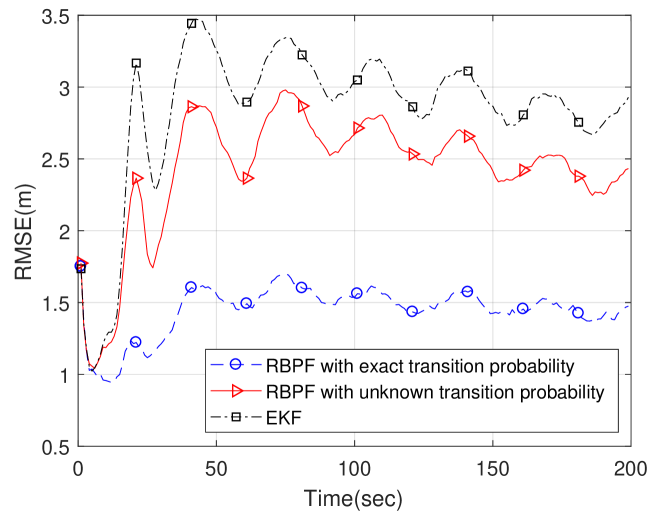
Figure 9: RMSE of the RBPF and EKF with a radar sensor.

Thus, both cases consistently verify the effectiveness of the RBPF.

VI-D Loitering Performance with Estimated States of the GMT

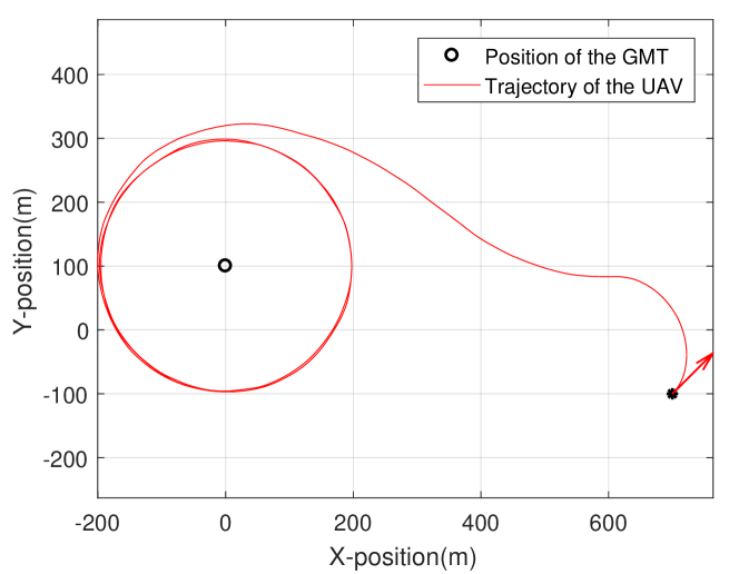
Figure 10: Trajectory of the UAV when the GMT is stationary.

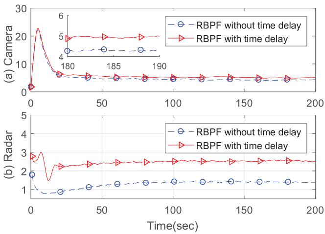
Figure 11: RMSE of the RBPF with: (a) a camera sensor; (b) a radar sensor.

In this subsection, we test the loitering performance of the UAV with estimated states of the GMT in (2). The sampling frequencies are of the same as that in Section VI-C with the consideration of $0.1$$\mathrm{s}$ time delay in sensor measurements. Note that the number of particles is still $100$.

Firstly, we consider the dynamics of the UAV in (4). When the GMT is stationary, Fig. 10 depicts the trajectory of the UAV under the proposed controller. Clearly, the UAV finally circumnavigates the GMT with a desired radius $200$$\mathrm{m}$.

Then, $\{\gamma_{k}\}$ is modeled as a nine state Markov chain, which corresponds to nine modes of maneuver: $\bm{u}^{t}(1)=[0,0]^{T}$, $\bm{u}^{t}(2)=[1,0]^{T}$, $\bm{u}^{t}(3)=[1,1]^{T}$, $\bm{u}^{t}(4)=[0,1]^{T}$, $\bm{u}^{t}(5)=[-1,1]^{T}$, $\bm{u}^{t}(6)=[-1,0]^{T}$, $\bm{u}^{t}(7)=[-1,-1]^{T}$, $\bm{u}^{t}(8)=[0,-1]^{T}$, $\bm{u}^{t}(9)=[1,-1]^{T}$. Moreover, all the diagonal elements of the transition probability matrix $P$ are $0.6$ and other elements are set to $0.05$. For the implementation of the RBPF, $P$ is assumed to be unknown and each element is simply set as $1/9$. Fig. 11 shows the RMSE defined in (42) over $1000$ times under different sensors.

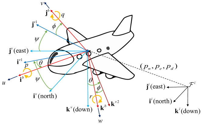
Figure 12: 6-DOF fixed-wing UAV and its associated coordinate frames [40].

Then, a 6-DOF fixed-wing UAV [40] is adopted to test the effectiveness of the proposed flight controller, see Fig. 12 where $[p_{n},p_{e},p_{d}]^{T}$ and $[\phi,\theta,\psi]^{T}$ are the position and orientation of the UAV in the inertial coordinate frame, respectively. $[u,v,w]^{T}$ and $[p,q,r]^{T}$ are linear velocities and angular rates in the body frame. Due to page limitation, we omit details of the mathematical model of the UAV, which can be found in [40], and adopt codes from [41] for the model. To complete the loitering task with a camera sensor, we design the controller by the proposed method of this work. The 3D trajectories of the GMT and the UAV are shown in Fig. 13, where the altitude is controlled to $100$$\mathrm{m}$ under the altitude controller in [41]. Moreover, the trajectories on X-Y plane, the trajectory in Z direction, the estimation error, and tracking error of one run are all depicted in Fig. 14. Simulation results in this case also indicate that the proposed flight controller is effective.

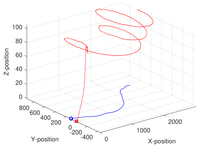
Figure 13: 3D trajectories of the GMT and the UAV.

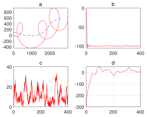
Figure 14: Simulation results: (a) trajectories of the GMT and the UAV projected in XY plane; (b) the altitude trajectory of the UAV; (c) the absolute estimation error of the GMT in one run; (d) the tracking error in one run.

VII Conclusion

In this paper, we proposed a discrete-time ISMC for the UAV to loiter over a GMT with three possible maneuvering states. To achieve it, a discrete-time guidance vector field was designed by assuming that the motion state of the GMT is known. Then, we designed a RBPF to simultaneously estimate the maneuver and the motion state of the GMT by using the measurements of a vision camera or a radar. Simulations finally validated our theoretical results.

References

• [1] M. Zhang and H. H. T. Liu, “Vision-based tracking and estimation of ground moving target using unmanned aerial vehicle,” in American Control Conference, 2010, pp. 6968–6973.
• [2] X. C. Ding, A. R. Rahmani, and M. Egerstedt, “Multi-UAV convoy protection: An optimal approach to path planning and coordination,” IEEE Transactions on Robotics, vol. 26, no. 2, pp. 256–268, 2010.
• [3] T. Oliveira, A. P. Aguiar, and P. Encarnação, “Moving path following for unmanned aerial vehicles with applications to single and multiple target tracking problems,” IEEE Transactions on Robotics, vol. 32, no. 5, pp. 1062–1078, 2016.
• [4] W. Meng, Z. He, R. Su, P. K. Yadav, R. Teo, and L. Xie, “Decentralized multi-UAV flight autonomy for moving convoys search and track,” IEEE Transactions on Control Systems Technology, vol. 25, no. 4, pp. 1480–1487, 2017.
• [5] V. N. Dobrokhodov, I. I. Kaminer, K. D. Jones, and R. Ghabcheloo, “Vision-based tracking and motion estimation for moving targets using unmanned air vehicles,” Journal of Guidance Control & Dynamics, vol. 31, no. 4, pp. 907–917, 2008.
• [6] E. W. Frew, D. A. Lawrence, C. Dixon, J. Elston, and W. J. Pisano, “Lyapunov guidance vector fields for unmanned aircraft applications,” in American Control Conference, 2007, pp. 371–376.
• [7] Z. Li, N. Hovakimyan, V. Dobrokhodov, and I. Kaminer, “Vision-based target tracking and motion estimation using a small UAV,” in IEEE Conference on Decision and Control, 2011, pp. 2505–2510.
• [8] T. Summers, M. Akella, and M. Mears, “Coordinated standoff tracking of moving targets: Control laws and information architectures,” Journal of Guidance Control & Dynamics, vol. 32, no. 1, pp. 56–69, 2009.
• [9] Y. Pan, X. Li, and H. Yu, “Efficient PID tracking control of robotic manipulators driven by compliant actuators,” IEEE Transactions on Control Systems Technology, vol. PP, no. 99, pp. 1–8, 2018.
• [10] Y. A. Kapitanyuk, A. V. Proskurnikov, and C. Ming, “A guiding vector-field algorithm for path-following control of nonholonomic mobile robots,” IEEE Transactions on Control Systems Technology, vol. PP, no. 99, pp. 1–14, 2017.
• [11] A. Loria, J. Dasdemir, and N. A. Jarquin, “Leader-follower formation and tracking control of mobile robots along straight paths,” IEEE Transactions on Control Systems Technology, vol. 24, no. 2, pp. 727–732, 2016.
• [12] E. W. Frew, D. A. Lawrence, and M. Steve, “Coordinated standoff tracking of moving targets using Lyapunov guidance vector fields,” Journal of Guidance Control & Dynamics, vol. 31, no. 2, pp. 290–306, 2008.
• [13] X. Yu and L. Liu, “Target enclosing and trajectory tracking for a mobile robot with input disturbances,” IEEE Control Systems Letters, vol. 1, no. 2, pp. 221–226, 2017.
• [14] M. Zhang and H. H. Liu, “Tracking a moving target by a fixed-wing UAV based on sliding mode control,” in AIAA Guidance, Navigation, and Control, 2013.
• [15] D. Chwa, “Sliding-mode tracking control of nonholonomic wheeled mobile robots in polar coordinates,” IEEE Transactions on Control Systems Technology, vol. 12, no. 4, pp. 637–644, 2004.
• [16] M. Z. Shah, R. Samar, and A. I. Bhatti, “Guidance of air vehicles: A sliding mode approach,” IEEE Transactions on Control Systems Technology, vol. 23, no. 1, pp. 231–244, 2015.
• [17] S. Sarpturk, Y. Istefanopulos, and O. Kaynak, “On the stability of discrete-time sliding mode control systems,” IEEE Transactions on Automatic Control, vol. 32, no. 10, pp. 930–932, 1987.
• [18] M. C. Saaj, B. Bandyopadhyay, and H. Unbehauen, “A new algorithm for discrete-time sliding-mode control using fast output sampling feedback,” IEEE Transactions on Industrial Electronics, vol. 49, no. 3, pp. 518–523, 2002.
• [19] E. F. Camacho and C. Bordons, Model predictive control.   Springer London, 2004.
• [20] J. Ghommam, N. Fethalla, and M. Saad, “Quadrotor circumnavigation of an unknown moving target using camera vision-based measurements,” Iet Control Theory & Applications, vol. 10, no. 15, pp. 1874–1887, 2016.
• [21] X. R. Li and V. P. Jilkov, “Survey of maneuvering target tracking. Part I. Dynamic models,” IEEE Transactions on Aerospace & Electronic Systems, vol. 39, no. 4, pp. 1333–1364, 2004.
• [22] J. Zhang, K. You, and L. Xie, “Bayesian filtering with unknown sensor measurement losses,” IEEE Transactions on Control of Network Systems, vol. 6, no. 1, pp. 163–175, 2019.
• [23] A. Doucet, N. De Freitas, and N. Gordon, “An introduction to sequential Monte Carlo methods,” in Sequential Monte Carlo Methods in Practice.   Springer, 2001, pp. 3–14.
• [24] A. Doucet, N. De Freitas, K. Murphy, and S. Russell, “Rao-Blackwellised particle filtering for dynamic Bayesian networks,” in Proceedings of the Sixteenth Conference on Uncertainty in Artificial Intelligence.   Morgan Kaufmann Publishers Inc., 2000, pp. 176–183.
• [25] F. Gustafsson, F. Gunnarsson, N. Bergman, and U. Forssell, “Particle filters for positioning, navigation and tracking,” IEEE Transactions on Signal Processing, vol. 50, no. 2, pp. 425–437, 2002.
• [26] F. Dong, J. Zhang, and K. You, “Maneuvering target tracking and motion estimation using vision-aid particle filter,” in the 43rd Annual Conference of the IEEE Industrial Electronics Society, 2017, pp. 6733–6738.
• [27] D. P. Bertsekas, Dynamic programming and optimal control.   Athena scientific Belmont, MA, 1995, vol. 1, no. 2.
• [28] S. J. Liu and P. P. Zhang, “Discrete-time stochastic source seeking via tuning of forward velocity,” IFAC Papersonline, vol. 48, no. 28, pp. 927–932, 2015.
• [29] W. Ren and R. W. Beard, “Trajectory tracking for unmanned air vehicles with velocity and heading rate constraints,” IEEE Transactions on Control Systems Technology, vol. 12, no. 5, pp. 706–716, 2004.
• [30] Y. Kang and J. K. Hedrick, “Linear tracking for a fixed-wing UAV using nonlinear model predictive control,” IEEE Transactions on Control Systems Technology, vol. 17, no. 5, pp. 1202–1210, 2009.
• [31] R. W. Beard, J. Ferrin, and J. Humpherys, “Fixed wing UAV path following in wind with input constraints,” IEEE Transactions on Control Systems Technology, vol. 22, no. 6, pp. 2103–2117, 2014.
• [32] F. Dong, X. Lei, and W. Chou, “A dynamic model and control method for a two-axis inertially stabilized platform,” IEEE Transactions on Industrial Electronics, vol. 64, no. 1, pp. 432–439, 2017.
• [33] D. Lawrence, “Lyapunov vector fields for UAV flock coordination,” in 2nd AIAA Unmanned Unlimited Conference, Workshop, and Exhibit, 2003.
• [34] H. K. Khalil, Nonlinear Systems (3rd Ed.).   Prentice Hall, 2002.
• [35] H. Du, X. Yu, M. Z. Q. Chen, and S. Li, “Chattering-free discrete-time sliding mode control,” Automatica, vol. 68, no. C, pp. 87–91, 2016.
• [36] M. S. Arulampalam, S. Maskell, N. Gordon, and T. Clapp, “A tutorial on particle filters for online nonlinear/non-gaussian Bayesian tracking,” IEEE Transactions on Signal Processing, vol. 50, no. 2, pp. 174–188, 2002.
• [37] B. D. Anderson and J. B. Moore, Optimal Filtering.   Dover Publications, 2005.
• [38] W. Perruquetti and J. P. Barbot, “Sliding mode control in engineering,” Dekker, pp. 53–101, 2002.
• [39] A. Averbuch, S. Itzikowitz, and T. Kapon, “Radar target tracking-viterbi versus imm,” Aerospace & Electronic Systems IEEE Transactions on, vol. 27, no. 3, pp. 550–563, 1991.
• [40] R. W. Beard and T. W. Mclain, Small Unmanned Aircraft: Theory and Practice.   Princeton University Press, 2012.
• [41] J. Lee, https://github.com/magiccjae/ecen674.