Fitting formulae for evolution tracks of massive stars under extreme metal poor environments for population synthesis calculations and star cluster simulations

Abstract

We have devised fitting formulae for evolution tracks of massive stars with $8\lesssim M/M_{\odot}\lesssim 160$ under extreme metal poor (EMP) environments for $\log(Z/Z_{\odot})=-2,-4,-5,-6$, and $-8$, where $M_{\odot}$ and $Z_{\odot}$ are the solar mass and metallicity, respectively. Our fitting formulae are based on reference stellar models which we have newly obtained by simulating the time evolutions of EMP stars. Our fitting formulae take into account stars ending with blue supergiant (BSG) stars, and stars skipping Hertzsprung gap (HG) phases and blue loops, which are characteristics of massive EMP stars. In our fitting formulae, stars may remain BSG stars when they finish their core Helium burning (CHeB) phases. Our fitting formulae are in good agreement with our stellar evolution models. We can use these fitting formulae on the SSE, BSE, NBODY4, and NBODY6 codes, which are widely used for population synthesis calculations and star cluster simulations. These fitting formulae should be useful to make theoretical templates of binary black holes formed under EMP environments.

1 Introduction

Laser Interferometer Gravitational-Wave Observatory (LIGO) has finally detected the first gravitational wave from a black hole (BH) merger (Abbott et al., 2016). Since then, many BH-BH mergers have been observed by gravitational wave observatories LIGO and VIRGO (e.g. Abbott et al., 2019). These detections have raised an important question: what the origin of these merging BH-BHs is. One of the promising origins is massive binary stars. However, it has been still under debate what stellar metallicity such massive binary stars have: Population (Pop.) I/II stars (e.g. Belczynski et al., 2016a) or Pop. III stars (e.g. Kinugawa et al., 2014), and where they are formed: galactic fields (e.g. Tutukov et al., 1973; Bethe & Brown, 1998) or star clusters (e.g. Portegies Zwart & McMillan, 2000). In order to elucidate the origin of these merging BH-BHs, one has to make theoretical templates of merging BH-BHs, and compare them with observed BH-BH populations.

Population synthesis calculations and star cluster simulations are powerful tools to make such theoretical templates of merging BH-BHs from galactic fields and from star clusters, respectively. In either case, BH-BHs from Pop. I/II stars with $0.01\lesssim Z/Z_{\odot}\lesssim 1$ have been intensively studied so far (e.g. Belczynski et al., 2016a; Rodriguez et al., 2016), where $Z$ and $Z_{\odot}$ are metallicity and the solar metallicity, respectively. On the other hand, BH-BHs formed from extreme metal poor (EMP) stars with $Z/Z_{\odot}\lesssim 0.01$ (including Pop. III stars) have been not examined well.

Kinugawa et al. (2014) have found that Pop. III BH-BHs have distinct features from Pop. I/II BH-BHs by means of population synthesis calculations. The mass distribution of Pop. III BH-BHs have a much larger peak than those of Pop. I/II BH-BHs. This argument is insensitive to the choices of stellar initial mass functions (IMFs) and initial binary parameters (Kinugawa et al., 2016). Thus, Pop. III BH-BHs can have significant contribution to observed BH-BHs. Inayoshi et al. (2017) have confirmed their arguments by simulating Pop. III star evolutions. The reason for this difference comes from stability of mass transfer of BH-BH progenitors. Massive Pop. I/II stars become red supergiant (RSG) stars, and have convective envelopes after a certain time in their lives. Such stars easily experience unstable mass transfer or common envelope evolution (Paczynski, 1976; Iben & Livio, 1993; Taam & Sandquist, 2000; Ivanova et al., 2013), just after they begin Roche-lobe overflow. In fact, most of BH-BH progenitors experience common envelope evolution for Pop. I/II stars (e.g. Bethe & Brown, 1998; Belczynski et al., 2002; Dominik et al., 2012, 2013; Mennekens & Vanbeveren, 2014; Belczynski et al., 2014; Spera et al., 2015; Eldridge & Stanway, 2016; Belczynski et al., 2016a; Eldridge et al., 2017; Mapelli et al., 2017; Stevenson et al., 2017; Mapelli & Giacobbo, 2018; Giacobbo & Mapelli, 2018; Kruckow et al., 2018; Spera et al., 2019; Mapelli et al., 2019; Eldridge et al., 2019). On the other hand, a significant fraction of massive Pop. III stars end with blue supergiant (BSG) stars which have radiative envelopes, since they have small opacities (e.g. Marigo et al., 2001; Ekström et al., 2008). They tend to undergo stable mass transfer when they interact with their companion stars. Such stable mass transfer loses less stellar masses than common envelope evolution for the following reason. If neither of two stars are white dwarfs, neutron stars (NSs), and BHs, their total mass is nearly conservative in stable mass transfer, while they can lose all their envelopes in common envelope evolution as back reaction of the tightening of the binary orbit. Hence, Pop. III BH-BHs can be more massive than Pop. I/II BH-BHs.

Moreover, Pop. III stars should have a different formation mode from Pop. I/II stars. Pop. I/II stars have typical mass of $\sim 1M_{\odot}$ at the formation time, and top-light IMFs (Salpeter, 1955; Kroupa, 2001). On the other hand, the typical mass of Pop. III stars should be $10$ – $1000M_{\odot}$ at the initial time, and their IMF should be top-heavy (Omukai & Nishi, 1998; Abel et al., 2002; Bromm & Larson, 2004; Yoshida et al., 2008; Hosokawa et al., 2011; Stacy et al., 2011, 2012; Bromm, 2013; Susa, 2013; Susa et al., 2014; Hirano et al., 2015). The formation mode may transition from Pop. I/II like to Pop. III like at $Z/Z_{\odot}\sim 10^{-3}$ - $10^{-6}$ (Bromm & Loeb, 2003; Omukai et al., 2005; Schneider et al., 2006; Maio et al., 2010). IMFs will be an important factor to amplify the difference between Pop. I/II and Pop. III BH-BHs. We again emphasize that the typical masses of Pop. III BH-BHs in Kinugawa et al. (2014) are mostly unchanged even if the top-heavy IMF is changed to Pop. I/II IMFs.

Since Pop. III BH-BHs have distinct features from Pop. I/II BH-BHs, it is instructive to bridge the metallicity gap between Pop. I/II and Pop. III stars, and make templates of BH-BHs originating from EMP stars with $0\lesssim Z/Z_{\odot}\lesssim 0.01$. Such templates can constrain the dominant metal environments under which BH-BH progenitors are formed. Even if Pop. III and EMP environments are not dominant (Hartwig et al., 2016; Belczynski et al., 2017), such templates will help surveying Pop. III BH-BHs from an enormous number of merging BH-BHs in current and future gravitational wave observations (Nakamura et al., 2016). The direct detection of Pop. III stars and their remnants have neither yet succeeded for massive and short-lived Pop. III stars (Rydberg et al., 2013), nor for low-mass and long-lived Pop. III stars (Frebel & Norris, 2015), although the latter Pop. III stars might be observed as metal-enriched stars due to metal pollution by interstellar gas, dust, and asteroids (Komiya et al., 2015; Johnson, 2015; Tanikawa et al., 2018; Kirihara et al., 2019).

In this paper, we devise evolution tracks of massive EMP stars for population synthesis calculations and star cluster simulations, based on stellar evolution simulations for massive stars with $8\leq M/M_{\odot}\leq 160$, where $M$ and $M_{\odot}$ are stellar mass and the solar mass. There are many evolution tracks: SSE and BSE (Hurley et al., 2000, 2002), SeBa (Portegies Zwart & Verbunt, 1996), Scenario Machine (Lipunov et al., 1996), StarTrack (Belczynski et al., 2002), and BINARY_C, (Izzard et al., 2018) driven by fitting formulae, and SEVN (Spera et al., 2015; Spera et al., 2019), BPASS (Eldridge & Stanway, 2016), and COMBINE (Kruckow et al., 2018) based on detailed evolutionary models. However, these evolution tracks support Pop. I/II stars with $0.001\lesssim Z/Z_{\odot}\lesssim 1$. Kinugawa et al. (2014) have supported evolution tracks of just Pop. III stars (i.e. $Z/Z_{\odot}=0$), based on the model of Marigo et al. (2001). Our evolution tracks support EMP stars with $Z/Z_{\odot}=10^{-2},10^{-4},10^{-5},10^{-6}$, and $10^{-8}$, and bridge the metallicity gap. For EMP stars, the evolution tracks of $Z=10^{-4},10^{-6},10^{-10}$ and $0.7\leq M\leq 15M_{\odot}$ stars have been investigated (Cassisi & Castellani, 1993). The metallicity dependence of 20 $M_{\odot}$ stars with $Z=10^{-8},10^{-5},0.02$ have been investigated in Hirschi (2007). However, no systematic studies of the evolution tracks for EMP massive stars have been performed.

We preferentially make evolution tracks of massive EMP stars, since stars should be dominantly formed as massive stars in EMP environments. However, we will make evolution tracks of low-mass EMP stars in near future. Many studies have claimed that low-mass stars could be formed even under metal-free environments (Nakamura & Umemura, 2001; Machida et al., 2008; Clark et al., 2011b, a; Greif et al., 2011, 2012; Machida & Doi, 2013; Susa et al., 2014; Chiaki et al., 2016; Susa, 2019).

We have developed our evolution tracks as forms of fitting formulae in order to incorporate the evolution tracks into SSE  (Hurley et al., 2000), BSE (Hurley et al., 2002), and NBODY4 and NBODY6 (Aarseth, 2003; Nitadori & Aarseth, 2012; Wang et al., 2015). Several population synthesis calculation codes (e.g. Belczynski et al., 2002; Kinugawa et al., 2014; Giacobbo & Mapelli, 2018) are based on the BSE code. The NBODY4 and NBODY6 codes are widely used to derive BH-BH populations originating from star clusters (e.g. Banerjee et al., 2010; Tanikawa, 2013; Bae et al., 2014; Banerjee, 2017; Fujii et al., 2017; Park et al., 2017; Hong et al., 2018; Kumamoto et al., 2019; Di Carlo et al., 2019b; Di Carlo et al., 2019a). Moreover, many works have obtained BH-BH populations formed in star clusters, using star cluster simulation codes coupled with the BSE code (e.g. Giersz et al., 2013; Rodriguez et al., 2018). Therefore, we believe that our evolution tracks can be used on many codes for population synthesis calculations and star cluster simulations with minor adjustments.

The structure of this paper is as follows. In section 2, we overview our evolution models of EMP stars as reference models of our evolution tracks. In section 3, we describe how to make the fitting formulae for the evolution tracks of EMP stars. In section 4, we compare our fitting formulae with our stellar evolution models. In section 5, we summarize this paper. The units of time, luminosity, radius, and mass are Myr, $L_{\odot}$ (the solar luminosity), $R_{\odot}$ (the solar radius), and $M_{\odot}$, respectively, if otherwise specified.

2 Stellar evolution models

We need stellar evolution models as reference, in order to make fitting formulae. We present our simulation method to make the stellar evolution models in section 2.1. In section 2.2, we overview our stellar evolution models.

2.1 Simulation method

Our simulation method is similar to 1 dimensional (1D) simulation method in Yoshida et al. (2019). We follow the time evolutions of stars with $M=$ 8, 10, 13, 16, 20, 25, 32, 40, 50, 65, 80, 100, 125, and 160 $M_{\odot}$ for $\log(Z/Z_{\odot})$ = -2, -4, -5, -6 and $-8$ from the zero age main-sequence (ZAMS) to the carbon ignitions at the stellar centers. We use a 1D stellar evolution code, HOSHI code (Takahashi et al., 2016, 2018, 2019; Yoshida et al., 2019). Here we describe some details for the chemical mixing by convection and input physics in the stellar evolution model. We do not account for rotation and rotational mixing.

We adopt the Ledoux criterion for convective instability, and model chemical mixing in a convective region by means of the mixing length theory with diffusion coefficients as described in Takahashi et al. (2019). The diffusion coefficient in the convective region is described as

$$D_{\rm cv}=\frac{1}{3}v_{\rm mix}l_{\rm mix},$$ (1)

where $v_{\rm mix}$ is the velocity of convective blobs, $l_{\rm mix}=\alpha_{\rm mix}H_{P}$ is the mixing length, and $H_{P}$ is the pressure scale height. The velocity of convective blobs is determined by the mixing length theory (Böhm-Vitense, 1958). The mixing length parameter $\alpha_{\rm mix}$ is set to be 1.8. In semiconvection region, we model diffusive chemical mixing with the diffusion coefficient derived in Spruit (1992),

$$D_{\rm sc}=f_{\rm sc}\frac{\nabla_{\rm rad}-\nabla_{\rm ad}}{(\varphi/\delta)\nabla_{\mu}}D_{{\rm therm}},$$ (2)

where $f_{\rm sc}$ is a parameter corresponding to the square root of the ratio of solute diffusivity to thermal diffusivity, $\nabla_{\rm rad}\equiv(\kappa L/16\pi cGM_{r})(3P/aT^{4})$ is a radiative gradient, $\kappa$ is opacity, $L$ is luminosity, $c$ is the speed of light, $G$ is the gravitational constant, $M_{r}$ is the mass coordinate, $P$ is pressure, $a$ is the radiation constant, $T$ is temperature, $\nabla_{\rm ad}\equiv(\partial\ln T/\partial\ln P)_{s,\mu}$ is an adiabatic gradient, $s$ is entropy, $\mu$ is mean molecular weight, $\nabla_{\mu}\equiv d\ln\mu/d\ln P$ is a spatial gradient of mean molecular weight and $P$ is taken as a measure of depth, $\varphi\equiv(\partial\ln\rho/\partial\ln\mu)_{P,T}$ and $\delta\equiv-(\partial\ln\rho/\partial\ln T)_{P,\mu}$ are thermodynamic derivatives, $\rho$ is density, thus $\varphi/\delta=(\partial\ln T/\partial\ln\mu)_{P,\rho}$, $D_{\rm therm}=4acT^{3}/3\kappa C_{P}$ is the thermal diffusivity, $C_{P}$ is the specific heat by unit mass at constant pressure (e.g. Kippenhahn & Weigert, 1990; Maeder, 2009). The parameter $f_{\rm sc}$ is set to be 0.3, which is the same value in Takahashi et al. (2019) (see also Umeda et al., 1999; Umeda & Nomoto, 2008).

We also take into account chemical mixing by convective overshoot as a diffusive process above convective regions. The diffusion coefficient of the overshoot chemical mixing exponentially decreases with the distance from the convective boundary as

$$D^{\rm ov}_{\rm cv}=D_{\rm cv,0}\exp\left(-2\frac{\Delta r}{f_{\rm ov}H_{P0}}\right),$$ (3)

where $D_{\rm cv,0}$ and $H_{P0}$ are the diffusion coefficient and the pressure scale height at the convective boundary, respectively, and $\Delta r$ is the distance from the boundary. The overshoot parameter $f_{\rm ov}$ is set to be 0.03, which is the same as the value of Set L_A in Yoshida et al. (2019). This overshoot parameter is determined based on the calculation to early-B type stars in the Large Magellanic Cloud similarly to Stern model (Brott et al., 2011). The main-sequence width of a solar-metallicity 20 $M_{\odot}$ model is almost same as that of the corresponding Stern model (see Fig. 12 ($a$) in Yoshida et al., 2019).

For nuclear reaction network, 49 species of nuclei are taken into account throughout evolution calculations. We include thermonuclear reactions and weak interactions ($\beta$ decays and electron captures) concerning to the nuclear species, so the evolution calculation from hydrogen burning (pp-chain and CNO cycles) until core-collapse (Si burning and photo-disintegration) is available. The rates of thermonuclear reactions are adopted from JINA REACLIB v1 (Cyburt et al., 2010) except for ¹²C($\alpha,\gamma)^{16}$C. The rate of ¹²C($\alpha,\gamma)^{16}$O is adopted from Caughlan & Fowler (1988) and is multiplied by a factor of 1.2 (Takahashi et al., 2018).

We derive the initial composition of massive stars with a given metallicity from the mixture of the solar-system composition and the primordial chemical composition. The elemental composition of the solar system is evaluated from the bulk composition of the Sun in Asplund et al. (2009). The mass fractions of hydrogen, helium, and heavier elements are $X=0.7155$, $Y=0.2704$, and $Z=0.0141$, respectively. The isotopic ratio of each element is taken from the table of the solar-system abundance derived from meteoritic and solar photosphere data in Lodders et al. (2009). The primordial chemical composition is adopted from Eqs. (22)–(25) in Steigman (2007). EMP stars do not necessarily have chemical abundance scaled down from the solar-system abundance (see Frebel & Norris, 2015, for review). However, there is no conclusive abundance pattern for EMP stars. Thus, we adopt the scaling down of the solar-system abundance conservatively.

We use the equation of state of Blinnikov et al. (1996), which includes the effects of electrons, positrons, ions, and photons. In low temperature and density region, we use a non-degenerate equation of state for electrons, ions, atoms, molecules, and photons taking account of partial ionization and molecular dissociation (Vardya, 1960; Iben, 1963). We evaluate opacity using tables of OPAL opacity (Iglesias & Rogers, 1996), molecular opacity (Ferguson et al., 2005), and conductive opacity (Cassisi et al., 2007). We evaluate the energy loss by neutrinos using approximation formula in Itoh et al. (1996).

We have to extract data of He and CO core masses from the simulation results. For this purpose, we define the He and CO cores of stars as follows. The He-core mass is determined as the mass coordinates at the outermost region where the hydrogen mass fraction is less than 0.1. The CO-core mass is determined as the mass coordinates at the outermost region where the helium mass fraction is less than 0.1.

We do not include stellar wind mass loss in our simulations, since we usually consider stellar wind mass loss while following fitting formulae in population synthesis calculations and star cluster simulations (e.g. Hurley et al., 2000).

We stop following stellar evolutions when carbon is ignited at the stellar centers. We can take into account the post-carbon burning evolutions by a post-processing way in population synthesis calculations and star cluster simulations. This is because stars evolve on small timescale after the carbon ignition. We confirmed that the expansion of the radius from the carbon burning until the onset of the core collapse (when the central temperature reaches $10^{9.9}$ K) is less than 2 % in a BSG star of $M/M_{\odot}=13M_{\odot}$ and $\log(Z/Z_{\odot})=-8$. As a demonstration, we implement the post-carbon burning evolutions, such as effects of core-collapse supernova (SN) explosion, pulsational pair instability (PPI) before core-collapse SN explosion, and pair instability (PI) SNe, in section 3.5.

Our stellar models have masses of $\leq 160M_{\odot}$, smaller than possible Pop. III masses ($\gtrsim 200M_{\odot}$). Nevertheless, this mass range should be sufficient for our purpose for the following reason. Pop. III stars are formed in protostellar clouds with $\sim 1000M_{\odot}$ (e.g. Yoshida et al., 2003). The protostellar clouds are gravitationally fragmented, and a large part of the protostellar clouds are ejected through star forming processes, according to recent numerical simulations (see Dayal & Ferrara, 2018, for a review). Therefore, Pop. III stars with $\gtrsim 200M_{\odot}$ should not be typical, and should be single if present. The evolutions of single massive Pop. III stars must be interesting, however stellar models with masses of $\leq 160M_{\odot}$ should be enough to investigate BH-BH merger events currently observed.

2.2 Simulation results

We briefly review the evolutions of massive Pop. I/II stars including stars with $\log(Z/Z_{\odot})=-2$ before we see the simulation results. A star starts from a main-sequence (MS) phase in which hydrogen is burned at the center of the star. The beginning time of the MS is called the ZAMS time. When hydrogen is burned out at the center, a helium (He) core has been formed inside of the star. Then, the He core and its hydrogen envelope shrink, which is called a hook phase. The hook phase ends with hydrogen ignition on the surface of the He core, and is followed by a Hertzsprung gap (HG) phase in which the He core continues to shrink while the hydrogen envelope begins expanding. At some point, helium is ignited in the He core, and a core helium burning (CHeB) phase starts. In general, a massive star never becomes a red giant branch (RGB) star before entering into a CHeB phase. In the CHeB phase, the stellar envelope transiently shrinks and expands again, if the star is relatively light. This behavior is called a blue loop. The stellar envelope monotonically expands if the star is relatively heavy. The CHeB phase finishes when helium is completely converted to carbon and oxygen (CO) at the center, and the CO core emerges at the center. Subsequently, helium keeps burned on the surface of the CO core. Thus, this phase is called a shell helium burning (ShHeB) phase. The star becomes a RSG star in either of the CHeB or ShHeB phase. The ShHeB phase continues until carbon is ignited at the center. Shortly after the carbon ignition, the star experiences a SN explosion, or gravitational collapse. Then, it finally leaves a NS or BH.

There are three different points between Pop. I/II stars and EMP stars (including Pop. III stars). (1) Some of EMP stars never become RSG stars. (2) EMP stars experience smaller blue loops than Pop. I/II stars, and a part of EMP stars have no blue loops. (3) A part of EMP stars skip HG phases. These points will be described in detail below.

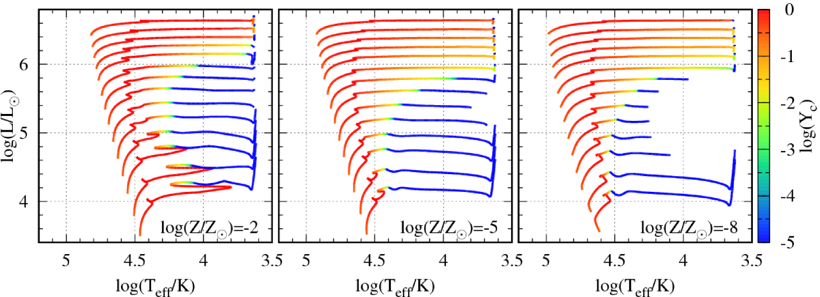
Figure 1: HR diagrams for stellar models with $\log(Z/Z_{\odot})=-2,-5$, and $-8$. In each panel, curves indicate stellar evolutions with $M/M_{\odot}=8,10,13,16,20,25,32,40,50,65,80,100,125$, and $160$ from bottom to top. Colors are coded by the helium mass fractions in the stellar cores.

Figure 1 shows Hertzsprung-Russell (HR) diagrams for different metallicities. All the stars become RSG stars with $\log(T_{\rm eff}/\mbox{K})\lesssim 3.7$ for $\log(Z/Z_{\odot})=-2$, while some of stars end with BSG stars with $\log(T_{\rm eff}/\mbox{K})\gtrsim 3.7$ for $\log(Z/Z_{\odot})=-5$ and $-8$. The mass range of stars ending with BSG stars becomes wider with metallicity decreasing: $20\lesssim M/M_{\odot}\lesssim 32$ for $\log(Z/Z_{\odot})=-5$, and $13\lesssim M/M_{\odot}\lesssim 40$ for $\log(Z/Z_{\odot})=-8$. This is because stars have smaller opacity as they become more metal-poor. Global features of the HR diagram are not changed when the resolution of the evolution calculation is increased. The time evolution of surface temperature between HG and RSG phases and the variation of luminosity in RSG phase are slightly affected by the resolution in some cases.

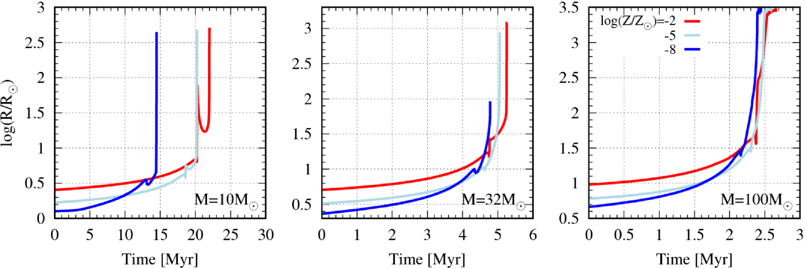
Figure 2: Radius evolutions of stars with $M/M_{\odot}=10$, $32$, and $100$ for $\log(Z/Z_{\odot})=-2,-5$, and $-8$.

In Figure 1, we can see the absence of blue loops for EMP stars. For $\log(Z/Z_{\odot})=-2$, relatively light stars ($8\lesssim M/M_{\odot}\lesssim 25$) have blue loops. The $M=8M_{\odot}$ star has the most prominent one among them. Its effective temperature returns up to $\log(T_{\rm eff}/\mbox{K})\sim 4.3$ after its effective temperature decreases down to $\log(T_{\rm eff}/\mbox{K})\sim 3.8$ once. For $\log(Z/Z_{\odot})=-5$, stars with $8\lesssim M/M_{\odot}\lesssim 16$ still have blue loops, and however their blue loops are much less prominent than those of stars for $\log(Z/Z_{\odot})=-2$. Even for the $M=8M_{\odot}$ star, the beginning temperature of the blue loop is different from the highest temperature in the blue loop only by $\Delta\log(T_{\rm eff}/\mbox{K})\lesssim 0.1$. Finally, blue loops disappear from all the stars for $\log(Z/Z_{\odot})=-8$.

EMP stars may skip their HG phases. This can be seen in Figure 2 which shows the radius evolutions of stars with different masses and metallicities. For a star with $M=10M_{\odot}$ and $\log(Z/Z_{\odot})=-2$, its radius monotonically increases from $\log(R/R_{\odot})\sim 0.4$ to $\log(R/R_{\odot})\sim 0.8$ until $t\sim 20$ Myr in its MS phase, slightly decreases by $\Delta\log(R/R_{\odot})\sim 0.1$ in the hook phase, and increases by $\Delta\log(R/R_{\odot})\sim 1.1$ on a short timescale in the HG phase. We can see that the radius also increases by $\Delta\log(R/R_{\odot})\sim 0.2$ at $t\sim 18$ Myr in the HG phase for $\log(Z/Z_{\odot})=-5$. However, the increase of the radius for $\log(Z/Z_{\odot})=-5$ is much smaller than for $\log(Z/Z_{\odot})=-2$. Such radius increase is absent for $\log(Z/Z_{\odot})=-8$; the HG phase disappears for $\log(Z/Z_{\odot})=-8$. Although the stellar radius increases for $\log(Z/Z_{\odot})=-8$ at $t\sim 14$ Myr, the star have entered into the ShHeB phase at this time. From the above, we see the presence and absence of the HG phases for the case of $M=10M_{\odot}$. This can be true for the case of $M=32$ and $100M_{\odot}$ (see the middle and right panels of Figure 2). More metal-poor stars have higher temperature at their centers at their MS phases due to inefficiency of the CNO cycle. Then, their central temperature more easily exceeds the temperature of helium ignition during their hook phases. The dependence of the beginning time of CHeB phases is systematically discussed in Schootemeijer et al. (2019).

We should remark difference between Hurley’s model and our model for $\log(Z/Z_{\odot})=-2$. In Hurley’s model, which supports for $-2\lesssim\log(Z/Z_{\odot})\lesssim 0$, the stars always become RSG stars when their CHeB phases end. On the other hand, in our model, relatively light stars still remain BSG stars when their CHeB phases end. This can be seen in Figure 1. For $\log(Z/Z_{\odot})=-2$, stars with $M/M_{\odot}\lesssim 50$ still remain BSG stars even when their central helium mass fractions are decreased down to less than $10^{-5}$; they finish their CHeB phases.

In summary, our model has three different points from Hurley’s model due to lower metallicity. Some of EMP stars end with BSG stars, and skip HG and blue loop phases. There is one different point between Hurley’s and our model even for Pop. I/II stars ($\log(Z/Z_{\odot})=-2$). Stars in Hurley’s model necessarily become RSG stars when they finish their CHeB phases, while stars in our model may remain BSG stars when they finish their CHeB phases.

Finally, we compare our model of $\log(Z/Z_{\odot})=-8$ with a zero-metal model of Marigo et al. (2001). Here, we identify our model of $\log(Z/Z_{\odot})=-8$ with a zero-metal model. In our model, stars with $13\leq M/M_{\odot}\leq 40$ end with BSG stars, and stars with $M/M_{\odot}\leq 10$ or $M/M_{\odot}\geq 50$ end with RSG stars. Thus, the lower and upper mass limits of stars ending with BSG stars are $10<M/M_{\odot}\leq 13$ and $40<M/M_{\odot}\leq 50$, respectively. On the other hand, in Marigo’s model, the corresponding mass limits are $9.5<M/M_{\odot}\leq 10$ and $50<M/M_{\odot}\leq 70$, respectively. The mass range of stars ending with BSG stars in our model is in a good agreement with that in Marigo’s model, although our mass range is slightly smaller than Marigo’s.

3 Implementation

In this section, we show the way to devise fitting formulae for evolution tracks of massive EMP stars, using our stellar evolution models as reference. The fitting formulae consist of a luminosity, radius, and He core mass as functions of time ($t$), mass ($M$), and metallicity ($Z$). We never construct three variable functions for these quantities. Instead, we develop bivariate functions with different metallicity, $\log(Z/Z_{\odot})=-2,-4,-5,-6$ and $-8$. The bivariate functions have totally different forms among stellar evolution phases, since stars evolve differently among these phases. We divide a stellar evolution into five phases: MS, HG, CHeB, ShHeB, and remnant phases. Note that the MS phase includes a hook phase, and massive stars skip RGB phases. We construct a bivariate function for a stellar quantity for a given phase as follows. We make fitting formulae for the stellar quantities at the beginning and ending times of the phase as a function of $M$. We obtain the stellar quantity at a given time of the phase by a simple polynomial interpolation that bridges the stellar quantities at the beginning and ending times of the phase.

Table 1: Mass limits constraining stellar evolutions.

$\log(Z/Z_{\odot})$	$-2$	$-4$	$-5$	$-6$	$-8$
$M_{\rm HG,u}$	–	–	$25$	$10$	$8$
$M_{\rm BL,u}$	$32$	$32$	$20$	$10$	$8$
$M_{\rm EB,l}$	$25$	$25$	$20$	$16$	$13$
$M_{\rm EB,u}$	$25$	$25$	$40$	$50$	$50$
$M_{\rm CB,u}$	$100$	$50$	$50$	$50$	$50$

As described in section 2, the critical masses of stars experiencing HG phases and blue loops become smaller with metallicity decreasing. Moreover, the mass range of stars ending with BSG stars is extended with metallicity decreasing. We consider such metallicity dependences by defining five mass limits: the upper mass limit of stars entering into HG phases ($M_{\rm HG,u}$), the upper mass limit of stars with blue loops ($M_{\rm BL,u}$), the upper and lower mass limits of stars ending with BSG stars ($M_{\rm EB,u}$ and $M_{\rm EB,l}$, respectively), and the upper mass limit of stars remaining BSG stars in CHeB phases ($M_{\rm CB,u}$). Then, stars enter into HG phases if $M<M_{\rm HG,u}$, and have blue loops if $M<M_{\rm BL,u}$. We indicate $M_{\rm HG,u}$ as “–” for $\log(Z/Z_{\odot})=-2$ and $-4$, since all the stars enter into HG phases for these metallicities. Stars end with BSG stars if $M_{\rm EB,l}\leq M<M_{\rm EB,u}$. Stars remain BSG stars in their CHeB phases if $M<M_{\rm CB,u}$. We summarize these mass limits in Table 1.

We can categorize phases (MS, HG, CHeB, ShHeB, remnant (NS/BH), BSG, and RSG) into two types. The first type includes MS, HG, CHeB, ShHeB, and remnant phases, which indicate states of stellar cores. The second type contains BSG and RSG phases indicating stellar surfaces. The former and latter types of phases are not exclusive. For example, a star can be in CHeB and BSG phases. We summarize these phases in Table 2.

Table 2: Definitions of phases.

Phase	Definition
MS	Phase from core hydrogen ignition to shell hydrogen ignition
HG	Phase from shell hydrogen ignition to core He ignition
CHeB	Phase from core He ignition to the end of core He burning
ShHeB	Phase from the end of core He burning to the carbon ignition
Remnant	Phase in which a star do not evolve any more as a single star
BSG	Phase with $\log(T_{\rm eff}/\mbox{K})\geq 3.65$
RSG	Phase with $\log(T_{\rm eff}/\mbox{K})<3.65$

We need to define these phases numerically in order to extract these phases from our stellar evolution model, i.e. 1D simulation data. These definitions are so technical, since we treat wide ranges of stellar masses and metallicities. The definitions of the first type of phases are as follows.

• MS phase. It starts from the ZAMS time defined as the time when a duration passes after the beginning of 1D simulation. The duration is 2 times of the maximum Kelvin-Helmholtz (KH) time in 1D simulations. The maximum KH time is achieved around the beginning time of the simulation. We can avoid a contraction phase from the initial hydrostatic equilibrium to the core hydrogen ignition. The MS phase ends at the time when the radius achieves the first local minimum.

• HG phase. It starts from the ending time of the MS phase, and ends at the He ignition time.

• CHeB phase. It starts at the He ignition time. If a star does not have an HG phase ($M\geq M_{\rm HG,u}$), the He ignition time is defined as the ending time of the MS phase. If a star have an HG phase ($M<M_{\rm HG,u}$), the time is defined as the time when the star stop the rapid increase of its radius (see Figure 2). Although the definition is not directly related to He ignition, He is ignited in the core around at that time. The CHeB phase ends at the time when the central He mass fraction is decreased down to $10^{-3}$.

• ShHeB phase. It starts from the ending time of the CHeB phase, and ends at the carbon ignition time, i.e. the ending time of 1D simulation.

In our definitions, stars with $160M_{\odot}$ enter into CHeB phases at $\log(T_{\rm eff}/\mbox{K})\sim 4$ for $\log(Z/Z_{\odot})=-5$ and $-8$, while it does at $\log(T_{\rm eff}/\mbox{K})\sim 3.7$ for $\log(Z/Z_{\odot})=-2$ (see also Figure 3). It seems inconsistent with Figure 1, since their He mass fractions evolve similarly. However, it is due to a logarithmic color code. Our definitions are actually consistent with Figure 1. The former stars burn He, decreasing the He mass fractions from $\sim 1$ to $\sim 0.4$ until their $\log(T_{\rm eff}/\mbox{K})$ go down to $\sim 3.65$. On the other hand, the latter star does not burn He, keeping the He mass fractions $\gtrsim 0.9$ when it is a BSG phase.

The definitions of the second type of phases are as follows.

• BSG phase. It starts from the ZAMS time. Its ending time is when $\log(T_{\rm eff}/\mbox{K})$ becomes smaller than $3.65$.

• RSG phase. It starts at the ending time of the BSG phase, and ends at the carbon ignition time, i.e. the ending time of 1D simulation.

Although stars with $\log(T_{\rm eff}/\mbox{K})\sim 3.7$ are usually classified as yellow supergiants (e.g. Drout et al., 2009), we include them as BSG phases in the same way as the BSE code. In the BSE code, stars with radiative and convective envelopes are called stars in BSG and RSG phases, respectively.

For supplement, we also show the dependence of stellar evolutionary paths on stellar masses in Table 3. We omit MS and HG phases, since they are always BSG stars in our fitting formulae. As seen in Table 1, $M_{\rm EB,l}=M_{\rm EB,u}$ for $\log(Z/Z_{\odot})=-2$ and $-4$. This means all the stars become RSG stars for $\log(Z/Z_{\odot})=-2$ and $-4$, and no star applies to the second line in Table 3. For $\log(Z/Z_{\odot})=-6$ and $-8$, $M_{\rm EB,u}=M_{\rm CB,u}$. Thus, no star applies to the third line in Table 3.

Table 3: Stellar evolutionary paths.

	CHeB	ShHeB
$M<M_{\rm EB,l}$	BSG	BSG $\rightarrow$ RSG
$M_{\rm EB,l}\leq M<M_{\rm EB,u}$	BSG	BSG
$M_{\rm EB,u}\leq M<M_{\rm CB,u}$	BSG	BSG $\rightarrow$ RSG
$M_{\rm CB,u}\leq M$	BSG $\rightarrow$ RSG	RSG

Some stars can evolve to naked He stars when their hydrogen envelopes are stripped by stellar winds or Roche-lobe overflow. Then, we instead use fitting formulae of naked He stars developed by Hurley et al. (2000): $Z=0.0002$ naked He stars for Hurley’s fitting formulae with $\log(Z/Z_{\odot})=-2$, and $Z=0.0001$ naked He stars for Hurley’s fitting formulae with $\log(Z/Z_{\odot})\leq-2$. Note that $Z=0.0001$ is the lowest metallicity among Hurley’s fitting formulae. Thus, in our fitting formulae, naked He stars evolve differently among different $\log(Z/Z_{\odot})$ only if we include stellar wind mass loss.

Stars can have high spin velocities initially, and can be spun up by tidal interactions with their companion stars. Then, they experience chemically homogeneous evolution (de Mink et al., 2009). Chemically homogeneous evolution may play important roles in the formation of merging BH-BHs (Marchant et al., 2016; Mandel & de Mink, 2016). Yoon et al. (2012) have studied chemically homogeneous evolution of Pop. III stars. However, we do not implement fitting formulae considering the chemically homogeneous evolution. This is beyond the scope of this paper.

In the following sections, we describe bivariate functions for luminosity, radius, and He core mass in MS (section 3.1), HG (section 3.2), CHeB (section 3.3), ShHeB (section 3.4), and remnant phases (section 3.5). Since we demonstrate our fitting formulae coupled with stellar wind mass loss in section 4, we describe our treatment of stellar wind mass loss in section 3.6. Due to stellar winds, post-MS stars sometimes transition to naked He stars. We describe how to change post-MS stars to naked He stars in section 3.7. We describe fitting parameters in Appendix A.

3.1 MS phase

In this phase, stars evolve their luminosities and radii, while they remain their He core mass to be zero. Thus, we construct two bivariate functions for stellar luminosities and radii. We use the hat symbol, such that $\hat{X}=\log X$. The bivariate functions can be expressed as

$$\hat{L}_{\rm MS} =\hat{L}_{\rm ZAMS}+\alpha_{\rm L}\tau_{\rm MS}+\beta_{\rm L}\tau_{\rm MS}^{20}$$

$$+\left[\hat{L}_{\rm EMS}-\hat{L}_{\rm ZAMS}-\alpha_{\rm L}-\beta_{\rm L}\right]\tau_{\rm MS}^{2}-\Delta L\left(\tau_{\rm MS}^{2}-\tilde{\tau}_{\rm MS}^{2}\right)$$ (4)

$$\hat{R}_{\rm MS} =\hat{R}_{\rm ZAMS}+\alpha_{\rm R}\tau_{\rm MS}+\beta_{\rm R}\tau_{\rm MS}^{10}+\gamma_{\rm R}\tau_{\rm MS}^{40}$$

$$+\left[\hat{R}_{\rm EMS}-\hat{R}_{\rm ZAMS}-\alpha_{\rm R}-\beta_{\rm R}-\gamma_{\rm R}\right]\tau_{\rm MS}^{3}-\Delta R\left(\tau_{\rm MS}^{3}-\tilde{\tau}_{\rm MS}^{3}\right).$$ (5)

All the variables other than $\tau_{\rm MS}$ and $\tilde{\tau}_{\rm MS}$ in the right-hand sides of the above equations are functions of $M$, and $\tau_{\rm MS}$ and $\tilde{\tau}_{\rm MS}$ are functions of $t$ and $M$, and therefore $L_{\rm MS}$ and $R_{\rm MS}$ are functions of $t$ and $M$. Hereafter, we show variables in the right-hand sides of the above equations step by step.

We indicate a scaled time in the MS phase by $\tau_{\rm MS}$. The definition of $\tau_{\rm MS}$ is given by

$$\tau_{\rm MS}=\frac{t}{t_{\rm EMS}},$$ (6)

where $t_{\rm EMS}$ is the ending time of the MS phase. We model $t_{\rm EMS}$ as

$$t_{\rm EMS}=\left\{\begin{array}[]{ll}0.99t_{\rm HeI}&(M<M_{\rm HG,u})\\ t_{\rm HeI}&(M\geq M_{\rm HG,u})\end{array}\right.,$$ (9)

where $t_{\rm HeI}$ is the He ignition time, or the beginning time of a CHeB phase written in section 3.3. Eq. (9) means that stars with $M\geq M_{\rm HG,u}$ skip HG phases.

We make fitting formulas for luminosity and radius at the ZAMS time ($L_{\rm ZAMS}$ and $R_{\rm ZAMS}$, respectively), and those at the ending time of the MS phase ($L_{\rm EMS}$ and $R_{\rm EMS}$, respectively), such that

$$\hat{L}_{\rm ZAMS}=\sum_{i=0}^{3}{\cal L}_{{\rm ZAMS},i}\hat{M}^{i},\;\hat{R}_{\rm ZAMS}=\sum_{i=0}^{3}{\cal R}_{{\rm ZAMS},i}\hat{M}^{i},$$ (10)

$$\hat{L}_{\rm EMS}=\sum_{i=0}^{3}{\cal L}_{{\rm EMS},i}\hat{M}^{i},\;\hat{R}_{\rm EMS}=\sum_{i=0}^{3}{\cal R}_{{\rm EMS},i}\hat{M}^{i},$$ (11)

where the coefficients ${\cal L}$ and ${\cal R}$ in the right-hand sides of the above equations are constants for a given metallicity, shown in section A. We relate coefficients ${\cal L}$ and ${\cal R}$ to luminosities and radii, respectively. We also make fitting formulas for Greek coefficients in Eqs. (4) and (5). These can be written as

$$\alpha_{\rm L}=\sum_{i=0}^{3}{\cal L}_{\alpha,i}\hat{M}^{i-1},\;\beta_{\rm L}=\sum_{i=0}^{3}{\cal L}_{\beta,i}\hat{M}^{i-1}$$ (12)

$$\alpha_{\rm R}=\sum_{i=0}^{3}{\cal R}_{\alpha,i}\hat{M}^{i-1},\;\beta_{\rm R}=\sum_{i=0}^{3}{\cal R}_{\beta,i}\hat{M}^{i-1},\;\gamma_{\rm R}=\sum_{i=0}^{3}{\cal R}_{\gamma,i}\hat{M}^{i-1}.$$ (13)

Eqs. (4) and (5) contain terms with $\Delta L$ and $\Delta R$, respectively. These terms consider drastic brightening and shrinkage in the hook phase. The variable $\tilde{\tau}_{\rm MS}$ can be written as

$$\tilde{\tau}_{\rm MS} =\max\left\{0.0,\min\left[1.0,\frac{\tau_{\rm MS}-(1.0-\epsilon)}{\epsilon}\right]\right\}$$ (14)

for $\epsilon=0.01$. We can see that $\tilde{\tau}_{\rm MS}$ suddenly increases from 0 to 1 during $1-\epsilon<\tau_{\rm MS}<1$, or in the hook phase. The correction terms ($\Delta L$ and $\Delta R$) can be expressed as

$$\Delta L=\sum_{i=0}^{3}{\cal L}_{\Delta,i}\hat{M}^{i},\;\;\Delta R=\sum_{i=0}^{3}{\cal R}_{\Delta,i}\hat{M}^{i}.$$ (15)

The fitting formulae Eq. (4) and (5) have the most complex forms and the largest numbers of parameters among our fitting formulae. Because of this, they match well the reference stellar models, dealing with drastic changes near the end of the MS phase.

3.2 HG phase

Stars enter into these phases when $M<M_{\rm HG,u}$. Their luminosity and radius can be written as

$$\hat{L}_{\rm HG} =\hat{L}_{\rm EMS}+\tau_{\rm HG}\left(\hat{L}_{\rm HeI}-\hat{L}_{\rm EMS}\right)$$ (16)

$$\hat{R}_{\rm HG} =\hat{R}_{\rm EMS}+\tau_{\rm HG}\left(\hat{R}_{\rm HeI}-\hat{R}_{\rm EMS}\right),$$ (17)

where $L_{\rm HeI}$ and $R_{\rm HeI}$ are the luminosity and radius at the He ignition time shown in section 3.3. We define a scaled time in the HG phase, $\tau_{\rm HG}$, as

$$\tau_{\rm HG}=\frac{t-t_{\rm EMS}}{t_{\rm HeI}-t_{\rm EMS}}.$$ (18)

Stars first have non-zero He core mass in their HG phases. The evolutions of the He core mass can be expressed as

$$M_{\rm c,HG}=\left[(1-\tau_{\rm HG})M_{\rm c,HG,i}+\tau_{\rm HG}\right]M_{\rm c,HeI},$$ (19)

where $M_{\rm c,HG,i}$ and $M_{\rm c,HeI}$ are the He core mass at the beginning time of the HG phase, and at the He ignition time, respectively. We set $M_{\rm c,HG,i}$ in the same as Hurley et al. (2000):

$$M_{\rm c,HG,i}=\frac{1.586+M^{5.25}}{2.434+1.02M^{5.25}}.$$ (20)

Although there is no reason for agreement between Eq. (20) and our stellar models, their deviations are a few % at most. Thus, we adopt it. The fitting formula of $M_{\rm c,HeI}$ is described in section 3.3.

The fitting formulae Eq. (16), (17), and (19) have quite simple time interpolation. Actually, they are the same as in those of Hurley et al. (2000). They match well the reference stellar models. This is because values at the beginning and ending times of this phase are in a good agreement with each other, and because the timescale of this phase is quite short.

3.3 CHeB phase

We make bivariate functions for He core mass, luminosity, and radius in this phase. The function of the He core mass ($M_{\rm c,CHeB}$) is written as

$$M_{\rm c,CHeB}=M_{\rm c,HeI}+(M_{\rm c,ECHeB}-M_{\rm c,HeI})\tau_{\rm CHeB},$$ (21)

where $M_{\rm c,HeI}$ and $M_{\rm c,ECHeB}$ are the He core mass at the He ignition time and the ending time of the CHeB phase, respectively, and $\tau_{\rm CHeB}$ is a scaled time in this phase. We define $\tau_{\rm CHeB}$, such that

$$\tau_{\rm CHeB} =\frac{t-t_{\rm HeI}}{t_{\rm CHeB}},$$ (22)

where $t_{\rm CHeB}$ is the time interval of the CHeB phase. We make the fitting formulas of $t_{\rm HeI}$ and $t_{\rm CHeB}$, such that

$$t_{\rm HeI} =\sum_{i=0}^{3}{\cal T}_{{\rm HeI},i}M^{-i}.$$ (23)

$$t_{\rm CHeB} =\sum_{i=0}^{3}{\cal T}_{{\rm CHeB},i}M^{-i},$$ (24)

respectively. Note that we relate coefficients ${\cal T}$ to the beginning and ending times of a phase, and the time interval of a phase. The He core masses at the He ignition time and the ending time of the CHeB phase are expressed as

$$\hat{M}_{\rm c,HeI} =\sum_{i=0}^{3}{\cal H}_{{\rm HeI},i}\hat{M}^{i}$$ (25)

$$\hat{M}_{\rm c,ECHeB} =\sum_{i=0}^{3}{\cal H}_{{\rm ECHeB},i}\hat{M}^{i}.$$ (26)

Note that we relate coefficients ${\cal H}$ to He core masses.

The function for luminosities in this phase can be obtained by the following equation:

$$\hat{L}_{\rm CHeB} =\hat{L}_{\rm HeI}+\lambda\left(\hat{L}_{\rm ECHeB}-\hat{L}_{\rm HeI}\right),$$ (27)

$$\lambda =\tau_{\rm CHeB}^{\xi},$$ (28)

$$\xi =\min\left[2.5,\max\left(0.4,R_{\min}/R_{\rm HeI}\right)\right].$$ (29)

The luminosities at the He ignition time ($L_{\rm HeI}$), and the ending time of the CHeB phase ($L_{\rm ECHeB}$) are given by

$$\hat{L}_{\rm HeI} =\sum_{i=0}^{3}{\cal L}_{{\rm HeI},i}\hat{M}^{i}$$ (30)

$$\hat{L}_{\rm ECHeB} =\sum_{i=0}^{3}{\cal L}_{{\rm ECHeB},i}\hat{M}^{i}.$$ (31)

The index $\xi$ contains the minimum radius in the CHeB phase ($R_{\min}$), and the radius at the He ignition time, written below in detail.

The function for radii in this phase depends on whether stars are BSG or RSG stars, such that

$$\hat{R}_{\rm CHeB}=\left\{\begin{array}[]{ll}\hat{R}_{\min}+|\rho|^{3}&(\tau_{\rm CHeB}\leq\tau_{\rm CHeB,EBSG})\\ \hat{R}_{\rm CHeB,RSG}&(\tau_{\rm CHeB}>\tau_{\rm CHeB,EBSG})\\ \end{array}\right..$$ (34)

Note that $R_{\rm CHeB,RSG}$ is radii of RSG stars in this phase as functions of $t$ and $M$, described later in detail. We indicate $\tau_{\rm CHeB,EBSG}$ as the scaled time when a star finishes its BSG or CHeB phase. Thus, $\tau_{\rm CHeB,EBSG}$ can be expressed as

$$\tau_{\rm CHeB,EBSG} =\frac{\min(t_{\rm EBSG},t_{\rm CHeB}+t_{\rm HeI})-t_{\rm HeI}}{t_{\rm CHeB}},$$ (35)

where $t_{\rm EBSG}$ is the time when a star finishes its BSG phase. We can express $t_{\rm EBSG}$ as

$$t_{\rm EBSG}=\left\{\begin{array}[]{ll}\displaystyle\sum_{i=0}^{3}{\cal T}_{{\rm EBSG},i}M^{-i}&(M<M_{\rm EB,l},\;\mbox{or}\;M_{\rm EB,u}\leq M)\\ t_{\rm Fin}&(M_{\rm EB,l}\leq M<M_{\rm EB,u})\\ \end{array}\right.,$$ (38)

where $t_{\rm Fin}$ is the time when a star finishes its life, described in detail in section 3.4. Since star with $M_{\rm EB,l}\leq M<M_{\rm EB,u}$ ends their lives with BSG stars, $t_{\rm EBSG}=t_{\rm Fin}$.

We first show a radius of a RSG star in this phase. The radius explicitly depends not on $M$ but on $L_{\rm CHeB}$, such that

$$\hat{R}_{\rm CHeB,RSG}=\sum_{i=0}^{1}{\cal R}_{{\rm RSG},i}\hat{L}_{\rm CHeB}^{i}.$$ (39)

The coefficients ${\cal R}_{{\rm RSG,}i}$ are functions of $M$, given by

$${\cal R}_{{\rm RSG},i}=\sum_{j=0}^{1}{\cal R}_{{\rm RSG},ij}\hat{M}^{j}.$$ (40)

We next explain radii of BSG stars. The minimum radius in this phase ($R_{\min}$) depends on whether a star has its blue loop or not. If a star does not have its blue loop, its minimum radius in this phase is equal to the radius at the He ignition time ($R_{\rm HeI}$). Thus, we can write $R_{\rm HeI}$ and $R_{\min}$ as

$$R_{\rm HeI} =\sum_{i=0}^{3}{\cal R}_{{\rm HeI},i}\hat{M}^{i},$$ (41)

$$R_{\min} =\left\{\begin{array}[]{ll}\displaystyle\sum_{i=0}^{3}{\cal R}_{{\rm\min},i}\hat{M}^{i}&(M<M_{\rm BL,u})\\ R_{\rm HeI}&(M\geq M_{\rm BL,u})\\ \end{array}\right..$$ (44)

The increment of the radii at the BSG phase ($\rho$) is given by

$$\rho =\left(\hat{R}_{\rm CHeB,EBSG}-\hat{R}_{\min}\right)^{1/3}\left(\frac{\tau_{\rm CHeB}}{\tau_{\rm CHeB,EBSG}}\right)$$

$$-\left(\hat{R}_{\rm HeI}-\hat{R}_{\min}\right)^{1/3}\left(1-\frac{\tau_{\rm CHeB}}{\tau_{\rm CHeB,EBSG}}\right),$$ (45)

where $R_{\rm CHeB,EBSG}$ is the radius at $\tau=\tau_{\rm EBSG}$. We express $R_{\rm CHeB,EBSG}$ as

$$\hat{R}_{\rm CHeB,EBSG}=\left\{\begin{array}[]{ll}\displaystyle\sum_{i=0}^{3}{\cal R}_{{\rm CHeB,EBSG},i}\hat{M}^{i}&(M<M_{\rm CB,u})\\ \hat{R}_{\rm CHeB,RSG,EBSG}&(M\geq M_{\rm CB,u})\\ \end{array}\right..$$ (48)

We properly make a fitting formula of $R_{\rm CHeB,EBSG}$ for $M<M_{\rm CB,u}$, and otherwise use Eq. (34) for $\tau_{\rm CHeB}=\tau_{\rm EBSG}$.

The fitting formulae in this phase (Eq. (21), (27), and (34)) have the same interpolations as those of Hurley et al. (2000), except for that of a radius in a RSG phase. They match well the reference stellar models. This is because important values are consistent with each other. The important values are those at the beginning and ending times of this phase for He core mass and luminosity. For a radius of a BSG phase, the minimum value is also important as well as values at the beginning and ending times. The fitting formula of a radius of a RSG star fits to the reference stellar models, since the radius is well correlated to the luminosity.

3.4 ShHeB phase

In this phase, we stop the evolution of the He core mass. Thus, the He core mass remains constant as:

$$M_{\rm c,ShHeB}=M_{\rm c,ECHeB}.$$ (49)

We simplify the evolution of the CO core mass, such that

$$\hat{M}_{\rm c,CO}=f_{\rm CO}\sum_{i=0}^{3}{\cal C}_{i}\left[\log(M)\right]^{i},$$ (50)

where

$$f_{\rm CO}=\left\{\begin{array}[]{ll}0.99&(t<t_{\rm Fin})\\ 1.0&(t=t_{\rm Fin})\\ \end{array}\right..$$ (53)

Note that coefficients ${\cal C}$ are related to CO core masses. The ending time of the stellar evolution is expressed as

$$t_{\rm Fin}=\sum_{i=0}^{3}{\cal T}_{{\rm Fin},i}M^{-i}.$$ (54)

The CO core mass is used for calculating remnant mass described in section 3.5.

The function of luminosities in this phase can be divided according to a BSG or RSG star, such that

$$\hat{L}_{\rm ShHeB}=\left\{\begin{array}[]{ll}\hat{L}_{\rm ECHeB}-\tau_{\rm BSG}^{3}\left(\hat{L}_{\rm EBSG}-\hat{L}_{\rm ECHeB}\right)&(t\leq t_{\rm EBSG})\\ \hat{L}_{\rm EBSG}-\tau_{\rm RSG}\left(\hat{L}_{\rm Fin}-\hat{L}_{\rm EBSG}\right)&(t>t_{\rm EBSG})\\ \end{array}\right.,$$ (57)

where $\tau_{\rm BSG}$ and $\tau_{\rm RSG}$ are scaled times in BSG and RSG phases, and expressed as

$$\tau_{\rm BSG} =\frac{t-(t_{\rm HeI}+t_{\rm CHeB})}{t_{\rm EBSG}-(t_{\rm HeI}+t_{\rm CHeB})}$$ (58)

$$\tau_{\rm RSG} =\frac{t-t_{\rm EBSG}}{t_{\rm Fin}-t_{\rm EBSG}},$$ (59)

respectively. The functional form of $L_{\rm EBSG}$ is bifurcated by whether the star ends its life with a BSG or RSG star, and is given by

$$\hat{L}_{\rm EBSG}=\left\{\begin{array}[]{ll}\displaystyle\sum_{i=0}^{3}{\cal L}_{{\rm EBSG},i}\hat{M}^{i}&(M<M_{\rm EB,l},\;\mbox{or}\;M_{\rm EB,u}\leq M)\\ \hat{L}_{\rm Fin}&(M_{\rm EB,l}\leq M<M_{\rm EB,u})\\ \end{array}\right.,$$ (62)

where $L_{\rm Fin}$ is the luminosity at the ending time of the evolution. Since stars with $M_{\rm EB,l}\leq M<M_{\rm EB,u}$ end with BSG stars, $L_{\rm EBSG}=L_{\rm Fin}$. We make a fitting formula for the luminosity at the ending time of the evolution ($L_{\rm Fin}$), such that

$$\hat{L}_{\rm Fin}=\left\{\begin{array}[]{ll}\sum_{i=0}^{3}{\cal L}_{{\rm Fin,l},i}\hat{M}^{i}&(M<M_{\rm EB,l})\\ \sum_{i=0}^{3}{\cal L}_{{\rm Fin,u},i}\hat{M}^{i}&(M\geq M_{\rm EB,l})\end{array}\right..$$ (65)

The function for a radius in this phase also depends on whether the star is in a BSG or RSG phase. Thus, we can write the function as

$$\hat{R}_{\rm ShHeB}=\left\{\begin{array}[]{ll}\hat{R}_{\rm ECHeB}-\tau_{\rm BSG}^{3}(\hat{R}_{\rm EBSG}-\hat{R}_{\rm ECHeB})&(t\leq t_{\rm EBSG})\\ \displaystyle\sum_{i=0}^{1}{\cal R}_{{\rm RSG},i}\hat{L}_{\rm ShHeB}^{i}&(t>t_{\rm EBSG})\\ \end{array}\right..$$ (68)

Note that ${\cal R}_{{\rm RSG},i}$ in the second expression in the right-hand side of the above equation is the same as in Eq. (39). We can obtain the radius at the ending time of the CHeB phase ($R_{\rm ECHeB}$) by using Eq. (34) for $\tau_{\rm CHeB}=1$. The radius at the ending time of a BSG phase ($R_{\rm EBSG}$) is expressed as

$$\hat{R}_{\rm EBSG}=\left\{\begin{array}[]{ll}\hat{R}_{\rm ShHeB,EBSG}&(M<M_{\rm EB,l},\;\mbox{or}\;M_{\rm EB,u}\leq M)\\ \hat{R}_{\rm Fin}&(M_{\rm EB,l}\leq M<M_{\rm EB,u})\\ \end{array}\right.,$$ (71)

where $R_{\rm ShHeB,EBSG}$ is $R_{\rm ShHeB}$ at $t=t_{\rm EBSG}$ in Eq. (68), and $R_{\rm Fin}$ is the radius at the ending time of the evolution. The above equation is bifurcated by whether the star ends with a RSG (top) or BSG star (bottom). The radius at the ending time of the evolution can be written as

$$\hat{R}_{\rm Fin}=\sum_{i=0}^{3}{\cal R}_{{\rm Fin},i}\hat{M}^{i}.$$ (72)

We fix a He core mass in this phase in the same way as Hurley et al. (2000). This approximation is sufficient, since the He core mass changes by at most $1$ % in this phase in the reference stellar models. We almost fix a CO core mass in this phase. The CO core mass grows by at most $5$ % for $M\lesssim 10M_{\odot}$, and $1$ % for $M\gtrsim 10M_{\odot}$ in this phase in the reference stellar models. Although we slightly overestimate the CO core mass for $M\lesssim 10M_{\odot}$, we overestimate the remnant mass only by less than $1$ % for the following reason. When we calculate the remnant mass, we adopt the top equations in Eqs. (76) and (79), since $M_{\rm c,CO}/M_{\odot}\leq 2.5$ for $M\lesssim 10M_{\odot}$. Even if $M_{\rm c,CO}$ contains an error of $5$ %, $M_{\rm Fe-Ni}$ contains an error of less than $1$ % owing to the small contribution of the first term of Eq. (79). The fitting formulae of luminosity and radius in this phase (Eq. (57) and (68)) match well the reference stellar models. For luminosity and a radius in a BSG phase, this reason is that values at the beginning and ending times of this phase are in a good agreement with each other. For luminosity and radius of a BSG phase, the index of $\tau_{\rm BSG}$ is $3$, since their evolutions become more rapid at a later time. For luminosity of a RSG phase, the index of $\tau_{\rm RSG}$ is $1$, since its evolution keeps nearly constant. For a radius in a RSG phase, the reason for good agreement between the fitting formulae and reference stellar models is that the radius is well correlated to the luminosity in the RSG phase.

3.5 Remnant phase

Stars on our fitting formulae become NSs or BHs. We set their luminosities and radii to be the same as in Hurley et al. (2000). For the remnant mass, we implement two models. We take into account the effects of PPI and PI SNe for one model (w/ PI), and do not for the other model (w/o PI). For the w/o PI, we adopt the same formula as in Belczynski et al. (2002), which is also adopted in Kinugawa et al. (2014). The remnant mass can be expressed as

$$M_{\rm rem}=$$

$$\left\{\begin{array}[]{ll}M_{\rm Fe-Ni}&(M_{\rm c,CO}/M_{\odot}\leq 5)\\ \displaystyle M_{\rm Fe-Ni}+\frac{M_{\rm c,CO}-5}{2.6}(M-M_{\rm Fe-Ni})&(5<M_{\rm c,CO}/M_{\odot}<7.6)\\ M&(7.6\leq M_{\rm c,CO}/M_{\odot})\\ \end{array}\right.,$$ (76)

where

$$M_{\rm Fe-Ni}=\left\{\begin{array}[]{ll}0.161767M_{\rm c,CO}+1.067055&(M_{\rm c,CO}/M_{\odot}\leq 2.5)\\ 0.314154M_{\rm c,CO}+0.686008&(2.5<M_{\rm c,CO}/M_{\odot})\\ \end{array}\right..$$ (79)

For the w/ PI, we reduce the remnant mass obtained from the above equations, such that

$$M_{\rm rem,PI}=\left\{\begin{array}[]{ll}M_{\rm rem}&(M_{\rm c,He}/M_{\odot}\leq 45,135<M_{\rm c,He}/M_{\odot})\\ 45&(45<M_{\rm c,He}/M_{\odot}\leq 65)\\ 0&(65<M_{\rm c,He}/M_{\odot}\leq 135)\end{array}\right..$$ (83)

PPI and PI SNe work in the ranges of $45<M_{\rm c,He}/M_{\odot}\leq 65$ and $65<M_{\rm c,He}/M_{\odot}\leq 135$, respectively. These thresholds are the same as adopted by Belczynski et al. (2016b). We do not consider mass loss via neutrino emission during BH formation, however we can do readily if required. Therefore, the remnant mass of PPI is equal to the lower threshold of PPI. Although we simplify PPI, there are several studies which investigate PPI in detail (Woosley, 2017; Marchant et al., 2019).

We regard a remnant as an NS if $M_{\rm min,NS}\leq M_{\rm rem}\leq M_{\rm max,NS}$ (or $M_{\rm min,NS}\leq M_{\rm rem,PI}\leq M_{\rm max,NS}$), and as BH otherwise. In this paper, we set $M_{\rm min,NS}=1.3M_{\odot}$ and $M_{\rm max,NS}=3M_{\odot}$ tentatively. If $M_{\rm rem}<M_{\rm min,NS}$, the star is a white dwarf, and its mass is obtained by a different formula. We do not show the formula, since all the stars in our fitting formulae do not become a white dwarf unless stellar wind mass loss is taken into account.

For demonstration, we tentatively implement spin magnitudes of BHs

$$\chi=\frac{p_{1}-p_{2}}{2}\tanh\left(p_{3}-M_{\rm rem}\right)+\frac{p_{1}+p_{2}}{2},$$ (84)

which is the “collapse” model of Gerosa et al. (2018). Here, $p_{i}=0.86\pm 0.06,0.13\pm 0.13,29.5\pm 8.5$, and we adopt the median values. In this model, low-mass BHs ($M_{\rm rem}/M_{\odot}\lesssim 29.5$) have high spins ($\chi\sim p_{1}=0.86$), and high-mass BHs ($M_{\rm rem}/M_{\odot}\gtrsim 29.5$) have low spins ($\chi\sim p_{2}=0.13$). Although Gerosa et al. (2018) have modeled spin directions, we do not describe them. The spin directions are correlated to binary interactions, whereas we focus on single star evolutions in this paper.

3.6 Stellar wind model

We describe a stellar wind model used in section 4. The stellar wind model is described in Hurley et al. (2000) with modifications of Belczynski et al. (2010) and Kinugawa & Yamaguchi (2018). The stellar wind mass loss $\dot{M}$ is given by

$$\dot{M}=\left\{\begin{array}[]{ll}\max(\dot{M}_{\rm NJ},\dot{M}_{\rm OB})&(\mbox{MS})\\ \max(\dot{M}_{\rm NJ},\dot{M}_{\rm OB},\dot{M}_{\rm R},\dot{M}_{\rm WR})+\dot{M}_{\rm LBV}&(\mbox{HG and CHeB})\\ \max(\dot{M}_{\rm NJ},\dot{M}_{\rm OB},\dot{M}_{\rm R},\dot{M}_{\rm WR},\dot{M}_{\rm VW})+\dot{M}_{\rm LBV}&(\mbox{ShHeB})\\ \max(\dot{M}_{\rm R},\dot{M}_{\rm WR})&(\mbox{naked He stars})\end{array}\right.,$$ (89)

where $\dot{M}_{\rm NJ},\dot{M}_{\rm OB},\dot{M}_{\rm R},\dot{M}_{\rm WR},\dot{M}_{\rm VW}$, and $\dot{M}_{\rm LBV}$ are described below. All of them are in the unit of $M_{\odot}\mbox{yr}^{-1}$. $\dot{M}_{\rm NJ}$ is mass loss of luminous stars, expressed as

$$\dot{M}_{\rm NJ}=\left\{\begin{array}[]{ll}0&(L\leq 4000L_{\odot})\\ &\\ 9.6\times 10^{-15}(R/R_{\odot})^{0.81}(L/L_{\odot})^{1.24}\\ \times(M/M_{\odot})^{0.16}(Z/Z_{\odot})^{0.5}&(L>4000L_{\odot})\end{array}\right.$$ (94)

(Nieuwenhuijzen & de Jager, 1990; Kudritzki et al., 1989). $\dot{M}_{\rm OB}$ is mass loss of hot massive hydrogen-rich stars, such that

$$\log(\dot{M}_{\rm OB})=\left\{\begin{array}[]{ll}-6.388\\ +2.210\log(L/10^{5}L_{\odot})\\ -1.339\log(M/30M_{\odot})\\ +0.85\log(Z/Z_{\odot})\\ +1.07\log(T_{\rm eff}/20000K)&(1.25\leq T_{\rm eff}/10^{4}K\leq 2.5)\\ &\\ -6.837\\ +2.194\log(L/10^{5}L_{\odot})\\ -1.313\log(M/30M_{\odot})\\ +0.85\log(Z/Z_{\odot})\\ +0.933\log(T_{\rm eff}/40000K)\\ -10.92[\log(T_{\rm eff}/40000K)]^{2}&(2.5\leq T_{\rm eff}/10^{4}K\leq 5)\end{array}\right.$$ (107)

(Vink et al., 2001). $\dot{M}_{\rm R}$ is mass loss of stars on the giant branch and beyond, described as

$$\dot{M}_{\rm R}=2\times 10^{-13}(L/L_{\odot})(R/R_{\odot})(M/M_{\odot})^{-1}$$ (108)

(Kudritzki & Reimers, 1978; Iben & Renzini, 1983). $\dot{M}_{\rm WR}$ is mass loss for Wolf-Rayet (WR) stars or naked He stars, written as

$$\dot{M}_{\rm WR}=10^{-13}(L/L_{\odot})^{1.5}(Z/Z_{\odot})^{0.86}(1-\mu)$$ (109)

$$\mu=[(M-M_{\rm c,He})/M]\min\{5.0,\max[1.2,(L/70000L_{\odot})^{0.5}]\}.$$ (110)

The coefficient and dependence of $L$ and $Z$ in Eq. (109) come from Hamann & Koesterke (1998) and Vink & de Koter (2005). The term $(1-\mu)$ in Eq. (109) corrects mass loss for post-MS stars with small hydrogen envelopes. $\dot{M}_{\rm VW}$ is mass loss of stars on the asymptotic giant branch, such that

$$\log(\dot{M}_{\rm VW})=$$

$$\max\{-11.4+0.0125[P_{0}-100\max(M/M_{\odot}-2.5,0)],$$

$$\log(1.36\times 10^{-9}(L/L_{\odot}))\},$$ (111)

(Vassiliadis & Wood, 1993). Here, $P_{0}$ is Mira pulsation period, given by

$$\log(P_{0}/\mbox{day})=\min(3.3,-2.07-0.9\log(M/M_{\odot})+1.94\log(R/R_{\odot}).$$ (112)

Finally, $\dot{M}_{\rm LBV}$ is mass loss of luminous blue variable (LBV) stars, expressed as

$$\dot{M}_{\rm LBV}=\left\{\begin{array}[]{ll}1.5\times 10^{-4}&(L>6\times 10^{5}L_{\odot},\;\mbox{and}\;x_{\rm LBV}>1)\\ 0&(\mbox{otherwise})\end{array}\right.,$$ (115)

(Humphreys & Davidson, 1994), where $x_{\rm LBV}=10^{-5}(R/R_{\odot})(L/L_{\odot})^{0.5}$.

Belczynski et al. (2010) have shown that this stellar wind model is applicable to Pop. I/II stars, not to EMP stars. Nevertheless, we extrapolate this model to EMP stars for demonstration in this paper. Constructing a stellar wind model for EMP stars is beyond the scope of this paper. Since we include stellar winds by a post-processing way, we can replace this model with another model easily.

We change stellar parameters along with stellar wind mass loss in the same way as in section 7.1 of Hurley et al. (2000). We briefly show this method here. When MS and HG stars lose their masses due to stellar winds, their scaled times $\tau_{\rm MS}$ and $\tau_{\rm HG}$ (see Eq. (6) and (18), respectively) are kept constant, and their luminosities and radii are changed along with their current masses. For a HG star, its He core mass is also changed along with its current mass so as not to be decreased. For CHeB and ShHeB stars, two types of masses are needed: the mass at the He ignition time ($M_{0}$), and the current mass ($M_{\rm t}$). We replace $M$ with $M_{0}$ for fitting formulae of their scaled times, luminosities, and He and CO core masses. We use $M_{\rm t}$ for fitting formulae of their radii instead of $M$. The response of a naked He star is the same as that of an MS star if He is burned in the core, and is the same as those of CHeB and ShHeB stars if He is not burned in the core. Here, $M_{0}$ is the mass at the ending time of He burning in the core.

3.7 Transition to naked He stars

Some of Post-MS stars (HG, CHeB, and ShHeB stars) transition to naked He stars due to stellar winds. In order to model this transition, we use the same method as in section 6.3 of Hurley et al. (2000). Here, we outline this method. When $\mu<1$ (see Eq. (110) for $\mu$), we perturb stellar luminosities and radii as follows:

$$L_{\rm trans} =L_{\rm nHe}\left(\frac{L_{\rm postMS}}{L_{\rm nHe}}\right)^{s}$$ (116)

$$R_{\rm trans} =R_{\rm nHe}\left(\frac{R_{\rm postMS}}{R_{\rm nHe}}\right)^{r},$$ (117)

where $L_{\rm nHe}$ and $L_{\rm postMS}$ are luminosities of naked He and post-MS stars, and $R_{\rm nHe}$ and $R_{\rm postMS}$ are radii of naked He and post-MS stars. The indexes $s$ and $r$ are described in eq. (101) and (102) of Hurley et al. (2000). We obtain $L_{\rm postMS}$ and $R_{\rm postMS}$ from formulae in sections 3.2, 3.3, and 3.4, taking into account stellar wind mass loss described in section 3.6. We adopt Hurley’s fitting formulae of naked He stars with $Z=0.0002$ and $0.0001$ for the cases of $\log(Z/Z_{\odot})=-2$ and $\log(Z/Z_{\odot})<-2$, respectively.

4 Demonstration

In this section, we demonstrate our fitting formulae. We use the fitting formulae through the SSE code. In section 4.1, we compare our fitting formulae with our reference stellar models. Then, we do not take into account stellar wind mass loss. In section 4.2, we combine our fitting formulae with a stellar wind model described in section 3.6.

4.1 Comparison with our reference stellar models

We investigate the cases of $\log(Z/Z_{\odot})=-2,-5$, and $-8$. The other metallicities can be seen in Appendix B.

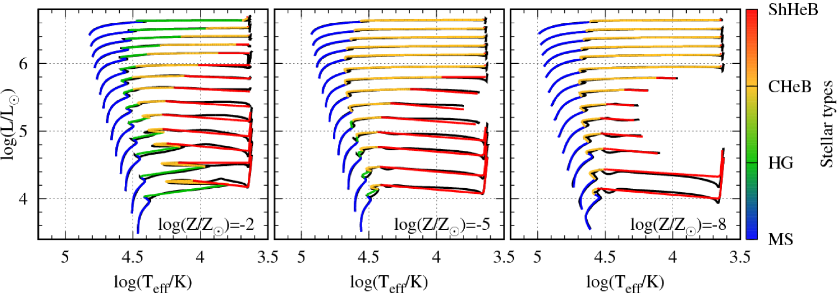
Figure 3: HR diagram for comparison between stellar models shown in Figure 1 (black curves), and fitting formulae calculated in the SSE code (colored curves). The color is coded according to stellar phases: MS, HG, CHeB, and ShHeB phases.

We follow the time evolution of stars with $M=8,10,13,16,20,25,32,40,50,65,80,100$, $125$, and $160M_{\odot}$ for $\log(Z/Z_{\odot})=-2,-5$ and $-8$. In Figure 3, we compare our fitting formulae with our stellar models shown in Figure 1. We can see that our fitting formulae are in a good agreement with our stellar models. For $\log(Z/Z_{\odot})=-8$, stars with $13\leq M/M_{\odot}<50$ end with BSG stars, and other stars become RSG stars at the ending time of their evolutions. Stars with $M/M_{\odot}<13$ have entered into their ShHeB phases by the time they become RSG stars. On the other hand, stars with $M/M_{\odot}\geq 50$ still remain CHeB stars when they become RSG stars. For $\log(Z/Z_{\odot})=-5$, the mass range of stars ending with BSG stars is decreased. The mass range is $20\leq M/M_{\odot}<50$. Moreover, stars with $M/M_{\odot}<25$ experience HG phases. Note that no stars experience HG phases for $\log(Z/Z_{\odot})=-8$. We compare our fitting formulae with our stellar models for $\log(Z/Z_{\odot})=-2$. All the stars enter into HG phases after MS phases. For $M/M_{\odot}<32$, stars experience blue loops after the HG phases. Finally, all the stars become RSG stars before they finish their lives. In our stellar models, the luminosity of the star with $M=65M_{\odot}$ is instantly decreased just before the star becomes a RSG star. We ignore this instant decrease of the luminosity to make the fitting formulae.

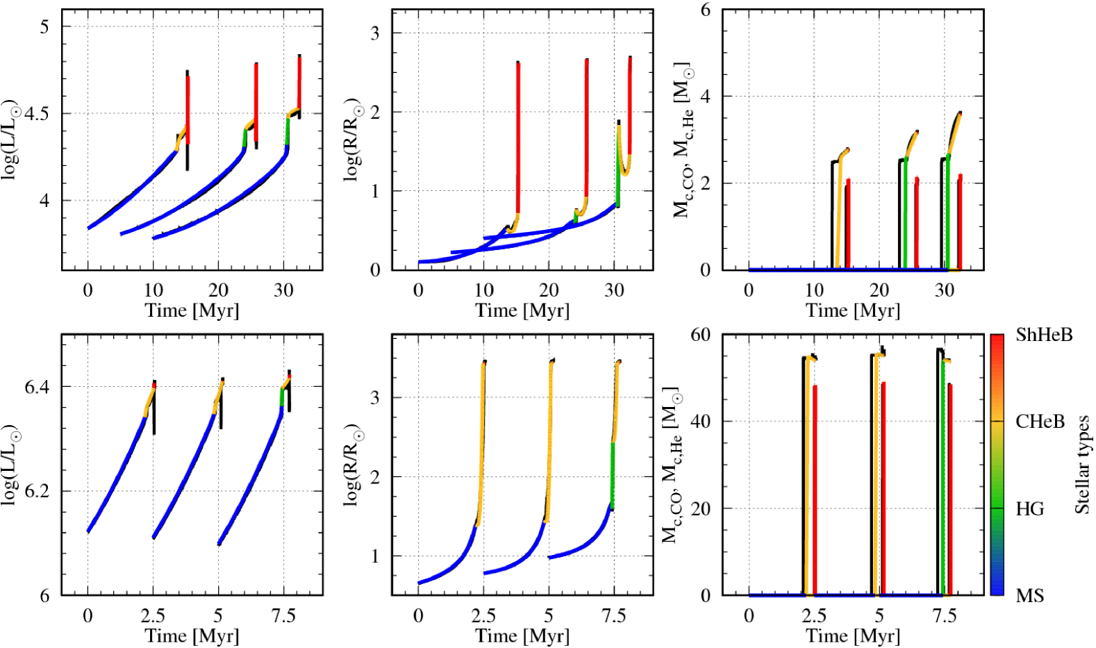
Figure 4: Time evolutions of luminosity, radius, He core mass, and CO core mass of stars with $M=10M_{\odot}$ (the top panels) and $M=100M_{\odot}$ (the bottom panels). In the rightmost panels, both of He and CO core masses are drawn, and the He core masses correspond to the larger curves. Each panel indicates these evolutions for $\log(Z/Z_{\odot})=-8,-5,-2$. The times are shifted by $5$ Myr and $10$ Myr for $M=10M_{\odot}$ with $\log(Z/Z_{\odot})=-5$ and $-2$, respectively, and by $2.5$ Myr and $5$ Myr for $M=100M_{\odot}$ with $\log(Z/Z_{\odot})=-5$ and $-2$, respectively. Black solid curves indicate our simulation data, and colored solid curves indicate our fitting formulae. The color codes are the same as Figure 3.

Figure 4 shows the time evolution of stars with $M=10$ and $100M_{\odot}$ for $\log(Z/Z_{\odot})=-2,-5$, and $-8$, and compare our fitting formulae (colored curves) with our simulation results (black curves). The leftmost panels draw the luminosity evolutions. We can see our fitting formulae capture features of luminosity evolutions except for instant decrease during the CHeB or ShHeB phases in our simulation data. The instant decrease occurs at the ending time of the BSG phases (at temperature of $\log(T_{\rm eff}/\mbox{K})\sim 10^{3.65}$ K) in our simulation data, as seen in Figures 1 and 3. Our fitting formulae deviate from our simulation data at the instant decreases, since we ignore the instant decreases for fitting formulae. At the ending time, our fitting formulae deviate from our simulation data by $\Delta\log L\lesssim 0.1$. The middle panels of Figure 4 compare the radius evolutions of our fitting formulae with those of our simulation data. These evolutions appear in a good agreement with each other for all the cases. The rightmost panels of Figure 4 indicate the time evolution of He and CO core masses. He cores in our fitting formulae grow later than those in our simulation data. This is because we set He core masses to be zero before the HG phases. CO cores in our fitting formulae also increase later than those in our simulation data. We assume that the CO core mass is zero before the ShHeB phases. We quantitatively investigate these deviations and their effects later. Note that we do not see clear metallicity dependence of the He core mass at the end of the main-sequence. This is partly because the overshoot effect erases metallicity dependence of He core mass (Limongi & Chieffi, 2018). Metallicity dependence of the He core mass is also discussed in Tornambe & Chieffi (1986).

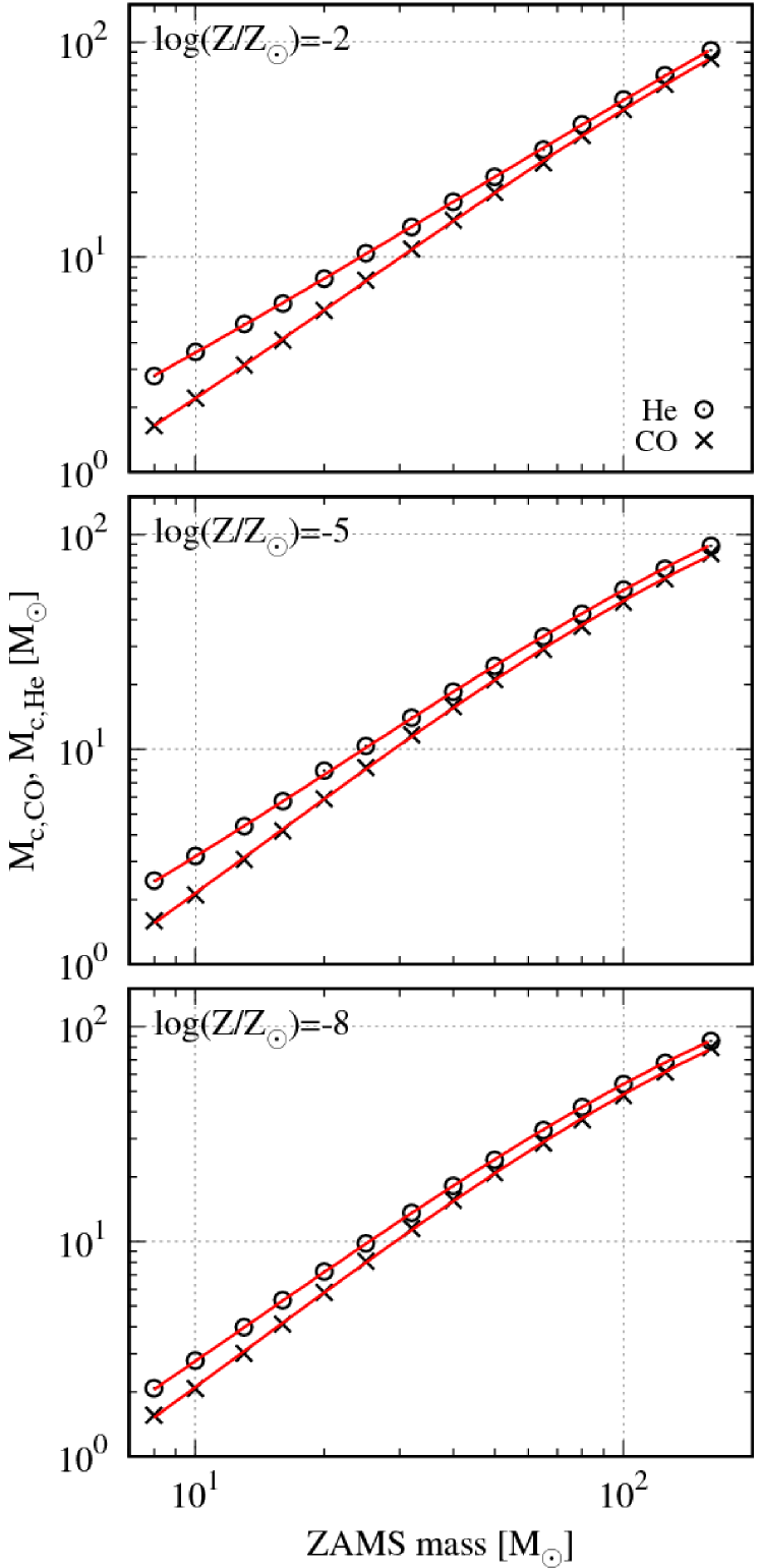
Figure 5: He (open circles) and CO (crosses) core masses at the ending times of the stellar evolutions as a function of ZAMS masses. Black points indicate our simulation data and red points indicate our fitting formulae. Note that the He and CO core masses in our fitting formulae correspond to $M_{\rm c,ShHeB}$ (Eq. (49)) and $M_{\rm c,CO}$ (Eq. (50)), respectively.

In Figure 5, we compare He and CO core masses in our fitting formulae with those in our simulation data. These core masses are $M_{\rm c,ShHeB}$ and $M_{\rm c,CO}$, i.e. ones at the ending times of the evolutions (see Eqs. (49) and (50), respectively). They are important, since they determine the remnant masses directly (see Eqs.(76), (79), and (83)). Our fitting formulae quite agree with our simulation data over $8\leq M/M_{\odot}\leq 160$. We will quantitatively discuss about this in more detail below.

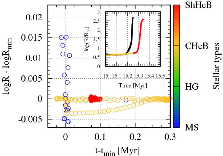
Figure 6: Deviations of radii between our fitting formulae and simulation data for $M=10M_{\odot}$ with $\log(Z/Z_{\odot})=-8$. The deviations are defined in the main text. The inset figure zooms in on the radius evolution of the ShHeB phase. The color codes are the same as Figure 3.

In order to evaluate deviations between our fitting formulae and simulation data, we define a distance between points of our fitting formulae and simulation data on time evolution diagrams like Figure 4 as

$$\Delta l=\min_{j}\left|\log\left(\frac{Qt}{Q_{j}t_{j}}\right)\right|,$$ (118)

where $Q$ ($Q_{j}$) indicates luminosity, radius, He core mass, or CO core mass of our fitting formulae (our simulation data) at time $t$ ($t_{j}$). This distance is helpful to quantify not only deviations of $Q$ between our fitting formulae and simulation data, but also deviations of stellar evolutionary times between them. If we rescale stellar evolutionary times of our fitting formulae so that their evolutionary times match corresponding stellar evolutionary times of our stellar evolution model, we should overlook the deviations of stellar evolutionary times. If we define the deviations such that $(Q-Q_{j})/Q_{j}$ at time $t$, the deviations should be overestimated for the following reason. Luminosity and radius rapidly grow at post-MS phases. Then, slight deviations of the beginning times of some phases (HG, CHeB, or ShHeB phases) raise large deviations of luminosities and radii between our fitting formulae and simulation data. This can be seen in the inset of Figure 6. The beginning time of the ShHeB phase deviates only by $\sim 0.1$ Myr, however $(Q-Q_{j})/Q_{j}\gtrsim 10^{2}$ at the beginning time.

Additionally, we define $Q_{\min}$ and $t_{\min}$ as those which are $Q_{j}$ and $t_{j}$, respectively, taking $\Delta l$ in Eq. (118). In other words, we can express $Q_{\min}$ and $t_{\min}$ as

$$\Delta l=\left|\log\left(\frac{Qt}{Q_{\min}t_{\min}}\right)\right|.$$ (119)

In Figure 6, we show the evolution of $(\log R-\log R_{\min},t-t_{\min})$ for the radius evolution seen in the inset. We can see that the radii themselves deviates by $\sim 3$ % in the MS phase, while the time deviates by at most $0.3$ Myr in the post-MS phases in the radius evolution.

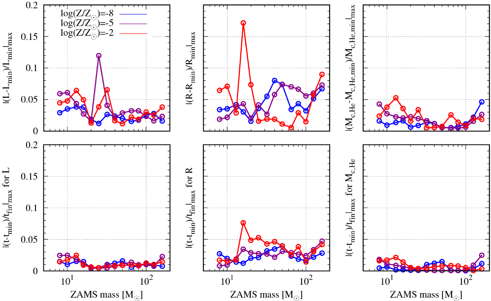
Figure 7: Maximum values of $(Q-Q_{\min})/Q_{\min}$ (top panels) and $(t-t_{\min})/t_{\min}$ (bottom panels) over the evolution of each star as a function of ZAMS mass.

Figure 7 shows the maximum values of $(Q-Q_{\min})/Q_{\min}$ and $(t-t_{\min})/t_{\min}$ over the evolution of each star. Except for the radii of $M=16M_{\odot}$ with $\log(Z/Z_{\odot})=-2$, the deviations are less than $\sim 10$ %. Even for $M=16M_{\odot}$ with $\log(Z/Z_{\odot})=-2$, the maximum deviation of its radius is $\sim 15$ %. It achieves this deviation at the ending time of the HG phase.

The maximum value of $(Q-Q_{\min})/Q_{\min}$ do not fully quantify deviations between our simulation data and fitting formulae. For example, the luminosity at the ending time in our fitting formula is less than that in our simulation data by $\Delta\log L\sim 0.05$ (or by $\sim 12$ %) for the case of $M=10M_{\odot}$ with $\log(Z/Z_{\odot})=-8$ (see the top left panel of Figure 4). On the other hand, $\left|(L-L_{\min})/L_{\min}\right|_{\max}\sim 3$ % as seen in Figure 7. This can be explained by the following reason. When we choose $L_{\min}$ for the luminosity at the ending time using Eq. (118), $L_{\min}$ is not the luminosity at the ending time in our simulation data, but the luminosity closest to luminosity at the ending time in our fitting formulae.

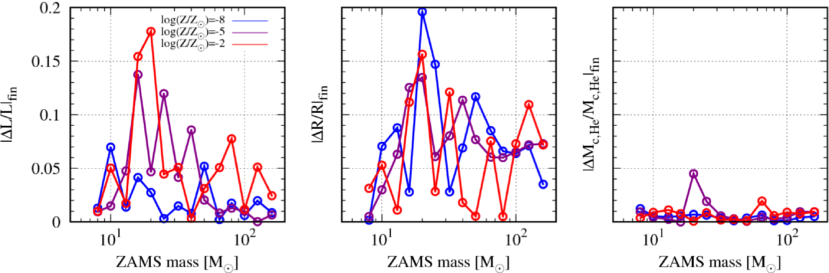
Figure 8: Deviations of quantities between our fitting formulae and simulation data at the ending times.

In order to solve this problem, we directly compare luminosities, radii, and He core masses in our fitting formula with those in our simulation data. Figure 8 shows these quantities at the ending time for our fitting formulae and simulation data. Then, we find these deviations are $\sim 20$ % at most, which is the radius at the ending time of $M=20M_{\odot}$ with $\log(Z/Z_{\odot})=-8$. These deviations in luminosities and radii tend to be large near $M/M_{\odot}\sim 20$ for the following reason. Stars with $M/M_{\odot}\lesssim 20$ reach to RSG stars, while stars with $M/M_{\odot}\gtrsim 20$ end with BSG stars. The luminosities and radii at the ending times strongly depend on stellar masses. Simple polynomials we use for our fitting formulae cannot follow such strong dependence. In contrast with the luminosities and radii at the ending time, the He and CO core masses at the ending time in our fitting formulae are different from in our simulation data by at most $5$ %.

Eventually, our fitting formulae deviate from our simulation data by at most $20$ %. We can say our fitting formulae have deviations small enough to be used for population synthesis calculations and star cluster simulations. These deviations are much smaller than uncertainties contained in population synthesis calculations and star cluster simulations, such as common envelope evolution.

4.2 Combination with a stellar wind model

In this section, we couple our fitting formulae with a stellar wind model described in section 3.6, and investigate stellar evolutions and their remnants.

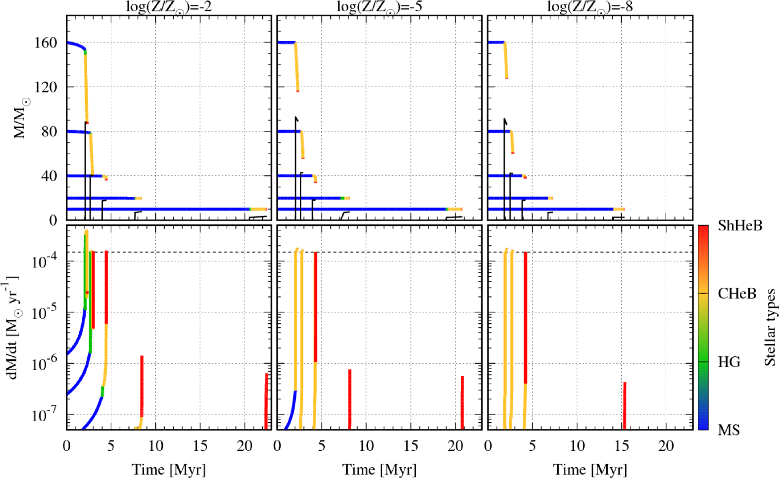
Figure 9: Time evolution of the total mass (top) and stellar wind mass loss (bottom) of stars with $10,20,40,80$, and $160M_{\odot}$ for $\log(Z/Z_{\odot})=-2,-5$, and $-8$. We can distinguish which curve is which stellar mass by the ending time of the evolution; the ending time is earlier as the stellar mass is larger. Black solid curves in the top panels indicate the time evolution of He core masses. Black dashed lines in the bottom panels indicate the mass loss of LBV stars $\dot{M}_{\rm LBV}=1.5\times 10^{-4}M_{\odot}\mbox{yr}^{-1}$. The color codes are the same as Figure 3.

Figure 9 shows time evolution of the total mass and stellar wind mass loss of stars with different masses and metallicities. Stars with $M/M_{\odot}\lesssim 40M_{\odot}$ receive little stellar wind mass loss for all the metallicities. This is owing to low metallicities. Stars with $M/M_{\odot}\gtrsim 80M_{\odot}$ significantly lose their masses in their CHeB phases. This mass loss is driven by LBV winds, $\dot{M}_{\rm LBV}$. This is true for all the metallicities, since the LBV mass loss does not depend on metallicity in our model. They lose their masses in their CHeB phases rather than in their ShHeB phases. This is mainly because the durations of their CHeB phases are longer than those of their ShHeB phases. The other reason is that a part of stars become naked He stars described below.

Stars with $\log(Z/Z_{\odot})=-2$ and $M/M_{\odot}\gtrsim 80M_{\odot}$ additionally receive the mass loss of luminous stars, $\dot{M}_{\rm NJ}$, from their MS phases to their CHeB phases. Note that their highest mass loss rates exceed the LBV mass loss rate $\dot{M}_{\rm LBV}=1.5\times 10^{-4}M_{\odot}\mbox{yr}^{-1}$. As a result of this, they become naked He stars. We can confirm this from the fact that their total masses are equal to their He core masses. When they are naked He stars, their mass loss rates are $\sim 6\times 10^{-6}M_{\odot}\mbox{yr}^{-1}$ for $M/M_{\odot}=80$, and $\sim 3\times 10^{-5}M_{\odot}\mbox{yr}^{-1}$ for $M/M_{\odot}=160$, dominated by the mass loss of WR stars. They might be observed as WR stars.

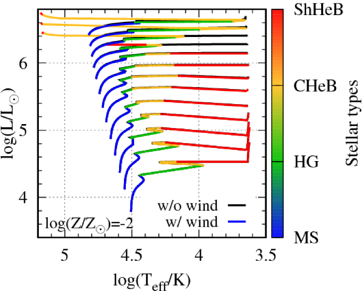
Figure 10: HR diagram of stars for $\log(Z/Z_{\odot})=-2$ with and without stellar wind mass loss (red and black curves, respectively). We do not show the evolution of a star with $M=8M_{\odot}$ at the ZAMS time, since its mass is decreased to $M/M_{\odot}<8$ due to the mass loss, and deviates from the scope of application of our fitting formulae. The color codes are the same as Figure 3.

We can follow stellar evolution to a naked He star by our fitting formulae, taking into account stellar wind mass loss by a post-processing way. Figure 10 shows the HR diagram of stars for $\log(Z/Z_{\odot})=-2$ with and without stellar wind mass loss. The evolutions of stars with $M/M_{\odot}\leq 65$ are similar regardless of the presence and absence of the mass loss. On the other hand, stars with $M/M_{\odot}\geq 80$ evolve blueward after the He ignition. This is because they become naked He stars for $M/M_{\odot}>80$, and nearly a naked He star for $M/M_{\odot}=80$ due to the mass loss. The mass boundary might be different from other evolution tracks due to difference of stellar evolution and wind models. However, the important point is that such a post-processing way to include stellar wind mass loss can represent the evolution to a naked He star.

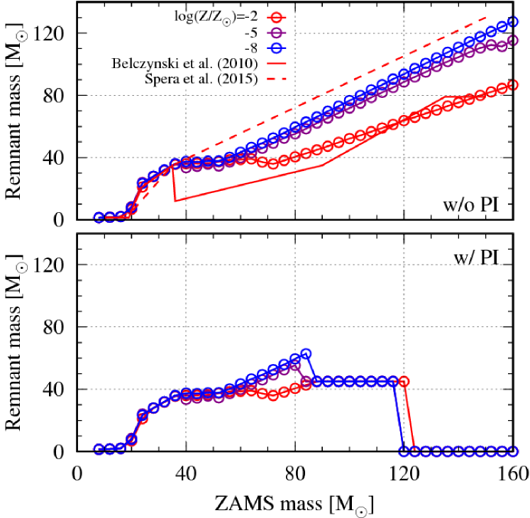
Figure 11: Relation between ZAMS star and their remnant masses for the w/o PI and w/ PI models (top and bottom, respectively). In the top panel, we add the relations of Belczynski’s and Spera’s models for $\log(Z/Z_{\odot})=-2$ (Belczynski et al., 2010; Spera et al., 2015, respectively). We read these data by eye from the literature.

Figure 11 shows the relation between ZAMS and remnant masses. We first focus on the w/o PI model. We compare our $\log(Z/Z_{\odot})=-2$ results with those of Belczynski et al. (2010). Stars with $M/M_{\odot}\lesssim 20$ leave NSs, which is consistent with them. BH masses left by stars with $20\lesssim M/M_{\odot}\lesssim 35$ are also in good agreement with them. BH masses left by stars with $M/M_{\odot}\gtrsim 60$ are larger than theirs by $10M_{\odot}$, since our He and CO core masses are more massive by $10M_{\odot}$. Nevertheless, the trend of the remnant masses in our fitting formulae is in good agreement with that in Belczynski et al. (2010). There is large discrepancy in BH masses in the range of stellar masses $35\lesssim M/M_{\odot}\lesssim 60$. These stars in our model receive LBV winds on shorter durations, since they have radii large enough to satisfy the LBV criterion (see Eq. (115)) on shorter durations. We find BH masses left by these stars are different among different evolution tracks. $40M_{\odot}$ stars leave BHs with $39M_{\odot}$ in our model, $15M_{\odot}$ in Belczynski et al. (2010), and $36M_{\odot}$ in SEVN (see fig. 14 in Spera et al., 2015). We conclude this discrepancy does not matter. The remnant masses for $\log(Z/Z_{\odot})=-5$, $-8$ are larger than for $\log(Z/Z_{\odot})=-2$, since stellar wind mass loss becomes weaker with metallicity decreasing. However, the remnant masses are similar between the cases of $\log(Z/Z_{\odot})=-5$ and $-8$. Stellar wind mass loss becomes ineffective for EMP stars, and does not sensitively depend on metallicity in this regime.

In $M/M_{\odot}\lesssim 80$, remnant masses in the w/ PI model are the same as in the w/o PI model. Otherwise, the former are smaller than the latter for all the metallicities due to PPI and PI SN effects. Remnant masses are $45M_{\odot}$ in $80\lesssim M/M_{\odot}\lesssim 120$ for all the metallicities. PPI work in this mass range. This is consistent with the relation between ZAMS and He core masses in Figure 5 which shows $45\lesssim M_{\rm c,He}/M_{\odot}\lesssim 65$ in $80\lesssim M/M_{\odot}\lesssim 120$. In $M/M_{\odot}\gtrsim 120$, remnant masses become zero, since these stars experience PI SNe. For $\log(Z/Z_{\odot})=-5$ and $-8$, stars with $M\sim 80M_{\odot}$ achieve the maximum remnant masses exceeding $45M_{\odot}$. This is because they do not undergo PPI nor PI SNe due to small He core masses, and leave hydrogen envelope owing to their low metallicities. On the other hand, the maximum remnant mass is $45M_{\odot}$ for $\log(Z/Z_{\odot})=-2$. Although stars with $M\sim 65M_{\odot}$ do not experience PPI nor PI SNe, they have no hydrogen envelope, and evolve to naked He stars at the ending time (see Figure 10). The lower mass limits of stars undergoing PPI and PI SNe in our fitting formulae are smaller than in the model of Belczynski et al. (2016b). This is because He core masses in our fitting formula are larger than in their model, as described above.

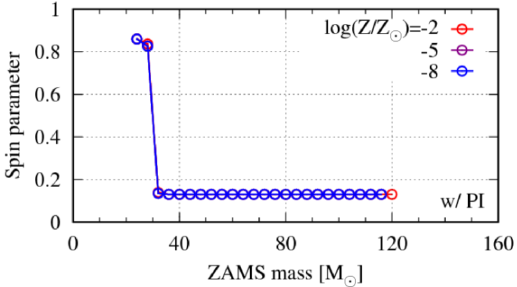
Figure 12: Relation between ZAMS star and their remnant spins for the w/ PI models.

Figure 12 shows remnant spins as a function of ZAMS mass for the w/ PI model. There is no data point in the mass range of $M/M_{\odot}\lesssim 20$ or $M/M_{\odot}\gtrsim 120$. This is because stars with $M/M_{\odot}\lesssim 20$ leave NSs, and those with $M/M_{\odot}\gtrsim 120$ leave no remnant due to PI SNe. BHs for the w/o PI model have the same spins when $M\lesssim 120M_{\odot}$. For the w/o PI, stars with $M\gtrsim 120M_{\odot}$ leave BHs with spins as low as stars with $M\sim 120M_{\odot}$ do.

5 Summary

We have devised the fitting formulae of EMP stars. Their metallicities are $\log(Z/Z_{\odot})=-2,-4,-5,-6$, and $-8$. The fitting formulae consider stars ending with BSG stars, and stars skipping HG phases and blue loops. In our fitting formulae, relatively light stars still remain BSG stars when they finish their CHeB phases. On the other hand, all the stars finish their BSG phases before they finish their CHeB phases in the Hurley’s models. This is not true especially for relatively light stars. Therefore, our modeling can be more realistic than the Hurley’s models. Our fitting formulae are in good agreement with our stellar models, which are consistent with Marigo’s model. Our fitting formulae can be used on the SSE, BSE, NBODY4, and NBODY6 codes for population synthesis calculations and star cluster simulations. We believe they should be useful to elucidate the origin of merging BH-BHs observed by gravitational wave observatories.

Appendix A Values for fitting formula

We show constants used in section 3.

Table 4: Constants for $\log(Z/Z_{\odot})=-2$.

$i$	0	1	2	3
${\cal T}_{{\rm HeI},i}$	+1.5839255604016800e+00	+7.9580658743321393e+01	+6.2605049204196496e+02	+4.9099525171608302e+03
${\cal T}_{{\rm CHeB},i}$	+1.9589322976358600e-01	+7.8483404642259504e+00	+4.5085546669210199e+00	+6.5327035939216103e+02
${\cal T}_{{\rm EBSG},i}$	+1.5491443477301301e+00	+1.0157506729497200e+02	+4.1045797870126700e+02	+6.5666106502774601e+03
${\cal T}_{{\rm Fin},i}$	+1.7829748399131200e+00	+8.7662108101897800e+01	+6.2980590516040002e+02	+5.6078890004744198e+03
${\cal L}_{{\rm ZAMS},i}$	-4.3387121453610497e-02	+4.7002611105589196e+00	-9.3228362169805801e-01	+5.8811945206418803e-02
${\cal L}_{{\rm EMS},i}$	-1.4163054579500700e-01	+6.2468925492728600e+00	-2.0517336248547200e+00	+2.7740223008074300e-01
${\cal L}_{{\rm HeI},i}$	+9.1569000891833996e-01	+4.5656469439486997e+00	-1.1002164667539900e+00	+9.3840594819720097e-02
${\cal L}_{{\rm ECHeB},i}$	+7.0984159927752299e-01	+5.2269835165592902e+00	-1.6253670199780199e+00	+2.1924040178420401e-01
${\cal L}_{{\rm EBSG},i}$	+1.6658494286226599e+00	+2.8135842651513001e+00	+1.0831049212944700e-01	-1.6438606141683301e-01
${\cal L}_{{\rm Fin,l},i}$	+7.1935042363085397e+00	-1.0757949651891300e+01	+1.2454591128743299e+01	-4.0650097608005700e+00
${\cal L}_{{\rm Fin,u},i}$	-1.0863563795046700e+00	+7.9383414627732600e+00	-2.9992532262892801e+00	+4.5364789567682801e-01
${\cal L}_{{\rm\alpha},i}$	-1.9408020240768799e-02	-8.9435341439184898e-02	+4.5147634586394197e-01	-1.5123156474279600e-01
${\cal L}_{{\rm\beta},i}$	-1.6671325813774601e-01	+4.3653653543205401e-01	-3.1149021748090500e-01	+6.7838974435627503e-02
${\cal L}_{{\rm\Delta},i}$	+6.7428636579205697e-02	+3.7982090032742701e-02	-5.7959714605753401e-02	+1.3089024896359399e-02
${\cal R}_{{\rm ZAMS},i}$	-3.6870298415699199e-01	+9.4401642726269397e-01	-2.1017534522620901e-01	+3.7277105006281598e-02
${\cal R}_{{\rm EMS},i}$	-1.4359719418587300e+00	+4.1335756478450900e+00	-2.4940809801056401e+00	+5.9090072146249595e-01
${\cal R}_{{\rm HeI},i}$	+4.9292595459292903e+00	-3.2253557317799100e+00	-7.3958869377935499e-01	+8.6851132826960398e-01
${\cal R}_{{\rm min},i}$	-3.0780806973814201e+00	+1.0260779580627400e+01	-8.2059416870071100e+00	+2.2289738933720402e+00
${\cal R}_{{\rm CHeB,EBSG},i}$	+6.1925984270592203e+00	-9.6076904024682896e+00	+5.6240568009227401e+00	-7.3097573061153098e-01
${\cal R}_{{\rm Fin},i}$	+0.0000000000000000e+00	+0.0000000000000000e+00	+0.0000000000000000e+00	+0.0000000000000000e+00
${\cal R}_{{\rm\alpha},i}$	-7.3471934070371600e-02	+2.5091437411072098e-01	-4.1162900537159798e-02	+8.9919312090114400e-03
${\cal R}_{{\rm\beta},i}$	-3.8906641158399602e-01	+1.1515583275404400e+00	-8.7408225106827897e-01	+2.7666584341436701e-01
${\cal R}_{{\rm\gamma},i}$	-1.0404715460267899e+00	+2.3176110463747399e+00	-1.7072675527739301e+00	+3.8380480274952700e-01
${\cal R}_{{\rm\Delta},i}$	-2.0879641699855300e-01	+3.7006200560629499e-01	-2.5730658470289097e-01	+4.8661473352442100e-02
${\cal R}_{{\rm RSG},0i}$	-8.7074249061240602e-02	-1.6922018399772801e-01
${\cal R}_{{\rm RSG},1i}$	+6.1896196949691396e-01	-5.7427447948830397e-03
${\cal H}_{{\rm HeI},i}$	-1.2316548227442199e+00	+1.8848911925803100e+00	-2.4609484339633700e-01	+2.2463422369182098e-02
${\cal H}_{{\rm ECHeB},i}$	-3.8303715910210101e-01	+7.0150741599662503e-01	+2.9607706988601801e-01	-5.9315517041934301e-02
${\cal C}_{{\rm CO},i}$	-7.3806577478145996e-01	+7.0263944811078005e-01	+5.0208830062187804e-01	-1.2376219079451400e-01

Table 5: Constants for $\log(Z/Z_{\odot})=-4$.

$i$	0	1	2	3
${\cal T}_{{\rm HeI},i}$	+1.5517508063147400e+00	+7.8762231265283901e+01	+6.6306742996156697e+02	+3.9780303119567002e+03
${\cal T}_{{\rm CHeB},i}$	+2.5995643378195399e-01	+1.3758291938603699e+00	+1.1749452241249701e+02	+7.3578237381483504e+01
${\cal T}_{{\rm EBSG},i}$	+1.5746855412155101e+00	+9.3014443586965996e+01	+5.9278989148185997e+02	+4.8922266924294800e+03
${\cal T}_{{\rm Fin},i}$	+1.8136363987309900e+00	+8.0465190932245406e+01	+7.7654726489562199e+02	+4.1226848652793597e+03
${\cal L}_{{\rm ZAMS},i}$	+7.0523683128112099e-03	+4.6392179589624503e+00	-9.0127242744985803e-01	+5.3238721546632901e-02
${\cal L}_{{\rm EMS},i}$	-9.5090922675450204e-02	+6.1861769329705298e+00	-2.0227268480957301e+00	+2.7233787294898498e-01
${\cal L}_{{\rm HeI},i}$	+5.5593067547365704e-01	+5.2576512230847499e+00	-1.5733536006708599e+00	+1.9982532305519199e-01
${\cal L}_{{\rm ECHeB},i}$	+1.0036121148808901e+00	+4.4477153532156501e+00	-1.0517047979711500e+00	+9.0669105159825694e-02
${\cal L}_{{\rm EBSG},i}$	+1.9138600333723099e+00	+2.0401605565817502e+00	+6.8545215127409798e-01	-2.9136581751254698e-01
${\cal L}_{{\rm Fin,l},i}$	+1.3665205743983201e+01	-2.8581615325979701e+01	+2.8565817023847401e+01	-8.8588379270868707e+00
${\cal L}_{{\rm Fin,u},i}$	-1.5295137595677000e+01	+3.1558544210358502e+01	-1.5855688265929601e+01	+2.7497620458708600e+00
${\cal L}_{{\rm\alpha},i}$	+7.7337632457581199e-02	-2.4681139438928901e-01	+5.3387040906391603e-01	-1.6557459200983801e-01
${\cal L}_{{\rm\beta},i}$	-4.3175574474877097e-02	+1.7703088876154599e-01	-1.3612814349929700e-01	+3.0317560049377499e-02
${\cal L}_{{\rm\Delta},i}$	-2.6732530743815101e-02	+2.2559320802858901e-01	-1.7984675493080099e-01	+3.8317535205556301e-02
${\cal R}_{{\rm ZAMS},i}$	-4.3620639472716299e-01	+8.4978687662735197e-01	-1.5993111424465600e-01	+2.7669651740859301e-02
${\cal R}_{{\rm EMS},i}$	-1.0109813992939201e+00	+2.8983622792063399e+00	-1.6345733256974599e+00	+4.0423625972161897e-01
${\cal R}_{{\rm HeI},i}$	+1.7618554313938800e-01	+2.0515198024096599e+00	-1.8411912436347599e+00	+6.0716387191588606e-01
${\cal R}_{{\rm min},i}$	-1.1462751987327799e+00	+4.0914478967912702e+00	-2.8790729602077900e+00	+7.8151962602801806e-01
${\cal R}_{{\rm CHeB,EBSG},i}$	+1.6237359045461699e+00	+5.6527800027967900e-01	-3.1779617931783601e+00	+2.0224444898627301e+00
${\cal R}_{{\rm Fin},i}$	+0.0000000000000000e+00	+0.0000000000000000e+00	+0.0000000000000000e+00	+0.0000000000000000e+00
${\cal R}_{{\rm\alpha},i}$	-3.0660053188372399e-01	+7.3518486490284396e-01	-3.7303325190354403e-01	+8.0660868408699404e-02
${\cal R}_{{\rm\beta},i}$	-1.1764079419992901e+00	+2.8256595551415500e+00	-2.0106042556923298e+00	+5.1511742066562305e-01
${\cal R}_{{\rm\gamma},i}$	+2.6666916897183601e-02	-5.6086994492167697e-02	-3.6193625945596802e-02	+1.4815537338410900e-02
${\cal R}_{{\rm\Delta},i}$	-1.7247613923205901e-01	+3.1501048172396900e-01	-2.3143156092273801e-01	+4.9808789329703798e-02
${\cal R}_{{\rm RSG},0i}$	+9.0940251890292804e-03	-2.3234236135069800e-01
${\cal R}_{{\rm RSG},1i}$	+5.9863657659087000e-01	+6.6527853775347704e-03
${\cal H}_{{\rm HeI},i}$	-1.0535947893773301e+00	+1.4170998603813501e+00	+1.2689928777198800e-01	-6.7494753025814203e-02
${\cal H}_{{\rm ECHeB},i}$	-3.9425104148142198e-01	+4.9002611835324500e-01	+5.7239586075853399e-01	-1.4093689615634999e-01
${\cal C}_{{\rm CO},i}$	-9.4823722226647700e-01	+9.7236386558568799e-01	+4.5283017654016999e-01	-1.3877489041026900e-01

Table 6: Constants for $\log(Z/Z_{\odot})=-5$.

$i$	0	1	2	3
${\cal T}_{{\rm HeI},i}$	+1.5608149013984800e+00	+7.3567160614509504e+01	+8.1835557597302898e+02	+2.1085273006198800e+03
${\cal T}_{{\rm CHeB},i}$	+2.5190328005023799e-01	+2.3937574545125400e+00	+6.8538719197550407e+01	+3.4090149355802299e+02
${\cal T}_{{\rm EBSG},i}$	+1.6461473568952700e+00	+8.5024735569825793e+01	+7.5746222377079403e+02	+3.0364037858196398e+03
${\cal T}_{{\rm Fin},i}$	+1.8149674275343299e+00	+7.6275812519002400e+01	+8.8345559090139704e+02	+2.5200002713951699e+03
${\cal L}_{{\rm ZAMS},i}$	+6.1565122879347303e-02	+4.5519847009521301e+00	-8.4909794442826203e-01	+4.2747189247281603e-02
${\cal L}_{{\rm EMS},i}$	-6.4010588830543502e-02	+6.1613002916478603e+00	-2.0261739188010601e+00	+2.7603556655566103e-01
${\cal L}_{{\rm HeI},i}$	+5.8122492862095898e-01	+5.1451646393334300e+00	-1.4989396222973901e+00	+1.8578769559084299e-01
${\cal L}_{{\rm ECHeB},i}$	+8.0634329880297295e-01	+4.7633074342534902e+00	-1.2175693546732000e+00	+1.1848267301948801e-01
${\cal L}_{{\rm EBSG},i}$	+1.4195127851226099e+00	+2.9963262421921000e+00	+9.7803246316281900e-02	-1.7525207469906401e-01
${\cal L}_{{\rm Fin,l},i}$	+1.4494199842344100e+01	-3.2273248268857600e+01	+3.3509908142265203e+01	-1.0945672335926499e+01
${\cal L}_{{\rm Fin,u},i}$	-2.9400093428201099e+00	+1.0683813612299200e+01	-4.2900521722222003e+00	+6.4299798091772997e-01
${\cal L}_{{\rm\alpha},i}$	+1.3507674415184301e-01	-3.1004292468722500e-01	+5.5482963687162401e-01	-1.6843671132819599e-01
${\cal L}_{{\rm\beta},i}$	-1.5512993576365000e-01	+3.7628702204329800e-01	-2.4439907829143701e-01	+4.8734830791039803e-02
${\cal L}_{{\rm\Delta},i}$	+6.8922515715162704e-03	+1.7942852148415400e-01	-1.6879676205781699e-01	+3.9630241617149800e-02
${\cal R}_{{\rm ZAMS},i}$	-4.2008197743730302e-01	+7.1601089423309805e-01	-8.7939534847640000e-02	+1.4674567587019200e-02
${\cal R}_{{\rm EMS},i}$	-9.2456828602432894e-01	+2.5389191763683798e+00	-1.3751410532902100e+00	+3.5045831707709002e-01
${\cal R}_{{\rm HeI},i}$	+3.9738040817917603e-01	+6.3392838342428004e-01	-4.8249880551521102e-01	+2.1465700473096400e-01
${\cal R}_{{\rm min},i}$	-6.4199204960415601e-01	+2.4849515765003098e+00	-1.5602241696515400e+00	+4.2012270812299601e-01
${\cal R}_{{\rm CHeB,EBSG},i}$	-7.8927435380812403e+00	+2.2851238614423899e+01	-2.0357967863018199e+01	+6.3389279382339296e+00
${\cal R}_{{\rm Fin},i}$	+2.4064199986630800e+02	-4.8538695379477701e+02	+3.2781854087263798e+02	-7.3251789698885403e+01
${\cal R}_{{\rm\alpha},i}$	-3.1420648674110302e-01	+7.3720759135681202e-01	-3.6998786143878298e-01	+7.8226901219150699e-02
${\cal R}_{{\rm\beta},i}$	-1.1538548374112800e+00	+2.7792891314058101e+00	-2.0035406799845701e+00	+5.2103603281852995e-01
${\cal R}_{{\rm\gamma},i}$	-9.9705770420161696e-03	+3.4151857848480502e-02	-1.2150727797915800e-01	+4.6426009888991697e-02
${\cal R}_{{\rm\Delta},i}$	-1.2237289829584599e-01	+1.7993028395168600e-01	-1.1080605018453900e-01	+1.9014426091513000e-02
${\cal R}_{{\rm RSG},0i}$	+5.6659069526797702e-02	-2.9401839565042698e-01
${\cal R}_{{\rm RSG},1i}$	+5.9229869792013501e-01	+1.5810282790358201e-02
${\cal H}_{{\rm HeI},i}$	-1.1011433924550000e+00	+1.5272663127372501e+00	+3.5517282030031301e-02	-4.3877721910985303e-02
${\cal H}_{{\rm ECHeB},i}$	-4.1085136748565099e-01	+4.4292411042459900e-01	+6.2270607618818596e-01	-1.5313454615055200e-01
${\cal C}_{{\rm CO},i}$	-9.2895961573096897e-01	+9.2331358192538004e-01	+4.7945677789672903e-01	-1.4307351573737101e-01

Table 7: Constants for $\log(Z/Z_{\odot})=-6$.

$i$	0	1	2	3
${\cal T}_{{\rm HeI},i}$	+1.5056408142507200e+00	+7.4994995850899201e+01	+8.3116022167663198e+02	+4.9040743535153001e+02
${\cal T}_{{\rm CHeB},i}$	+3.0667170921629699e-01	-2.2573597515177801e+00	+1.3262687600114401e+02	-4.3276720558498297e+01
${\cal T}_{{\rm EBSG},i}$	+1.6655342649798499e+00	+8.1652799673668696e+01	+8.2906385668603400e+02	+1.0852909614256901e+03
${\cal T}_{{\rm Fin},i}$	+1.8146885357058899e+00	+7.3040756282165205e+01	+9.6032575420450996e+02	+5.2267066025411305e+02
${\cal L}_{{\rm ZAMS},i}$	+8.6457066168576402e-02	+4.5267539598251902e+00	-8.3734602904147404e-01	+4.0772686211378001e-02
${\cal L}_{{\rm EMS},i}$	+7.0757975602064205e-02	+5.9547056937739100e+00	-1.9224648832190800e+00	+2.5857233194367901e-01
${\cal L}_{{\rm HeI},i}$	+4.4142301118520499e-01	+5.2539507603229101e+00	-1.4936383116696199e+00	+1.7333956725116800e-01
${\cal L}_{{\rm ECHeB},i}$	+5.5163281110466300e-01	+5.2726483070966701e+00	-1.5669073962725100e+00	+1.9653692229092701e-01
${\cal L}_{{\rm EBSG},i}$	+2.3653114492122501e-01	+5.3880332036350200e+00	-1.4180348147378099e+00	+1.3120380751216901e-01
${\cal L}_{{\rm Fin,l},i}$	-7.8189143203214698e+01	+2.3910265122146399e+02	-2.2922323244477499e+02	+7.3069269426524997e+01
${\cal L}_{{\rm Fin,u},i}$	+1.1685971748214700e-01	+5.9355760414335199e+00	-1.9145262506356799e+00	+2.5840425254712202e-01
${\cal L}_{{\rm\alpha},i}$	+7.1130274997986598e-01	-1.3554969336771401e+00	+1.1690764274913901e+00	-2.8733405856569799e-01
${\cal L}_{{\rm\beta},i}$	+8.7864061232266005e-02	-8.2310583604875406e-02	+2.2756522018622102e-02	-1.2808221435716401e-03
${\cal L}_{{\rm\Delta},i}$	+2.8862524329672300e-02	+1.2503925155034501e-01	-1.2931759799313100e-01	+3.0882782606178400e-02
${\cal R}_{{\rm ZAMS},i}$	-3.3237368336527201e-01	+4.6306428086272700e-01	+4.7820892172886598e-02	-9.6166327966181395e-03
${\cal R}_{{\rm EMS},i}$	-4.3397491671777300e-01	+1.3377594599674700e+00	-5.1421774804168696e-01	+1.5412807397524700e-01
${\cal R}_{{\rm HeI},i}$	+6.1860120021200900e-02	+4.0036628051026202e-01	+5.9419501733342803e-02	+4.0113003159862798e-02
${\cal R}_{{\rm min},i}$	-1.4216357295539300e-01	+7.8608012916942305e-01	-1.7661790431570801e-01	+8.7027362522545407e-02
${\cal R}_{{\rm CHeB,EBSG},i}$	-3.6832391211242701e+00	+1.1084061918623000e+01	-9.7324743496085198e+00	+3.1373519906345702e+00
${\cal R}_{{\rm Fin},i}$	+5.7804594901412303e+00	+4.2481043663905496e+00	-1.2931309320913600e+01	+5.6039641623863998e+00
${\cal R}_{{\rm\alpha},i}$	-3.8233593929888698e-01	+7.9002072854240402e-01	-3.4866555880093603e-01	+5.9835915587617299e-02
${\cal R}_{{\rm\beta},i}$	-7.1524193355817201e-01	+1.4559437723950699e+00	-8.4329698201959102e-01	+2.2410177619832200e-01
${\cal R}_{{\rm\gamma},i}$	+3.4301337795213799e-02	-1.2266252485565400e-01	+8.4527293107284907e-02	-2.7605337667557499e-02
${\cal R}_{{\rm\Delta},i}$	+5.0499661728335798e-01	-1.0261689627690800e+00	+6.2043697099474304e-01	-1.2325834401596100e-01
${\cal R}_{{\rm RSG},0i}$	-1.1360958843644700e-01	-1.4734021414496001e-01
${\cal R}_{{\rm RSG},1i}$	+6.2134621256327505e-01	-7.9113517758866905e-03
${\cal H}_{{\rm HeI},i}$	-1.1406439008233300e+00	+1.5754309620831299e+00	+1.5150861500077399e-02	-4.1230152708572498e-02
${\cal H}_{{\rm ECHeB},i}$	-5.2437528299791603e-01	+5.5932229149602297e-01	+5.7797948042505098e-01	-1.4589837221339999e-01
${\cal C}_{{\rm CO},i}$	-9.2137012965923404e-01	+8.8636637162070298e-01	+5.0592667147908199e-01	-1.4855704392558100e-01

Table 8: Constants for $\log(Z/Z_{\odot})=-8$.

$i$	0	1	2	3
${\cal T}_{{\rm HeI},i}$	+1.2305856460495901e+00	+1.0134578934187600e+02	+9.1468769124419097e+01	+1.8034769714629199e+03
${\cal T}_{{\rm CHeB},i}$	+2.4927377844451301e-01	+2.1430677547749402e+00	+8.5972144678894594e+01	-1.4028396903502400e+02
${\cal T}_{{\rm EBSG},i}$	+1.3730451469334499e+00	+1.0966949368516001e+02	+8.9197507907499698e+01	+2.0930245791822999e+03
${\cal T}_{{\rm Fin},i}$	+1.4810249724314000e+00	+1.0389495324882300e+02	+1.7328483361378301e+02	+1.7439035999222599e+03
${\cal L}_{{\rm ZAMS},i}$	-4.9125370974699000e-03	+4.7854346156440304e+00	-1.0218914733694000e+00	+8.0491993338893300e-02
${\cal L}_{{\rm EMS},i}$	+1.8683454969478600e-01	+5.7145070422311797e+00	-1.7657692128941300e+00	+2.2589703362508501e-01
${\cal L}_{{\rm HeI},i}$	+1.8683454969478600e-01	+5.7145070422311797e+00	-1.7657692128941300e+00	+2.2589703362508501e-01
${\cal L}_{{\rm ECHeB},i}$	+3.8790608169726498e-01	+5.4894852836696097e+00	-1.6450220435261300e+00	+2.0133843339575599e-01
${\cal L}_{{\rm EBSG},i}$	-7.8446922484086201e-01	+7.4136655401824401e+00	-2.6966654623657602e+00	+3.9086840832154501e-01
${\cal L}_{{\rm Fin,l},i}$	-5.2063766360667403e+00	+1.9423911281843100e+01	-9.4740006457763393e+00	+0.0000000000000000e+00
${\cal L}_{{\rm Fin,u},i}$	+2.2104250108866999e-01	+5.4053774623698096e+00	-1.3814930395748199e+00	+1.1265166679862200e-01
${\cal L}_{{\rm\alpha},i}$	+8.4548309048483195e-01	-1.2539875520793100e+00	+9.2320801185925605e-01	-2.0896705174094601e-01
${\cal L}_{{\rm\beta},i}$	-3.4823782284743299e-01	+6.6175971466374905e-01	-4.0197845268117299e-01	+7.9552888490381807e-02
${\cal L}_{{\rm\Delta},i}$	+1.6333532063424699e-01	-1.4798579565892800e-01	+4.7496374698078603e-02	-5.8983127069122503e-03
${\cal R}_{{\rm ZAMS},i}$	+4.6071669041284602e-01	-1.2482170192596500e+00	+1.1079694078714399e+00	-2.1778915454158501e-01
${\cal R}_{{\rm EMS},i}$	-8.7660234566099804e-01	+1.9194682681297499e+00	-7.3392245022216696e-01	+1.7274738264264999e-01
${\cal R}_{{\rm HeI},i}$	-8.7660234566099804e-01	+1.9194682681297499e+00	-7.3392245022216696e-01	+1.7274738264264999e-01
${\cal R}_{{\rm min},i}$	-8.7660234566099804e-01	+1.9194682681297499e+00	-7.3392245022216696e-01	+1.7274738264264999e-01
${\cal R}_{{\rm CHeB,EBSG},i}$	-1.8343478577029000e+01	+4.7783881233948101e+01	-4.0169462871126797e+01	+1.1460630304015901e+01
${\cal R}_{{\rm Fin},i}$	-7.8795250912748704e+00	+2.8961085855700901e+01	-2.8088036390052000e+01	+8.7716640685062703e+00
${\cal R}_{{\rm\alpha},i}$	-2.8687484575077300e+00	+5.4361579138011802e+00	-3.0890032437297399e+00	+6.0545880904935201e-01
${\cal R}_{{\rm\beta},i}$	-2.0581094227135899e+00	+3.8644269698339500e+00	-2.2704304648914801e+00	+5.0131612800208902e-01
${\cal R}_{{\rm\gamma},i}$	+6.2100077845129797e-01	-1.2611619209677001e+00	+7.8193448082669703e-01	-1.6755954354525801e-01
${\cal R}_{{\rm\Delta},i}$	+9.9983829393963303e-02	-4.4410431106289799e-01	+3.5725587872207698e-01	-8.6199515162683704e-02
${\cal R}_{{\rm RSG},0i}$	+1.9892249955808999e-01	-3.7299109886527798e-01
${\cal R}_{{\rm RSG},1i}$	+5.6071811071005395e-01	+3.2722143200640798e-02
${\cal H}_{{\rm HeI},i}$	-1.0733886890363700e+00	+1.4584928984676999e+00	+8.1519136854884905e-02	-5.3730041751472800e-02
${\cal H}_{{\rm ECHeB},i}$	-7.2712749189720804e-01	+8.3176655071820205e-01	+4.7853206104410101e-01	-1.3980539673247300e-01
${\cal C}_{{\rm CO},i}$	-9.5225083520154796e-01	+9.4357015904211505e-01	+4.7429337580493902e-01	-1.4351236491880501e-01

Appendix B Other metallicities

In this section, we present comparison between our fitting formulae and reference stellar models for $\log(Z/Z_{\odot})=-4$ and $-6$. Figures 13, 14, and 15 corresponds to Figure 3, 4, and 5, respectively. They match well each other.

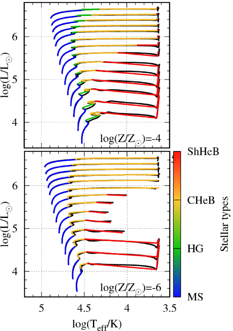
Figure 13: The same as Figure 3, except for $\log(Z/Z_{\odot})=-4$ and $-6$.

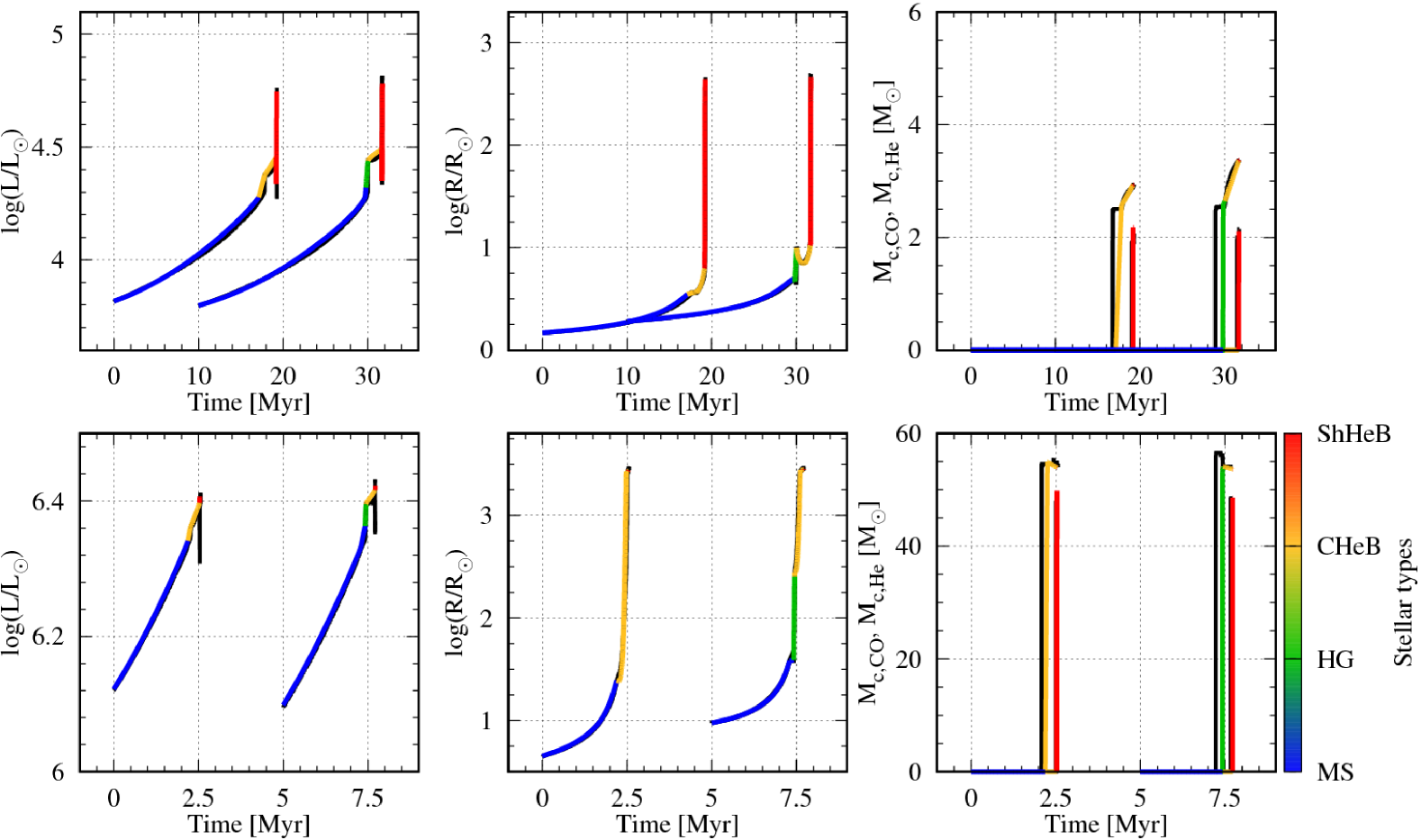
Figure 14: The same as Figure 14, except for $\log(Z/Z_{\odot})=-4$ and $-6$. The times are shifted by $10$ Myr for $M=10M_{\odot}$ with $\log(Z/Z_{\odot})=-4$, and by $5$ Myr for $M=100M_{\odot}$ with $\log(Z/Z_{\odot})=-2$.

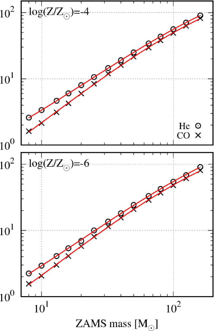
Figure 15: The same as Figure 5, except for $\log(Z/Z_{\odot})=-4$ and $-6$.

References

- Aarseth (2003) Aarseth S. J., 2003, Gravitational N-Body Simulations
- Abbott et al. (2016) Abbott B. P., et al., 2016, Physical Review Letters, 116, 061102
- Abbott et al. (2019) Abbott B. P., et al., 2019, Physical Review X, 9, 031040
- Abel et al. (2002) Abel T., Bryan G. L., Norman M. L., 2002, Science, 295, 93
- Asplund et al. (2009) Asplund M., Grevesse N., Sauval A. J., Scott P., 2009, ARA&A, 47, 481
- Bae et al. (2014) Bae Y.-B., Kim C., Lee H. M., 2014, MNRAS, 440, 2714
- Banerjee (2017) Banerjee S., 2017, MNRAS, 467, 524
- Banerjee et al. (2010) Banerjee S., Baumgardt H., Kroupa P., 2010, MNRAS, 402, 371
- Belczynski et al. (2002) Belczynski K., Kalogera V., Bulik T., 2002, ApJ, 572, 407
- Belczynski et al. (2010) Belczynski K., Bulik T., Fryer C. L., Ruiter A., Valsecchi F., Vink J. S., Hurley J. R., 2010, ApJ, 714, 1217
- Belczynski et al. (2014) Belczynski K., Buonanno A., Cantiello M., Fryer C. L., Holz D. E., Mand el I., Miller M. C., Walczak M., 2014, ApJ, 789, 120
- Belczynski et al. (2016a) Belczynski K., Holz D. E., Bulik T., O’Shaughnessy R., 2016a, Nature, 534, 512
- Belczynski et al. (2016b) Belczynski K., et al., 2016b, A&A, 594, A97
- Belczynski et al. (2017) Belczynski K., Ryu T., Perna R., Berti E., Tanaka T. L., Bulik T., 2017, MNRAS, 471, 4702
- Bethe & Brown (1998) Bethe H. A., Brown G. E., 1998, ApJ, 506, 780
- Blinnikov et al. (1996) Blinnikov S. I., Dunina-Barkovskaya N. V., Nadyozhin D. K., 1996, ApJS, 106, 171
- Böhm-Vitense (1958) Böhm-Vitense E., 1958, Z. Astrophys., 46, 108
- Bromm (2013) Bromm V., 2013, Reports on Progress in Physics, 76, 112901
- Bromm & Larson (2004) Bromm V., Larson R. B., 2004, ARA&A, 42, 79
- Bromm & Loeb (2003) Bromm V., Loeb A., 2003, Nature, 425, 812
- Brott et al. (2011) Brott I., et al., 2011, A&A, 530, A115
- Cassisi & Castellani (1993) Cassisi S., Castellani V., 1993, ApJS, 88, 509
- Cassisi et al. (2007) Cassisi S., Potekhin A. Y., Pietrinferni A., Catelan M., Salaris M., 2007, ApJ, 661, 1094
- Caughlan & Fowler (1988) Caughlan G. R., Fowler W. A., 1988, Atomic Data and Nuclear Data Tables, 40, 283
- Chiaki et al. (2016) Chiaki G., Yoshida N., Hirano S., 2016, MNRAS, 463, 2781
- Clark et al. (2011a) Clark P. C., Glover S. C. O., Smith R. J., Greif T. H., Klessen R. S., Bromm V., 2011a, Science, 331, 1040
- Clark et al. (2011b) Clark P. C., Glover S. C. O., Klessen R. S., Bromm V., 2011b, ApJ, 727, 110
- Cyburt et al. (2010) Cyburt R. H., et al., 2010, ApJS, 189, 240
- Dayal & Ferrara (2018) Dayal P., Ferrara A., 2018, Phys. Rep., 780, 1
- Di Carlo et al. (2019a) Di Carlo U. N., Mapelli M., Bouffanais Y., Giacobbo N., Bressan S., Spera M., Haardt F., 2019a, arXiv e-prints, p. arXiv:1911.01434
- Di Carlo et al. (2019b) Di Carlo U. N., Giacobbo N., Mapelli M., Pasquato M., Spera M., Wang L., Haardt F., 2019b, MNRAS, 487, 2947
- Dominik et al. (2012) Dominik M., Belczynski K., Fryer C., Holz D. E., Berti E., Bulik T., Mand el I., O’Shaughnessy R., 2012, ApJ, 759, 52
- Dominik et al. (2013) Dominik M., Belczynski K., Fryer C., Holz D. E., Berti E., Bulik T., Mand el I., O’Shaughnessy R., 2013, ApJ, 779, 72
- Drout et al. (2009) Drout M. R., Massey P., Meynet G., Tokarz S., Caldwell N., 2009, ApJ, 703, 441
- Ekström et al. (2008) Ekström S., Meynet G., Chiappini C., Hirschi R., Maeder A., 2008, A&A, 489, 685
- Eldridge & Stanway (2016) Eldridge J. J., Stanway E. R., 2016, MNRAS, 462, 3302
- Eldridge et al. (2017) Eldridge J. J., Stanway E. R., Xiao L., McClelland L. A. S., Taylor G., Ng M., Greis S. M. L., Bray J. C., 2017, Publ. Astron. Soc. Australia, 34, e058
- Eldridge et al. (2019) Eldridge J. J., Stanway E. R., Tang P. N., 2019, MNRAS, 482, 870
- Ferguson et al. (2005) Ferguson J. W., Alexander D. R., Allard F., Barman T., Bodnarik J. G., Hauschildt P. H., Heffner-Wong A., Tamanai A., 2005, ApJ, 623, 585
- Frebel & Norris (2015) Frebel A., Norris J. E., 2015, ARA&A, 53, 631
- Fujii et al. (2017) Fujii M. S., Tanikawa A., Makino J., 2017, PASJ, 69, 94
- Gerosa et al. (2018) Gerosa D., Berti E., O’Shaughnessy R., Belczynski K., Kesden M., Wysocki D., Gladysz W., 2018, Phys. Rev. D, 98, 084036
- Giacobbo & Mapelli (2018) Giacobbo N., Mapelli M., 2018, MNRAS, 480, 2011
- Giersz et al. (2013) Giersz M., Heggie D. C., Hurley J. R., Hypki A., 2013, MNRAS, 431, 2184
- Greif et al. (2011) Greif T. H., Springel V., White S. D. M., Glover S. C. O., Clark P. C., Smith R. J., Klessen R. S., Bromm V., 2011, ApJ, 737, 75
- Greif et al. (2012) Greif T. H., Bromm V., Clark P. C., Glover S. C. O., Smith R. J., Klessen R. S., Yoshida N., Springel V., 2012, MNRAS, 424, 399
- Hamann & Koesterke (1998) Hamann W. R., Koesterke L., 1998, A&A, 335, 1003
- Hartwig et al. (2016) Hartwig T., Volonteri M., Bromm V., Klessen R. S., Barausse E., Magg M., Stacy A., 2016, MNRAS, 460, L74
- Hirano et al. (2015) Hirano S., Hosokawa T., Yoshida N., Omukai K., Yorke H. W., 2015, MNRAS, 448, 568
- Hirschi (2007) Hirschi R., 2007, A&A, 461, 571
- Hong et al. (2018) Hong J., Vesperini E., Askar A., Giersz M., Szkudlarek M., Bulik T., 2018, MNRAS, 480, 5645
- Hosokawa et al. (2011) Hosokawa T., Omukai K., Yoshida N., Yorke H. W., 2011, Science, 334, 1250