Hamilton’s Dynamics in Complex Phase Space

Abstract

We present the basic formulation of Hamilton dynamics in complex phase space. We extend the Hamilton’s function by including the imaginary part and find out the corresponding Hamilton’s canonical equation of motion. Example of simple harmonic motion are considered and the corresponding trajectory are plotted on real and complex phase space.

Let $H(q,p,t)=U(q,p,t)+jV(q,p,t)$ be a complex Hamilton’s function H1 ; H2 ; H3 in complex phase space, where $q$ is the generalized coordinate and $p$ the conjugate generalized momentum defined on the phase space $(q,p)$. The total differentiation of the Hamiltonian $H(q,p,t)$ is given by

$$dH={\partial U\over\partial q}dq+j{\partial V\over\partial q}dq+{\partial U\over\partial p}dp+j{\partial V\over\partial p}dp+{\partial H\over\partial t}dt$$ (1)

The relation of Lagrangian function $L(q,\dot{q},t)$ with Hamilton’s function is defined by the following equation

$$H=p\dot{q}-L(q,\dot{q},t)=p\dot{q}-\big{[}W(q,\dot{q},t)+jZ(q,\dot{q},t)\big{]}$$ (2)

Taking total differentiation of equation (2), we obtain

$$dH=pd\dot{q}+\dot{q}dp-{\partial L\over\partial\dot{q}}dq-i{\partial L\over\partial q}dq-{\partial L\over\partial t}dt$$ (3)

Defining the generalized momentum conjugate to $q$ as

$$p={\partial L\over\partial\dot{q}}$$ (4)

and using

$${\partial L\over\partial q}dq={d\over dt}{\partial L\over\partial\dot{q}}dq=\dot{p}dq$$ (5)

we obtain

$$dH=\dot{q}dp-\dot{p}dq-\big{(}\partial L/\partial t\big{)}dt$$ (6)

Since, $q$ and $p$ are independent variables, the variations of $dq$, $dp$ and $dt$ are mutually independent. As a result their coefficients must be equal in Equation (1) and (6). Hence

$$\dot{q}={\partial U\over\partial p}+j{\partial V\over\partial p}$$ (7)

$$\dot{p}=-{\partial U\over\partial q}-j{\partial V\over\partial q}$$ (8)

and

$${\partial H\over\partial t}=-{\partial L\over\partial t}$$ (9)

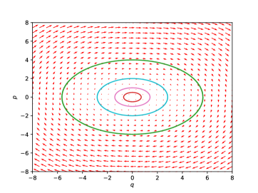
(a)

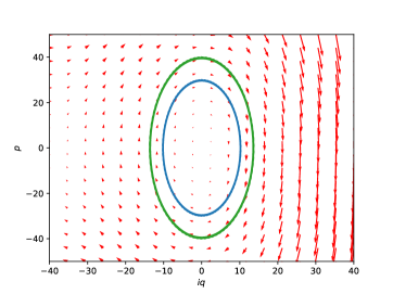
(b)

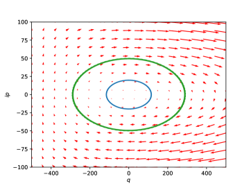
(c)

Figure 1: Trajectories of simple harmonic motion on phase space $(q,p)$, $(jq,p)$ and $(q,jp)$.

These first-order differential equations are called as Hamilton’s canonical equation of motion. By considering a complex Hamilton function of the form $H(q,p,t)=U(q,p,t)+jV(q,p,t)$, we obtained the Hamilton’s canonical equation of motion for the Hamilton’s function $H(q,p,t)$ defined on complex phase space. In order to understand the Hamilton dynamics in complex phase-space, we consider an example of simple harmonic motion defined by the following Hamilton’s function $H(q,p,t)$ with imaginary part equal to zero,

$$H(q,p,t)=U(q,p,t)+jV(q,p,t)={P^{2}\over 2m}+{k\over 2}q^{2}$$

From equation (7,8,9), we have

$$\dot{q} ={\partial H\over\partial p}={p\over m}\qquad\dot{p}=-{\partial H\over\partial q}=-kq$$

$${\partial H\over\partial t}=0$$

Figure (1(a)) shown the phase space trajectory of simple harmonic motion.
Consider an example of simple harmonic motion defined by the following complex Hamilton’s function $H(q,p,t)$ with non-zero imaginary part,

$$H(q,p,t)=U(q,p,t)+jV(q,p,t)={P^{2}\over 2m}+j{k\over 2}q^{2}$$

The corresponding equation of motion can be written as

$$\dot{q} ={\partial H\over\partial p}={p\over m}\qquad\dot{p}=-{\partial H\over\partial q}=-jkq$$

$${\partial H\over\partial t}=0$$

Figure (1(b),1(c)) shown the trajectory of simple harmonic motion on complex phase space.

Let $F(q,p)$ and $H(q,p)$, with $H(q,p)=U(q,p)+jV(q,p)$, be two functions on phase space. Then the Poisson bracket is given by

$$[F,H]=[F,U]+j[F,V]$$ (10)

In particular, $[q_{i},q_{i}+jp_{k}]=[q_{i},q_{i}]+j[q_{i},p_{k}]=j\delta_{ik}$ and $[q_{i},jp_{k}]=[q,0]+j[q,p]=j\delta_{ik}$. With the help of Hamilton’s equations (7,8,9), we have

$${dF\over dt}=[F,H]+{\partial F\over\partial t}=[F,U]+j[F,V]+{\partial F\over\partial t}$$

Consider a bivariate Hamilton function $H^{\prime}(q,p)$ associated to the univariate Hamilton function $H(z)$ via $H^{\prime}(x,y)=U(x,y)+jV(x,y)=H(z)|_{z=x+jy}$. The total differential is defined as P

$$dH^{\prime}={\partial H^{\prime}(q,p)\over\partial q}dq+{\partial H^{\prime}(q,p)\over\partial p}dp$$

Using $H^{\prime}(q,p)=U(q,p)+jV(q,p)$, we obtain

$$dH^{\prime}={\partial U(q,p)\over\partial q}dq+j{\partial V(q,p)\over\partial q}dq$$

$$+{\partial U(q,p)\over\partial p}dp+j{\partial U(q,p)\over\partial p}dp$$

Since, $z=q+jp$ and $z^{*}=q-jp$, we have

$$dz=dq+jdp$$

$$dz^{*}=dq-jdp$$

and

$$dq={1\over 2}(dz+dz^{*})$$

$$dp={1\over 2j}(dz-dz^{*})$$

The total differential $dH$ of a complex valued Hamilton function $H(z)$ can be expressed as

$$dH={\partial H(z)\over\partial z}dz+{\partial H(z)\over\partial z^{*}}dz^{*}$$ (11)

where the Wirtinger derivatives W are defined by

$${\partial\over\partial z}={1\over 2}\Big{[}{\partial\over\partial q}-j{\partial\over\partial p}\Big{]}$$ (12)

$${\partial\over\partial z^{*}}={1\over 2}\Big{[}{\partial\over\partial q}+j{\partial\over\partial p}\Big{]}$$ (13)

Using $H=p\dot{q}-L$, we have

$$dH=pd\dot{q}+\dot{q}dp-{\partial L\over\partial z^{1}}dz^{1}-{\partial L\over\partial z^{1*}}dz^{1*}$$ (14)

where

$$z^{1} =(q+j\dot{q})$$

$$z^{1*} =(q-j\dot{q})$$

$$dq ={1\over 2}(dz^{1}+dz^{1*})$$

$$d\dot{q} ={1\over 2j}(dz^{1}-dz^{1*})$$

Equation (14) becomes

$$dH=pd\dot{q}+\dot{q}dp-{1\over 2}\Big{(}{\partial\over\partial q}-j{\partial\over\partial\dot{q}}\Big{)}L\big{(}dq+jd\dot{q}\big{)}$$

$$-{1\over 2}\Big{(}{\partial\over\partial q}+j{\partial\over\partial\dot{q}}\Big{)}L\big{(}dq-jd\dot{q}\big{)}$$ (15)

Using equation (4) and (5), equation (15) can be rewritten as

$$dH=\dot{q}dp-\dot{p}dq$$ (16)

Using $dq=(dz+dz^{*})/2$, and $dp=(dz-dz^{*})/2j$, we have

$$dH ={\dot{q}\over 2j}(dz-dz^{*})-{\dot{p}\over 2}(dz+dz^{*})$$ (17)

or

$$dH=\Big{(}{\dot{q}\over 2j}-{\dot{p}\over 2}\Big{)}dz-\Big{(}{\dot{q}\over 2j}+{\dot{p}\over 2}\Big{)}dz^{*}$$ (18)

Comparing the coefficient of $dz$ and $dz^{*}$ in equation (18) with equation (11), we obtain

$$\dot{q}=j\Big{(}{\partial\over\partial z}-{\partial\over\partial z^{*}}\Big{)}H$$ (19)

$$\dot{p}=-\Big{(}{\partial\over\partial z}+{\partial\over\partial z^{*}}\Big{)}H$$ (20)

Equation (19-20) are Hamilton equation of motion in complex phase space. Substituting back the Wirtinger derivatives (equation (12,13)) in equation (19-20), we obtain Hamilton equation of motion in real phase space;

$$\dot{q}={\partial H\over\partial p}$$ (21)

$$\dot{p}=-{\partial H\over\partial q}$$ (22)

Equation (19-20) are basic Hamilton’s canonical equation of motion which can be used to understand the dynamics of particles in complex phase space.

References

(1) William Rowan Hamilton, On a General Method in Dynamics,
Philosophical Transactions of the Royal Society, 247-308, 1834.
(2) William Rowan Hamilton, Second Essay on a General Method in Dynamics,
Philosophical Transactions of the Royal Society, 95-144, 1835.
(3) T. L. Chow, Classical Mechanics, 2nd Edition, Taylor and Francis Group, 2013.
(4) P. Henrici, Applied and Computational Complex Analysis, Volume 1: Power Series Integration Conformal Mapping Location of Zero,
Wiley-Interscience, 704, 1988.
(5) W. Wirtinger, Zur formalen Theorie der Funktionen von mehr komplexen Veränderlichen,
Mathematische Annalen, Volume 97,357-375, 1927.