Deconvolution of isotopic pattern in 2D-FTICR Mass Spectrometry of peptides and proteins

Abstract

Mass Spectrometry (MS) is a largely used analytical technique in biology with applications such as the determination of molecule masses or the elucidation of structural data. Fourier Transform Ion Cyclotron Resonance MS is one implementation of the technique allowing high resolution and mass accuracy and based on trapping ions in circular orbits thanks to powerful Electromagnetic fields. This method has been extended to two-dimensional analysis, this gives signals containing a lot more information, for a reasonable amount of time and samples. However, the data provided by such experiments cannot be stored in a classical manner and require some tools and architecture to store and compress data so that they remain accessible and usable without necessitating too much computer memory. The developed python program permits to turn these huge raw data into exploitable FTICR MS HDF5 formatted datasets which can be relatively rapidly and efficiently deconvolved and analysed using a Primal-Dual Splitting algorithm.

Introduction

Fourier Transform Ion Cyclotron Resonance Mass Spectrometry (FTICR-MS) allows to accurately measure the mass over charge ratio ($m/z$) of molecular ions in the gas phase. It is based on a trapping of ions in cyclotronic circular orbits in vacuum, thanks to a powerful uniform magnetic field [Marshall et al., 1998]. Each of the ions, when excited by a resonant Radio Frequency electric field will generate a time-dependent current which can be measured. Fourier Transformation of this signal allows to get the corresponding orbital frequencies and a mass spectrum is obtained from a calibration based on the approximate basic equation:

$$f_{c}=\frac{zB_{o}}{m}$$ (1)

where $f_{c}$ is the cyclotronic resonance frequency, $B_{o}$ is the strength of the static magnetic field, $m$ and $z$ respectively the mass and the charge of the orbiting ion. This technique affords a high resolution and mass accuracy which eases the molecular interpretation of detected ions by drastically decreasing the ambiguity of the possible assignments [Vijlder et al., 2017].

Unambiguous assignments are particularly important when mass spectrometry is used for a bottom-up characterisation of proteins in a biological extract. In this approach, all proteins are first partially enzymatically hydrolysed to peptides, and the peptides from this mixture are analysed by tandem MS. The mass of each peptides is measured as well as the mass of its fragments after fragmentation inside the spectrometer. Due to the complexity of the sample, the classical approach consists in first separating by high-resolution Liquid Chromatography, and analysing each peptides sequentially [Aebersold and Mann, 2016].

We explore here an alternative route, where the sample is analysed by two-dimensional FTICR mass spectrometry (2D-FTICR-MS)[Floris et al., 2018]. This global approach which does not require sample fractionation was proposed long ago[Pfändler et al., 1987] and has known a recent renewal thanks to the increase in the computer capacities[van Agthoven et al., 2013, 2019]. After introduction of the sample mixture, the fragment ions are collected at the end of a three pulses sequence that includes the fragmentation delay. The sequence is built so that the intensity of the fragment ions show a periodic dependence to the cyclotronic frequency of the parent ion. By varying a delay in the sequence, this frequency is sampled, and a bi-dimensional Fourier transform of the data leads to a 2D mass spectrum, where a fragmentation event leads to a peak located at the parent $m/z$ along the vertical ($F1$) axis and at the fragment $m/z$ along the horizontal ($F2$) axis.

The shape of the signals in a FTICR-MS spectrum is dominated by two independent phenomena, and is demonstrated in figure 1. The presence of stable isotopes, in particular ¹³C present at about 1.1% relatively to ¹²C, produces typical 2D isotopic patterns, which are a generalisation of the isotopic patterns classically observed in Mass Spectrometry, and produced by the statistical distribution of the stable isotopes in the molecule. The shape of the pattern is easily computed from the molecular formula and the charge state of the considered ion. A second phenomena is the experimental peak lineshape, which is dominated by the experimental details such as the transient duration, and ion cloud stability, and can be considered as constant for all signals.

A general procedure was recently proposed to perform a pattern recognition of the classical isotopic pattern [Cherni et al., 2018], which efficiently extract the monoisotopic mass and the charge state. It is based on a dictionary approach. The goal of this study is to explore the possibility to extend this approach to the 2D case. It should be noted that most information which has to be extracted from the 2D experiment is the most possible accurae position of the monoisotopic signal,

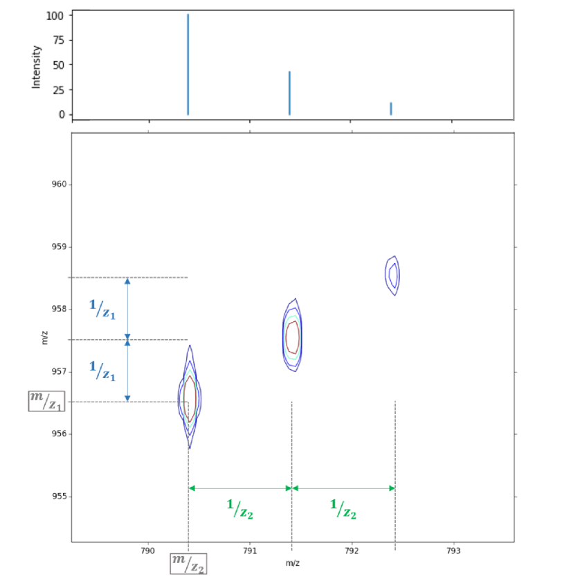
Figure 1: (bottom) Zoom on a typical isotopic pattern observed in 2D-FTICR-MS, here from the Yeast digest dataset. Peaks are separated along each dimensions by the inverse of the charge state $z_{1}$ and $z_{2}$, (here $z_{1}=z_{2}=1$) The monoisotopic peak is located at the lower left of the diagonal pattern. (top) the theoretical isotopic pattern computed with the averagine molecular model.

Materials and Methods

The raw 2D-FTICR experiment dataset was kindly sent to us by P.O’Connor from Warwick University. It is a yeast tryptic digest, on which a regular 2D experiment was performed on a 12 T Bruker Solarix FTICR mass spectrometer, using ESI ionisation and IRMPD fragmentation. 4096 $t_{1}$ increments were performed, for a total acquisition time of 54 minutes.

The encoding ($P1$) and excitation pulses ($P2$) were set to go from $460\,655\,$Hz to $263\,228\,$Hz, which correspond to a range of 400 to $700\,m/z$. The measurements along $F_{1}$ were made at a Nyquist frequency of $fn$ = $500\,000\,$Hz. The observed pulse ($P3$) was set to span the frequencies from $1\,250\,095\,$Hz to $61\,418\,$Hz, which correspond to a range of 147.4 to $3000\,m/z$. The acquisition spectral width was set to $1\,250\,095\,$Hz, corresponding to a low mass limit of $147.4\,m/z$.

Computer set-up

The analysis and computations were performed on a computer equipped with a processor Intel Xeon(®) CPU E3-1240 v5 at $3.50\,$GHz with 4 cores, 16GB of RAM and a graphical unit NVIDIA Quadro(®) K1200 with 4GB dedicated RAM.

Data Processing

The processing of the raw data obtained from the spectrometer were performed using the SPIKE library after being denoised with the SANE algorithm. SPIKE is a python library which is available on a public repository (http://www.bitbucket.org/delsuc/spike)[Chiron et al., 2016]. It allows to perform the complete processing of a raw 2D-FTICR-MS measurement, including the import, apodisation, peak-picking methods, HDF5 format compression. The deconvolution over compressed data is based on an algorithm designed for 1D deconvolution and extended to 2D, which is described in the Theory and Calculation section.

Experimental

Details on the Structure of the datasets

2D FTICR MS datasets are 2D maps, stored as matrices, and produced by a double Fourier transform step. Each entry is located at $(F_{1},F_{2})$ coordinates, expressed in $m/z$. While being 2D, this is not an image, and values are stored as double precision floating point values; visualisation is done by the computation of contour lines.

The 2D FTICR MS dataset is stored into a structured hierarchical HDF5 file. The data is a 2D matrix, and its size prohibits to load the data in memory, the HDF5 format allows to map the file content to memory, and this mode was chosen to access the data[The HDF Group, 1997, Dougherty et al., 2009]. The data matrix has to be accessed in a random manner in lines, columns, but also as 2D sub-domains. In a first level of structure, the matrix is stored using the CARRAY format proposed in HDF5. This format stores the data as sub-regions, stored as elementary piece of information, which allows an efficient random access, provided that all the required sub-regions can fit into memory. Extensive tests have been performed to optimize the size of these pieces.

However this organisation does not allow to easily produce global views of the data as it would be extremely slow. For this reason, in a second level of structure, a set of down-sampled matrices are computed from the original matrix, and store along side the original, using the possibilities of the HDF5 format. Several levels of down-sampling is used, allowing to have rapid and accurate accesses to the whole 2D spectrum, as well as large or local zooms. In the case of the dataset analysed here, the original matrix is 4k $\times$ 256k, and there are 4 down-sampled matrices, with sizes of 1k $\times$ 64k, 1k $\times$ 16k, 1k $\times$ 4k, and 1k $\times$ 1k, summing to more than a billion entries and a potential 9.3 Gigabyte of storage. The smaller matrix allows a fast access to the whole spectrum, while the intermediate sizes are used for views computed only on a part of the spectrum. A simple handling program allows to zoom in and out of the dataset, while always choosing the optimal matrix to use for the display.

As the dataset is composed of sharp peaks, located in an otherwise empty background, an optional further improvement has been implemented. A smaller file can be obtained by setting all values below a certain threshold to zero, and activating the internal lossless compression available in the HDF5 format. The threshold is typically chosen after an estimate of the background noise $\sigma$. In the case of the dataset analysed here, a threshold of $1\times\sigma$ produced a modest 17% compression without no visible modification of the spectrum, and a $3\times\sigma$ threshold gave a 82% compression, with some of the smallest features missing. With this set-up, dataset up to 8k x 512k are routinely handled on a simple laptop computer.

Core Code

The program development is done in python, a programming language conceived to be powerful but also easy to learn and to apply. The program relies on the following libraries NumPy for array processing[van der Walt et al., 2011], SciPy for scientific computing [Jones et al., 2001, Bressert [2012]], pytable for HDF5 files handling[Alted et al., 2002]. We use SPIKE [Chiron et al., 2016] a library developed for the analysis of NMR and MS data, for the general framework of the program.

Implementation on the whole 2D

To implement the deconvolution algorithm on the whole 2D dataset at the highest possible resolution, it is necessary to perform the calculations by chunks due to the huge size of data. To get these chunks, we use the memory mapping mode allowed by the pytable library, which avoid the loading of the complete dataset.

From this zone of interest to analyse, a list of the $N$ chunks coordinates of fixed sized in points is generated. In our set-up, chunks of $3072\times 256$ points were the most efficient as the processing is relatively fast and the size is large enough to accommodate full isotopic patterns (see Table 1).

For each zone, the deconvolution pattern is computed with a sliding approximation as presented below, using the averagine model [Senko et al., 1994] to estimate a typical molecular formula compatible with the local $m/z$, and a fast algorithm to estimate an isotopic pattern [Yergey, 1983, Kubinyi, 1991].

The deconvolution is then performed on each chunk on a slightly larger zone ($\pm 2m/z$ unit) than the chunk coordinates, in order to avoid any loss of information from patterns potentially cropped by the chunk border. At the end of the processing, the results is stored in a HDF5 file and memory is freed. The deconvolution results can then be loaded altogether to get a completely deconvolved spectra. The complete implementation of the program can be found at www.github.com/LauraDuciel/MSDeconv

Theory and Calculation

Problem formulation

Let us consider a MS spectrum, presented as a sequence of $(\{m_{p}^{\text{iso}}/z_{p},a_{p}\})_{1\leq p\leq N}$ where we denote by $m_{p}^{\text{iso}}\in(0,+\infty)$ the monoisotopic mass, $z_{p}\in\mathbb{N}^{*}$ design the charge state and $a_{p}\in(0,+\infty)$ is the abundance of the peptide $p\in\left\{1,\ldots,P\right\}$ in the chemical sample. We propose to model the acquired MS spectrum $y$ as the weighted sum of each individual isotopic pattern $y=\sum_{p=1}^{P}a_{p}\mathcal{\textit{D}}(m_{p}^{\text{iso}},z_{p})+n$ where $n$ models the acquisition noise and possible errors arising from the spectral analysis preprocessing step. The measurements are taken on a discrete grid of $(m/z)$ values with size $M$, so that the observation model finally reads:

$$\mathsf{\textbf{y}}=\sum_{p=1}^{P}a_{p}\mathsf{\textbf{d}}(m_{p}^{\text{iso}},z_{p})+\mathsf{\textbf{n}}$$ (2)

with $\mathsf{\textbf{y}}\in\mathbb{R}^{M}$, $\mathsf{\textbf{d}}(m_{p}^{\text{iso}},z_{p})\in[0,+\infty[^{M}$ and $\mathsf{\textbf{n}}\in\mathbb{R}^{M}$. The set of coefficients $(a_{p},m_{p}^{\text{iso}},z_{p})_{1\leq p\leq P}$ is not easily at hand because of the complicated and nonlinear function $\mathsf{\textbf{d}}(m,z)$ and the large value of $M$. The averagine model proposed by Senko et al. [1994] can be defined as a $\mathcal{A}:\,\mathbb{R}\rightarrow\mathbb{N}^{5}$ mapping between a mass value and the number of each atom present in the protein formula $\ce{C}_{N_{\ce{C}}}\ce{H}_{N_{\ce{H}}}\ce{O}_{N_{\ce{O}}}\ce{N}_{N_{\ce{N}}}\ce{S}_{N_{\ce{S}}}$. The result of averagine model on a given mass is a set of positions and their correspondent intensities presenting the abundances of present isotopes with their positions along the mass axis. We propose to use this model to build a dictionary-based approach under the assumption that we know approximately the range of mass and charge state for the $P$ proteins present in the sample. In general, the theoretical isotope distribution follows a multinomial distribution as it is presented in Kaur and O’Connor [2004] and can be represented with Gaussian or Lorentzian shapes. Consequently, the mass distribution function $\mathcal{\textit{D}}(m,z)$ is easy to evaluate from the molecular formula at a given $(m,z)$ values. In our work, we propose to generate $\mathcal{\textit{D}}(m,z)$ in the time domain with a Gaussian shape in order to have a sampled version $\mathsf{\textbf{d}}(m,z)$ on a defined mass grid. Then we use Fourier transform to map the spectrum domain. Here, we propose to normalize the result, so as to preserve the sum of squared amplitudes from $\mathcal{\textit{D}}(m,z)$ to $\mathsf{\textbf{d}}(m,z)$.

Isotopic deconvolution

For a given mass axis $[m_{\text{min}},m_{\text{max}}]$, and different charge states $z_{i}\in[z_{\text{min}},z_{\text{max}}]$, we propose to define a search grid with size $T:=MZ$ which defines $M$ possible values of isotopic masses and $Z$ possible values for the charges. From this grid, we build the dictionary $\mathsf{\textbf{D}}\in\mathbb{R}^{M\times T}$ noted as $\mathsf{\textbf{D}}=\left[\mathsf{\textbf{D}}_{1}\left|\ldots\right|\mathsf{\textbf{D}}_{\ell}\left|\ldots\right|\mathsf{\textbf{D}}_{Z}\right]$ where, for every $\ell\in\left\{1,\ldots,Z\right\}$, the sub-matrix $\mathsf{\textbf{D}}_{\ell}\in\mathbb{R}^{M\times M}$ maps for the dictionary associated to charge $\ell$. And each $i-$th column of $\mathsf{\textbf{D}}_{\ell}$ is considered as the isotopic pattern distribution $\mathsf{\textbf{d}}(m_{i},z_{i})$ depending on the mass $m_{i}$ and charge $z_{i}$ for every $m_{i}\in[m_{\min},m_{\max}]$ and $z_{i}\in[z_{\min},z_{\max}]$. Then, the problem is reformulated as:

$$\mathsf{\textbf{y}}=\mathsf{\textbf{D}}\mathsf{\textbf{x}}+\mathsf{\textbf{n}}^{\prime}$$ (3)

where x is a sparse vector with positive entries, for which the $P$ non-zeros coefficients allow to determine the isotopic mass and charge state of each protein, along with their abundance. Moreover, $\mathsf{\textbf{n}}^{\prime}=\mathsf{\textbf{n}}+\mathsf{\textbf{e}}$ models the acquisition noise and possible errors arising from the spectral analysis and discretization steps ($\mathsf{\textbf{n}}^{\prime}\rightarrow\mathsf{\textbf{n}}$ with high accuracy). With the ill-conditioning properties of dictionary D and the presence of noise, our problem is an inverse ill-posed problem. In addition, the large size of experimental MS spectrum requires efficient data processing algorithms, able to handle efficiently the large data sets involved. Based on the model in (3), the computation of D presents a challenge as large memory resources are needed to store this matrix. Therefore, we propose a new approximation based on Fourier transform. For similar mass values, isotopic patterns differ merely by a simple translation of peaks positions, and isotopic patterns can thus be considered locally stable, and the problem can locally be expressed as a strict convolution To avoid the storage of isotopic patterns for each $m/z$ value required by the dictionary-based approach, we decompose the mass axis into small windows onto which the isotopic pattern is assumed to be constant up to a circular shift. Let $L\leq M$ the chosen window width and $\overline{\mathsf{\textbf{d}}}_{s,\ell}$ the average isotopic pattern for a mass within the range $[(s-1)L+1,sL]$, and a fixed charge state $z_{\min}+(\ell-1)z_{\max}$. We propose to approximate each $\mathsf{\textbf{D}}_{\ell}$ by the following block diagonal (BDiag) matrix made of $M/L$ blocks assumed to be circulant (Circ) matrices with first line $\overline{\mathsf{\textbf{d}}}_{s,\ell}$, $s\in\left\{1,\ldots,M/L\right\}$:

$$\overline{\mathsf{\textbf{D}}}_{\ell}=\operatorname{BDiag}\left(\left[\text{Circ}\left(\overline{\mathsf{\textbf{d}}}_{s,\ell}\right)\right]_{1\leq s\leq M/L}\right).$$ (4)

As a consequence, the circulant approximation will be noted as $\overline{\mathsf{\textbf{D}}}=\left[\overline{\mathsf{\textbf{D}}}_{1}\left|\ldots\right|\overline{\mathsf{\textbf{D}}}_{\ell}\left|\ldots\right|\overline{\mathsf{\textbf{D}}}_{Z}\right]$ and for every charge value, the products $\overline{\mathsf{\textbf{D}}}_{\ell}$ and $\overline{\mathsf{\textbf{D}}}_{\ell}^{\top}$ with vectors can be easily computed using Fourier operations.

Implementation

A direct inversion of D to solve problem (3) and find an estimate of $\overline{\mathsf{\textbf{x}}}$ is not feasible because of the ill-conditioning character of D and the presence of noise. Therefore, we propose to employ a penalisation approach that defines the estimate $\widehat{\mathsf{\textbf{x}}}\in\mathbb{R}^{T}$ as a solution of the constrained minimization problem:

$$\underset{\begin{subarray}{c}{\mathsf{\textbf{x}}\in\mathbb{R}^{T}}\end{subarray}}{\mathrm{minimize}}\;\;\Phi(\mathsf{\textbf{x}})\quad\text{subject to}\quad\|\mathsf{\textbf{D}}\mathsf{\textbf{x}}-\mathsf{\textbf{y}}\|\leq\tau$$ (5)

where $\Phi:\mathbb{R}^{T}\mapsto(-\infty,+\infty]$ is the regularization function used to enforce positivity and sparsity on the solution, and $\tau>0$ is a parameter based on an estimate of experimental noise. The resolution of this problem requires to compute the proximal operator of function $\Phi$ at $x\in\mathbb{R}^{N}$, defined as the unique minimizer of $\Phi+\dfrac{1}{2}\|\cdot-x\|^{2}$ Moreau [1965], Bauschke and Combettes [2011]. This operator has been generalized for lower semicontinious and proper functions that are not necessarily convex in [Hiriart-Urruty and Lemaréchal, 1993, Sec.XV-4], as the multi-valued operator:

$$\operatorname{prox}_{\alpha\Phi}:\mathsf{\textbf{x}}\mapsto\underset{\mathsf{\textbf{y}}\in\mathbb{R}^{N}}{\operatorname{Argmin}}\quad\left(\frac{1}{2\alpha}\|\mathsf{\textbf{y}}-\mathsf{\textbf{x}}\|^{2}+\Phi(\mathsf{\textbf{y}})\right).$$ (6)

Using the variational formulation (5) we propose to use the proximal Primal-Dual Splitting algorithm from Chambolle and Pock [2011] which is an efficient algorithm for convex optimization and we choose to use the $\ell_{1}$ norm as a sparsity penality.

Algorithm 1 Primal-Dual Splitting Algorithm

$$\left\lfloor\begin{array}[]{l}\text{\bf Initialization}\\ \mathsf{\textbf{u}}^{(0)}\in\mathbb{R}^{M},\,\mathsf{\textbf{x}}^{(0)}\in\mathbb{R}^{T}\\ 0<\nu\kappa\|\mathsf{\textbf{D}}\|^{2}<1,\,\kappa>0\\ \rho\in(0,2)\\ \text{\bf Minimization}\\ \text{For}\;\;k=0,1,\ldots\\ \left\lfloor\begin{array}[]{l}\tilde{\mathsf{\textbf{x}}}^{(k)}=\operatorname{prox}_{\kappa\Phi}(\mathsf{\textbf{x}}^{(k-1)}-\kappa\mathsf{\textbf{D}}^{\top}(\mathsf{\textbf{u}}^{(k-1)}))\\ \mathsf{\textbf{v}}^{(k)}=\mathsf{\textbf{u}}^{(k-1)}+\nu\mathsf{\textbf{D}}(2\tilde{\mathsf{\textbf{x}}}^{(k)}-\mathsf{\textbf{x}}^{(k-1)})\\ \tilde{\mathsf{\textbf{u}}}^{(k)}=\mathsf{\textbf{v}}^{(k)}-\nu\text{proj}_{\|\cdot-\mathsf{\textbf{y}}\|\leq\tau}(\mathsf{\textbf{v}}^{(k)}/\nu)\\ \mathsf{\textbf{x}}^{(k)}=\mathsf{\textbf{x}}^{(k-1)}+\rho(\tilde{\mathsf{\textbf{x}}}^{(k)}-\mathsf{\textbf{x}}^{(k-1)})\\ \mathsf{\textbf{u}}^{(k)}=\mathsf{\textbf{u}}^{(k-1)}+\rho(\tilde{\mathsf{\textbf{u}}}^{(k)}-\mathsf{\textbf{u}}^{(k-1)})\\ \end{array}\right.\end{array}\right.$$

Here above, the projection operator $\text{proj}_{\|\cdot-\mathsf{\textbf{y}}\|\leq\tau}$ is defined, for every $(\mathsf{\textbf{y}},\mathsf{\textbf{v}})\in(\mathbb{R}^{N})^{2}$, as:

$$\text{proj}_{\|\cdot-\mathsf{\textbf{y}}\|\leq\tau}(\mathsf{\textbf{v}})=\mathsf{\textbf{v}}+(\mathsf{\textbf{v}}-\mathsf{\textbf{y}})\min\left(\frac{\tau}{\|\mathsf{\textbf{v}}-\mathsf{\textbf{y}}\|},1\right)-\mathsf{\textbf{y}}.$$ (7)

The convergence of the iterates $(\mathsf{\textbf{x}}^{(k)})_{k\in\mathbb{N}}$ to a solution of problem (5) is ensured, according to Chambolle and Pock [2011] and Condat [2013]. To estimate the mass and charge positions, Primal Dual algorithm can be easily used with the dictionary-based approach. Moreover, the 2D MS spectra can be efficiently analysed with a sample matricisation step. In this case, the convolution approximation approach can been used with little modifications where D is replaced by $\overline{\mathsf{\textbf{D}}}$ (4) and norm of $\overline{\mathsf{\textbf{D}}}$ is computed using power iteration.

Instrument response

In this process the physical model $\mathsf{\textbf{d}}(m,z)$ and its implementation $\overline{\mathsf{\textbf{D}}}$, comprehend the theoretical isotopic pattern and the instrument response function, which determines the width of the measured signal. Adding the instrument response to the model allows a deconvolution of the signal, and produces an enhancement of the linewidth along with the analysis of the $z$ value. Determination and optimization of the instrument function is required.

As an approximation, we assume that the instrument produces Gaussian lineshapes along both dimensions, and this is coded in the definition of $\overline{\mathsf{\textbf{D}}}$. We observed that the linewidth is more or less constant in frequency. Because of the inverse law between frequency and $m/z$ (Eq 1), this implies that the linewidth $\Delta m$ is proportional to $(m/z)^{2}$. Expressed in terms of resolution $R=m/\Delta m$, this means that $R$ is proportional to $\frac{1}{m/z}$ so that $Rm/z$ is a constant over the whole experiment, it could thus be estimated for some specific zones and applied globally. The optimal $Rm/z$ was estimated by varying the widthes and comparing the value of thr normalized $\chi^{2}$ at convergence, as shown on Figure 2. An optimum close but larger than $1.0$ indicates that the Gaussian approximation is correct but does not fully describes the instrument response. For the yeast data, it was estimated that $Rm/z=2.8\,10^{5}$ equivalent to $\Delta m/m^{2}=3.4\,10^{-6}$ on the vertical axis and $Rm/z=1.3\,10^{7}$ equivalent to $\Delta m/m^{2}=10^{-7}$ on the horizontal axis.

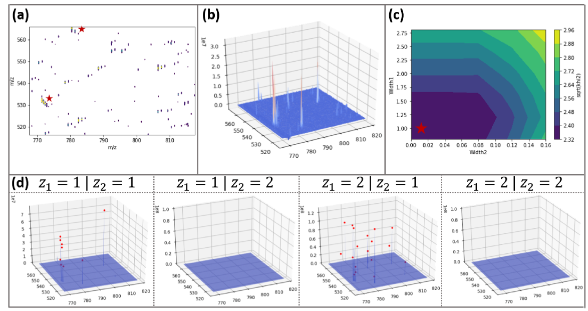
Figure 2: The deconvolution process, a) a zoomed region of the whole analysed dataset, the stars indicates signals from folded harmonics (see van Agthoven et al. [2019]); b) the same region as in a) shown in 3D; c) the value of $\sqrt{\chi^{2}}$ obtained when varying the width parameters along both axis, the star indicates the value used for the whole analysis; d) the result of the optimized deconvolution on the same region for the various $(z_{1},z_{2})$ pairs.

A peak picking and centroid centering was finally performed on the resulting reconstructed spectra, and the monoisotopic peak list listed. Here, 4300 peaks were retrieved after the deconvolution process and cleaning of impossible cases of $(z_{1},z_{2})$ pairs, to be compared with the 11078 peaks observed on the non-deconvoluted dataset. (Figure 3) This peak list can then directly be used for database search for the recognition of proteins such as Mascot or Prosight.

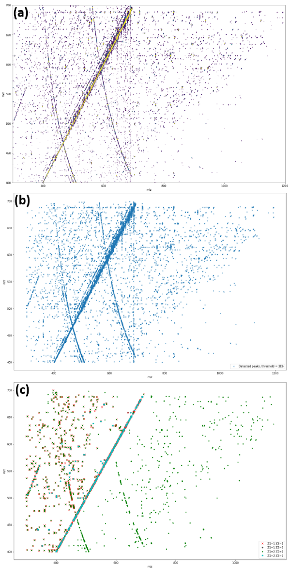
Figure 3: The result of the analysis of the complete 2D FTICR experiment using the optimised procedure. a) the original dataset; b) the result of the pattern analysis, with the superposition of the 4 $(z_{1},z_{2})$ analysed possibilities; c) the automatically detected peak from the dataset in b), with the superposition red: $(z_{1},z_{2})=(1,1)$, black: $(z_{1},z_{2})=(1,2)$, green: $(z_{1},z_{2})=(2,1)$, blue: $(z_{1},z_{2})=(2,2)$ showing the 4300 detected patterns. Note that because of physical reasons, only green peaks should be present below the diagonal.

Results

The application of this procedure on a yeast extract sample is presented in Figures 2 and 3 and in Table 1. Pattern recognition and monoisotopic analysis is successfully performed in a reasonable time considering the size and complexity of the dataset.

Computing times

The deconvolution of a 2D chunk is very dependent on the size of the chunks. Speed tests have been realized and show that the algorithm is more efficient on smaller chunks (Table 1). However, care has to be taken to insure chunks large enough to accommodate a complete pattern.

Chunk Sizes	Processing time observed for 1 chunk	Processing time expected for the whole experiment	Processing time observed for the whole experiment
$1024\times 256$	1 min 15 sec	18.3 h	12.6 h
$1536\times 256$	2 min 30 sec	24.5 h	14.8 h
$2048\times 256$	4 min 30 sec	33 h	15 h
$3072\times 256$	10 min 30 sec	51.5 h	20.4 h
$2048\times 512$	16 min 30 sec	70 h	not evaluated
$3072\times 384$	20 min	70 h	not evaluated

Table 1: Deconvolution processing times for various chunk sizes; observed processing time on the whole experiment include the $2m/z$ safety border

Taking into account these parameters, we estimated that the best chunk size choice would be $3072\times 256$, taking approximately $10\,$min $30\,$sec for the deconvolution of one chunk for $z\in[1,2]$ on the displayed zone. This selected chunk size offers good performances in terms of time and deconvolution efficiency. It was also observed that the deconvolution on highly compressed dataset was presenting artifacts and was clearly less efficient, probably due to bad convergence of the algorithm on zones containing too much zeros after the compression process.

The parameters should also be adapted to the computer set-up on which the calculations are performed. To get a result over the whole $4k\times 256k$ real points (representing more than a billion data points) with $3072\times 256$ chunks it took $20.4\,$hours on the tested computer described in the Materials and Methods part (Figure 3). It should finally be noted that this algorithm, decomposing the dataset in piecewise independent domain, can easily be parallelized on a larger system.

Discussion

Two-dimensional spectrometry such as 2D-FTICR-MS presents an exceptional analytical power, but introduces new challenges when compared to regular analytical measurements. Known in 2D Nuclear Magnetic Resonance (2D-NMR) spectroscopy for more than 30 years, problems such the size of datasets, the presence of non-local structured patterns, complex lineshapes have already been tackled and solved. Based on equivalent principles than 2D NMR, 2D FTICR-MS full development is only recent [van Agthoven et al., 2013] and these problems are not only present, but probably more stringent because of the size of the datasets.

The most important parameter in mass spectrometry is the determination of the exact position of spectral peaks, which determine the exact mass of the studied compound, in addition, the theoretical signal is always a $\delta$ function with no intrinsic width. For this reason, the decomposition of the instrument lineshape, as well as the non-local isotopic pattern to a single sharp peak is of importance. In addition, the size of the dataset enforces the use of complex data-storage, with hierarchical down-sampled representation and arrayed storage.

We show here that the methods developed to analyse classical FTMS spectra can be extended to the 2D case. The use of an optimized algorithm, based on a simplified dictionary allows to efficiently express the varying patterns to be recognized. In addition, the use of a HDF5 physical representation of the dataset insure an efficient data access, even with a limited memory, while allowing internally compressed files. The spectrum resulting from this analysis, was stored in the same manner, and presented very high compression ratio, thanks to the sparsity enforcing algorithm which generate dataset with many null values.

With this organisation, we were able to process in a compatible time a crowded, real life experiment, on a small desktop computer running with a limited memory and on only one processor. A parallel implementation of this algorithm was not performed but would be straightforward, and would insure high quality results in less than an hour when run on a larger computer or a small departmental cluster.

Conclusions

We have shown here that the method previously proposed for the analysis of 1D MS spectra and accurate determination of monoisotopic values by isotopic pattern matching [Cherni et al., 2018], can be extended to the 2D FTICR MS experiment. It was implemented and successfully applied on a real dataset. The code used in this work is open-source, and available at the following address: www.github.com/LauraDuciel/MSDeconv.

References

- Aebersold and Mann [2016] Ruedi Aebersold and Matthias Mann. Mass-spectrometric exploration of proteome structure and function. Nature News, 537(7620):347–355, 2016.
- Alted et al. [2002] Francesc Alted, Ivan Vilata, et al. PyTables: Hierarchical datasets in Python, 2002. URL http://www.pytables.org/.
- Bauschke and Combettes [2011] H.H. Bauschke and P.L. Combettes. Convex analysis and monotone operator theory in Hilbert spaces. CMS Books in Mathematics. Springer, New York, NY, 2011.
- Bressert [2012] Eli Bressert. SciPy and NumPy: An Overview for Developers. "O’Reilly Media, Inc.", 2012. ISBN 978-1-4493-6163-1.
- Chambolle and Pock [2011] A. Chambolle and T. Pock. A first-order primal-dual algorithm for convex problems with applications to imaging. J Math Imag Vis, 40(1):120–145, 2011.
- Cherni et al. [2018] Afef Cherni, Émilie Chouzenoux, and Marc-André Delsuc. Fast dictionary-based approach for mass spectrometry data analysis. IEEE International Conference on Acoustics, Speech and Signal Processing, pages 816–820, 2018.
- Chiron et al. [2016] Lionel Chiron, Marie-Aude Coutouly, Jean-Philippe Starck, Christian Rolando, and Marc-André Delsuc. SPIKE a Processing Software dedicated to Fourier Spectroscopies. arXiv:1608.06777 [physics], 2016. URL http://arxiv.org/abs/1608.06777. arXiv: 1608.06777.
- Condat [2013] L. Condat. A primal–dual splitting method for convex optimization involving Lipschitzian, proximable and linear composite terms. J Optim Theory Appli, 158(2):460–479, 2013. ISSN 1573-2878. doi: 10.1007/s10957-012-0245-9. URL https://doi.org/10.1007/s10957-012-0245-9.
- Dougherty et al. [2009] Matthew T. Dougherty, Michael J. Folk, Erez Zadok, Herbert J. Bernstein, Frances C. Bernstein, Kevin W. Eliceiri, Werner Benger, and Christoph Best. Unifying Biological Image Formats with HDF5. Commun ACM, 52(10):42–47, 2009. ISSN 0001-0782. doi: 10.1145/1562764.1562781. URL https://www.ncbi.nlm.nih.gov/pmc/articles/PMC3016045/.
- Floris et al. [2018] Federico Floris, Maria A van Agthoven, Lionel Chiron, Christopher A Wootton, Pui Yiu Yuko Lam, Mark P Barrow, Marc-André Delsuc, and Peter B O’Connor. Bottom-Up Two-Dimensional Electron-Capture Dissociation Mass Spectrometry of Calmodulin. J Am Soc Mass Spect, 29(1):207–210, 2018.
- Hiriart-Urruty and Lemaréchal [1993] J. B. Hiriart-Urruty and C. Lemaréchal. Convex analysis and minimization algorithms II: Advanced theory and bundle methods, volume 306 of Grundlehren der mathematischen Wissenschaften. Springer-Verlag, New York, 1993.
- Jones et al. [2001] Eric Jones, Travis Oliphant, Pearu Peterson, and Others. SciPy: Open source scientific tools for Python, 2001. URL http://www.scipy.org/. [Online; accessed 2016-04-20].
- Kaur and O’Connor [2004] Parminder Kaur and Peter B O’Connor. Use of statistical methods for estimation of total number of charges in a mass spectrometry experiment. Anal Chem, 76(10):2756–2762, 2004.
- Kubinyi [1991] H. Kubinyi. Calculation of isotope distributions in mass spectrometry. a trivial solution for a non-trivial problem. Anal Chim Acta, 247:107–119, 1991.
- Marshall et al. [1998] A G Marshall, C L Hendrickson, and G S Jackson. Fourier transform ion cyclotron resonance mass spectrometry: a primer. Mass Spectrom Rev, 17(1):1–35, 1998.
- Moreau [1965] J.-J. Moreau. Proximité et dualité dans un espace hilbertien. Bull Soc Chim France, 93:273–299, 1965.
- Pfändler et al. [1987] P Pfändler, G Bodenhausen, J Rapin, R Houriet, and T Gäumann. Two-dimensional fourier transform ion cyclotron resonance mass spectrometry. Chem Phys Let, 138(2):195–200, 1987.
- Senko et al. [1994] M.-W. Senko, J.-P Speir, and F.-W. McLafferty. Collisional activation of large multiply charged ions using Fourier transform mass spectrometry. Anal Chem, 66(18):2801–2808, 1994.
- The HDF Group [1997] The HDF Group. Hierarchical Data Format, version 5, 1997. http://www.hdfgroup.org/HDF5/.
- van Agthoven et al. [2013] Maria A van Agthoven, Marc-André Delsuc, Geoffrey Bodenhausen, and Christian Rolando. Towards analytically useful two-dimensional Fourier transform ion cyclotron resonance mass spectrometry. Anal Bioanal Chem, 405:51–61, 2013.
- van Agthoven et al. [2019] Maria A. van Agthoven, Yuko P. Y. Lam, Peter B. O’Connor, Christian Rolando, and Marc-André Delsuc. Two-dimensional mass spectrometry: new perspectives for tandem mass spectrometry. Eur Biophys J, 48(3):213–229, 2019. ISSN 1432-1017. doi: 10.1007/s00249-019-01348-5. URL https://doi.org/10.1007/s00249-019-01348-5.
- van der Walt et al. [2011] S. van der Walt, SC. Colbert, and G. Varoquaux. The numpy array: A structure for efficient numerical computation. Comput Sci Eng, 13:22–30, 2011.
- Vijlder et al. [2017] Thomas De Vijlder, Dirk Valkenborg, Filip Lemière, Edwin P. Romijn, Kris Laukens, and Filip Cuyckens. A tutorial in small molecule identification via electrospray ionization-mass spectrometry: The practical art of structural elucidation. Mass Spectrom Rev, 37(5):607–629, 2017. ISSN 0277-7037. doi: 10.1002/mas.21551. URL http://dx.doi.org/10.1002/mas.21551.
- Yergey [1983] J.-A. Yergey. A general approach to calculating isotopic distributions for mass spectrometry. Int J Mass Spec Ion Phys, 52(2-3):337–349, 1983.