On the Walks and Bipartite Double Coverings of Graphs with the same Main Eigenspace

Abstract

The main eigenvalues of a graph $G$ are those eigenvalues of the $(0,1)$-adjacency matrix $\mathbf{A}$ having a corresponding eigenvector not orthogonal to $\mathbf{j}=(1,\dots,1)$. The CDC of a graph $G$ is the direct product $G\times K_{2}$. The main eigenspace of $\mathbf{A}$ is generated by the principal main eigenvectors and is the same as the image of the walk matrix. A hierarchy of properties of pairs of graphs is established in view of their CDC’s, walk matrices, main eigenvalues, eigenvectors and eigenspaces. We determine by algorithm that there are 32 pairs of non-isomorphic graphs on at most 8 vertices which have the same CDC.

Keywords: Eigenvalues, walks, walk matrix, main eigenspace, canonical (bipartite) double covering, TF-isomorphism.

i   Introduction

A graph of order $n$ is a pair of sets $G=(\mathcalboondox V,\mathcalboondox E)$ where $\mathcalboondox V=\{1,\dots,n\}$ is called the set of vertices, and $\mathcalboondox E\subseteq\{\{u,v\}:u,v\in\mathcalboondox V\ \text{and}\ u\neq v\}$ is called the set of edges. (We consider graphs which are simple; that is, graphs which are undirected, without multiple edges or loops.) A $k$-walk in a graph $G$ is a $k$-tuple $(u_{0},u_{1},\dots,u_{k})\in\mathcalboondox V^{k+1}$ such that $\{u_{i-1},u_{i}\}\in\mathcalboondox E$ for all $1\leqslant i\leqslant k$.

The adjacency matrix of a graph $G$, denoted by $\mathbf{A}(G)$, or simply $\mathbf{A}$ where the context is clear, is the symmetric $n\times n$ matrix $\left(a_{ij}\right)$, where $a_{ij}=1$ if $\{i,j\}\in\mathcalboondox E$, and $a_{ij}=0$ otherwise. We use terminology for a graph $G$ and its adjacency matrix $\mathbf{A}$ interchangeably, since the graph $G$ is determined, up to relabelling of the vertices, by $\mathbf{A}$. For example, the eigenvalues and eigenvectors of a graph $G$ are respectively those of the matrix $\mathbf{A}$. The spectrum $\operatorname{spec}(G)$ of a graph $G$ is the multiset consisting of the $s$ distinct eigenvalues $\mu_{1},\dots,\mu_{s}$, each occurring $m(\mu_{i})$ times, $1\leqslant i\leqslant s$; where the multiplicity $m(\mu_{i})$ is the number of times that $\mu_{i}$ is repeated as a root of the characteristic polynomial $\det(\lambda\mathbf{I}-\mathbf{A})$. Since $\mathbf{A}$ is real-symmetric, we also have that $m(\mu_{i})$ is the dimension of the eigenspace $\mathop{\scalebox{1.2}{\text{E}}}{}_{G}(\mu_{i})$ associated with $\mu_{i}$, where $\mathop{\scalebox{1.2}{\text{E}}}{}_{G}(\mu_{i})=\{\mathbf{x}\in{\mathds{R}}^{n}:\mathbf{A}\mathbf{x}=\mu_{i}\mathbf{x}\}$, and $n=|\mathcalboondox V|$. Spectral decomposition of $\mathbf{A}$ yields

$$\mathbf{A}=\sum_{i=1}^{s}\mu_{i}\mathbf{P}_{i},$$ (1)

where $\mathbf{P}_{i}\colon{\mathds{R}}\to\mathop{\scalebox{1.2}{\text{E}}}{}_{G}(\mu_{i})$ is the orthogonal projection onto the eigenspace for $\mu_{i}$, $1\leqslant i\leqslant s$.

The entry $a_{ij}^{(k)}$ of the matrix $\mathbf{A}^{k}$ is the number of walks of length $k$ starting from vertex $i$ to vertex $j$. If $\mathbf{j}$ denotes the all-ones $n\times 1$ column $(1,\dots,1)$, then the $i$th entry of $\mathbf{A}^{k}\mathbf{j}$ is the total number of walks of length $k$ starting from vertex $i$. The $n\times k$ matrix whose $k$ columns are $\mathbf{A}^{i-1}\mathbf{j}$ for $i=1,2,\dots,k$ is called the $k$-walk matrix of $G$, denoted by $\mathbf{W}_{G}(k)$:

$$\mathbf{W}_{G}(k)=\begin{pmatrix}|&|&|&&|\\ \mathbf{j}&\mathbf{A}\mathbf{j}&\mathbf{A}^{2}\mathbf{j}&\cdots&\mathbf{A}^{k-1}\mathbf{j}\\ |&|&|&&|\end{pmatrix}.$$

The eigenvalues $\mu_{1},\mu_{2},\dots,\mu_{p}$ of $G$ ($1\leqslant p\leqslant n$) having an associated eigenvector not orthogonal to $\mathbf{j}$ (i.e. $\langle\mathbf{x},\mathbf{j}\rangle\neq 0$) are said to be main. The remaining distinct eigenvalues $\mu_{p+1},\mu_{p+2},\dots,\mu_{s}$ ($s\leqslant n$) are non-main. Walks and main eigenvalues are closely related—it turns out that the number of walks of length $k$ in $G$ is given by

$$N_{k}=\sum_{i=1}^{p}\big{\|}\mathbf{P}_{i}\,\mathbf{j}\big{\|}^{2}\,{\mu_{i}}^{k}=c_{1}{\mu_{1}}^{k}+c_{2}{\mu_{2}}^{2}+\cdots+c_{p}{\mu_{p}}^{k},$$

where $\mu_{i}$, $i=1,\dots,p$ are the main eigenvalues of $G$, $\mathbf{P}_{i}$ is as in equation 1, and $c_{i}\mathrel{\vbox{\hbox{\scriptsize.}\hbox{\scriptsize.}}}=\|\mathbf{P}_{i}\,\mathbf{j}\|^{2}$ are constants independent of the number $k$ ([1, p. 44]). The eigenvector $\mathbf{P}_{i}\,\mathbf{j}$ of $\mu_{i}$ is called the principal main eigenvector corresponding to $\mu_{i}$.

A pair of graphs $G$ and $H$ are comain if they have the same set of main eigenvalues (ignoring multiplicity). We denote the main eigenspace, that is, the space generated by all principal main eigenvectors, by $\operatorname{Main}(G)$. Thus if $\mu_{i}$, $i=1,\dots,p$ are the main eigenvalues of $G$, then

$$\operatorname{Main}(G)=\operatorname{span}\{\mathbf{P}_{1}\,\mathbf{j},\dots,\mathbf{P}_{p}\,\mathbf{j}\}.$$ (2)

The disjoint union of the graphs $G_{i}=(\mathcalboondox V_{i},\mathcalboondox E_{i})$, $1\leqslant i\leqslant k$, where each $G_{i}$ has order $n_{i}$, denoted by $G_{1}\cupdot\cdots\cupdot G_{k}$ or $\bigcupdot_{i=1}^{k}G_{i}$, is the graph $(\mathcalboondox V,\mathcalboondox E)$ of order $n_{1}+\cdots+n_{k}$ with vertex set $\mathcalboondox V=\bigcup_{i=1}^{k}\mathcalboondox V_{i}\times\{i\}$ and edge set

$$\mathcalboondox E=\{\{(u,i),(v,i)\}:\{u,v\}\in\mathcalboondox E_{i}\}.$$

i.i   Overview of the Paper

In this paper, we provide a full characterisation of graphs in view of the following: their main eigenvalues, their main eigenspace, their walk matrix, and their canonical double covering, as illustrated in figure 5.

In section 2, we define canonical double coverings (CDCs) and prove some basic results about them. In section 3, we show how the walk matrix is related to graphs with the same CDC and with the same main eigenspace. In section 4, we define TF-isomorphisms and prove that graphs with the same CDC are equivalent to TF-isomorphic graphs. In section 5, we present the hierarchy which relates the various common properties which pairs of graphs can have, such as having the same main eigenspace, having the same walk matrix, and having the same CDC. We also give counterexamples to various natural questions which arise in our discussion in cases where the converse of a result is false.

ii   Canonical Double Coverings

The canonical double covering (also referred to as bipartite double covering in the literature) of a graph $G=(\mathcalboondox V,\mathcalboondox E)$ of order $n$, denoted by $\operatorname{CDC}(G)$, is a graph $G^{\prime}=(\mathcalboondox V^{\prime},\mathcalboondox E^{\prime})$ of order $2n$ where $\mathcalboondox V^{\prime}=\mathcalboondox V\times\{0,1\}$, and

$$\mathcalboondox E^{\prime}=\big{\{}\{(u,0),(v,1)\},\{(u,1),(v,0)\}:\{u,v\}\in\mathcalboondox E\big{\}}.$$

In other words, $\operatorname{CDC}(G)$ is obtained by producing two copies of the vertex set, and replacing edges $\{u,v\}$ in the original graph by edges from the first copy to the second copy, and vice versa (see figure 1 for examples). Clearly, $\operatorname{CDC}(G)$ is always bipartite, with partite sets $\mathcalboondox V\times\{0\}$ and $\mathcalboondox V\times\{1\}$.

$C_{3}$

$\equiv$ 

$\operatorname{CDC}(C_{3})\simeq C_{6}$

$K_{2,3}$

$\equiv$ 

$\operatorname{CDC}(K_{2,3})\simeq K_{2,3}\cupdot K_{2,3}$

Figure 1: Canonical double coverings of $C_{3}$ and $K_{2,3}$, where vertices $(v,0)$ are represented by circle nodes, and vertices $(v,1)$ by square nodes.

If the vertices in $\mathcalboondox V\times\{0\}$ are given the first $n$ labels, it is not hard to see that the adjacency matrix of $\operatorname{CDC}(G)$ is given by

$$\mathbf{A}(\operatorname{CDC}(G))=\left(\begin{array}[]{c|c}\mathbf{O}&\mathbf{A}(G)\\ \hline\cr\mathbf{A}(G)&\mathbf{O}\end{array}\right).$$

This is actually equivalent to the direct product with $K_{2}$, i.e., $\operatorname{CDC}(G)=G\times K_{2}$. It can also be obtained as the NEPS of $G$ and $K_{2}$ with basis $\{(1,1)\}$.^[1] Consequently, the eigenvalues of $\operatorname{CDC}(G)$ are those of $G$ and their negatives; i.e.

$$\operatorname{spec}(\operatorname{CDC}(G))=\pm\operatorname{spec}(G).$$

The following result distinguishes between bipartite and non-bipartite connected graphs.

Lemma 2.1.

Let $G$ be a connected graph. Then $G$ is bipartite if and only if $\operatorname{CDC}(G)$ is disconnected. Moreover, if $G$ is bipartite, then $\operatorname{CDC}(G)\simeq G\cupdot G$.

Proof.

Let $G$ be bipartite, and let $\mathcalboondox U_{1}$, $\mathcalboondox U_{2}$ be the partite sets of $G$. Consider $\operatorname{CDC}(G)$, and let $\mathcalboondox V_{i}=\{(v,0):v\in\mathcalboondox U_{i}\}$ and $\mathcalboondox V_{i}^{\prime}=\{(v,1):v\in\mathcalboondox U_{i}\}$ for $i=1,2$ be the corresponding partite sets and their copies in $\operatorname{CDC}(G)$. Since edges in $G$ are only from $\mathcalboondox U_{1}$ to $\mathcalboondox U_{2}$, then edges in $\operatorname{CDC}(G)$ are only either from $\mathcalboondox V_{1}$ to $\mathcalboondox V_{2}^{\prime}$ or $\mathcalboondox V_{2}$ to $\mathcalboondox V_{1}^{\prime}$. Therefore $\operatorname{CDC}(G)$ is disconnected with components being precisely the induced subgraphs on $\mathcalboondox V_{1}\cup\mathcalboondox V_{2}^{\prime}$ and $\mathcalboondox V_{2}\cup\mathcalboondox V_{1}^{\prime}$, both of which are isomorphic to $G$.

For the converse, suppose $\operatorname{CDC}(G)$ is connected. Let $v_{1}\equiv(v_{1},0)$ and $v_{1}^{\prime}\equiv(v_{1},1)$ denote the two copies in $\operatorname{CDC}(G)$ of a vertex $v_{1}$ in $G$. Since $\operatorname{CDC}(G)$ is connected, there is a path $v_{1}\to v_{2}^{\prime}\to v_{3}\to\cdots\to v_{k-1}^{\prime}\to v_{k}\to v_{1}^{\prime}$ joining $v_{1}$ to $v_{1}^{\prime}$, where the vertices alternate from one copy of the vertex set to another. But this corresponds to the odd cycle $v_{1}\to v_{2}\to v_{3}\to\cdots\to v_{k}\to v_{1}$ in $G$. Hence $G$ is not bipartite. ∎

Next we prove that the $\operatorname{CDC}$ operation is additive with respect to disjoint union.

Lemma 2.2.

Let $G$ be disconnected with components $G_{1},\dots,G_{k}$, so that $G=G_{1}\cupdot\cdots\cupdot G_{k}$ and $G_{i}$ is connected for $1\leqslant i\leqslant k$. Then

$$\operatorname{CDC}(G)=\operatorname{CDC}\left(\bigcupdot_{i=1}^{k}G_{i}\right)\simeq\bigcupdot_{i=1}^{k}\operatorname{CDC}(G_{i}).$$

Proof.

We give the proof for $k=2$, the general case follows by induction on $k$. If $G$ has components $G_{1}$ and $G_{2}$, then labelling the vertices of $G_{1}$ first gives us that the adjacency matrix of $G$ has block form

$$\mathbf{A}(G)=\left(\begin{array}[]{c|c}\mathbf{A}(G_{1})&\mathbf{O}\\ \hline\cr\mathbf{O}&\mathbf{A}(G_{2})\end{array}\right),$$

and so

$$\mathbf{A}\big{(}\operatorname{CDC}(G)\big{)}=\left(\begin{array}[]{c|c|c|c}\lx@intercol\hfil\hbox{\multirowsetup$\mathbf{O}$}\hfil\lx@intercol\vrule\lx@intercol&\mathbf{A}(G_{1})&\mathbf{O}\\ \cline{3-4}\cr\lx@intercol\hfil\hfil\lx@intercol\vrule\lx@intercol&\mathbf{O}&\mathbf{A}(G_{2})\\ \hline\cr\mathbf{A}(G_{1})&\mathbf{O}&\lx@intercol\hfil\hbox{\multirowsetup$\mathbf{O}$}\hfil\lx@intercol\\ \cline{1-2}\cr\mathbf{O}&\mathbf{A}(G_{2})&\lx@intercol\hfil\hfil\lx@intercol\end{array}\right).$$ (3)

On the other hand, for $i=1,2$, we have

$$\mathbf{A}\big{(}\operatorname{CDC}(G_{i})\big{)}=\left(\begin{array}[]{c|c}\mathbf{O}&\mathbf{A}(G_{i})\\ \hline\cr\mathbf{A}(G_{i})&\mathbf{O}\end{array}\right),$$

so that

$$\mathbf{A}\big{(}\operatorname{CDC}(G_{1})\cupdot\operatorname{CDC}(G_{2})\big{)}=\left(\begin{array}[]{c|c|c|c}\mathbf{O}&\mathbf{A}(G_{1})&\lx@intercol\hfil\hbox{\multirowsetup$\mathbf{O}$}\hfil\lx@intercol\\ \cline{1-2}\cr\mathbf{A}(G_{1})&\mathbf{O}&\lx@intercol\hfil\hfil\lx@intercol\\ \hline\cr\lx@intercol\hfil\hbox{\multirowsetup$\mathbf{O}$}\hfil\lx@intercol\vrule\lx@intercol&\mathbf{O}&\mathbf{A}(G_{2})\\ \cline{3-4}\cr\lx@intercol\hfil\hfil\lx@intercol\vrule\lx@intercol&\mathbf{A}(G_{2})&\mathbf{O}\end{array}\right).$$ (4)

When considering equations 3 and 4 It is not hard to see that the permutation matrix

$$\mathbf{P}=\left(\begin{array}[]{c|c|c|c}\mathbf{I}_{1}&\mathbf{O}&\mathbf{O}&\mathbf{O}\\ \hline\cr\mathbf{O}&\mathbf{O}&\mathbf{I}_{2}&\mathbf{O}\\ \hline\cr\mathbf{O}&\mathbf{I}_{1}&\mathbf{O}&\mathbf{O}\\ \hline\cr\mathbf{O}&\mathbf{O}&\mathbf{O}&\mathbf{I}_{2}\end{array}\right),$$

where $\mathbf{I}_{i}$ denotes the $|\mathcalboondox V(G_{i})|\times|\mathcalboondox V(G_{i})|$ identity matrix, gives the required relabelling:

$$\mathbf{P}{}^{\scalebox{0.6}{T}}\mathbf{A}\big{(}\operatorname{CDC}(G)\big{)}\mathbf{P}=\mathbf{A}\big{(}\operatorname{CDC}(G_{1})\cupdot\operatorname{CDC}(G_{2})\big{)},$$

so that $\operatorname{CDC}(G)\simeq\operatorname{CDC}(G_{1})\cupdot\operatorname{CDC}(G_{2})$, as required. ∎

iii   The Walk Matrix and Main Eigenspace

Recall that the $k$-walk matrix $\mathbf{W}_{G}(k)$ is the matrix with columns $\mathbf{A}^{i}\mathbf{j}$ for $i=0,\dots,k-1$, where $\mathbf{A}$ is the adjacency matrix of $G$, and $\mathbf{j}=(1,\dots,1)$.

Definition 3.1 (Walk Matrix).

The walk matrix of a graph $G$ having $p$ distinct main eigenvalues, denoted by $\mathbf{W}_{G}$, is the $p$-walk matrix of $G$. In other words, $\mathbf{W}_{G}=\mathbf{W}_{G}(p)$.

In [2], the authors show that the first $p$ columns suffice to generate $\mathbf{W}_{G}(k)$ for $k\geqslant p$. Suppose $\mu_{1},\cdots,\mu_{p}$ are the main eigenvalues of $G$. If one forms the main characteristic polynomial $m_{G}(x)=\prod_{i=1}^{p}(x-\mu_{i})=x^{p}-c_{0}x^{p-1}-\cdots-c_{p-2}x-c_{p-1}$, then

$$(\mathbf{A}^{p}-c_{0}\mathbf{I}-c_{1}\mathbf{A}-\cdots-c_{p-1}\mathbf{A}^{p-1})\mathbf{j}=\prod_{i=1}^{p}(\mathbf{A}-\mu_{i}\mathbf{I})\sum_{j=1}^{p}\mathbf{P}_{j}\mathbf{j}=\mathbf{0}.$$

This gives a recurrence relation for the $k$th column of $\mathbf{W}_{G}(k)$ in terms of the previous $p$ columns. Consequently, any two comain graphs with the same walk matrix have the same $k$-walk matrix for any $k\geqslant p$.

Counterexample 3.2.

Unfortunately one may not extend a walk matrix $\mathbf{W}_{G}(p)=\mathbf{W}_{H}(p)$ common to two non-comain graphs $G$ and $H$ to the same $k$-walk matrix for arbitrary $k\geqslant p$. The two pairs $(G_{5\,622},G_{12\,058})$ and $(G_{5\,626},G_{12\,093})$ in figure 2 are the only two smallest counterexample pairs (with respect to the number of vertices), obtained using Mathematica. They are the only counterexamples on at most $8$ vertices having the same walk matrix, but not the same $k$-walk matrix for $k\geqslant p$.

The numbering of the graphs is in accordance with the list of non-isomorphic graphs on 8 vertices provided on Brendan McKay’s graph data website.^[3]

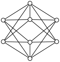
$G_{5\,622}$

Main Eigenvalues: $\frac{1-\sqrt{65}}{2},\frac{1+\sqrt{65}}{2}$
Walk Matrix $3$-walk Matrix $\begin{pmatrix}1&4\\ 1&4\\ 1&4\\ 1&4\\ 1&5\\ 1&5\\ 1&5\\ 1&5\end{pmatrix}$ $\begin{pmatrix}1&4&20\\ 1&4&20\\ 1&4&20\\ 1&4&20\\ 1&5&21\\ 1&5&21\\ 1&5&21\\ 1&5&21\end{pmatrix}$

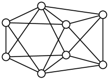
$G_{12\,058}$

Main Eigenvalues: $\frac{3-\sqrt{37}}{2},\frac{3+\sqrt{37}}{2}$
Walk Matrix $3$-walk Matrix $\begin{pmatrix}1&4\\ 1&4\\ 1&4\\ 1&4\\ 1&5\\ 1&5\\ 1&5\\ 1&5\end{pmatrix}$ $\begin{pmatrix}1&4&19\\ 1&4&19\\ 1&4&19\\ 1&4&19\\ 1&5&22\\ 1&5&22\\ 1&5&22\\ 1&5&22\end{pmatrix}$

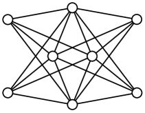
$G_{5\,626}$

Main Eigenvalues: $1+\sqrt{17},1-\sqrt{17}$
Walk Matrix $3$-walk Matrix $\begin{pmatrix}1&4\\ 1&4\\ 1&4\\ 1&4\\ 1&6\\ 1&6\\ 1&6\\ 1&6\end{pmatrix}$ $\begin{pmatrix}1&4&24\\ 1&4&24\\ 1&4&24\\ 1&4&24\\ 1&6&28\\ 1&6&28\\ 1&6&28\\ 1&6&28\end{pmatrix}$

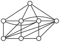
$G_{12\,093}$

Main Eigenvalues: $2+\sqrt{10},2-\sqrt{10}$
Walk Matrix $3$-walk Matrix $\begin{pmatrix}1&4\\ 1&4\\ 1&4\\ 1&4\\ 1&6\\ 1&6\\ 1&6\\ 1&6\end{pmatrix}$ $\begin{pmatrix}1&4&22\\ 1&4&22\\ 1&4&22\\ 1&4&22\\ 1&6&30\\ 1&6&30\\ 1&6&30\\ 1&6&30\end{pmatrix}$

Figure 2: The only two counterexamples on at most $8$ vertices, as described in 3.2.

 

Theorem 3.3.

Let $G$, $H$ be two graphs with $\operatorname{CDC}(G)\simeq\operatorname{CDC}(H)$, and let $k$ be a natural number. Then

$$\mathbf{W}_{G}(k)=\mathbf{W}_{H}(k)$$

for appropriate labelling of the vertices.

Proof.

For a graph $\Gamma$, let $\mathbf{A}_{\Gamma}=\mathbf{A}(\Gamma)$ and $\mathbf{C}_{\Gamma}=\mathbf{A}(\operatorname{CDC}(\Gamma))$. Since $\operatorname{CDC}(G)\simeq\operatorname{CDC}(H)$, we can relabel the vertices of the graph $H$ to get $H^{\prime}$, so that $\mathbf{C}_{G}=\mathbf{C}_{H^{\prime}}$. Now for any $0\leqslant\ell\leqslant k$, we have that

$${\mathbf{C}_{G}}^{\ell}\mathbf{j}=\begin{pmatrix}{\mathbf{A}_{G}}^{\ell}\mathbf{j}\\ \hline\cr{\mathbf{A}_{G}}^{\ell}\mathbf{j}\end{pmatrix}\qquad\text{and}\qquad{\mathbf{C}_{H^{\prime}}}^{\ell}\mathbf{j}=\begin{pmatrix}{\mathbf{A}_{H^{\prime}}}^{\ell}\mathbf{j}\\ \hline\cr{\mathbf{A}_{H^{\prime}}}^{\ell}\mathbf{j}\end{pmatrix},$$

but since $\mathbf{C}_{G}=\mathbf{C}_{H^{\prime}}$, it follows that ${\mathbf{A}_{G}}^{\ell}\mathbf{j}={\mathbf{A}_{H^{\prime}}}^{\ell}\mathbf{j}$ for all $0\leqslant\ell\leqslant k$, so the columns of $\mathbf{W}_{G}(k)$ and $\mathbf{W}_{H}(k)$ are equal. ∎

Counterexample 3.4.

A counterexample establishing that the converse of theorem 3.3 is false is given in figure 3. Indeed, those graphs have

$$\mathbf{W}_{G}=\begin{pmatrix}1&3&9\\ 1&3&10\\ 1&3&10\\ 1&3&10\\ 1&3&10\\ 1&3&9\\ 1&4&12\end{pmatrix}=\mathbf{W}_{H},$$

but $\operatorname{CDC}(G)\nsimeq\operatorname{CDC}(H)$.  

Graph $G$

Graph $H$

Figure 3: Graphs $G$ and $H$ give a counterexample to the converse of theorem 3.3, since they have the same walk matrix but different CDC’s.

Recall that the main eigenspace $\operatorname{Main}(G)$ of a graph $G$ is the subspace generated by the vectors obtained by the decomposition of $\mathbf{j}$ into the eigenspaces of $\mathbf{A}(G)$. An important result about $\operatorname{Main}(G)$ which follows from Vandermonde matrix theory is given in [4] and [5], and states the following.

Theorem 3.5 ([4]).

Let $G$ be a graph with adjacency matrix $\mathbf{A}$. Then the set

$$B=\{\mathbf{j},\mathbf{Aj},\dots,\mathbf{A}^{p-1}\mathbf{j}\}$$

is a set of linearly independent vectors in ${\mathds{R}}^{n}$. Moreover, $B$ forms a basis for $\operatorname{Main}(G)$.

This fact yields the following two corollaries immediately.

Corollary 3.6 ([6]).

Let $G$ be a graph. Then

$$\dim(\operatorname{Main}(G))=p,\qquad\text{and}\qquad\operatorname{rank}\mathbf{W}_{G}(k)=\min\{k,p\}.$$

Corollary 3.7 ([4]).

Let $G$ and $H$ be two graphs with the same walk matrix. Then

$$\operatorname{Main}(G)=\operatorname{Main}(H).$$

iv   Equivalence of Same CDC and TF-Isomorphism

If two graphs $G$, $H$ have isomorphic canonical double coverings, that is, $\operatorname{CDC}(G)\simeq\operatorname{CDC}(H)$, and $G$ is connected, we do not necessarily have that $H$ is connected. Indeed, $\operatorname{CDC}(C_{6})\simeq\operatorname{CDC}(K_{3}\cupdot K_{3})$ as we saw in figure 1.

However, we do have the following.

Lemma 4.1.

Let $G$ and $H$ be two graphs with $\operatorname{CDC}(G)\simeq\operatorname{CDC}(H)$. Then $G$ has no isolated vertices if and only if $H$ has no isolated vertices.

Proof.

Indeed, if $G$ has an isolated vertex, then $G=G^{\prime}\cupdot K_{1}$, so

$$\operatorname{CDC}(G)=\operatorname{CDC}(G^{\prime}\cupdot K_{1})=\operatorname{CDC}(G^{\prime})\cupdot\operatorname{CDC}(K_{1})=\operatorname{CDC}(G^{\prime})\cupdot\macc@depth\char 1\relax\frozen@everymath{\macc@group}\macc@set@skewchar\macc@nested@a 111{K}_{2}$$

by lemma 2.2, and therefore $\operatorname{CDC}(H)=\operatorname{CDC}(G^{\prime})\cupdot\macc@depth\char 1\relax\frozen@everymath{\macc@group}\macc@set@skewchar\macc@nested@a 111{K}_{2}$. Thus the matrix

$$\mathbf{A}(\operatorname{CDC}(H))=\left(\begin{array}[]{c|c}\mathbf{O}&\mathbf{A}(H)\\ \hline\cr\mathbf{A}(H)&\mathbf{O}\end{array}\right),$$

has two whole columns of zeros, corresponding to the isolated vertices which make up $\macc@depth\char 1\relax\frozen@everymath{\macc@group}\macc@set@skewchar\macc@nested@a 111{K}_{2}$. But a column of zeros in the matrix above arises only when a whole column of zeros is present in one of the non-zero blocks $\mathbf{A}(H)$, and since both non-zero blocks are equal to $\mathbf{A}(H)$, then these two columns must be distributed equally among both $\mathbf{A}(H)$’s (otherwise they would be different). In other words, $\mathbf{A}(H)$ must have a column of zeros, and consequently $H$ has an isolated vertex. This argument is symmetric (simply interchange $G$ and $H$) so we also have the converse. ∎

Theorem 4.2.

Suppose $G$ and $H$ are two graphs with adjacency matrices ${\mathbf{A}}_{G}$ and ${\mathbf{A}}_{H}$. Then $\operatorname{CDC}(G)\simeq\operatorname{CDC}(H)$ if and only if there exist two permutation matrices $\mathbf{Q}$ and $\mathbf{R}$ such that

$$\mathbf{Q}\,{\mathbf{A}}_{G}\,\mathbf{R}={\mathbf{A}}_{H}.$$

Proof.

Suppose, without loss of generality, that the graphs $G$ and $H$ have no isolated vertices (if they do, then by lemma 4.1, we could simply pair them off until we are left with two graphs having no isolated vertices). If $\operatorname{CDC}(G)\simeq\operatorname{CDC}(H)$, then there exists a permutation matrix $\mathbf{P}=\left(\begin{smallmatrix}\lx@intercol\hfil$\mathbf{P}_{11}$\hfil\lx@intercol\vrule\lx@intercol&\mathbf{P}_{12}\\[2.0pt] \hline\cr\lx@intercol\hfil\hfil\lx@intercol\vrule\lx@intercol&\\ \lx@intercol\hfil$\mathbf{P}_{21}$\hfil\lx@intercol\vrule\lx@intercol&\mathbf{P}_{22}\end{smallmatrix}\right)$ such that

$$\mathbf{P}{}^{\scalebox{0.6}{T}}\left(\begin{array}[]{c|c}\mathbf{O}&\mathbf{A}_{G}\\ \hline\cr\mathbf{A}_{G}&\mathbf{O}\end{array}\right)\mathbf{P}=\left(\begin{array}[]{c|c}\mathbf{O}&\mathbf{A}_{H}\\ \hline\cr\mathbf{A}_{H}&\mathbf{O}\end{array}\right).$$

Hence by comparing entries, we get that

$$\mathbf{P}_{21}{}^{\scalebox{0.6}{T}}\mathbf{A}_{G}{\mathbf{P}_{12}}+\mathbf{P}_{11}{}^{\scalebox{0.6}{T}}\mathbf{A}_{G}{\mathbf{P}_{22}}=\mathbf{A}_{H}$$ (5)

$$\mathbf{P}_{21}{}^{\scalebox{0.6}{T}}\mathbf{A}_{G}{\mathbf{P}_{11}}=\mathbf{P}_{12}{}^{\scalebox{0.6}{T}}\mathbf{A}_{G}{\mathbf{P}_{22}}=\mathbf{O},$$ (6)

where equation 6 follows since all the matrices have non-negative entries.

Now observe that

$$(\mathbf{P}_{11}+\mathbf{P}_{21}){}^{\scalebox{0.6}{T}}\mathbf{A}_{G}(\mathbf{P}_{22}+\mathbf{P}_{12})=\mathbf{A}_{H}$$

by equations 5 and 6. Now suppose $\mathbf{Q}=(\mathbf{P}_{11}+\mathbf{P}_{21}){}^{\scalebox{0.6}{T}}$ or $\mathbf{R}=\mathbf{P}_{22}+\mathbf{P}_{12}$ is not a permutation matrix. Being the sum of two submatrices of $\mathbf{P}$, this can only happen if a row (and column) are zero. But then $\mathbf{A}_{H}$ will have a row of zeros, corresponding to an isolated vertex in $H$, a contradiction.

Conversely, if $\mathbf{Q}\mathbf{A}_{G}\mathbf{R}=\mathbf{A}_{H}$, then clearly $\mathbf{P}\mathrel{\vbox{\hbox{\scriptsize.}\hbox{\scriptsize.}}}=\left(\begin{array}[]{c|c}\mathbf{O}&\mathbf{Q}\phantom{{}^{\scalebox{0.6}{T}}}\\ \hline\cr\mathbf{R}{}^{\scalebox{0.6}{T}}&\mathbf{O}\end{array}\right)$ defines a permutation matrix, and it is easy to verify that

$$\mathbf{P}{}^{\scalebox{0.6}{T}}\left(\begin{array}[]{c|c}\mathbf{O}&\mathbf{A}_{G}\\ \hline\cr\mathbf{A}_{G}&\mathbf{O}\end{array}\right)\mathbf{P}=\left(\begin{array}[]{c|c}\mathbf{O}&\mathbf{A}_{H}\\ \hline\cr\mathbf{A}_{H}&\mathbf{O}\end{array}\right),$$

as required. ∎

This weakened notion of graph isomorphism, where $\mathbf{Q}\mathbf{A}_{G}\mathbf{R}=\mathbf{A}_{H}$ and the permutation matrices $\mathbf{Q}$ and $\mathbf{R}$ are not necessarily inverses, was first studied by Lauri et al. in [7]. They give a different proof of theorem 4.2 which uses a combinatorial argument. Such graphs are said to be two-fold isomorphic or TF-isomorphic, and we write

$$G\stackrel{{\scriptstyle\text{\scriptsize TF}}}{{\simeq}}H.$$

The pair of permutations $(\mathbf{Q},\mathbf{R})$ is called the TF-isomorphism.

In [7], the authors introduced TF-isomorphisms. They discuss a pair of TF-isomorphic graphs on 7 vertices found by B. Zelinka (figure 4). This is the third out of the 32 pairs we found using Mathematica.

Graph $G$

Graph $H$

Figure 4: The Zelinka example discussed in [7].

v   Establishing the Hierarchy

In this final section, we compare the strength of relationships and similarities between graphs using the results presented above. This establishes a hierarchy depending on their main eigenvalues, main eigenspaces, main eigenvalues, walk matrices, and CDCs.

Figure 5: The hierarchy we present through our results. The symbol $\Rightarrow$ means “implies”, and $\nRightarrow$ means “does not imply”. The combination $\Leftrightarrow$ is short for $\Rightarrow$ and $\Leftarrow$, i.e. “implies and is implied by”, and similarly $\nLeftrightarrow$ is short for $\nRightarrow$ and $\nLeftarrow$, i.e. “does not imply and is not implied by”. The dashed lines which merge at the $\land$ node denote the conjunction of those two results. The dotted lines denote 5.8.

The hierarchy of results is presented in figure 5. That graphs with $\operatorname{CDC}(G)\simeq\operatorname{CDC}(H)$ have the same walk matrix is established in theorem 3.3. That the converse of theorem 3.3 is false, i.e., that having the same walk matrix does not imply we have isomorphic CDC’s, is shown in 3.4. That being TF-isomorphic and having isomorphic CDC’s are equivalent is established by theorem 4.2. Now we start to fill in some of the missing links.

Counterexample 5.1.

In 3.2, two pairs of graphs are given which have the same walk matrix but different main eigenvalues. Here we prove that the converse is also false. The graphs $G$ and $H$ of figure 6 suffice to prove that having the same main eigenvalues does not imply that the graphs have the same walk matrix. Indeed, they both have main polynomial $x(x^{3}-2x^{2}-4x+7)$, but their walk matrices are

$$\mathbf{W}_{G}=\begin{pmatrix}1&2&6&12\\ 1&2&4&10\\ 1&2&4&10\\ 1&2&6&12\\ 1&4&8&24\\ 1&2&6&14\\ 1&2&6&14\end{pmatrix},\qquad\mathbf{W}_{H}=\begin{pmatrix}1&2&6&12\\ 1&3&7&19\\ 1&2&6&14\\ 1&3&7&19\\ 1&2&6&12\\ 1&3&5&15\\ 1&1&3&5\end{pmatrix}.$$

Moreover, their $\operatorname{CDC}$’s are not isomorphic.

Graph $G$

Graph $H$

Figure 6: Graphs $G$ and $H$ have the same main eigenvalues, but have different walk matrices and different $\operatorname{CDC}$’s.

 

In corollary 3.7, we show that having the same walk matrix implies that the main eigenspace is the same. But does this mean the principal main eigenvectors $\{\mathbf{P}_{1}\mathbf{j},\dots,\mathbf{P}_{p}\mathbf{j}\}$ which generate the space are the same?

Counterexample 5.2.

Here we show that this is not the case, i.e., graphs having the same walk matrix do not necessarily have the same principal main eigenvectors. Indeed, the two pairs of graphs in 3.2 (figure 2) have the same walk matrix but different principal main eigenvectors.

The graphs of the first pair $(G_{5\,622},G_{12\,058})$ each have the following two corresponding principal main eigenvectors:

$$G_{5\,622}:\quad \tfrac{1}{8}(-1\pm\sqrt{65},-1\pm\sqrt{65},-1\pm\sqrt{65},-1\pm\sqrt{65},8,8,8,8)$$

$$G_{12\,058}:\quad \tfrac{1}{6}(-1\pm\sqrt{37},-1\pm\sqrt{37},-1\pm\sqrt{37},-1\pm\sqrt{37},6,6,6,6)$$

Clearly the vectors corresponding to $G_{5\,622}$ are not scalar multiples of those corresponding to $G_{12\,058}$, but both separately span the same main eigenspace.  

Thus the leap from eigenvectors to eigenspace is crucial. In fact, it turns out that if two graphs have the same main eigenvectors but different main eigenvalues, they can never have the same walk matrix:

Proposition 5.3.

Let $G$ and $H$ be two graphs with the same main eigenvectors but different main eigenvalues. Then $\mathbf{W}_{G}(k)\neq\mathbf{W}_{H}(k)$ for all $k\geqslant 2$.

Proof.

Let $G$ and $H$ have the same principal main eigenvectors $\{\mathbf{x}_{1},\dots,\mathbf{x}_{p}\}$, but different eigenvalues, $\mu_{1}^{G},\dots,\mu_{p}^{G}$,and $\mu_{1}^{H},\dots,\mu_{p}^{H}$ respectively. Since they are projections onto distinct eigenspaces, they are orthogonal, linearly independent, and $\mathbf{x}_{1}+\cdots+\mathbf{x}_{p}=\mathbf{j}$. Hence the second column of $\mathbf{W}_{G}(k)$ is

$$\mathbf{A}_{G}\mathbf{j}=\sum_{i=1}^{p}\mathbf{A}_{G}\mathbf{x}_{i}=\sum_{i=1}^{p}\mu_{i}^{G}\mathbf{x}_{i}\neq\sum_{i=1}^{p}\mu_{i}^{H}\mathbf{x}_{i}=\sum_{i=1}^{p}\mathbf{A}_{H}\mathbf{x}_{i}=\mathbf{A}_{H}\mathbf{j}$$

since the $\mathbf{x}_{i}$ are linearly independent, as required. ∎

Example 5.4.

5.3 establishes a non-implication. However, even though it is proven in general, we must ensure that it is not vacuously true.

The graphs $G$ and $H$ in figure 7 have the same principal main eigenvectors

$$(\tfrac{1}{2}(-1\pm\sqrt{5}),\tfrac{1}{2}(-1\pm\sqrt{5}),\tfrac{1}{2}(-1\pm\sqrt{5}),\tfrac{1}{2}(-1\pm\sqrt{5}),1,1,1,1),$$

but their walk matrices are

$$\mathbf{W}_{G}=\begin{pmatrix}1&2\\ 1&2\\ 1&2\\ 1&2\\ 1&4\\ 1&4\\ 1&4\\ 1&4\end{pmatrix}\qquad\text{and}\qquad\mathbf{W}_{H}=\begin{pmatrix}1&3\\ 1&3\\ 1&3\\ 1&3\\ 1&6\\ 1&6\\ 1&6\\ 1&6\\ \end{pmatrix}.$$

Indeed, their main eigenvalues are different. The graph $G$ has main eigenvalues $1\pm\sqrt{5}$, whereas $H$ has main eigenvalues $\frac{3}{2}(1\pm\sqrt{5})$.

Graph $G$

Graph $H$

Figure 7: Graphs $G$ and $H$ have the same principal main eigenvectors, but have different walk matrices.

 

On the other hand, the same principal main eigenvalues and eigenvectors yield the same $k$-walk matrix for any $k$, and the proof is identical:

Theorem 5.5.

Let $k\in{\mathds{N}}$, and suppose $G$ and $H$ are two comain graphs with the same principal main eigenvectors. Then

$$\mathbf{W}_{G}(k)=\mathbf{W}_{H}(k).$$

Proof.

Suppose $G$ and $H$ have main eigenvalues $\mu_{1},\dots,\mu_{p}$, and corresponding principal main eigenvectors $\mathbf{x}_{1}\dots,\mathbf{x}_{p}$. We can write $\mathbf{j}$ as $\mathbf{x}_{1}+\cdots+\mathbf{x}_{p}$. Now the $\ell$th column of $\mathbf{W}_{G}(k)$ is the vector $\mathbf{A}_{G}^{\ell-1}\mathbf{j}$, so

$$\mathbf{A}_{G}^{\ell-1}\mathbf{j}=\sum_{i=1}^{p}\mathbf{A}_{G}^{\ell-1}\mathbf{x}_{i}=\sum_{i=1}^{p}\mu_{i}^{\ell-1}\mathbf{x}_{i}=\sum_{i=1}^{p}\mathbf{A}_{H}^{\ell-1}\mathbf{x}_{i}=\mathbf{A}_{H}^{\ell-1}\mathbf{j},$$

i.e., the $\ell$th column of $\mathbf{W}_{H}(k)$. ∎

Finally we elaborate on what is meant by “related walk matrices” in figure 5.

Theorem 5.6.

Let $G$ and $H$ be two graphs. Then $\operatorname{Main}(G)=\operatorname{Main}(H)$ if and only if there is an invertible matrix $\mathbf{Q}$ such that $\mathbf{W}_{G}\mathbf{Q}=\mathbf{W}_{H}$.

Proof.

If $\operatorname{Main}(G)=\operatorname{Main}(H)$, then the column vectors of $\mathbf{W}_{G}$ and $\mathbf{W}_{H}$ form bases for the same space by theorem 3.5. In particular, the columns of $\mathbf{W}_{H}$ can be expressed as a linear combination of those of $\mathbf{W}_{G}$. Indeed, if the $i$th column $\mathbf{c}_{i}$ is $\alpha_{i1}\mathbf{j}+\alpha_{i2}\mathbf{A}_{G}\mathbf{j}+\cdots+\alpha_{ip}{\mathbf{A}_{G}}^{p-1}\mathbf{j}$, then

$$\mathbf{W}_{H}=\begin{pmatrix}|&|&&|\\ \mathbf{c}_{1}&\mathbf{c}_{2}&\cdots&\mathbf{c}_{p}\\ |&|&&|\end{pmatrix}=\begin{pmatrix}|&|&&|\\ \mathbf{j}&\mathbf{A}_{G}\mathbf{j}&\cdots&{\mathbf{A}_{G}}^{p-1}\mathbf{j}\\ |&|&&|\end{pmatrix}\underbrace{\begin{pmatrix}\alpha_{11}&\cdots&\alpha_{1p}\\ \vdots&\ddots&\vdots\\ \alpha_{p1}&\cdots&\alpha_{pp}\end{pmatrix}}_{=\mathbf{Q}}.$$

$\mathbf{Q}$ must be invertible, since otherwise $\operatorname{rank}(\mathbf{W}_{H})\neq p$.

Now for the converse, in $\mathbf{W}_{H}=\mathbf{W}_{G}\mathbf{Q}$ the column vectors of $\mathbf{W}_{G}$ are combined linearly by $\mathbf{Q}$ so they are still members of $\operatorname{Main}(G)$. Since $\mathbf{Q}$ is invertible, none of the columns of $\mathbf{W}_{G}$ become linearly dependent, so they still span all of $\operatorname{Main}(G)$. Thus $\operatorname{Main}(H)=\operatorname{Main}(G)$. ∎

Example 5.7.

An example of graphs having related walk matrices is given in figure 8. These correspond to graphs 31 and 37 from [8], and were pointed out by Jeremy Curmi.^[9]

Graph $G$

Graph $H$

Figure 8: Graphs $G$ and $H$ have related walk matrices.

Indeed, we have

$$\mathbf{W}_{G}=\begin{pmatrix}1&2\\ 1&2\\ 1&2\\ 1&2\\ 1&5\\ 1&5\end{pmatrix}=\begin{pmatrix}1&3\\ 1&3\\ 1&3\\ 1&3\\ 1&4\\ 1&4\\ \end{pmatrix}\begin{pmatrix}1&-7\\ 0&3\end{pmatrix}=\mathbf{W}_{H}\begin{pmatrix}1&-7\\ 0&3\end{pmatrix}=\mathbf{W}_{H}\mathbf{Q}.$$

This same pair of graphs also serves as a counterexample to the following: having the same main eigenspace does not necessarily mean that they have the same main eigenvectors. Indeed, the principal main eigenvectors of $G$ are $(1,1,1,1,\tfrac{1}{4}(1\pm\sqrt{33}),\tfrac{1}{4}(1\pm\sqrt{33})),$ whereas those of $H$ are $(1,1,1,1,\tfrac{1}{4}(-1\pm\sqrt{33}),\tfrac{1}{4}(-1\pm\sqrt{33})).$  

The graphs in example 5.4 (figure 7) also have related walk matrices: $\mathbf{W}_{G}=\left(\begin{smallmatrix}1&0\\ 0&\nicefrac{{2}}{{3}}\end{smallmatrix}\right)\mathbf{W}_{H}$.

We end with a question which, if has a positive answer, would link CDC’s more intimately to their main eigenvalues.

Question 5.8.

Let $G$ and $H$ be two graphs with $\operatorname{CDC}(G)\simeq\operatorname{CDC}(H)$. Do $G$ and $H$ have the same main eigenvalues?

v.i   Finding Graphs with the same CDC

A simple C program was written which made use of the list of non-isomorphic graphs on 8 vertices available on Brendan McKay’s website.^[3] First, the large search space of $\binom{12\,346}{2}=76\,205\,685$ pairs of non-isomorphic graphs was significantly reduced to 1 595 pairs of graphs which are comain using the QR algorithm. This was the most intensive step computationally—it took an ordinary Linux home desktop around 25 minutes. Then another program simply found the $\operatorname{CDC}$’s of each of the graphs which remained, and these were compared pairwise to check for isomorphism. This took around 5 seconds, and produced 32 pairs of non-isomorphic graphs. These included all pairs on less than 8 vertices implicitly, because such pairs appear with isolated vertices added to both (by lemma 4.1).

Even though the algorithm we constructed narrows the search space to consider only graphs which are comain, the list is still exhaustive; because it was determined by brute force that there are no counterexamples to the conjecture implied by 5.8 on at most 8 vertices.

References

[1]
D. M. Cvetković, M. Doob, and H. Sachs.
Spectra of Graphs: Theory and Applications.
Heidelberg : Johann Ambrosius Barth, 3rd edition, 1995.
[2]
D. L. Powers and M. M. Sulaiman.
The walk partition and colorations of a graph.
Linear Algebra and its Applications, 48:145–159, 1982.
[3]
B. D. McKay and A. Piperno.
Practical graph isomorphism, II.
Journal of Symbolic Computation, 60:94–112, 2014.
[4]
I. Sciriha and D. M. Cardoso.
Necessary and sufficient conditions for a hamiltonian graph.
Journal of Combinatorial Mathematics and Combinatorial Computing
(JCMCC), 80:127–150, 2012.
[5]
P. Rowlinson.