Study of a water-graphene capacitor with molecular density functional theory

Abstract

Interfacial molecular processes govern the performances of electrochemical devices. Aqueous electrochemical systems are often studied using classical density functional theory but with too crude approximations. Here we study a water-graphene capacitor, improving the state of the art by the following key points: 1) electrodes have a realistic atomic resolution, 2) a voltage is applied and 3) water is described by a molecular model. We show how the permittivity and the structure of interfacial water change with voltage. The predicted capacitance agrees with molecular dynamics simulations.

The interface between a solution and an electrode is a complex physicochemical system in which both the liquid and the solid properties strongly differ from their bulk ones. For example, X-ray adsorption experiments coupled with ab-initio molecular dynamics study of the water-gold interface revealed an altered structure with respect to the bulk Velasco-Velez et al. (2014). Applying a voltage between electrodes also impacts the local structure and interfacial properties of the liquid Velasco-Velez et al. (2014); Siepmann and Sprik (1995). In the case of an electrolytic solution, ions adopt a complex structure at the electrode giving rise to an electrical double layer (EDL) Merlet et al. (2014).

Since direct experimental measurements are difficult, a lot of our knowledge on the liquid-electrode interface at the molecular level comes from theories and simulations. The simulation of electrochemical systems is further complicated by the necessity to account for the applied potential difference between the two electrodes. In most studies, the adopted strategy is to impose uniform charge densities of opposite sign at each electrode, which is not equivalent to fixing potential. Siepmann and Sprik Siepmann and Sprik (1995); Willard et al. (2008) proposed a more advanced methodology in which each electrode atom bears a Gaussian charge which values are determined to fix the potential to the desired value. It has been reported that using the fixed charge method in Molecular Dynamics (MD) simulations causes a quick and non-physical raising of the temperature while this is not observed with the fluctuating charge method Merlet et al. (2014, 2012). While MD studies provide an efficient toolbox to study electrochemical systems, they are numerically expensive especially when the fluctuating charges method is used. As an example, the recent computation of the capacitance of a device made of two amorphous carbon electrodes immersed in a sodium chloride aqueous solution took several millions CPU hours Simoncelli et al. (2018).

Classical density functional theory (cDFT) is a computationally less demanding alternative which has been intensively used to study electrochemical systems Härtel et al. (2015); Härtel (2017); Henderson et al. (2011); Jiang et al. (2011, 2012); Kong et al. (2015); Lian et al. (2017a, 2016, b); Velasco-Velez et al. (2014); Härtel et al. (2016). However, in these studies three approximations are made: 1) electrode is modeled by a smooth hard wall with no atomic structure, 2) the applied potential is mimicked by fixing opposite and uniform charge distribution on electrodes and 3) water is described either by a hard-sphere fluid Jiang et al. (2012); Lian et al. (2017a), or by a dielectric constant Härtel et al. (2016, 2015); Härtel (2017); Jiang et al. (2011); Lian et al. (2016, 2017b). These three approximations are quite drastic and limit the relevance of simulations to describe realistic systems since: 1) the electrode structure plays a key role in the capacitance Merlet et al. (2013), 2) it has been shown using MD that fixing the charge instead of the potential affects the structure of the adsorbed layer Merlet et al. (2012) and 3) solvation effects also play a major role in the adsorption of ions at the interface Merlet et al. (2012). To address those three points, we propose to use the molecular density functional theory (MDFT) framework to simulate a capacitor consisting of two graphene electrodes separated by pure water at fixed applied potential difference. Graphene is described by an atomistic model while water is modeled by the molecular force field SPC/E.

MDFT has been extensively detailed in previous work Zhao et al. (2011); Jeanmairet et al. (2013a); Ding et al. (2017); Jeanmairet et al. (2019) and we only briefly recall its basics. In MDFT, a liquid (here water) is described by its density field $\rho(\bm{r},\bm{\Omega})$, which measures the average number of solvent molecules with orientation $\bm{\Omega}$ at a given position $\bm{r}$. For any external perturbation (here the presence of electrodes), it is possible to write a unique functional $F$ of the density. This functional is usually split into the sum of three terms:

$$F[\rho]=F_{\text{id}}[\rho]+F_{\text{ext}}[\rho]+F_{\text{exc}}[\rho].$$ (1)

The ideal term $F_{\text{id}}$ corresponds to the usual entropic term for a non-interacting fluid. The second term $F_{\text{ext}}$ is due to the external potential $V_{\text{ext}}$ of the electrodes acting on the liquid:

$$F_{\text{ext}}[\rho]=\iint\rho\left(\bm{r},\bm{\bm{\Omega}}\right)V_{\text{ext}}(\bm{r},\bm{\Omega})d\bm{r}d\bm{\Omega}$$ (2)

Here, $V_{\text{ext}}$ is the sum of a Lennard Jones potential $V_{\text{ext,LJ}}$ and of an electrostatic term $V_{\text{ext,e}}$ due to interactions between partial charges of water molecules and the fluctuating charges on the electrodes. Finally, the last term of Equation 1 represents the solvent-solvent contribution for which we employ the most accurate expression for SPC/E Ding et al. (2017), which corresponds to the so-called hypernetted chain or equivalently bulk reference fluid approximation.

The density $\rho_{\text{eq}}$ minimizing the functional of Equation 1 is the Grand Canonical equilibrium solvent density of the liquid. This density $\rho_{\text{eq}}$ is inhomogeneous and thus generates an inhomogeneous charge distribution

$$\rho_{c}(\bm{r})=\iint\rho_{\text{eq}}(\bm{r}^{\prime},\bm{\Omega})\widetilde{\rho_{c}}(\bm{r}-\bm{r}^{\prime},\bm{\Omega})d\bm{r}^{\prime}d\bm{\Omega}.$$ (3)

where $\widetilde{\rho_{c}}(\bm{r},\bm{\Omega})=\sum_{i}q_{i}\delta(\bm{r}-\bm{r}_{i_{\bm{\Omega}}})$ is the charge distribution of a single water molecule located at the origin with an orientation $\bm{\Omega}$ , $\delta$ denotes the Dirac distribution, the sum runs over the solvent sites, $q_{i}$ is the charge of site $i$ and $\bm{r}_{i_{\bm{\Omega}}}$ is the position of this site when the molecule has an orientation $\bm{\Omega}$. This inhomogeneous charge distribution polarizes the two electrodes.

To account for the polarizability of electrodes under a fixed potential difference, we employ the method proposed by Siepmann and Sprik. Each electrode atom $j$ bears a Gaussian charge distribution of fixed width 0.505 Å and magnitude $q_{j}$. These charges are treated as additional degrees of freedom and are determined to ensure that the electrostatic potential $V_{j}$ experienced by each carbon atom equals a prescribed value $V_{j,0}=\pm V_{0}$. In practice this is done similarly to previous work Siepmann and Sprik (1995); Willard et al. (2008), by minimizing the functional

$$E_{\text{e}}^{\text{tot}}=E_{\text{e}}-\sum_{j}q_{j}V_{j,0},$$ (4)

with respect to the charges $q_{j}$ where $E_{\text{e}}$ is the electrostatic energy. This set of electrode charges $q_{j}$ creates an electrostatic field $V_{\text{ext,e}}$ in the external potential of Equation 2, which in turn modifies the polarization of the liquid.

To obtain the equilibrium solvent density and the electrode charges we perform successive functional minimizations and electrode charges optimizations as schematized in Figure 1. Initially, we optimize the charges in the absence of solvent and compute the electrostatic potential $V_{\text{ext,e}}$ it induces on each node of the MDFT grid. This potential is then added to the Lennard Jones potential $V_{\text{ext,LJ}}$ of the electrode atoms to compute the external potential $V_{\text{ext}}$ entering Equation 2. After minimization of the functional, the equilibrium solvent charge density $\rho_{c}$ of water is obtained from Equation 3. It contributes to the total electrostatic potential energy $E_{\text{e}}$ in Equation 4, which is minimized to compute a new set of electrode charges. This process is iterated until a convergence criterium is reached, typically when the relative total charge variation between two iterations is below $5.0\ 10^{-4}$.

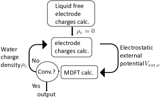
Figure 1: Workflow to compute the equilibrium solvent density and the charge distribution within the electrodes under a fixed potential difference.

We study an electrochemical cell made of two graphene electrodes separated by pure water. Each electrode made of 112 fixed carbon atoms has a surface area of $17.36\times 17.18\ \textrm{\r{A}}^{2}$. The two electrodes are separated by $60\ \textrm{\r{A}}$. We run two sets of simulations. In the first one water is described explicitly using fixed-potential Molecular Dynamics, while in the second one we use the fixed-potential MDFT described above. We run simulations with applied potential differences $\Delta V$ of 0.0, 0.54, 1.1, 1.6 and 2.2 V. The force field parameters are common to both setup: water is described by the SPC/E rigid model and carbon atoms are modeled by a Lennard-Jones site with $\sigma=3.37\ \textrm{\r{A}}$ and $\epsilon=0.23\$kJ.mol^-1 Cole and Klein (1983). The parameters for carbon-water interaction are obtained using the Lorentz-Berthelot mixing rules. Carbon atoms also bear fluctuating Gaussian charges interacting elecrostatically with water.

The MD simulations are preformed in the canonical ensemble at 298 K and the inter-electrode space is filled with 560 water molecules in order to recover the density of the homogeneous fluid ($0.033\ \textrm{\r{A}}^{-3}$) at the center of the cell. Since MDFT is a grand-canonical theory, the number of water molecules is not an input parameter of the simulation but rather a result from it. The predicted number of water molecules is $560\pm 1$ for all values of the applied potential. In MD, the time step is 1 fs and statistics are accumulated for at least 400 ps after 50 ps of equilibration.

Periodic boundary conditions (PBC) are only applied in the $x$ and $y$ directions, i.e parallel to the electrodes. In MDFT, the excess solvent-solvent term is computed through the use of discrete Fourier transform implying a 3D spatial periodicity. To be consistent with the 2D-PBC of the external potential we suppress the undesired periodicity along the $z$-axis by doubling the box size in this direction and imposing a vanishing density by adding an infinite external potential when $z>60\ \textrm{\r{A}}$.

We first examine the in-plane-averaged equilibrium densities of the H and O sites of water along the $z$ direction, defined as

$$n_{\text{A}}(z)=\frac{1}{L_{x}L_{y}}\iint\frac{\rho_{\text{A}}(\bm{r},\bm{\Omega})}{\rho_{\text{A}}^{\text{bulk}}}dxdyd\bm{\Omega}$$ (5)

where $L_{x}$ and $L_{y}$ are the dimensions of the box in the $x$ and $y$ directions, $\rho_{\text{A}}$ is the 3D density of oxygen or hydrogen and $\rho_{\text{A}}^{\text{bulk}}$ is the corresponding density in the bulk solvent. In MD this quantity can be computed through binning of the particles positions.

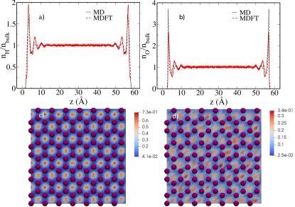
Figure 2: Top: In-plane-averaged equilibrium densities of H (a) and O (b) of water along the $z$ direction. The MD results are in full red and the MDFT results are in dashed black. Bottom: Slices of oxygen density computed by MDFT (c) and MD (d) located at $z\approx 2.5\ \textrm{\r{A}}$, the purple balls represent the graphene carbon atoms.

Figure 2 compares $n_{\text{H}}$ and $n_{\text{O}}$ computed with MD and MDFT for $\Delta V=0.0\ \text{V}$ (oxygen densities for other values of applied voltage are given in supplementary materials). Both density profiles are symmetric with respect to the center of the cell since the two electrodes are identical; applying a non-zero potential difference breaks this symmetry as illustrated in SM. The two methods give results in qualitative agreement with two marked solvation peaks beyond which the homogeneous densities are quickly recovered. A closer look reveals some discrepancies. For the oxygen density in Figure 2.a, the maximum of the first peak is located at $3.0\ \textrm{\r{A}}$ with MDFT, slightly closer to the electrode than with MD ($3.2\ \textrm{\r{A}}$). This first pick is also sharper in MDFT than in MD. These results are consistent with previous work showing that MDFT tends to predict over-structured solvation shells around hydrophobic solutes Jeanmairet et al. (2013b). For the hydrogen density profile in Figure 2.b, the agreement is also qualitative since MDFT tends to predict slightly less structured solvation shells: The two main peaks of the density profile are smaller than in MD.

Despite those differences the agreement between MD and MDFT is good, as confirmed by the 3D densities. In Figure 2 c-d we present the oxygen densities in planes perpendicular to the electrode located at $z\approx 2.5\ \textrm{\r{A}}$. Note that if the two figure are extremely similar, the legend differ. Both methods predict an higher density at the center of the hexagonal ring of graphene and lower density on top of the carbon-carbon bonds. As evidenced in Figure 2.c-d, the MDFT is well defined, while the MD densities, computed after 9 ns of simulation would require more sampling to be fully converged. The effect of the evolution of the density with the sampling time is given in SM.

We now turn to the performance of the water capacitor. Figure 3 displays the charge density $\sigma$ on the positive electrode as a function of the applied potential difference. Of course, the negative electrode bears an opposite charge density. With both methods the charge density varies linearly with the applied potential, which implies a constant value of the differential capacitance over the range of studied applied potentials. Capacitances are computed through linear regression of the data, with the results $C=5.0\$µF.cm^-2 for MD and $C=4.2\ \text{}$µF.cm^-2 for MDFT.

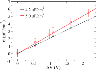
Figure 3: Surface charge density on the positive electrode as a function of the applied potential difference. The MD results are the red square and the error bars represent the standard deviation. MDFT results are the black circles. The solid red line and the dashed black line are linear fits of the data. The corresponding slopes are the capacitances

Knowing the charge distribution on each electrode, it is possible to sum it with that of the solvent computed through Equation 3 to obtain the total charge distribution in the cell. This allows to compute the evolution of the potential across the cell by solving the Poisson Equation

$$\Delta\Psi(z)=-\frac{\bar{\rho_{c}}(z)}{\epsilon_{0}},$$ (6)

where $\bar{\rho_{c}}$ is the in-plane averaged total charge distribution and $\epsilon_{0}$ is the vacuum permittivity. The Poisson potential profiles computed with MDFT are displayed in Figure 4. This potential is constant within the electrode. It then drops at the interface and oscillates in a region of approximately 14 Å with respect to the electrode before exhibiting a linear behavior characteristic of a bulk dielectric material submitted to an external electric field. The oscillation results from the layering of water at the interface as observed in the density profiles of Figure 2. Except for the short-circuit case ($\Delta V=0.0\ \text{V}$) the potential is non symmetric because of different organizations of the water molecules at the positive and negative electrodes, as is discussed later. To compute the dielectric constant of water, we first calculate the total charge density $\sigma_{L}$ (resp. $\sigma_{R}$) of adsorbed water layers on the left (resp. right) electrode by integrating the charge density of the solvent in the region of the cell $z<20\ \textrm{\r{A}}$ (resp $z>40\ \textrm{\r{A}}$). We then measure the potential drop $\Delta\Psi$ across the region between the planes at $z=20\ \textrm{\r{A}}$ and $z=40\ \textrm{\r{A}}$ in Figure 4. This allows to compute the surface capacitance $C$ due to the dielectric liquid with the relation $\sigma_{L}=C_{S}\Delta\Psi$ for the different values of the applied potential. For a capacitor composed of two planar metallic plates separated by a dielectric medium the surface capacitance reads:

$$C_{S}=\frac{\epsilon_{r}\epsilon_{0}}{d}$$ (7)

with $d$ the distance between the two plates and $\epsilon_{r}$ the permittivity of the dielectric medium. Results for the permittivity $\epsilon_{r}$ are presented in Table 1 for different values of applied potential.

At low voltage, we obtain a value of $\epsilon_{r}=68.1$ in agreement with previous values computed by MD by several groups Yeh and Berkowitz (1999); Apol et al. (2002); Zhang and Sprik (2016). When the applied potential increases, the computed dielectric constant decreases, which is a known effect due to saturation of the dielectric material Yeh and Berkowitz (1999); Willard et al. (2008).

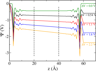
Figure 4: Poisson potential across the cell computed using Equation 6 for different values of the applied voltage $\Delta V$

$\Delta V$ (V)	$\epsilon_{r}$
0.54	68.1
1.1	67.3
1.6	63.0
2.2	60.3

Table 1: Dielectric constant of SPC/E water computed for different values of the applied voltage $\Delta V$.

Looking more closely at the evolution of the Poisson potential across the two interfaces, we observe different behaviors at the two electrodes. On the positive electrode (left), increasing the applied voltage $\Delta V$ simply enhances the potential drop observed at $0.0\ V$. On the negative electrode (right), we observe a change of sign in the evolution of the Poisson potential across the interface as the voltage increases. In order to understand the molecular origin of this phenomenon we report in Figure 5, the planar-averaged $z$ component of the molecular dipolar polarization of the solvent, defined as:

$$\cos\theta_{z}=\iiint\frac{\rho(\bm{r},\bm{\Omega})\bm{\Omega}\cdot\bm{e}_{z}}{\rho(\bm{r},\bm{\Omega})}dxdyd\bm{\Omega}.$$ (8)

With the dipolar moment of a water molecule $\mu_{0}$ added as a prefactor, the numerator of Equation 8 corresponds to the $z$-component of the water dipolar polarization field. Thus, $\cos\theta_{z}$ gives information about the average orientation of water molecules located at a given $z$: When $\cos\theta_{z}=1$ the dipole of water molecule, pointing from oxygen to the center of mass of hydrogen, is aligned with the $z$ axis. There are clearly some preferential orientation of water with respect to the $z$ axis for all values of the applied potential. We computed similarly $\cos\theta_{x}$ and $\cos\theta_{y}$ but no preferential orientation was observed.

At $\Delta V=0.0\ \text{V}$, $\cos\theta_{z}$ is symmetric with respect to the center of the cell. As expected, water molecules organize identically at the two sides of the cell, and the oxygen are lying closer to the surface than the hydrogen. Note that a purely dipolar model (such as the Stockmayer fluid) would not polarize. The observed finite and structured polarization emerges from the geometrical structure of the water molecules, leading to a density-polarization density coupling, that is fully accounted for in our molecular DFT approach Jeanmairet et al. (2016).

When the potential difference is increased, we observe a different behavior of the polarization on each electrode. On the positive electrode (left), increasing the potential enhances the oscillation of polarization with respects to $\Delta V=0.0\ \text{V}$ and the global orientation of water molecules at the interface is not modified. On the negative electrode (right), we observe a flip of sign in the first peak of polarization for voltage larger than $1.1\ V$, accompanied with a slight shift of the position of this maximum toward the surface. This indicates that for large enough voltage the preferential orientation of adsorbed molecules is modified, as they flip with the hydrogen atoms pointing toward the surface.

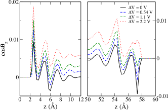
Figure 5: Average molecular polarization $\cos\theta_{z}$ along the normal to the electrode surface.

In summary, this paper reports a MDFT study of an electrochemical device. Compared to other classical DFT calculations of similar systems, this work introduce three major improvements: 1) the electrodes are described by a realistic atomistic model, 2) the calculations are done at fixed potential difference and 3) water is described by the realistic molecular SPC/E model. Our implementation was tested on a graphene-water capacitor and compared to fixed potential MD for thorough validation. The solvation structure is almost quantitatively predicted by MDFT. The prediction of the capacitance of the device is good and the computed dielectric permittivity of the SPC/E water model for different values of the applied potential difference agrees well with previous MD simulations. It was also possible to take advantage of the 3D resolution of the equilibrium solvent density to gain precise insight into the orientational order of water at the interface and its evolution with the applied potential difference. In this paper, functional minimization and the electrode charge optimization were carried out independently and sequentially. It should be possible to propose a functional form depending on both the solvent density and the electrode charges. Minimizing such a functional would allow to find the equilibrium solvent density and the equilibrium electrode charge distribution self consistently. This is a current direction of research. The limitations of MDFT in the straight HNC approximation considered here, especially close to mildly charged entities, have already been pinpointed and so-called « bridge » functionals going beyond HNC have been suggested Levesque et al. (2012); Jeanmairet et al. (2013b, 2015). Inclusion of those in the present problem is a direction of investigations.