Triplet Leptogenesis, Type-II Seesaw Dominance, Intrinsic Dark Matter, Vacuum Stability and Proton Decay in Minimal SO(10) Breakings

Abstract

We implement type-II seesaw dominance for neutrino mass and baryogenesis through heavy scalar triplet leptogenesis in a class of minimal non-supersymmetric SO(10) models where matter parity as stabilising discrete symmetry as well as WIMP dark matter (DM) candidates are intrinsic predictions of the GUT symmetry. We also find modifications of relevant CP-asymmetry formulas in such models. Baryon asymmetry of the universe as solutions of Boltzmann equations is further shown to be realized for both normal and inverted mass orderings in concordance with cosmological bound and best fit values of the neutrino oscillation data including $\theta_{23}$ in the second octant and large values of leptonic Dirac CP-phases. Type-II seesaw dominance is at first successfully implemented in two cases of spontaneous SO(10) breakings through SU(5) route where the presence of only one non-standard Higgs scalar of intermediate mass $\sim 10^{9}-10^{10}$ GeV achieves unification. Lower values of the SU(5) unification scales $\sim 10^{15}$ GeV are predicted to bring proton lifetimes to the accessible ranges of Super-Kamiokande and Hyper-Kamiokande experiments. Our prediction of WIMP DM relic density in each model is due to a $\sim{\cal O}(1)$ TeV mass matter-parity odd real scalar singlet ($\subset{16}_{H}\subset$ SO(10)) verifiable by LUX and XENON1T experiments. This DM is also noted to resolve the vacuum stability issue of the standard scalar potential. When applied to the unification framework of M. Frigerio and T. Hambye, in addition to the minimal fermionic triplet DM solution of $2.7$ TeV, our mechanism of type-II seesaw dominance and triplet leptogenesis is also found to make an alternative prediction of the triplet fermion plus the real scalar singlet DM near the TeV scale.

^∗∗email:mainak.chakraborty2@gmail.com
^∗email:minaparida@soa.ac.in
^†email:sahoobiswonath@gmail.com

1 Introduction

Despite the success of standard model (SM) paradigm based upon $SU(2)_{L}\times U(1)_{Y}\times SU(3)_{C}(\equiv G_{213})$ including the evidence of Higgs boson [1], the model fails to explain several issues like neutrino oscillation [2, 3, 4], baryon asymmetry of the universe (BAU) [5, 6], nature of dark matter (DM) and its stability [7, 8], the vacuum stability of scalar potential, and the origin of disparate values of gauge couplings. Out of Grand unified theories (GUTs) [9, 10, 11, 12, 13] suggested to alleviate issues confronting the SM supersymmetric (SUSY) GUTs [14, 15, 16] have been considered to be quite fundamental in understanding the stability of the standard model vacuum and the origin of three forces of nature. SUSY SO(10)[11] predicts R-Parity [17, 18, 19] for stability of dark matter candidates, explains the origin of experimentally observed parity violation in weak interaction [9, 20, 21, 22, 23] , and more interestigly it predicts the combined type-I [24, 25] plus type-II [26, 27, 28, 29, 30] hybrid seesaw formula [31, 32] for neutrino mass matrix $m_{\nu}$. Among a large number of investigations in neutrino physics[33], SUSY GUTs with type-II seesaw dominance have the special advantage [34] that the observed pattern of quark and lepton mixings at low energies can be explained without using any flavor symmetry [35, 36] from the fact that the b-quark and the $\tau$-lepton masses are nearly equal at the GUT scale [37].

However, in the absence of any experimental evidence of SUSY, very recently non-SUSY SO(10) has been in the spot light because of its inherent and intrinsic capability to predict DM candidates and their stability. In particular, an intrinsic gauged discrete symmetry [38], surviving as matter parity in SO(10) breakings [39, 40, 41, 42, 43, 44, 45, 46, 47]

$$Z_{\rm MP}={(-1)}^{3(B-L)},$$ (1)

has been found to stabilise the non-standard scalars and fermions which are also predicted to originate intrinsically from this non-SUSY GUT representations as possible DM candidates leading to a number of attractive predictions [39, 40, 41, 42, 43, 44, 45, 46, 47]. It is quite interesting to note that the matter parity conservation down to low energies naturally emerges whenever the popular Higgs representation ${126}_{H}$ is used to break the underlying $U(1)_{B-L}$ gauge symmetry and ${10}_{H}$ is used to break the electroweak symmetry materialising in type-I$\oplus$type-II seesaw formula for neutrino masses discussed in Sec.4. So far the SO(10) based matter parity conserving DM models have been largely exploiting the type-I seesaw dominance in non-SUSY SO(10) [39, 40, 41, 44, 45, 47]. On the other hand it is interesting to note that whenever type-II dominance occurs in a minimal SUSY or non-SUSY SO(10) GUT, it predicts the following constraint relation among mass eigen values $m_{i}$($M_{N_{i}}$) of left-handed (right-handed) neutrinos

$$m_{1}:m_{2}:m_{3} :: M_{N_{1}}:M_{N_{2}}:M_{N_{3}}.$$ (2)

All neutrino mass generation mechanisms are also expected to respect the cosmological bound [6] $\sum_{i}{\hat{m}}_{i}\leq 0.23\,\,{\rm eV}.$

Alternative to RHN decay leptogenesis in SM extensions[48], interesting models of triplet leptogenesis have been also proposed [49, 50, 51, 52, 53] where the heavy scalar triplet $\Delta_{L}(3,-1,1)$ decay generates the desired CP-asymmetry that leads to baryogenesis through sphaleron interaction [54] near the electroweak scale. With such nontrivial constraints and the triplet leptogenesis requirement [50, 51, 53] that one of the heavy neutrinos mediating the loop for CP-asymmetry generation should be around the $\Delta_{L}$ mass, in the present work we find that the triplet leptogenesis theory [50, 51] is ideally suited for a general class of three different non-SUSY SO(10) models. This class of models with SM paradigm, besides successfully generating BAU, also explains neutrino oscillation data via type-II seesaw dominance and predicts matter parity stabilised weakly interacting massive particle (WIMP) [55] dark matter from within the non-SUSY SO(10) consistent with precision unification of gauge couplings leading to verifiable proton decay. These models are further noted to resolve the issue of vacuum stability of the SM Higgs potential. In the presence of type-II seesaw dominance in matter parity conserving SO(10) breakings, we further find modifications of relevant CP-asymmetry formulas of [50, 51, 53] based upon SM extensions. These objectives have been realized through type-II seesaw dominance induction in a general class of three non-SUSY SO(10) Models: (i) Model-I with $\kappa(3,0,8)$- unification framework, (ii) Model-II with $\eta(3,-1/3,6)$- unification framework, and (iii) Model-III with Frigerio-Hambye type unification framework [41].
Our successful realization of heavy triplet leptogenesis consistent with $\theta_{23}$ in the second octant, large Dirac phases and other neutrino mixings in concordance with most recent neutrino oscillation data [4] uncovers a new set of important results in the area of thermal leptogenesis. This is especially so in view of an interesting recent conclusion that strongly thermal SO(10)-inspired leptogenesis (through type-I seesaw) can be hardly compatible with atmospheric neutrino mixing angle in the second octant [56, 57].
Highlights of this work are

• Implementation of Type-II seesaw dominance and precision coupling unification in a class of three different non-SUSY SO(10) breakings to SM via SU(5) route with only the scalar singlet/fermionic triplet dark matter at the TeV scale verifiable by LUX and XENON1T experiments.

• Precision coupling unification ensured by the presence of a single nonstandard scalar/fermionic multiplet of intermediate mass $\sim 10^{9.2}-10^{10.4}$ GeV [47, 41] and type-II dominance ensured by higher scale insertion of a complete ${15}_{H}\subset$ SU(5) at $M_{\Delta}$ with much larger SO(10) unification scale, $M_{SO(10)}\gg M_{SU(5)}>M_{\Delta}$.

• Lower values of SU(5) GUT scale, $M_{SU(5)}\sim 10^{15}$ GeV, triggering verifiable proton decay by Super-Kamiokande and Hyper-Kamiokande search experiments [58, 59] in all the three models.

• Prediction of a class of new CP-asymmetry formulas for leptogenesis compared to existing models [50, 51, 53] in minimal matter parity conserving SO(10) breakings in the presence of type-II seesaw dominance.

• First successful minimal non-SUSY SO(10) realization of baryogenesis via heavy scalar triplet decay leptogenesis with the $\Delta_{L}-$ dilepton coupling matrix determined from best fit values of the neutrino oscillation data in concordance with both normally ordered (NO) and invertedly ordered (IO) masses with $\theta_{23}$ in the second octant including large Dirac CP-phases.

• These realizations of type-II seesaw and heavy triplet decay thermal leptogenesis with $\theta_{23}$ in the second octant to be contrasted with SO(10)-inspired strongly thermal RHN decay leptogenesis which are hardly compatible with atmospheric mixing angle in the second octant [56, 57].

• Intrinsic matter parity stabilised TeV mass real scalar singlet ansatz for both WIMP DM relic density and SM scalar potential vacuum stability verifiable by LUX and XENON1T.

• Results indicating non-SUSY SO(10) as self sufficient theory for neutrino masses, baryon asymmetry, dark matter, vacuum stability of SM scalar potential, origin of three gauge forces, and observed proton stability.

• All other predictions remaining similar to Model-I and Model-II, two different paths for TeV scale DM through Model-III utilizing Frigerio-Hambye type unification framework [41]:

  1. Triplet fermionic DM mass same as $m_{\Sigma}\sim 2.7$ TeV in the minimal scenario of [41], a new heavy Higgs scalar singlet of intermediate mass ($=10^{9}$ GeV) resolves the vacuum stability issue by threshold effects on Higgs quartic coupling [60].
     

  2. A combined DM scenario comprising of both the fermionic triplet and real scalar singlet near TeV scale in concordance with LUX and XENON1T bounds. In this case the non-perturbative Sommerfeld enhancement effect can be dispensed with.

This work is organized in the following manner. In Sec.2 we discuss gauge coupling unification and GUT scale predictions in new models of type-II seesaw dominance emerging from matter parity conserving minimal non-SUSY SO(10) breakings. Prediction of the light real scalar singlet DM is also noted in this section with necessary derivation. Proton lifetime predictions including GUT threshold effects have been discussed in Sec.3. In Sec.4 we discuss neutrino mass fitting by type-II seesaw dominated formula and derivation of relevant Yukawa couplings as inputs to leptogenesis. Our predictions on WIMP DM and resolution of vacuum stability are discussed in Sec.5. Solutions to vacuum stability problem in the triplet fermionic DM model and its modification are discussed in Sec. 6. Baryogenesis via heavy scalar triplet decay is discussed in Sec.7. We summarize and conclude in Sec.8.

2 Type-II Seesaw Dominance Models from Non-SUSY SO(10)

2.1 New TeV Scale Non-SUSY Dark Matter Models

For type-II seesaw dominance in SUSY SO(10) two essential ingredients have been suggested [61]: (i). SUSY SO(10) must break into minimal supersymmetric standard model (MSSM) in two steps: SUSY SO(10) $\to$ SUSY SU(5) $\to$ MSSM with the mass scale in the first step being heavier enough than the SUSY SU(5) breaking scale: $M_{SUSYSO(10)}>>M_{SUSYSU(5)}$, (ii). To maintain pre-existing SUSY unification, the fine-tuned mass of the full Higgs multiplet ${15}_{H}\subset$ SU(5) containing the LH triplet $\Delta_{L}(3,-1,1)$ must be lighter than the SUSY unification scale. Clearly the implementation needs MSSM like TeV scale particle spectrum [15] and the SUSY GUT scale of eq.(3) derived from RG extrapolation of the CERN-LEP data [16].

$$M_{SUSY\,SU(5)}\sim 10^{16}{\rm GeV},$$ (3)

In purely non-SUSY SM paradigm, the well known failure of coupling unification is restored [43, 62] through a TeV scale particle spectrum which is the MSSM spectrum minus the superpartners

$$\phi^{S}_{1}(2,1/2,1),\phi^{S}_{2}(2,-1/2,1),\phi^{F}_{1}(2,1/2,1),\Phi_{2}^{F}(2,-1/2,1),\,\,$$

$$F_{\sigma}(3,0,1),F_{8}(1,0,8)$$ (4)

where $\phi^{S}_{1}(2,1/2,1),\phi^{S}_{2}(2,-1/2,1)$ represent two scalars of a two-Higgs doublet model. In the SO(10) context [43] $\phi^{S}_{1}\subset{10}_{H}$, $\phi^{S}_{2}\subset{16}_{H}$, $\phi^{F}_{1,2}\subset{10}_{F}$ and $(F_{\sigma},F_{8})\subset{45}_{F}$ of SO(10). In attributing non-SUSY SU(5) origin of scalar doublet DM and radiative seesaw [63], a somewhat different TeV scale spectrum has been also suggested [64]. In the absence of any evidence in favour of SUSY [65] or MSSM like TeV spectrum of eq.4, in this work we complete unification for type-II seesaw dominance through only one non-standard scalar $\kappa(3,0,8)$ as in Model-I, or $\eta(3,-1/3,6)$ as in Model-II. In Model-III we implement type-II seesaw dominance using unification framework of [41] where a fermionic triplet DM $\Sigma_{F}(3,0,1)$ of mass 2.7 TeV has been suggested. A real scalar singlet dark matter $\chi_{S}^{R}(1,0,1)$ is predicted to complete vacuum stability in all the three models. Thus, in contrast to the extended particle spectrum of eq.(4), our TeV scale particles accessible to LUX and XENON1T are

$$\chi_{S}^{R}(1,0,1)\,\,{\rm OR}\,\,{\Sigma_{F}(3,0,1)}.\,\,$$ (5)

All the three models also predict one order lighter unification scale

$$M_{SU(5)}\simeq 10^{15}\,\,{\rm GeV}$$ (6)

with corresponding reduction in proton lifetime accessible to Super-Kamiokande and Hyper-Kamiokande [58, 59].

2.1.1 General Considerations with Matter Parity

In SM extended theories [8] the candidates of DM are externally added with an ad-hoc assumption on their stabilising discrete symmetry. Such theories are naturally expected to be incomplete in the absence of any fundamental origin of such DM candidates and their stabilising symmetry.

But in non-SUSY $SO(10)$ this stabilising symmetry [38, 39, 40] called matter parity ($Z_{MP}$) defined through eq.(1) of Sec.1), automatically emerges as intrinsic gauged discrete symmetry whenever the neutral component of the right-handed (RH) Higgs triplet $\Delta_{R}(1,3,-2,1)\subset{126}_{H}$ of SO(10) is assigned appropriate VEV to break $SU(2)_{R}\times U(1)_{B-L}$ gauge symmetry leading to the SM Lagrangian either directly or through intermediate left-right gauge symmetries[42, 43, 44, 45, 46], or through SU(5) route. Here the quantum numbers of RH Higgs triplet $\Delta_{R}(1,3,-2,1)$ are defined under left-right gauge symmetry $SU(2)_{L}\times SU(2)_{R}\times U(1)_{B-L}\times SU(3)_{C}$ ($\equiv G_{2213}$)[20]. Such breakings also enable to identify the SO(10) representations with odd value of matter parity $Z_{MP}=-1$ for $16$, $144$,$560$,….but with even value of $Z_{MP}=+1$ for $10$, $45$, $54$, $120$, $126$, $210$, ${210}^{\prime}$,$660$ ….. Then it turns out that the would-be DM scalars are predicted to be in the non-standard scalar representations ${16}_{H},{144}_{H}...$ while the DM fermions are predicted to be in the non-standard fermionic representations ${10}_{F},{45}_{F},{54}_{F},{120}_{F},{126}_{F},{210}_{F}$….. of even matter parity. All the SM fermions contained in the spinorial representation ${16}_{F}$ of SO(10) thus possess odd matter parity $Z_{MP}=-1$ while the standard model Higgs contained in ${10}_{H}$ carries even value of $Z_{MP}=+1$. All the models discussed below rely upon the spontaneous symmetry breaking pattern

$$SO(10)\longrightarrow SU(5)\times U(1)_{X}\longrightarrow SU(5)\longrightarrow SM.$$ (7)

where

$$X=4T_{3R}+3(B-L).$$ (8)

In eq.(8) $T_{3R}=$ third component of RH isospin and $B-L=$ baryon minus lepton number. We will assume the two large mass scales for the first two-steps to be identical to $M_{SO(10)}$ so that no generality is lost by considering the effective symmetry breaking chain

$$SO(10)\longrightarrow SU(5)\longrightarrow SM.$$ (9)

For the sake of utilisation in Model-I, Model-II and Model-III discussed below we need the following SO(10) branching rules [66]

SO(10) $\supset$ SU(5)$\times U(1)_{X}$:

$${210}_{H}=[\Omega=1_{H}(0)]+{75}_{H}(0)+{24}_{H}(0)+....,$$

$${45}_{H}=1_{H}(0)+{24}_{H}(0)++{10}_{H}(4)+{\overline{10}}_{H}(-4)+...,$$

$${126}_{H}=[\Delta^{0}_{R}=1_{H}(-10)]+{\overline{50}}_{H}(2)+{15}_{H}(6)+...,$$

$${16}_{H}=[\chi_{S}=1_{H}(-5)]+{10}_{H}(-1)+{\overline{5}}_{H}(3)....,$$

$${10}_{H}=5_{H}(2)+{\overline{5}_{H}}(-2)+....$$ (10)

The SU(5) singlet $1_{H}\subset{126}_{H}$ noted above is the neutral component of the right-handed (RH) triplet $\Delta_{R}(1,3,-2,1)$ under $G_{2213}$ [20]. The left-handed (LH) scalar triplet $\Delta_{L}(3,1,-2,1)$ responsible for type-II seesaw and the RH triplet $\Delta_{R}(1,3,-2,1)$ that generates RHN masses through its $U(1)_{X}$ breaking VEV are noted to originate from the same representation ${126}_{H}$. We further need the following branching rules for SU(5)$\supset$ SM

SU(5) $\supset SU(2)_{L}\times U(1)_{Y}\times SU(3)_{C}(=G_{213})$:

$${5}_{H}=\phi(2,1/2,1)+(1,2/3,3),$$

$${\overline{5}}_{H}=\phi^{\prime}(2,-1/2,1)+(1,-2/3,{\bar{3}}),$$

$${24}_{H}=S_{24}{(1,0,1)}+(3,0,1)+(1,0,8)+(2,-5/6,3)+(2,5/6,{\bar{3}}),$$

$${15}_{H}=\Delta_{L}(3,-1,1)+(2,1/6,3)+(1,2/3,6),$$

$${50}_{H}=\eta(3,-1/3,6)+.....................,$$

$${75}_{H}=S_{75}(1,0,1)+\kappa(3,0,8)+.........$$ (11)

where the quantum numbers noted in the parentheses are with respect to the SM gauge group $G_{213}$. We find that either ${210}_{H}\oplus{126}_{H}$ or ${45}_{H}\oplus{126}_{H}$ can be used to break SO(10)$\to$ SU(5)$\to$ SM by preserving matter parity. In the last step ${5}_{H}$ containing the standard Higgs doublet can break SM $\to U(1)_{em}\times SU(3)_{C}$ also without breaking matter parity. As the minimal SU(5) itself can not unify gauge couplings or resolve issues like neutrino masses, baryon asymmetry, WIMP DM and vacuum stability of SM, we discuss below how these problems are addressed in each of the three different SO(10) models. In all the three models, the first step of symmetry breaking in eq.(9) is implemented by the use of the Higgs representations ${210}_{H}$ and ${126}_{H}$ to break SO(10) $\to$ SU(5) by assigning VEVs $\langle{\bf\Omega}\rangle(=V_{\Omega})$ and $\langle{\bf\Delta_{R}}\rangle(V_{\Delta_{R}})$ with $V_{\Omega}=V_{\Delta_{R}}=V_{B-L}\simeq M_{SO(10)}\geq 10^{17}$ GeV.

2.2 Model-I: $\kappa(3,0,8)$ Assisted Unification and Scalar Singlet DM

In this case the breaking SU(5)$\to$ SM is realized by the SU(5) Higgs representation ${75}_{H}\subset{210}_{H}$ of SO(10) when a VEV $\langle{\bf S}_{75}\rangle(=V_{S_{75}})=M_{SU(5)}$ is assigned in the SM singlet direction. Finally the breaking of SM to the low energy symmetry $U(1)_{Q}\times SU(3)_{C}$ is implemented by the VEV of the standard Higgs doublet $\phi(2,1/2,1)\subset{5}_{H}$ of SU(5) which originates from the scalar representation ${10}_{H}$ of SO(10). Since all the Higgs representations associated with symmetry breaking carry even matter parity, this intrinsic matter parity as gauged discrete symmetry $Z_{MP}$ of eq.(1), remains unbroken down to low energies. Unlike the MSSM inspired TeV scale spectrum of eq.(4), essentially needed in the non-SUSY or split-SUSY type-II seesaw dominance model [62], the minimal models belonging to this new class have the same spectrum as the minimal SM plus a TeV scale DM candidate which may be a fermion or scalar.

2.2.1 Intermediate Mass of $\kappa(3,0,8)$

We present relevant derivations briefly that allow the scalar component $\kappa(3,0,8)$ and the DM scalar $\xi(1,0,1)\subset{16}_{H}$ to acquire desired masses at intermediate and TeV scales, respectively.

At first we note that a mild fine-tuning is needed up to one part in $10^{2}$ to keep the SU(5) representation ${75}_{H}\subset{210}_{H}$ at the SU(5) breaking scale. For this purpose we consider the SO(10) invariant potential due to ${210}_{H}$

$$V_{210}^{(10)}=M_{210}^{2}{210}_{H}^{2}+m_{210}{210}_{H}^{3}+\lambda_{210}{210}_{H}^{4},$$ (12)

Using the decompositions of this SO(10) Higgs representation under SU(5) given in eq.(10 and assigning the largest VEV $\langle\Omega\rangle=V_{\Omega}$ gives the mass-squared term for ${75}_{H}$

$$M_{75}^{2}=M_{210}^{2}+m_{210}V_{\Omega}+\lambda_{210}V_{\Omega}^{2}.$$ (13)

Thus it is possible to get $M_{75}/M_{210}=10^{-2}-10^{-4}$ by finetuning any one of the four parameters in eq.(13). Now using the decomposition of ${75}$ under the standard model from eq.(11) and assigning SU(5) breaking VEV $\langle S_{75}\rangle=V_{S_{75}}$, we get the $(mass)^{2}$ for $\kappa(3,0,8)$

$$M_{\kappa}^{2}=M_{75}^{2}+m_{75}V_{S_{75}}+\lambda_{75}V_{S_{75}}^{2}.$$ (14)

By fine tuning any one of the four parameters in the above relation it is possible to get $\kappa(3,0,8)$ at the desired mass scale [67] .

2.2.2 Prediction of a Low-Mass Real Scalar Singlet Dark Matter

We consider the SO(10) invariant Higgs potential

$$V_{(16,126)} = M_{16}^{2}{16}_{H}^{\dagger}{16}_{H}+m_{(16,126)}\left[{126}^{\dagger}_{H}{16}_{H}{16}_{H}+{126}_{H}{16}_{H}^{\dagger}{16}_{H}^{\dagger}\right]$$ (15)

$$+ \lambda_{(16,126)}{126}_{H}^{\dagger}{126}_{H}{16}_{H}^{\dagger}{16}_{H}+m_{(16,210)}{210}_{H}{16}_{H}^{\dagger}{16}_{H}+\lambda_{(16,210)}{210}_{H}^{2}{16}_{H}^{\dagger}{16}_{H}...$$

Using the component notation from eq.(10) and assigning SO(10) breaking VEVs $\langle\Omega\rangle=V_{\Omega}$, $\langle\Delta_{R}\rangle=V_{B-L}$,

$$V_{(16,126)} = M_{16}^{2}\chi_{S}^{\dagger}\chi_{S}++m_{(16,210)}\Omega\chi_{S}^{\dagger}\chi_{S}+m_{(16,126)}\left[\Delta_{R}^{\dagger}\chi_{S}\chi_{S}+\Delta_{R}\chi_{S}^{\dagger}\chi_{S}^{\dagger}\right]$$ (16)

$$+ \lambda_{(16,126)}{\Delta_{R}}^{\dagger}\Delta_{R}{\chi_{S}}^{\dagger}\chi_{S}+\lambda_{(16,210)}V_{\Omega}^{2}{\chi_{R}}^{\dagger}\chi_{S},$$

which leads to the singlet scalar potential for $\chi_{S}$

$$V_{\chi} = \left[M_{16}^{2}+m_{(16,210)}V_{\Omega}+\lambda_{(16,210)}V_{\Omega}^{2}+\lambda_{(16,126)}V_{B-L}^{2}\right]\chi_{S}^{\dagger}\chi_{S}$$ (17)

$$+ m_{(16,126)}V_{B-L}\left[\chi_{S}^{\dagger}\chi_{S}^{\dagger}+\chi_{S}\chi_{S}\right].$$

where we have used $\langle\Delta_{R}\rangle=V_{B-L}\simeq M_{GUT}^{10}$. In the expression for $V_{\chi}$ we decompose the complex scalar singlet $\chi_{S}$ into its real and imaginary parts

$$\chi_{S}=\chi_{S}^{R}+i\chi_{S}^{I},$$ (18)

leading to

$$V^{\prime}_{\chi} = \left[M_{16}^{2}+m_{(16,210)}V_{\Omega}+\lambda_{(16,210)}V_{\Omega}^{2}+\lambda_{(16,126)}V_{B-L}^{2}+2m_{(16,126)}V_{B-L}\right](\chi_{S}^{R})^{2}$$ (19)

$$+ \left[M_{16}^{2}+m_{(16,210)}V_{\Omega}+\lambda_{(16,210)}V_{\Omega}^{2}+\lambda_{(16,126)}V_{B-L}^{2}-2m_{(16,126)}V_{B-L}\right](\chi_{S}^{I})^{2}.$$

This expression clearly predicts different masses $M_{\rm Re}$ and $M_{\rm Im}$ for the real and the imaginary parts of the scalar singlet $\chi_{S}$, respectively

$$M_{\rm Re}^{2} = M_{S}^{2}+2m_{(16,126)}V_{B-L},$$

$$M_{\rm Im}^{2} = M_{S}^{2}-2m_{(16,126)}V_{B-L},$$ (20)

where

$$M_{S}^{2}=M_{16}^{2}+m_{(16,210)}V_{\Omega}+\lambda_{(16,210)}V_{\Omega}^{2}+\lambda_{(16,126)}V_{B-L}^{2}.$$ (21)

We find from eq.(20) that it predicts the real and imaginary parts of the same complex scalar singlet to have widely different masses. Taking the natural values of the parameters

$$M_{16}\sim m_{(16,210)}\sim m_{(16,210)}\sim V_{B-L}\sim V_{\Omega}\sim M_{GUT}^{(10)},$$ (22)

we find from eq.(21) and eq.(22) that $M_{S}\sim M^{(10)}_{GUT}$. Then it is possible to fine tune the parameters to make only one of the two values $M_{\rm Re}$ or $M_{\rm Im}$ to remain light while the other mass is at the GUT scale.

In order to check the applicability of derivation in the presence of SU(5), we note that all the scalar interactions after SO(10) breaking involve SU(5) singlets: $\chi_{S}(1,0,1)\subset{\bf 1}^{(5)}_{H}\subset{16}_{H}^{(10)}$ with $B-L=-1$,$\chi_{S}^{\dagger}(1,0,1)\subset[{\bf 1}^{(5)}_{H}]^{\dagger}\subset[{16}_{H}^{(10)}]^{\dagger}$ with $B-L=+1$, $\Delta_{R}\subset{\bf 1}^{(5)}_{H}\subset{126}_{H}^{(10)}$ with $B-L=-2$,$\Delta_{R}^{\dagger}\subset[{\bf 1}^{(5)}_{H}]^{\dagger}\subset[{126}_{H}^{(10)}]^{\dagger}$ with $B-L=+2$. Then eq.(15)-eq.(22) hold for these SU(5) singlets leading to any desired mass of the real part (or the imaginary part) of the scalar singlet. In Sec.5 we have utilized this prediction to accommodate a real scalar singlet WIMP DM $\xi\equiv\chi_{S}^{I}$ by matching the observed relic density. We have further noted that the presence of this real scalar singlet resolves the issue of vacuum stability of the SM scalar potential.

2.2.3 Gauge Coupling Unification

The renormalisation group (RG) evolutions [68, 69, 70] for the three gauge couplings $g_{2L},g_{Y}$, and $g_{3C}$ of $G_{213}$ have been defined through eq.(147) and eq.(151) in Sec.9.3 of Appendix. Denoting the three fine structure constants at any mass scale $\mu\geq M_{Z}$ by $\alpha_{i}(\mu)=\frac{g_{i}^{2}(\mu)}{4\pi}(i=1Y,2L,3C)$ evolution of gauge couplings is shown in Fig. 1. Although Fig. 1 has been displayed for one particular choice of $M_{\Delta_{L}}=M_{{15}_{H}}=10^{12}$ GeV, such a type-II seesaw dominance model is realizable for any value of $M_{\Delta_{L}}=M_{{15}_{H}}=10^{9.3}-10^{15.2}$ GeV.

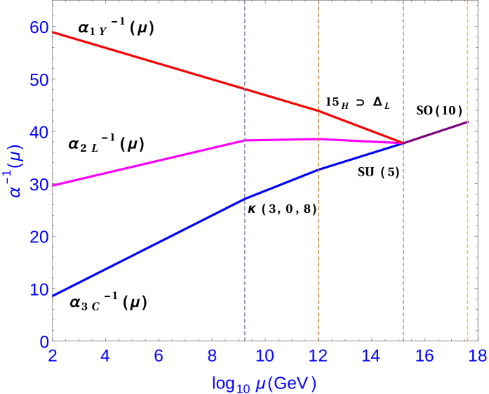
Figure 1: Evolution of gauge couplings with $\kappa(3,0,8)$ at $M_{\kappa}=10^{9.2}$ GeV and all the members of ${15}_{H}$ at $M_{\Delta_{L}}=10^{12}$ GeV shown by the first and the second vertical dashed lines, respectively. The third (fourth) vertical dashed line indicates the SU(5) (SO(10)) unification scale $M_{SU(5)}=10^{15.2}$ GeV ($M_{SO(10)}=10^{17.6}$ GeV).

The predicted mass scales and the GUT fine structure constant in Model-I are

$$M_{\kappa} = 10^{9.2}~{}~{}{\rm GeV},$$

$$M_{\Delta_{L}} = M_{{15}_{H}}=10^{12}~{}~{}{\rm GeV},$$

$$M^{0}_{U} = 10^{15.22}{\rm GeV},$$

$$\alpha_{G}^{-1} = 41.79,$$ (23)

2.3 Model-II: $\eta(3,-1/3,6)$ Assisted Unification with Scalar Singlet DM

In this case of Model-II, the popular and useful representation ${126}_{H}$ that breaks SO(10) and $U(1)_{X}$ with VEV $\langle\Delta_{R}^{0}\rangle=V_{B-L}=M_{SO(10)}\geq 10^{17}$ GeV also leads to matter parity conservation down to low energies. Precision gauge coupling unification of the SM gauge couplings are achieved provided the SM multiplet $\eta(3,-1/3,6)$ originating from the RH scalar triplet $\Delta_{R}(3,1,{\bar{10}})\subset{126}_{H}$ of SO(10) has an intermediate mass $M_{\eta}=10^{10.3}$ GeV. We discuss below how this lighter mass of $\eta$ is derived from SO(10) invariant scalar potential.

2.3.1 Intermediate Mass of $\eta(3,-1/3,6)$

We consider the relevant part of the Higgs potential

$$V_{\kappa} = M_{126}^{2}{126}_{H}^{\dagger}{126}_{H}+m_{126,210}{210}_{H}{126}_{H}^{\dagger}{126}_{H}+\lambda_{(126,210)}{210}_{H}^{2}{126}_{H}^{\dagger}{126}_{H}$$ (24)

$$+ \lambda_{(126)}{126}_{H}^{\dagger}{126}_{H}{126}_{H}^{\dagger}{126}_{H}$$

$$\supset V_{\eta}=\left[M_{126}^{2}+m_{(126,210)}\langle{\bf\Phi}_{(210)}\rangle+\lambda_{(126,210)}\langle{\bf\Phi}_{210}\rangle^{2}+\lambda_{(126)}V_{R}^{2}\right]\eta^{\dagger}{\eta},$$

where the relevant VEVs have been defined in Sec.2.2. Thus, by fine tuning only few of the six quantities $M_{126},m_{(126,210)},\langle{\bf\Phi}_{(210)}\rangle,V_{R},\lambda_{(126)}$ and $\lambda_{(126,210)}$ occurring in eq.(24), it is possible to achieve an intermediate mass for $\eta(3,-1/3,6)$.

We further note that for the first step breaking, SO(10) $\to$ SU(5), ${45}_{H}$ can be also used instead of ${210}_{H}$ in this Model-II. Further the well known SU(5) scalar representation ${24}_{H}$ driving the second step of breaking SU(5) $\to$ SM is also contained in ${45}_{H}$ of SO(10). Then we have the following SM symmetric potential after SU(5) breaking through the VEV $\langle\Phi_{24}\rangle\subset{24}_{H}$ of SU(5)

$$V^{(5)}_{\eta} = \left[M_{50}^{2}+m_{(50,24)}\langle{\bf\Phi}_{(24)}\rangle+\lambda_{(50,24)}\langle{\bf\Phi}_{(24)}\rangle^{2}\right]\eta^{\dagger}{\eta}$$ (25)

$$= M_{\eta}^{2}\eta^{\dagger}{\eta}.$$

Thus fine tuning the relevant parameters in eq.(25) can also lead to the desired intermediate mass of $\eta(3,-1/3,6)$. The RGEs for gauge couplings [68, 69, 70], their solutions including the values of beta function coefficients in different ranges of mass scales are given in Appendix Sec.9.3. When this lone submultiplet $\eta(3,-1/3,6)$ in the grand desert has the intermediate mass, unification of gauge couplings is achieved which has been shown in Fig. 2.

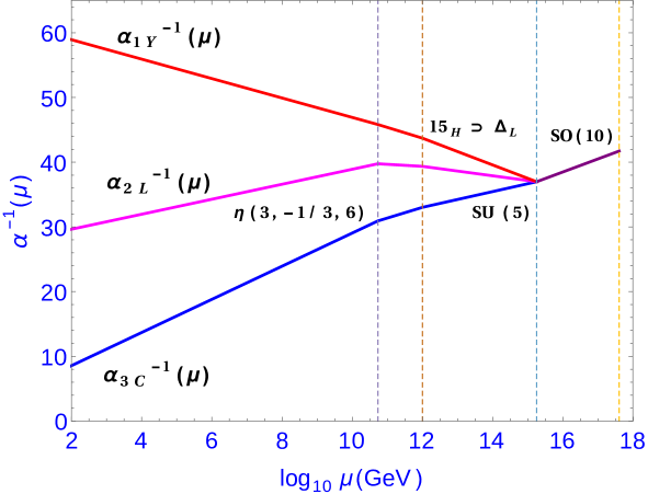
Figure 2: Evolution of gauge couplings with $\eta(3,-1/3,6)$ at $M_{\eta}=10^{10.3}$ GeV and all the members of ${15}_{H}$ at $M_{\Delta_{L}}=10^{12}$ GeV shown by the first and the second vertical dashed lines, respectively. The third (fourth) vertical dashed line indicates the SU(5) (SO(10)) unification scale $M_{SU(5)}=10^{15.2}$ GeV ($M_{SO(10)}=10^{17.6}$ GeV).

The mass scales and the GUT gauge coupling in this case are

$$M_{\eta} = 10^{10.3}~{}~{}{\rm GeV},$$

$$M_{\Delta_{L}} = M_{{15}_{H}}=10^{12}~{}~{}{\rm GeV},$$

$$M^{0}_{U} = 10^{15.3}{\rm GeV},$$

$$\alpha_{G}^{-1} = 38.39,$$ (26)

As in the case of Sec.2.2, all the derivations leading to eq.(15), eq.(17), eq.(18), eq.(20), and eq.(21) are also applicable in this case. Thus a real scalar DM possessing $Z_{MP}=-1$ and originating from ${16}_{H}$ of SO(10) is also predicted in this case.

The requirement of type-II seesaw dominance with precision coupling unification in this model places the common mass of ${15}_{H}$ heavier than $M_{\eta}$ with $M_{\Delta_{L}}=M_{{15}_{H}}\geq 2\times 10^{10}{\rm GeV}$.

2.4 Model-III via Frigerio-Hambye Type Unification [41]

Recently, Frigerio and Hambye [41] have predicted precision coupling unification with fermionic color octet at $\geq 10^{10.3}$ GeV and a 2.7 TeV mass fermionic triplet DM $\Sigma_{F}(3,0,1)$ which may have direct and indirect experimental detection possibilities [41, 71, 72]. The requirement of type-II seesaw dominance as outlined above with precision unification in this model also places the lower bound on the triplet Higgs mass $M_{\Delta_{L}}=M_{{15}_{H}}\geq 10^{10.3}~{}~{}{\rm GeV}$. The resulting evolution of gauge couplings for $M_{\Delta}=M_{{15}_{H}}=10^{12}$ GeV is shown in Fig. 3.

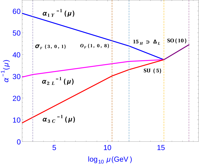
Figure 3: Evolution of gauge couplings through the unification framework [41] with the fermionic DM $\Sigma_{F}(3,0,1)$ at $m_{\Sigma}=10^{3}$ GeV and fermionic color octet at $m_{O_{F}}=10^{10.4}$ GeV indicated by the first and the second vertical dashed lines, respectively. The mass scales for ${15}_{H}$ at $10^{12}$ GeV, SU(5) unification at $M_{SU(5)}=10^{15.26}$ GeV, and SO(10) unification at $M_{SO(10)}=10^{17.6}$ GeV are indicated by the third, fourth, and the fifth vertical dashed lines, respectively.

The mass scales and the GUT coupling in this case are

$$m_{\Sigma} = 10^{3}~{}~{}{\rm GeV},$$

$$m_{O_{F}} = 10^{10.3}~{}~{}{\rm GeV},$$

$$M_{\Delta_{L}} = M_{{15}_{H}}=10^{12}~{}~{}{\rm GeV},$$

$$M^{0}_{U} = M_{U}^{5}=10^{15.26}{\rm GeV},$$

$$\alpha_{G}^{-1} = 33.78.$$ (27)

2.5 Coupling Evolution Above SU(5) Unification Scale

In each of the three different models discussed above we have estimated one-loop evolution for the inverse fine-structure constant using integral form of RG equation,

$$\frac{1}{\alpha_{G}^{(i)}(\mu)}=\frac{1}{\alpha_{G}(M_{U})}-\frac{a^{(i)}_{5}}{2\pi}\ln(\frac{\mu}{M_{U}})\,\,(i=I,II,III)\,$$ (28)

Including the contributions of three standard fermion generations, super heavy gauge bosons (V), scalar(H) and non-standard fermion (F) representations, we have estimated the one-loop value of the SU(5) beta function coefficient $a^{(i)}_{5}(i=I,II,III)$ in each of the three models, Model-I, Model-II, and Model-III .

Model-I:

$${24}_{V},3\times({10}_{F}+{\bar{5}}_{F}),{75}_{H},{15}_{H},{5}_{H}:$$

$$a_{5}^{(I)}=-14/3.\,\,$$ (29)

Model-II:

$${24}_{V},3\times({10}_{F}+{\bar{5}}_{F}),{50}_{H},{24}_{H},{15}_{H},{5}_{H}:$$

$$a_{5}^{(II)}=-11/2.\,\,$$ (30)

Model-III:

$${24}_{V},3\times({10}_{F}+{\bar{5}}_{F}),{24}_{F},{24}_{H},{15}_{H},{5}_{H}:$$ (31)

$$a_{5}^{(III)}=-8.\,\,$$ (32)

These evolutions have been shown by single curves for respective unified gauge couplings for $\mu\geq M_{U}$ in Fig. 1, Fig. 2, and Fig.3 leading to

$$(\frac{1}{\alpha_{G}})_{SO(10)}=40.2,\,40.19\,\,{\rm and}~{}~{}40.45,$$ (33)

for Model-I, Model-II, and Model-III, respectively, at $M_{SO(10)}\simeq 10^{17}$ GeV.

3 Threshold Effects and Proton Lifetime Predictions

3.1 Threshold Corrections on the GUT Scale

Threshold effects due to small log corrections near the GUT scale [73, 74, 75, 76, 77, 78, 70] have been discussed in the Appendix in Sec. 9.3. In order to evaluate these corrections, at first we evaluate the three matching functions $\lambda_{i}(M_{U})(i=1Y,2L,3C)$ representing threshold effects of each model as shown in Sec.2.2.3, Sec.2.3.1, and Sec.2.4

$$\alpha^{-1}_{i}(M_{U})=\alpha^{-1}_{G}-\frac{\lambda_{i}(M_{U})}{12\pi},\,\,(i=1Y,2L,3C).$$ (34)

Analytic expression for threshold effect on the unification scale noted as $\Delta[\ln(M_{U}/M_{Z})]$ in terms of matching functions have been also explicitly derived in Sec.9.3. Estimation of each matching function in terms of small logarithmic correction of different superheavy components needs their beta function coefficients which have been also given in Table 13 and Table 14. Then threshold effects on unification scale have been explicitly derived as shown in detail in Sec.9.3 for Model-I, Model-II and Model-III.

Using partial degeneracy approximation under which all superheavy component masses belonging to the same GUT representation are assumed to be identical [77, 78], threshold effects due to each SU(5) representation and their modification to the GUT scale are presented in Table 1 for Model I, Model-II and Model III. Contributions of different superheavy scalars (S),fermions (F) and gauge bosons (V), are denoted by subscripts S, F, and V respectively. These are from SU(5) representations ${5}_{H},{24}_{H},{75}_{H},{24}_{F}$, and ${24}_{V}$ which have their origins in SO(10) representations ${10}_{H},{45}_{H},{210}_{H},{45}_{F}$ and ${45}_{V}$, respectively. In our notation the small log contribution is proportional to $\eta_{i}=\ln(M_{i}/M^{0}_{U}),(i=5,24,50,75,24_{F},24_{V})$ and $\eta^{\prime}_{X}=\log_{10}(M_{X}/M_{U})(X=S,F,V)$. All the superheavy scalar thresholds proportional to $\eta^{\prime}_{S}=\log_{10}(M_{S}/M_{U}^{0})$ have been derived by maximising their contributions.

Table 1: Predictions of threshold effects on the SU(5) unification scales in Model-I, Model-II and Model-III defined in the text.

	Model-I	Model-II	Model-III
$M_{U}^{0}$(GeV)	$10^{15.244}$	$10^{15.280}$	$10^{15.310}$
$\Delta\ln\left({M_{U}\over M_{Z}}\right)$	$=-0.0196078\eta_{5}$	$=-0.02024\eta_{5}$	$=-0.011\eta_{5}$
	$+0.044563\eta_{75}$	$-0.0445\eta_{24}$	$-0.0549\eta_{24}$
	$+0.9358\eta_{V}$	$-0.31255\eta_{50}$	$-0.1318\eta_{24_{F}}$
		$+0.9382\eta_{V}$	$+1.1538\eta_{V}$
$M_{U}$(GeV)	$10^{15.244\pm 0.11}\times$	$10^{15.28\pm 0.133}\times$	$10^{15.31\pm 0.03}\times$
	$10^{\pm 0.0642\eta^{\prime}_{S}\pm 0.9358\eta^{\prime}_{V}}$	$10^{\pm 0.3773\eta^{\prime}_{S}\pm 0.9352\eta^{\prime}_{V}}$	$10^{\pm 0.0659\eta^{\prime}_{S}\pm 0.13186\eta^{\prime}_{F}\pm 1.1538\eta^{\prime}_{V}}$
$\alpha_{G}^{-1}$	$41.77$	$38.39$	$33.78$

3.2 Proton Lifetime Predictions

Currently, experimentally measured lower limits on the proton life time for the decay modes $p\to e^{+}\pi^{0}$ and $p\to\mu^{+}\pi^{0})$ are[58]

$$\tau_{p}^{expt.}(p\to e^{+}\pi^{0})~{}\geq~{}1.67\times 10^{34}~{}~{}{\rm yrs},$$

$$\tau_{p}^{expt.}(p\to\mu^{+}\pi^{0})~{}\geq~{}7.7\times 10^{33}~{}~{}{\rm yrs}.$$ (35)

Including strong and electroweak renormalization effects on the ${\rm d}=6$ operator and taking into account quark mixing, chiral symmetry breaking effects, and lattice gauge theory estimations, the decay rates are [79, 80, 81],

$$\Gamma(p\rightarrow e^{+}\pi^{0})=(\frac{m_{p}}{64\pi f_{\pi}^{2}}\frac{{g_{G}}^{4}}{{M_{X^{0}}}^{4}})|A_{L}|^{2}|\bar{\alpha_{H}}|^{2}(1+D^{\prime}+F)^{2}\times R,$$ (36)

where $R=[A_{SR}^{2}+A_{SL}^{2}(1+|{V_{ud}}|^{2})^{2}]$ for $SU(5)$, $V_{ud}=0.974=$ the $(1,1)$ element of $V_{CKM}$ for quark mixings, and $A_{SL}(A_{SR})$ is the short-distance renormalization factor in the left (right) sectors. In eq.(36) $A_{L}=1.25=$ long distance renormalization factor. But the short distance renormalisation factor $A_{SL}\simeq A_{SR}$ has been estimated for each model in the Appendix. These are estimated by evolving the ${\rm dim.}6$ operator for proton decay by using the anomalous dimensions [79, 80, 81, 82, 83, 84] and the beta function coefficients for gauge couplings of each model. In eq.(36) $\bar{\alpha}_{H}=$ hadronic matrix elements, $m_{p}=$proton mass $=938.3$ MeV, $f_{\pi}=$ pion decay constant $=139$ MeV, and the chiral Lagrangian parameters are $D=0.81$ and $F=0.47$. Here $\alpha_{H}={\bar{\alpha_{H}}}(1+D^{\prime}+F)$ which has been estimated from lattice gauge theory computations [85, 86]. We have used the hadronic matrix element [86]

$$\frac{{\bar{\alpha}}_{H}(1+D^{\prime}+F)}{{\sqrt{2}}f_{\pi}}=\langle\pi^{0}|(ud)_{R}u_{L}|p\rangle=-0.103(23)(34)\,\,{\rm GeV^{2}},$$ (37)

where the first (second) uncertainty is statistical (systematic). We have estimated values of $A_{SR}$ for different models in Sec.9.4 of Appendix. The corresponding numerical values are given in Table 15. In both the eq.(36) and eq.(38) $M_{X^{0}}$ stands for the degenerate mass of superheavy $X^{\pm 4/3}$ and $Y^{\pm 1/3}$ gauge bosons mediating proton decay. Then the expression for the inverse decay rate or proton lifetime is

$$\Gamma^{-1}(p\rightarrow e^{+}\pi^{0})=\frac{4}{\pi}\frac{f_{\pi}^{2}}{m_{p}}\frac{M_{X^{0}}^{4}}{\alpha_{G}^{2}}\frac{1}{\alpha_{H}^{2}A_{R}^{2}}\frac{1}{F_{q}},$$ (38)

where the GUT-fine structure constant $\alpha_{G}=0.0263$ and the factor $F_{q}=(1+(1+|V_{ud}|^{2})^{2})\simeq 4.8$. This formula has the same form as given in [81] which has been modified here for the SU(5) case.
Using the analytic formula of eq.(38) and the threshold corrected GUT scales presented in Table 1 we now present proton lifetime predictions analytically for the three models using $M_{X^{0}}=M_{U}$ for which threshold effects have been given Table 1.

Model I

$$\tau_{P}\simeq 10^{33.24\pm 0.44\pm 0.256\eta^{\prime}_{S}\pm 3.743\eta^{\prime}_{V}}~{}~{}{\rm yrs},$$ (39)

Model II

$$\tau_{p}\simeq 10^{33.11\pm 0.5335\pm 1.51\eta^{\prime}_{S}\pm 3.74\eta^{\prime}_{V}}~{}~{}{\rm yrs},$$ (40)

Model III

$$\tau_{p}\simeq 10^{33.42\pm 0.120\pm 0.2636\eta^{\prime}_{S}\pm 0.5272\eta^{\prime}_{F}\pm 4.610\eta^{\prime}_{V}}~{}~{}{\rm yrs},$$ (41)

where $\eta^{\prime}_{X}=\log_{10}(M_{X}/M_{U})(X=S,F,V)$. Despite the superheavy gauge boson contributions being from the same SM multiplets $(2,5/3,3)_{V}\oplus(2,-5/3,{\bar{3}})_{V}\subset{24}_{V}\subset SU(5)$ in all the three models, their threshold corrections to proton lifetime are significantly different because of differing renormalization group effects in Model I, Model II and Model III.

Numerical estimations on proton lifetime for Model-I are shown in Table 2 for different splitting factors of superheavy masses. In all the three models, when threshold and coupling constant uncertainties are absent, the predicted $\tau_{P}$ corresponds to the minimum value of the hadronic matrix element in eq.(37) [86].

Table 2: Numerical upper limits on predicted proton lifetime in Model-I as a function of superheavy scalar (S) and gauge boson (V) mass splittings as defined in the text and Appendix. The factor $10^{\pm 0.44}$ is due to uncertainty in input parameters of eq.(155).

${M_{S}\over M_{U}}$	${M_{V}\over M_{U}}$	$\tau_{P}(yrs)$	${M_{S}\over M_{U}}$	${M_{V}\over M_{U}}$	$\tau_{P}(yrs)$
$10$	$2$	$4.19\times 10^{34\pm 0.44}$	$3$	$2$	$3.08\times 10^{34\pm 0.44}$
$1$	$2$	$2.32\times 10^{34\pm 0.44}$	$1$	$3$	$1.06\times 10^{35\pm 0.44}$

Numerical values of proton lifetime predictions for Model-II for different superheavy masses are presented in Table 3.

Table 3: Numerical upper limits on predicted proton lifetime in Model-II as a function of superheavy scalar (S) and gauge boson (V) mass splittings defined in the text and Appendix. The factor $10^{\pm 0.53}$ is due to uncertainty in input parameters of eq.(155).

${M_{S}\over M_{U}}$	${M_{V}\over M_{U}}$	$\tau_{P}(yrs)$	${M_{S}\over M_{U}}$	${M_{V}\over M_{U}}$	$\tau_{P}(yrs)$
$10$	$2$	$4.1\times 10^{34\pm 0.53}$	$1$	$4$	$2.29\times 10^{35\pm 0.53}$
$1$	$3$	$7.84\times 10^{34\pm 0.53}$	$4$	$3$	$1.32\times 10^{35\pm 0.53}$

For the type-II seesaw induced Model-III numerical values of proton lifetime predictions are presented in Table 4 excluding superheavy fermion effects, and in Table 5 including these fermion effects.

Table 4: Numerical upper limits on predicted proton lifetime in Model-III as a function of superheavy scalar (S) and gauge boson(V) mass splittings as defined in the text and assuming superheavy fermions at unification scale. The factor $10^{\pm 0.12}$ is due to uncertainty in input parameters of eq.(155).

${M_{S}\over M_{U}}$	${M_{V}\over M_{U}}$	$\tau_{P}(yrs)$	${M_{S}\over M_{U}}$	${M_{V}\over M_{U}}$	$\tau_{P}(yrs)$
$10$	$2$	$1.17\times 10^{35\pm 0.12}$	$1$	$3$	$4.16\times 10^{35\pm 0.12}$
$3$	$2$	$8.57\times 10^{34\pm 0.12}$	$3$	$3$	$5.55\times 10^{35\pm 0.12}$
$1$	$2$	$6.42\times 10^{34\pm 0.12}$	$2$	$2$	$7.7\times 10^{34\pm 0.12}$

Table 5: Numerical upper limits on predicted proton lifetime in Model-III as a function of superheavy fermion (F) and gauge boson(V) mass splittings as defined in the text assuming superheavy scalars at unification scale. The factor $10^{\pm 0.12}$ is due to uncertainty in input parameters of eq.(155).

${M_{F}\over M_{U}}$	${M_{V}\over M_{U}}$	$\tau_{P}(yrs)$	${M_{F}\over M_{U}}$	${M_{V}\over M_{U}}$	$\tau_{P}(yrs)$
$10$	$2$	$2.16\times 10^{35\pm 0.12}$	$2$	$2$	$9.25\times 10^{35\pm 0.12}$
$6$	$2$	$1.65\times 10^{35\pm 0.12}$	$1$	$2$	$6.42\times 10^{34\pm 0.12}$
$3$	$2$	$1.14\times 10^{35\pm 0.12}$	$25$	$1$	$1.43\times 10^{34\pm 0.12}$

On proton lifetime predictions the following distinguishing features are noted: Although the uncertainty due to input parameters is lowest , the threshold uncertainty due to superheavy gauge bosons ($X^{\pm 4/3},Y^{\pm 1/3}$) is nearly one order larger in Model-III that uses Frigerio-Hambye unification framework [41]. It is quite interesting to note that for natural values of these superheavy gauge boson masses only few times heavier or lighter than the respective GUT scales, the predicted proton lifetimes for $p\to e^{+}\pi^{0}$ are accessible to ongoing searches at Super-Kamiokande and Hyper-Kamiokande [58, 59].

4 Type-II Seesaw Fit to Neutrino Oscillation Data

A hall mark of type-II seesaw dominance is its capability to fit neutrino oscillation data with high precision for all values of mixings and phases.

4.1 Type-II Seesaw Dominance in SO(10) from General Seesaw

Suppressing generation indices, the SO(10) invariant Yukawa Lagrangian

$${\cal L}_{yuk}=Y{16}_{F}{16}_{F}{126}_{H}^{\dagger}+\lambda{16}_{F}{16}_{F}{10}_{H},$$ (42)

predicts the same Majorana Yukawa coupling Y of LH scalar triplet $\Delta_{L}$ to LH dileptons and the RH triplet scalar $\Delta_{R}$ to RHNs. This is due to the fact that both the LH and the RH scalar triplets are contained in ${126}_{H}$. After SO(10) breaking accompanied by $U(1)_{X}$ breaking by $\langle\Delta_{R}\rangle=V_{B-L}\geq 10^{17}$ GeV, the heavy RHN mass matrix is predicted

$$M_{N}=YV_{B-L}.$$ (43)

Below the SU(5) breaking scale, we have SM gauge theory with three additional heavy right-handed neutrinos (RHNs) $N_{i},(i=1,2,3)$ and a heavy Higgs scalar triplet $\Delta_{L}(3,-1,1)\subset{15}_{H}$. The Yukawa Lagrangian encoding type-I+type-II seesaw can be presented as

$$\mathcal{L}=\mathcal{L}^{(I)}+\mathcal{L}^{(II)}$$ (44)

where $\mathcal{L}^{(I)}$ and $\mathcal{L}^{(II)}$ are the additional terms arising due to right handed neutrinos and scalar triplet, respectively. Specifically they are given by

$$-\mathcal{L}^{(I)}=\overline{N_{i}}\lambda_{ij}\tilde{\phi}^{\dagger}l_{L_{j}}+\frac{1}{2}\overline{N_{i}}Y_{ij}C\overline{N_{j}}^{T}V_{B-L}+h.c~{}~{},$$ (45)

$$-\mathcal{L}^{(II)}=l_{L_{i}}^{T}Ci\tau_{2}Y_{ij}(\frac{\vec{\tau}.\vec{\Delta_{L}}}{\sqrt{2}})l_{L_{j}}+M_{\Delta}^{2}Tr[\Delta_{L}^{\dagger}\Delta_{L}]+\mu_{\Delta}\tilde{\phi}^{\dagger}(\frac{\vec{\tau}.\vec{\Delta_{L}}}{\sqrt{2}})^{\dagger}\phi+h.c,$$ (46)

where $l_{L_{i}}^{T}=(\nu_{L_{i}},~{}e_{L_{i}})$ ($i$ is the lepton generation index) and the standard Higgs doublet components $\phi^{T}=(\phi^{+},\phi^{0})\subset{10}_{H}$ of SO(10). Here $\tilde{\phi}=i\tau_{2}\phi^{\ast}$, $\vec{\tau}=(\tau_{1},\tau_{2},\tau_{3})$ ($\tau_{i}$ are the $2\times 2$ Pauli spin matrices). Similarly the scalar triplet $\Delta_{L}$ in the adjoint representation of $SU(2)_{L}$ is expressed as $\vec{\Delta_{L}}=(\Delta_{L}^{1},\Delta_{L}^{2},\Delta_{L}^{3})$. The Yukawa couplings $Y$ and $\lambda$ are both $3\times 3$ matrices in flavour space and $C$ is the charge conjugation matrix. Thus the term $(\frac{\vec{\tau}.\vec{\Delta_{L}}}{\sqrt{2}})$ can be written explicitly as

$$(\frac{\vec{\tau}.\vec{\Delta_{L}}}{\sqrt{2}})=\left(\begin{array}[]{cc}\frac{\Delta^{+}}{\sqrt{2}}&\Delta^{++}\\ \Delta^{0}&-\frac{\Delta^{+}}{\sqrt{2}}\\ \end{array}\right)_{L}$$ (47)

where $\Delta_{L}^{0}=\frac{1}{\sqrt{2}}(\Delta_{L}^{1}+i\Delta_{L}^{2}),~{}~{}\Delta_{L}^{+}=\Delta_{L}^{3},~{}~{}\Delta_{L}^{++}=\frac{1}{\sqrt{2}}(\Delta_{L}^{1}-i\Delta_{L}^{2})$. Compared to SM extended theory with added $\Delta_{L}$+RHNs [50, 53], these Lagrangians have the following distinctions. The RHN mass of SO(10) breaking origin $M_{N}=YV_{B-L}$ appearing in the second term of eq.(45) has the same Majorana coupling matrix $Y$ that also defines the type-II seesaw term $m_{\nu}^{II}$ of eq.(56) originating from first term of eq.(46). As a result, the freedom of choosing a RHN diagonal basis [50, 53] is lost these SO(10) models. On the other hand the same unitary PMNS matrix $U$ that diagonalises neutrino mass matrix under type-II dominance approximation also diagonalises $M_{N}$. This has been shown below to lead to an inevitable transformation on the Dirac neutrino Yukawa coupling $\lambda\to\lambda U^{\ast}$ and, therefore, to new class of CP-asymmetry formulas for leptogenesis. Another important difference from SM extension is that the Dirac neutrino Yukawa coupling matrix $\lambda$ is predicted to be known from SO(10) symmetry. Further in the SM extension the trilinear coupling $\mu_{\Delta}$ in the third term of eq.(46) is a lepton number conserving bare mass term. On the other hand in these SO(10) breaking models, the $U(1)_{X}$ breaking VEV predicts $\mu_{\Delta}$ as the product of a quartic coupling and $V_{B-L}$

$$V_{(126,10)} = \lambda_{(126,10)}{126}_{H}^{\dagger}{126}_{H}{10}_{H}{10}_{H}\supset\mu_{\Delta}\Delta_{L}\phi\phi+h.c.,$$

$$\mu_{\Delta} = \lambda_{(126,10)}V_{B-L}.$$ (48)

As shown below in Fig.4, this interaction is responsible for the second vertex generating type-II seesaw contribution.

For the type-II seesaw mass term the Feynman diagram is shown in Fig.4.

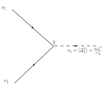
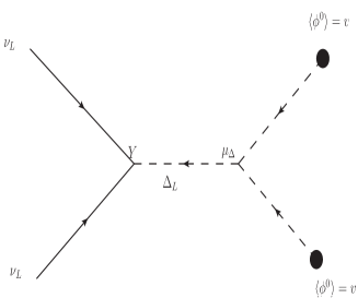
Figure 4: Schematic representation of generation of Type-II seesaw term comprised of first and third terms of eq.(46)(left panel). The same quantity after $\Delta_{L}$ gets induced VEV in the SM extension (right panel).

The SO(10) predicted interaction potential of eq.(48) in conjunction with $Y\Delta_{L}l^{c}l^{c}$ Yukawa term leads to the induced vacuum expectation value of $\Delta_{L}$ whenever the SM doublet $\phi\subset{10}_{H}$ acquires electroweak VEV $v=246$ GeV,

$$v_{L}=\frac{\mu_{\Delta}v^{2}}{2M_{\Delta}^{2}},$$ (49)

leading to the type-II seesaw formula

$$m_{\nu}^{II}=Yv_{L}.$$ (50)

In the SO(10) case $\mu_{\Delta}=\lambda_{(126,10)}V_{B-L}$ which originates from the scalar interaction term $\lambda_{(126,10)}{126}_{\rm H}^{\dagger}{126}_{H}{10}_{H}{10}_{H}$ and the generalised expression for the induced VEV is

$$v_{L}=\frac{\lambda_{(126,10)}V_{B-L}v^{2}}{2M_{\Delta}^{2}}.$$ (51)

However when the self energy correction to the triplet mass is taken as $\lambda_{(126,10)}V_{B-L}\simeq M_{\Delta}$ leading to a simpler form of the induced VEV

$$v_{L}=\frac{v^{2}}{2M_{\Delta}^{2}}.$$ (52)

Thus the general form of seesaw formula predicted by SO(10) is

$$m_{\nu} = m_{\nu}^{II}+m_{\nu}^{I}=Yv_{L}-M_{D}^{T}M_{N}^{-1}M_{D}$$ (53)

$$= Y\mu_{\Delta}v^{2}/{(2M_{\Delta}^{2})}-\frac{v^{2}}{2V_{B-L}}\lambda\frac{1}{Y}\lambda^{T}.$$

It is crucial to note that the same Majorana coupling matrix $Y$ occurs in the type-II as well as type-I seesaw term which is a general prediction of any SO(10) with Higgs representations ${126}_{H}$ and ${10}_{H}$.

In comparison the general seesaw formula resulting from SM extension with $\Delta_{L}$+RHNs is [53]

$$m_{\nu} = {\cal M}_{\Delta}^{\nu}+{\cal M}_{N}^{\nu}=Yv_{L}-M_{D}^{T}M_{N}^{-1}M_{D}$$ (54)

$$= Y\mu_{\Delta}v^{2}/{(2M_{\Delta}^{2})}-\frac{v^{2}}{2}\lambda\frac{1}{M_{N}}\lambda^{T}$$

where the Majorana coupling $Y$ occurs only in the type-II seesaw term. Thus, in general, the active neutrino mass matrix consists of both Type-I and Type-II seesaw terms. Depending upon the magnitude of the two terms, both the contributions are included as in the case of hybrid seesaw [32, 46]. In the specifically designed SO(10) breakings, the models allow Type-II seesaw dominance [61, 62]. It is clear from eq.(53) that type-II seesaw dominance occurs when

$$M_{\Delta}\ll M_{N},\,\,{\rm or}\,\,M_{\Delta}\ll V_{B-L}$$ (55)

In the three models discussed in Sec.2, theoretically allowed values of $M_{\Delta}$ consistent with precision gauge coupling unification are $M_{\Delta}=10^{9.3}-10^{15}$ GeV in Model-I and $M_{\Delta}=10^{10.3}-10^{15}$ GeV in both Model-II and Model-III whereas in all the three models $V_{B-L}\geq 10^{17}$ GeV. Thus the condition of type-II seesaw dominance is satisfied to an excellent approximation. We, therefore, use the type-II dominance approximation

$$m_{\nu}=m_{\nu}^{II}=Yv_{L},$$ (56)

where $v_{L}$ is given in eq.(49), to parametrise neutrino data as discussed in the next Sec.4.2.

4.2 Neutrino Mass Matrix from Oscillation Data

Using standard parametrisation of PMNS matrix $U_{PMNS}(\equiv U)$ [87], the $3\times 3$ neutrino mass matrix is represented as

$$m_{\nu}=U_{PMNS}~{}diag(m_{1},m_{2},m_{3})U_{PMNS}^{T}$$ (57)

where $m_{i}(i=1,2,3)=$ mass eigen values and using the PDG convention [87]

$$U_{\rm{PMNS}}=\left(\begin{array}[]{ccc}c_{12}c_{13}&s_{12}c_{13}&s_{13}e^{-i\delta}\cr-s_{12}c_{23}-c_{12}s_{23}s_{13}e^{i\delta}&c_{12}c_{23}-s_{12}s_{23}s_{13}e^{i\delta}&s_{23}c_{13}\cr s_{12}s_{23}-c_{12}c_{23}s_{13}e^{i\delta}&-c_{12}s_{23}-s_{12}c_{23}s_{13}e^{i\delta}&c_{23}c_{13}\cr\end{array}\right)diag(e^{\frac{i\alpha_{M}}{2}},e^{\frac{i\beta_{M}}{2}},1)$$ (58)

where $s_{ij}=\sin\theta_{ij},c_{ij}=\cos\theta_{ij}$ with $(i,j=1,2,3)$, $\delta$ is the Dirac CP phase and $(\alpha_{M},\beta_{M})$ are Majorana phases. During our actual calculation the mass eigenvalues and mixing angles are taken to be the best fit values of the present oscillation data[3, 4]presented in Table 6 below.

Table 6: Input data from neutrino oscillation experiments [3, 4]

Quantity	best fit values	$3\sigma$ ranges
$\Delta m_{21}^{2}~{}[10^{-5}eV^{2}]$	$7.39$	$6.79-8.01$
$|\Delta m_{31}^{2}|~{}[10^{-3}eV^{2}](NO)$	$2.52$	$2.427-2.625$
$|\Delta m_{32}^{2}|~{}[10^{-3}eV^{2}](IO)$	$2.51$	$2.412-2.611$
$\theta_{12}/^{\circ}$	$33.82$	$31.61-36.27$
$\theta_{23}/^{\circ}(NO)$	$49.6$	$40.3-52.4$
$\theta_{23}/^{\circ}(IO)$	$49.8$	$40.6-52.5$
$\theta_{13}/^{\circ}(NO)$	$8.61$	$8.22-8.99$
$\theta_{13}/^{\circ}(IO)$	$8.65$	$8.27-9.03$
$\delta/^{\circ}(NO)$	$215$	$125-392$
$\delta/^{\circ}(IO)$	$284$	$196-360$

We now determine the $m_{\nu}$ matrix for the normally ordered (NO) masses. For the sake of convenience we take the mass of the lightest neutrino as $m_{1}=0.001$ eV. Then using the solar and atmospheric mass squared differences for NO from Table 6, the other two neutrino mass eigenvalues are computed with $m_{2}=0.00865$ eV and $m_{3}=0.0502$ eV. Using these mass eigenvalues and the best fit values of the mixing angles and Dirac CP phases, eq.(57) gives

$$m_{\nu}^{NO}(\rm eV)=\left(\begin{array}[]{ccc}0.00367-0.00105i&-0.00205+0.00346i&-0.00634+0.00294i\cr-0.00205+0.00346i&0.03154+0.00034i&0.02106-0.0001i\cr-0.00634+0.00294i&0.02106-0.0001i&0.02383-0.00027i\cr\end{array}\right)~{}~{}.$$ (59)

Keeping all the other parameters at their best fit values, we derive the numerical structure of $m_{\nu}$ for another value of the Dirac CP phase $\delta=170^{\circ}$ (which is within the given $3\sigma$ range)

$$m_{\nu}^{NO}(\rm eV)=\left(\begin{array}[]{ccc}0.00435-0.00038i&-0.00293-0.00104i&-0.00708-0.00089i\cr-0.00293-0.00104i&0.03165-0.00010i&0.02107+1.95\times 10^{-6}i\cr-0.00708-0.00089i&0.02107+1.95\times 10^{-6}i&0.02377+0.00007i\cr\end{array}\right)~{}~{}.$$ (60)

For inverted ordering (IO), setting the lightest mass eigenvalue $m_{3}=0.001$ eV and using the mass squared differences from Table 6, we get $m_{1}=0.04938$ eV, $m_{2}=0.0501$ eV. Then the value of $m_{\nu}$ corresponding to best fit values of parameters turns out to be

$$m_{\nu}^{IO}(\rm eV)=\left(\begin{array}[]{ccc}0.0484-0.00001i&-0.001122+0.0055i&-0.00137+0.00471i\cr-0.001122+0.0055i&0.02075-0.00025i&-0.02459-0.00026i\cr-0.00137+0.00471i&-0.02459-0.00026i&0.02910-0.00026i\cr\end{array}\right).$$ (61)

Similarly the structure of the mass matrix for another value of $\delta=200^{\circ}$, which is in a different quadrant, is estimated

$$m_{\nu}^{IO}(\delta=200^{\circ})(\rm eV)=\left(\begin{array}[]{ccc}0.04849-0.00001i&0.005399+0.00196i&0.00413+0.00166i\cr 0.005399+0.00196i&0.02189+0.00043i&-0.02369+0.000352i\cr 0.00413+0.00166i&-0.02369+0.000352i&0.029816+0.000285i\cr\end{array}\right).~{}~{}$$ (62)

Using the up-quark diagonal basis the Dirac neutrino mass matrix is taken to be nearly equal to the up quark mass matrix[46]

$$M_{D}(\rm GeV)\simeq{\rm diag}(.00054,.26302,81.99).$$ (63)

from which the coupling matrix is $\lambda\simeq\frac{M_{D}}{v/\sqrt{2}}$.

The masses of the heavy neutrinos are generated at very high $SO(10)$ breaking scale which also induces the trilinear coupling $\mu_{\Delta}$ as noted above

$$M_{N} = YV_{B-L},$$

$$\mu_{\Delta} = \lambda_{(126,10)}V_{B-L},$$ (64)

where $V_{B-L}=\langle\Delta_{R}^{0}\rangle\geq 10^{17}$ GeV and $\lambda_{126,10}{126}_{H}{126}_{H}^{\dagger}{10}_{H}{10}_{H}$ is the SO(10) invariant scalar interaction term. Using eq.(43) and eq.(56) we have

$$M_{N} = m_{\nu}\frac{V_{B-L}}{v_{L}}$$

$${\hat{M}}_{N} = diag(m_{1},m_{2},m_{3})\frac{V_{B-L}}{v_{L}},$$ (65)

which predicts the relation in eq.(2). Among all the variables in the RHS of eq.(65), only the numerical value of $v_{L}$ is unknown. Again $v_{L}$ itself contains two unknowns $\mu_{\Delta}$ and $M_{\Delta}$ which are varied in suitable ranges to generate a parameter space where we implement leptogenesis in Sec.7.

5 Scalar Dark Matter Prediction with Vacuum Stability

In this section we show how WIMP (weakly interacting massive particles) DM and vacuum stability [60] issues are reconciled in Model-I and Model-II using our derivation discussed in Sec. 2.2.2. In Sec.6 we also discuss two different ways for confronting the vacuum stability issue in Model-III.

5.1 Intrinsic Dark Matter from SO(10)

The scalar dark matter candidate that we utilise here can be identified with the imaginary part of the SM singlet component of ${16}_{H}\subset$ SO(10) which carries odd matter parity [39, 40, 41]

$$\xi\equiv\chi_{S}^{I}=Im(\chi_{S})\subset{16}_{H}\subset{\rm SO(10)}.$$ (66)

In Sec.2.2.2 we have shown how this imaginary part of the real scalar singlet carrying odd matter parity can be as light as desired while keeping the real part at the GUT scale, or vice versa.

It is well known that the standard model Higgs potential

$$V_{SM}=-{\mu}^{2}\phi^{\dagger}\phi+\lambda_{\phi}(\phi^{\dagger}\phi)^{2},$$ (67)

develops instability as the Higgs quartic coupling $\lambda_{\phi}$ runs negative at an energy scale $10^{9}-10^{10}$ GeV. In the last step of our symmetry breaking chain of eq.(9), the SM gauge symmetry is broken spontaneously to $U(1)_{em}\times SU(3)_{C}$ by the electroweak VEV of the standard Higgs doublet $\phi\subset{5}_{H}\subset$ SU(5). As a result, only the SM Higgs $\phi$ remains light at the electroweak scale while the color triplet in ${5}_{H}$ acquires mass at the SU(5) scale [88, 89]. But, as shown in Sec.2.2.2, the matter parity odd real scalar singlet $\xi$ could be as light as $\sim(100-1000)$ GeV in each of the three models leading to the modified scalar potential

$$V=-\mu^{2}\phi^{\dagger}\phi+\mu_{\xi}^{2}\xi^{\dagger}\xi+\lambda_{\phi}(\phi^{\dagger}\phi)^{2}+\lambda_{\xi}(\xi^{\dagger}\xi)^{2}+2\lambda_{\phi\xi}(\phi^{\dagger}\phi)(\xi^{\dagger}\xi).$$ (68)

In eq.(68) $\lambda_{\xi}\simeq\lambda_{16}\equiv$ dark matter self-coupling associated with the interaction $\lambda_{16}[{16}_{H}^{\dagger}{16}_{H}]^{2}$ and $\lambda_{\phi\xi}\simeq\lambda_{10,16}$ which is associated with $\lambda_{10,16}{16}_{H}^{\dagger}{16}_{H}{10}_{H}^{2}$. This latter type SO(10) invariant interaction has induced the $\phi-\xi$ Higgs portal interaction of the SM effective gauge theory. Also $\mu_{\xi}^{2}\equiv M_{\rm Im}^{2}$ as defined through eq.(20) of Sec. 2.2.2. The VEV of the standard Higgs doublet redefines the DM mass parameter

$$M_{DM}^{2}=2(\mu_{\xi}^{2}+\lambda_{\phi\xi}^{2}v^{2}),$$

$$m_{\phi}^{2}=2\mu^{2}=2\lambda_{\phi}v^{2}.$$ (69)

In SM extensions [90, 91, 92, 93] the origins of the scalar DM, its mass, and the DM stabilising discrete symmetry are unknown apriori. On the other hand, in this work, all these quantities including the SM Higgs are intrinsic to self sufficient SO(10) theory. In order to constrain the Higgs portal coupling $\lambda_{\phi\xi}$ we use recent results of DM direct detection experiments like LUX-2016[94], XENON1T[95, 96], PANDA-X-II[97]. Bounds on DM relic density $(\Omega_{\rm DM}h^{2}=0.1172-0.1224)$ as reported by WMAP[98] and Planck[6] are also taken into account. We first proceed to calculate the relic density for different combinations of dark matter mass $(m_{\xi})$ and the Higgs portal coupling $(\lambda_{\phi\xi})$. It is then easy to restrict the values of $m_{\xi}$ and $\lambda_{\phi\xi}$ using the bound on relic density as quoted above. In direct detection experiments it is assumed that WIMPs passing through earth scatter elastically off the target material of the detector. The energy transfer to the detector nuclei can be measured through various types of signals. All those direct detection experiments provide DM mass vs DM-nucleon scattering cross section plot which clearly separates two regions: allowed (regions below the curve) and forbidden (regions above the curve). Our aim is to constrain the model parameters $(\lambda_{\phi\xi},m_{\xi})$ using bounds on relic density as well as exclusion plots from several DM direct detection experiments.

5.1.1 Estimation of Relic Density:

Defining $\Gamma$ (H) as the particle decay rate (Hubble parameter), at a certain stage of evolution of the Universe a particle species is said to be coupled if $\Gamma>H$ or decoupled if $\Gamma<H$. The WIMP DM particle has been decoupled from the thermal bath at some early epoch and has remained as a thermal relic.

In order to calculate the relic density of the scalar singlet DM, we solve the Boltzmann equation[99, 100] for the corresponding particle species which is given by

$$\frac{dn}{dt}+3Hn=-\langle\sigma v\rangle(n^{2}-n_{eq}^{2})$$ (70)

where $n=$ actual number density at a certain instant of time and $n_{eq}=$ equilibrium number density of scalar DM. Here $v=$ velocity and $\langle\sigma v\rangle=$ thermally averaged annihilation crosssection. Approximate solution of Boltzmann equation gives the expression of relic density[100, 101, 102]

$$\Omega_{\rm DM}h^{2}=\frac{1.07\times 10^{9}x_{F}}{\sqrt{g_{\ast}}M_{pl}\langle\sigma v\rangle}$$ (71)

where $x_{F}=m_{\xi}/T_{F}$, $T_{F}=$ freezeout temperature, $g_{\ast}=$ effective number of massless degrees of freedom and $M_{pl}=1.22\times 10^{19}$ GeV. $x_{F}$ can be computed by iteratively solving the equation

$$x_{F}=\ln\left(\frac{m_{\xi}}{2\pi^{3}}\sqrt{\frac{45M_{pl}^{2}}{8g_{\ast}x_{F}}}\langle\sigma v\rangle\right).$$ (72)

In eq.(71) and eq.(72), the only particle physics input is the thermally averaged annihilation cross section. The total annihilation cross section is obtained by summing over all the annihilation channels of the singlet DM which are $\xi\xi\rightarrow f\bar{f},W^{+}W^{-},ZZ,hh$ where $f$ is symbolically used for all the fermions. Using the expression of total annihilation cross section[103, 104, 105, 106] in eq.(72) at first we compute $x_{F}$ which is then plugged into eq.(71) to yield the relic density. Two free parameters involved in this computation are mass of the DM particle $m_{\xi}$ and the Higgs portal coupling $\lambda_{\phi\xi}$. The relic density has been estimated for a wide range of values of the DM matter mass ranging from few GeVs to few TeVs while the coupling $\lambda_{\phi\xi}$ is also varied simultaneously in the range $(10^{-4}-1)$. The parameters $(m_{\xi},\lambda_{\phi\xi})$ are constrained by using the bound on the relic density reported by WMAP and Planck. In Fig.5 we show only those combinations of $\lambda_{\phi\xi}$ and $m_{\xi}$ which are capable of producing relic density in the experimentally observed range.

5.1.2 Bounds from Direct Detection Experiments

We get exclusion plots of DM-nucleon scattering cross section and DM mass from different direct detection experiments. The spin independent scattering cross section of singlet DM on nucleon is given by[107]

$$\sigma^{\rm SI}=\frac{4f^{2}\lambda_{\phi\xi}^{2}\mu^{2}m_{N}^{2}}{\pi m_{\xi}^{2}m_{h}^{4}}~{}~{}({\rm cm}^{2})$$ (73)

where $m_{h}=$ mass of the SM Higgs ($\sim 125$ GeV), $m_{N}=$ nucleon mass $\sim 939$ MeV, $\mu=(m_{\xi}m_{N})/(m_{\xi}+m_{N})=$ reduced DM-nucleon mass and the factor $f\sim 0.3$. Using eq.(73) the exclusion plots of $\sigma-m_{\xi}$ plane can be easily brought to $\lambda_{\phi\xi}-m_{\xi}$ plane. We superimpose the $\lambda_{\phi\xi}-m_{\xi}$ plots for different experiments on the plot of allowed parameter space constrained by relic density bound. So the parameter space $(\lambda_{\phi\xi}~{}vs~{}m_{\xi})$ constrained by both the relic density bound and the direct detection experiments can be obtained from Fig.5.

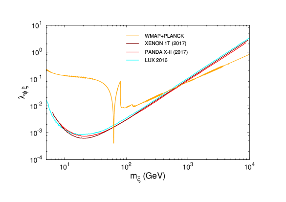
Figure 5: The yellow curve denotes the values of the parameters $(\lambda_{\phi\xi},m_{\xi})$ allowed by the relic density bound $(\Omega_{\rm DM}h^{2}=0.1172-0.1224)$ as observed by Planck and WMAP. The cyan, brown and red curves are exclusion plots obtained from dark matter direct detection experiments LUX-2016, XENON1T(2017) and Panda-XII(2017), respectively. Any point below those plots are allowed by direct detection experiments. It is to be noted that the Panda-XII experiment has provided the most stringent bound till date.

In Fig.5 the points on the yellow curve which are also below the exclusion lines of the direct detection experiments are allowed by both the relic density as well as the upper bounds on the DM-nucleon annihilation cross section as reported by the direct detection experiments. From the Fig.5 it is clear that scalar singlet dark matter with mass below $\sim 750$ GeV is ruled out by direct detection experiments. Although few allowed points can be obtained around $m_{\xi}\sim 62$ GeV, for those points the Higgs portal coupling is very low and the mass of the DM particle is also highly fine tuned.

5.1.3 Resolution of Vacuum Stability

To resolve the vacuum instability problem we choose few points on the yellow curve (allowed by relic density bound) of Fig.5 at high mass region. We examine whether the vacuum has now become stable upto the Planck scale after the addition of the scalar singlet WIMP DM to SM. To trace the evaluation of the SM Higgs quartic coupling upto higher energy scales, we solve the corresponding set of renormalisation group equations eq.(117) which are given in Appendix.9.1. The corresponding values of the Higgs portal coupling $(\lambda_{\phi\xi})$ and self coupling of the scalar singlet DM $(\lambda_{\xi})$ at the electroweak scale which are taken to be the initial value of our analysis are stated in Table.7. Thorough analysis of vacuum stability using those chosen points $(\lambda_{\phi\xi},m_{\xi})$ reveals that it is not possible to cure the vacuum instability problem of SM by adding a scalar singlet WIMP DM of mass below $1.4$ TeV. The evolution of SM Higgs quartic coupling $(\lambda_{\phi})$ with the energy scale $(\mu)$ for two different values of DM masses, $1.5$ and $2$ TeV, is depicted in Fig.6 which clearly indicates that this vacuum instability is indeed resolved for DM mass $1.5$ TeV.

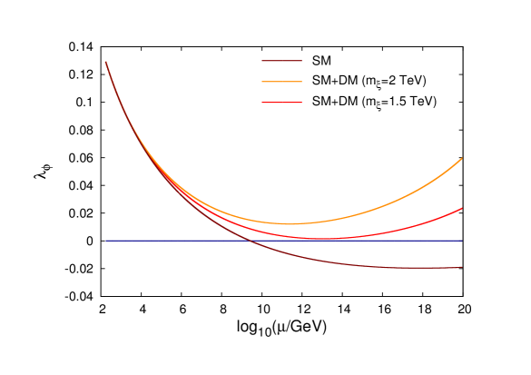
Figure 6: Running of SM Higgs quartic coupling in presence of scalar singlet WIMP dark matter. The yellow and red curves are for dark matter masses $2$ TeV and $1.5$ TeV respectively whereas the brown curve is for standard model alone.

Table 7: Initial values of coupling constants at top quark mass for two different values of the dark matter mass. The values of $\lambda_{\phi\xi}$ and $m_{\xi}$ are obtained from the plot of constrained parameter space of Fig.5.

$m_{\xi}$ ( TeV )	$\lambda_{\phi\xi}(m_{t})$	$\lambda_{\xi}(m_{t})$	$\lambda_{\phi}(m_{t})$	$g_{1Y}(m_{t})$	$g_{2L}(m_{t})$	$g_{3C}(m_{t})$	$y_{t}(m_{t})$
$1.5$	$0.118$	$0.22$
			$0.129$	$0.35$	$0.64$	$1.16$	$0.94$
$2$	$0.158$	$0.1$

6 Vacuum Stability with Triplet Fermionic Dark Matter

We point out below two different ways to resolve the vacuum stability problem of the SM scalar potential existing in the original model [41] or its type-II seesaw dominance induction carried out through the Model-III.

6.1 Intermediate Mass Scalar Singlet Threshold Effect

Even after the implementation of type-II seesaw dominance through Frigerio-Hambye framework, an interesting solution to the vacuum stability problem applies as noted in [60]. In this mechanism a Higgs scalar singlet originating from any one of SO(10) scalar representations like ${45}_{H},{54}_{H},{210}_{H},...$ is made light to have mass around $10^{8}-10^{9}$ GeV. Then vacuum expectation value of this scalar singlet generates threshold effects that prevents the SM Higgs quartic coupling from being negative at higher scales. In this case the triplet fermion DM mass remains at $\sim 2.7$ TeV [41] and needs non-perturbative Sommerfeld enhancement to account for relic density.

6.2 Through the Added Presence of Light Scalar Singlet Dark Matter

6.2.1 Combined Effect on Relic Density

It has been shown [41] that the neutral component of the triplet fermion $\Sigma(3,0,1)$ can play the role of WIMP dark matter and the correct amount of relic abundance is generated when the mass of the triplet is $\sim 2.4$ TeV. This mass value arrived through perturbative calculation is further shifted to $2.7$ TeV when the non perturbative Sommerfeld effect is also taken into account. The triplet fermionic DM model seems to be somewhat constrained from various direct detection experiments. It is found that the DM-nucleon scattering cross section[108] at $m_{\Sigma}\sim 1$ TeV nearly touches the upper bound given in the most recent XENON1T result. Thus, there may be possibility of facing more severe constraint in near future unless the presence of the $\sim 2.7$ TeV triplet fermionic DM is confirmed through precision measurements. In the indirect detection experiment, signals are produced in the annihilation process: DM DM $\rightarrow$ SM particles. Here we have tree level annihilation only to $W^{+}W^{-}$ channel. The annihilation cross section to $W^{+}W^{-}$ shows a peak near $m_{\Sigma}\sim 2.7$ TeV when nonperturbative effects are taken into account. But this high value of annihilation cross section exceeds the upper limit given by the combined analysis [109] of Fermi LAT and MAGIC. So it can be inferred that when the dark matter is composed of only the fermion triplet, it fails to satisfy all the experimental constraints (relic density, direct and indirect detection bounds) simultaneously. In other words the triplet fermionic dark matter appears to be strongly constrained by indirect detection experiments. Even after resolution of the instability through such threshold effect[60] , the $2.7$ TeV mass triplet fermionic DM model may have to face the constraints due to relic density and direct and indirect detection experiments.

Now we modify the Model-III in such a way that all the above mentioned difficulties are evaded without disturbing the gauge coupling unification or type-II seesaw driven leptogenesis. We utilise the real gauge singlet scalar $(\xi\subset 16_{H}^{\dagger},m_{\xi}=500-2000{\rm GeV})$ which acts a WIMP dark matter in the modified scenario. Thus the total relic abundance is now shared by the fermion triplet [41] and the real scalar singlet. Since the dark matter has now two components, the constraint relations from direct and indirect detection experiments will also have a small change.

We keep the mass of the triplet fermionic dark matter at $m_{\Sigma}=1$ TeV. The interesting point about the choice of this triplet mass is that at this lower mass $\sim 1$ TeV, we need not include the non-perturbative Sommerfeld enhancement to match the relic density and the annihilation crosssection to $W^{+}W^{-}$ as a perturbative calculation gives us a fair estimation of the cross section. But the relic abundance produced only due to the triplet DM ($m_{\Sigma}=1$ TeV) is much less than the experimental value quoted by Planck[6] and WMAP[98]. This disagreement is compensated through the intervention of the real singlet DM candidate $\xi$. Since the scalar singlet can not have any renormalisable interaction with the fermionic triplet DM $\Sigma_{F}$, we can estimate the relic density for fermionic triplet ($(\Omega h^{2})_{1}$) and scalar singlet $((\Omega h^{2})_{2})$ separately and add them up to get the total relic density

$$(\Omega h^{2})_{t}=(\Omega h^{2})_{1}+(\Omega h^{2})_{2}~{}.$$ (74)

To estimate the relic abundance of the neutral component $\Sigma^{0}$ that acts as dark matter, we have to take into account the annihilations and co-annihilations of $\Sigma^{0}$ itself and $\Sigma^{+}\Sigma^{-}$. Calculating all such contributions $(\sigma(\Sigma^{0},\Sigma^{0}),\sigma(\Sigma^{0},\Sigma^{\pm})$ $,\sigma(\Sigma^{+},\Sigma^{-}),\sigma(\Sigma^{\pm},\Sigma^{\pm}))$ and adding them up after multiplying by suitable weightage factor[64] we get the effective cross section $\langle\sigma_{eff}|v|\rangle$ which is thereafter plugged into the equation

$$(\Omega h^{2})_{1}=\frac{1.07\times 10^{9}x_{F}}{\sqrt{g_{\ast}}M_{pl}\langle\sigma_{eff}|v|\rangle}$$ (75)

to obtain the relic density due to the triplet fermion DM. It is to be noted that $x_{F}=m_{\Sigma}/T_{F}$ in the above equation is related to the freezeout temperature $T_{F}$ and is determined by the iterative solution of the equation [64]

$$x_{F}=\ln\left[\frac{1}{2\pi^{3}}\sqrt{\frac{45}{2}}\frac{M_{pl}m_{\Sigma}\langle\sigma_{eff}|v|\rangle}{\sqrt{g_{\ast}x_{F}}}\right].$$ (76)

The computational procedure for relic density $(\Omega h^{2})_{2}$ due to scalar singlet has already been discussed in Sec.5.1.1. In the estimation of the total relic density there are three free parameters: mass of the fermion triplet $(m_{\Sigma})$, mass of the scalar singlet $(m_{\xi})$ and the Higgs portal coupling $(\lambda_{\phi\xi})$. The quantity $(\Omega h^{2})_{1}(m_{\Sigma}=1)$ TeV is found to be much less than the experimental value. The other part of the relic density required to meet the experimental constraint $(0.1172<(\Omega h^{2})_{t}<0.1224)$ is generated by the real scalar singlet. It is worthwhile to mention that we have varied $\lambda_{\phi\xi}$ and $m_{\xi}$ over a wide range of values and $(\lambda_{\phi\xi},m_{\xi})$ get their first round of constraint from the relic density bound given above. With the set of values of $(\lambda_{\phi\xi},m_{\xi})$ already restricted by relic density bound, we proceed further to constrain them by direct detection bound. For this two component dark matter, the constraint relation appears as [64, 110]

$$\frac{\epsilon_{\Sigma}}{m_{\Sigma}}\sigma_{\Sigma N}+\frac{\epsilon_{\xi}}{m_{\xi}}\sigma_{\xi N}<\frac{\sigma_{0}}{m_{0}}$$ (77)

where the symbols have the following meanings. $\sigma_{0},m_{0}$ are DM-nucleon scattering cross section and mass of the dark matter, respectively, for single component dark matter scenario. Now for the two component dark matter scenario under consideration $\sigma_{\Sigma N}(\sigma_{\xi N})$ is the scattering cross section of $\Sigma(N)$ with detector nucleon and $m_{\Sigma}(m_{\xi})$ is its mass. The factor $\epsilon_{i}$ designates the fraction of density of the $i$th dark matter particle in a certain model: $\epsilon_{i}=\rho_{i}/\rho_{0}$ which can also be expressed in terms of thermally averaged annihilation cross sections as

$$\epsilon_{\Sigma}=\frac{\langle\sigma v\rangle_{\xi}}{\langle\sigma v\rangle_{\xi}+\langle\sigma v\rangle_{\Sigma}}$$

$$\epsilon_{\xi}=\frac{\langle\sigma v\rangle_{\Sigma}}{\langle\sigma v\rangle_{\xi}+\langle\sigma v\rangle_{\Sigma}}~{}.$$ (78)

To find the ratio $\sigma_{0}/m_{0}$ we have used the latest result of XENON1T experiment[95, 96]. The lowest value of the scalar singlet mass for which both the constraints are satisfied simultaneously is $m_{\xi}=1.13$ TeV with $\lambda_{\phi\xi}=0.09$.

6.2.2 Effects on Vacuum Stability

We now study whether the addition of this scalar singlet can make the vacuum stable. We solve the corresponding RG equations, given in Appendix 9.1, using Table 7 and with the allowed sets of values of $\lambda_{\phi\xi}$ and $m_{\xi}$. This exercise is repeated for many sets of values of $(\lambda_{\phi\xi},m_{\xi})$. It is found that the lowest mass of $\xi$ needed to overcome the vacuum instability is $m_{\xi}=1.3$ TeV with the corresponding value $\lambda_{\phi\xi}=0.13$. This has been shown graphically in Fig.7. Another example for $m_{\xi}=1.5$ TeV, $\lambda_{\phi\xi}=0.16$ has been also presented in the same plot. For both the cases self coupling of dark matter $\xi$ is kept fixed at $\lambda_{\xi}=0.1$.

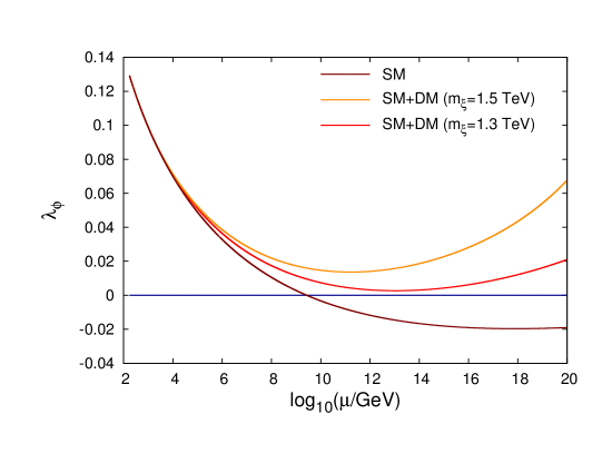
Figure 7: Running SM Higgs quartic coupling in the presence of scalar singlet and fermionic triplet WIMP dark matter as denoted by curves above the horizontal line. The yellow and red curves are for scalar singlet dark matter masses $1.5$ TeV and $1.3$ TeV, respectively. The brown curve is for the SM alone.

7 Baryogenesis Through Leptogenesis

Currently the standard approach towards understanding baryon asymmetry of the Universe (BAU) requires fulfillment of Sakharov[111] conditions: (i) baryon number violation, (ii) C and CP violations, and (iii) departure from thermal equilibrium. BAU is defined as

$$Y_{B}=\frac{n_{B}-n_{\overline{B}}}{s}.$$ (79)

where $n_{B},n_{\overline{B}}$ are number densities of baryons and anti-baryons, respectively, and $s$ is the entropy density. Another equivalent definition of BAU is

$$\eta_{B}=\frac{n_{B}-n_{\overline{B}}}{n_{\gamma}}.$$ (80)

where $n_{\gamma}=$ photon density. Planck satellite experimental values are[6]

$$Y_{B}=8.66\pm 0.11\times 10^{-11},$$ (81)

$$\eta_{B}=6.10\pm 0.08\times 10^{-10}.$$ (82)

Out of various possible mechanisms of baryogenesis such as GUT baryogenesis, electroweak baryogenesis, Affleck-Dyne mechanism, and baryogenesis via leptogenesis [112, 113, 114, 115, 116, 117, 118, 119, 120] we follow leptogenesis path where analogues of Sakharov’s conditions are satisfied.

7.1 CP Asymmetry and Leptogenesis

From the interaction Lagrangian in eq.(45) and eq.(46), it is clear that lepton number violation is possible due to the coexistence of the Dirac neutrino Yukawa matrix $\lambda$ and the Higgs-triplet-bilepton Yukawa matrix $Y$ along with $\mu_{\Delta}$. In general in this model there are two sources of CP asymmetry: (i) decay of RHN to lepton and Higgs pair and (ii) decay of scalar triplet ($\Delta_{L}$) to lepton pair. We point out that the type-II seesaw dominance in SO(10) predicts a class of modified formulas in both these cases where PMNS matrix ($U$) occurs quadratically in the expressions for corresponding CP-asymmetries.

7.1.1 RHN Decay and SO(10) Modified Formula

In the case of RHN decay, the CP asymmetry arises due the interference of the tree level diagram with that of the one loop vertex and self energy diagrams shown in Fig. 8 and Fig.9.

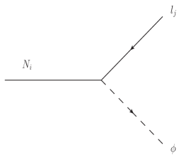
Figure 8: Tree level decay of RHN to lepton and scalar Higgs

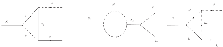
Figure 9: One loop decay diagrams of RHN: (left) vertex correction, (middle) self energy correction, (right) vertex correction due to scalar triplet.

The CP asymmetry [50] produced due to RHN decay is given by

$$\epsilon^{l_{m}}_{N_{k}}=\frac{1}{8\pi(\lambda\lambda^{\dagger})_{kk}}\sum_{j\neq k}\Big{\{}{\cal I}m[(\lambda\lambda^{\dagger})_{kj}\lambda_{km}\lambda_{jm}^{\ast}]g(x_{ij})+{\cal I}m[(\lambda\lambda^{\dagger})_{jk}\lambda_{km}\lambda_{jm}^{\ast}]\frac{1}{1-x_{ij}}\Big{\}}$$ (83)

where $x_{ij}=\frac{M_{N_{j}}^{2}}{M_{N_{i}}^{2}}$ and $g(x)=\sqrt{x}\Big{[}\frac{1}{1-x}+1-(1+x)\ln\Big{(}\frac{1+x}{x}\Big{)}\Big{]}$. The right most diagram of Fig.9 is a new contribution to the CP asymmetry due to loop mediation by $\Delta_{L}$. The corresponding CP asymmetry is given by

$$\epsilon_{N_{k}}^{\Delta^{l_{m}}}=-\frac{1}{2\pi(\lambda\lambda^{\dagger})_{kk}M_{N_{k}}}\sum_{i}{\cal I}m[\lambda_{km}\lambda_{ki}Y_{mi}^{\ast}\mu_{\Delta}]\Big{\{}1-\frac{M_{\Delta}^{2}}{M_{N_{k}}^{2}}\ln\Big{(}1+\frac{M_{N_{k}}^{2}}{M_{\Delta}^{2}}\Big{)}\Big{\}}.$$ (84)

The total CP asymmetry produced due to RHN decay is given by $\epsilon_{N_{k}}^{l_{m}~{}tot}=\epsilon^{l_{m}}_{N_{k}}+\epsilon_{N_{k}}^{\Delta^{l_{m}}}$. For hierarchical RHNs it is sufficient to consider the decay of the lightest RHN neutrino only for $\epsilon_{N_{1}}^{l_{m}~{}tot}$.

The formulas for CP asymmetries presented in eq.(83) and eq.(84) are usually derived [50, 53] under the assumption that the RHNs are in their diagonal basis . But in our type-II seesaw dominance $SO(10)$ models, the light neutrino mass matrix $m_{\nu}\simeq m_{\nu}^{\rm II}=Yv_{L}$ and the RHN mass matrix $M_{N}=YV_{B-L}$. Then these models dictate that the diagonalising matrices for the RHN neutrino mass and the light neutrino mass matrices are one and the same. Thus it forbids a RHN mass diagonal basis of the type [50, 53]. But while calculating the CP asymmetry parameters as we need the RHN masses in their mass basis, this can be realised by the rotation of RHN fields through the mixing matrix $U\simeq U_{\rm PMNS}$). In other words in type-II seesaw dominance SO(10) models the Dirac neutrino Yukawa coupling matrix $\lambda$ will be modified as $\lambda\rightarrow\lambda U^{\ast}$. After inserting this transformation relation, the conventional CP asymmetry formulas of eq.(83) and eq.(84) are modified to assume their new forms

$$\epsilon^{l_{m}}_{N_{k}} = \frac{1}{8\pi(\lambda\lambda^{\dagger})_{kk}}\sum_{j\neq k}\Big{\{}{\cal I}m[(\lambda\lambda^{\dagger})_{kj}(\lambda U^{\ast})_{km}(\lambda^{\ast}U)_{jm}]g(x_{ij})$$

$$+ {\cal I}m[(\lambda\lambda^{\dagger})_{jk}(\lambda U^{\ast})_{km}(\lambda^{\ast}U)_{jm}]\frac{1}{1-x_{ij}}\Big{\}},$$

$$\epsilon_{N_{k}}^{\Delta^{l_{m}}} = -\frac{1}{2\pi(\lambda\lambda^{\dagger})_{kk}M_{N_{k}}}\sum_{i}{\cal I}m[(\lambda U^{\ast})_{km}(\lambda U^{\ast})_{ki}Y_{mi}^{\ast}\mu_{\Delta}]$$ (85)

$$\times \Big{\{}1-\frac{M_{\Delta}^{2}}{M_{N_{k}}^{2}}\ln\Big{(}1+\frac{M_{N_{k}}^{2}}{M_{\Delta}^{2}}\Big{)}\Big{\}}.$$

In the standard model extensions [50, 53], the trilinear scalar coupling $\mu_{\Delta}$ occurring in CP-asymmetry formulas of eq.(84) and eq.(85) is an apriori unknown parameter. But, in our SO(10) models, the origin of this trilinear coupling is traced back to the Higgs scalar quadrilinear interaction between ${10}_{H}$ and ${126}_{H}$ as shown in eq.(48).

7.1.2 Scalar Triplet Decay and SO(10) Modified Formula

The presence of the $Y$ coupling term in eq.(46) allows $\Delta_{L}$ to decay to a lepton pair at the tree level shown in Fig.10. This decay process is also possible at one loop level through vertex correction in the presence of a RHN as shown in the right panel of Fig.10. As we confine to minimal SO(10) models with only one $\Delta_{L}$ we do not discuss one loop self energy correction mediated by two different Higgs scalar triplets [49].

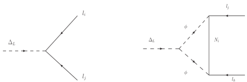
Figure 10: (left panel)tree level and one loop vertex(right panel) diagram of $\Delta_{L}$ decay to lepton pair

In this work our aim is to carry out leptogenesis at different temperature regimes where lepton flavours may be fully or partly distinguishable making the CP asymmetry parameter to explicitly contain lepton flavour indices. We also consider the possibility that the lepton flavours may lose their distinguishability at some higher temperatures. The flavour dependent CP asymmetry which arises due to the interference of the tree level and the vertex correction terms is given by [50, 53]

$$\epsilon_{\Delta}^{l_{i}}=-\frac{1}{4\pi}\sum_{k,j}M_{N_{k}}\frac{{\cal I}m[\mu_{\Delta}Y^{ij}\lambda_{ki}^{\ast}\lambda_{kj}^{\ast}]}{M_{\Delta}^{2}Tr[YY^{\dagger}]+\mu_{\Delta}^{2}}\ln\Big{(}1+\frac{M_{\Delta}^{2}}{M_{N_{k}}^{2}}\Big{)}.$$ (86)

In the type-II seesaw limit $M_{\Delta}\ll M_{N_{k}}$ this formula has been shown to assume a simpler form

$$\epsilon_{\Delta}^{l_{i}}=\frac{M_{\Delta}}{2\pi v^{2}}\frac{\sqrt{B_{l}B_{\phi}}}{\tilde{M_{\Delta}}}{\cal I}m\Big{[}({\cal M}_{\Delta}^{\nu}{{\cal M}_{N}^{\nu}}^{\dagger})_{ii}\Big{]},$$ (87)

where $B_{l},B_{\phi}$, defined through eq.95, are branching ratios of triplet decay to bileptons and two SM Higgs dublets, respectively, and ${\cal M}_{\Delta}^{\nu}$ and ${\cal M}_{N}^{\nu}$ are Type-II, Type-I seesaw mass matrices [53]. Since both the LH$\nu$s and the RHNs are diagonalised by the same unitary matrix $U$ in type-II seesaw dominance SO(10) models, the formula in eq.(86) is also modified

$$\epsilon_{\Delta}^{l_{i}}=-\frac{1}{4\pi}\sum_{k,j}\sum_{m,n}M_{N_{k}}\frac{{\cal I}m[\mu_{\Delta}Y^{ij}\lambda_{km}^{\ast}\lambda_{kn}^{\ast}U_{mi}U_{nj}]}{M_{\Delta}^{2}Tr[YY^{\dagger}]+\mu_{\Delta}^{2}}\ln\Big{(}1+\frac{M_{\Delta}^{2}}{M_{N_{k}}^{2}}\Big{)},$$ (88)

where $\mu_{\Delta}$ is defined through eq.(48). A further necessary consequence is the proportionality ratio between the LH$\nu$ and RHN mass eigen values given in eq.(2) of Sec.1: ${\hat{m}}_{\nu_{1}}:{\hat{m}}_{\nu_{2}}:{\hat{m}}_{\nu_{3}}::{\hat{M}}_{N_{1}}:{\hat{M}}_{N_{2}}:{\hat{M}}_{N_{2}}$. We emphasize that these modifications are consequences of type-II seesaw dominance in SO(10).

In the limit when the mass of the scalar triplet is much lower than the RH neutrino mass eigenvalues $(M_{\Delta}\ll M_{N_{i}})$, the CP asymmetry formula can be simplified a step further to give

$$\epsilon_{\Delta}^{l_{i}}=\frac{M_{\Delta}}{2\pi v^{2}}\frac{\sqrt{B_{l}B_{\phi}}}{\tilde{M_{\Delta}}}{\cal I}m\Big{[}(m_{\nu}^{II}U^{T}{m_{\nu}^{I}}^{\dagger}U)_{ii}\Big{]},$$ (89)

where $m_{\nu}^{I}$ and $m_{\nu}^{II}$ are Type-I, Type-II seesaw mass matrices given in eq.(53) and eq.(56). Explicit form of the parameter $\tilde{M_{\Delta}}$ is given in eq.(107) .

We further emphasize that eq.(85), eq.(88) and eq.(89) are the correct new formulas of CP asymmetry which are valid in the presence of type-II seesaw dominance in SO(10). In the three models being discussed here with RHN masses heavier that $M_{\Delta}$, we have used eq.(88) throughout this work for the prediction of BAU from heavy scalar triplet leptogenesis.

7.2 Boltzmann Equations

In order to get BAU by solving Boltzmann equation we need to take into account only the reactions in the hot plasma whose decay rates at that temperature are comparable to the Hubble rate $\Gamma(T)\sim H(T)$.

The interaction Lagrangian shown in eq.(45) and eq.(46) clearly contains lepton number violating terms. Whenever $N$ decays to $(l,\phi)$ pair or $\Delta_{L}$ decays to $(l_{i},l_{j})$, lepton number is violated by one or two units, respectively. Even though they conserve baryon number, $(B-L)$ is violated in these processes. Our aim is to find out the evolution of $(B-L)$ abundance which at later time gets converted into baryon number through sphaleron interaction. It is worthwhile to mention that for unflavoured leptogenesis $(B-L)$ is conserved by sphalerons whereas for flavoured leptogenesis the conserved quantity in the sphaleron process is $(\frac{B}{3}-L_{i})$. Therefore, for flavoured leptogenesis, we focuss on the evolution of $(\frac{B}{3}-L_{i})$ rather than $(B-L)$. The evolution of $(B-L)$ (or $(\frac{B}{3}-L_{i})$) can not be computed independently but includes evolution of other parameters. As the relevant Boltzmann equations are a set of coupled differential equations, they have to be solved simultaneously in order to get solution for any of the variables. In general the asymmetry can be produced by the decay of both $N$ and $\Delta$ and the set of Boltzmann equations contain first order differentials of RHN density, scalar triplet density and scalar triplet asymmetry. This scalar triplet asymmetry is arising due to the fact that, unlike RHNs, triplets are not self conjugate. The right hand side of relevant Boltzmann equations consists of interaction terms that tend to change the density of the corresponding variables. Taking into account all such interactions, the network of lepton flavour dependent coupled Boltzmann equations are [52, 53]

$$\dot{Y}_{N_{1}}=-\Big{(}\frac{Y_{N_{1}}}{Y_{N_{1}}^{eq}}-1\Big{)}\gamma_{D_{N_{1}}},$$ (90)

$$\dot{Y}_{\Sigma}=-\Big{(}\frac{Y_{\Sigma}}{Y_{\Sigma}^{eq}}-1\Big{)}\gamma_{D}-2\Big{[}\Big{(}\frac{Y_{\Sigma}}{Y_{\Sigma}^{eq}}\Big{)}^{2}-1\Big{]}\gamma_{A},$$ (91)

$$\dot{Y}_{\Delta_{\Delta}}=-\Big{[}\frac{Y_{\Delta_{\Delta}}}{Y_{\Sigma}^{eq}}-\sum_{k}\Big{(}\sum_{i}B_{l_{i}}C_{ik}^{l}-B_{\phi}C_{k}^{\phi}\Big{)}\frac{Y_{\Delta_{k}}}{Y_{l}^{eq}}\Big{]}\gamma_{D},$$ (92)

$$\dot{Y}_{\Delta_{B/3-L_{i}}}=-\Big{[}\Big{(}\frac{Y_{N_{1}}}{Y_{N_{1}}^{eq}}-1\Big{)}\epsilon_{N_{1}}^{l_{i}~{}tot}+\Big{(}\sum_{k}C^{l}_{ik}\frac{Y_{\Delta_{k}}}{Y_{l}^{eq}}+\sum_{k}C^{\phi}_{k}\frac{Y_{\Delta_{k}}}{Y_{l}^{eq}}\Big{)}K^{0}_{i}\Big{]}\gamma_{D_{N_{1}}}$$

$$\hskip 55.48277pt-\Big{[}\Big{(}\frac{Y_{\Sigma}}{Y_{\Sigma}^{eq}}-1\big{)}\epsilon^{l_{i}}_{\Delta}-2\sum_{j}\Big{(}\frac{Y_{\Delta_{\Delta}}}{Y_{\Sigma}^{eq}}-\frac{1}{2}\sum_{k}C^{l}_{ijk}\frac{Y_{\Delta_{k}}}{Y_{l}^{eq}}\Big{)}B_{l_{ij}}\Big{]}\gamma_{D}$$

$$\hskip 55.48277pt-2\sum_{j,k}\Big{(}C^{\phi}_{k}+\frac{1}{2}C^{l}_{ijk}\Big{)}\frac{Y_{\Delta_{k}}}{Y^{eq}_{l}}\Big{(}\gamma^{\prime\phi\phi}_{l_{i}l_{j}}+\gamma^{\phi l_{j}}_{\phi l_{i}}\Big{)}-\sum_{j,m,n,k}C^{l}_{ijmnk}\frac{Y_{\Delta_{k}}}{Y^{eq}_{l}}\Big{(}\gamma^{\prime l_{n}l_{m}}_{l_{i}l_{j}}+\gamma^{l_{m}l_{j}}_{l_{i}l_{n}}\Big{)}~{}~{}.$$

(93)

To specify our notational conventions, $Y_{\Delta_{X}}$ stands for the ratio of number density (or difference of number density) to the entropy density, i.e $Y_{\Delta_{X}}=\frac{n_{X}-n_{\bar{X}}}{s}$, where $n_{X}~{}(n_{\bar{X}})$ is the $X~{}({\bar{X}})$ number density. Expressions for number densities of different particle species $X~{}(\bar{X})$ are given in the Appendix 9.2.1. All the variables of the differential equations $(Y_{N_{1}},Y_{\Delta_{\Delta}},Y_{\Sigma},Y_{\Delta_{B/3-L_{i}}})$ are functions of $z=M_{\Delta}/T$. Therefore, generically, $\dot{Y}_{X}$ denotes $\dot{Y}_{X}\equiv\dot{Y}_{X}(z)=s(z)H(z)\frac{dY_{X}(z)}{dz}$. The scalar triplet density and asymmetry are denoted as $\Sigma=\Delta+\Delta^{\dagger}$ and $\Delta_{\Delta}=\Delta-\Delta^{\dagger}$, respectively. Superscript ‘$eq$’  denotes the equilibrium value of the corresponding quantity. Functional forms of all such equilibrium densities are presented in the Appendix 9.2.1. Here $B_{l}$ and $B_{\phi}$ stand for branching ratio of $\Delta$ decaying to leptons and $\phi\phi$, respectively and $\Gamma_{\Delta}^{tot}$ is the total decay width of $\Delta_{L}$ [53]

$$B_{l}=\sum_{i=e,\mu,\tau}B_{l_{i}}=\sum_{i,j=e,\mu,\tau}B_{l_{ij}}=\sum_{i,j=e,\mu,\tau}\frac{M_{\Delta}}{8\pi\Gamma_{\Delta}^{tot}}|Y^{ij}|^{2},$$ (94)

$$B_{\phi}=\frac{|\mu_{\Delta}|^{2}}{8\pi M_{\Delta}\Gamma_{\Delta}^{tot}},$$

$$\Gamma_{\Delta}^{tot}=\frac{M_{\Delta}}{8\pi}\Big{(}\sum_{i,j}|Y_{ij}|^{2}+\frac{|\mu_{\Delta}|^{2}}{M_{\Delta}^{2}}\Big{)}.$$ (95)

It is obvious that the two branching ratios satisfy $B_{l}+B_{\phi}=1$. Similarly a quantity related to the decay of RHN has been defined, $K_{i}^{0}=\frac{\Gamma(N_{1}\longrightarrow l_{i},\phi)}{\sum_{i}\Gamma(N_{1}\leftrightarrow l_{i},\phi)}$. Here $\gamma_{D}$ is the total reaction density of the triplet including its decay and inverse decay to lepton pair or scalars, and $\gamma_{D_{N_{1}}}$ is the reaction density related to the lightest RHN ($N_{1}$). In this notation $\gamma_{A}$ signifies the gauge induced $2\leftrightarrow 2$ scattering of triplets to fermions, scalars and gauge bosons. Lepton flavour and number $(\Delta L=2)$ violating Yukawa scalar induced $s-$ channel $(\phi\phi\leftrightarrow\bar{l_{i}}\bar{l_{j}})$ and $t-$ channel $(\phi l_{j}\leftrightarrow\bar{\phi}\bar{l_{i}})$ scattering related reaction densities are denoted as $\gamma^{\phi\phi}_{l_{i}l_{j}}$ and $\gamma^{\phi l_{j}}_{\phi l_{i}}$, respectively. Similarly reaction densities related to Yukawa induced triplet mediated lepton flavour violating $2\leftrightarrow 2$ $s-$ channel and $t-$ channel processes are given by $\gamma^{l_{n}l_{m}}_{l_{i}l_{j}}$ and $\gamma^{l_{j}l_{m}}_{l_{i}l_{n}}$, respectively. The primed $s-$ channel reaction densities are given by $\gamma^{\prime}=\gamma-\gamma^{\rm on~{}shell}$. Explicit expressions of these reaction densities are presented in the Appendix 9.2.2. Now the matrices $C^{l}_{ijk}$ and $C^{l}_{ijmnk}$ are defined as[53]

$$C^{l}_{ijk}=C^{l}_{ik}+C^{l}_{jk},$$

$$C^{l}_{ijmnk}=C^{l}_{ik}+C^{l}_{jk}-C^{l}_{mk}-C^{l}_{nk},$$ (96)

where $C^{l}$ matrix relates the asymmetry of lepton doublets with that of $B/3-L_{i}$. Similarly $C^{\phi}$ establishes the relation between the asymmetry of scalar triplet and $B/3-L_{i}$,

$$Y_{\Delta_{l_{i}}}=-\sum_{k}C^{l}_{ik}Y_{\Delta_{k}}$$

$$Y_{\Delta_{\phi}}=-\sum_{k}C^{\phi}_{k}Y_{\Delta_{k}}$$ (97)

where $Y_{\Delta_{k}}$ is the $k-th$ component of the asymmetry vector $\vec{Y}_{\Delta}$ which can be represented as

$$\vec{Y}_{\Delta}\equiv(Y_{\Delta_{\Delta}},Y_{\Delta}{{}_{B/3-L_{k}}})^{T}.$$ (98)

In the above equations $k=1,2,3$ is the generation index for fully (three) flavoured leptogenesis whereas $k=1,~{}2$ for two flavoured leptogenesis and, therefore, the corresponding $\vec{Y}_{\Delta}$ will be a column matrix with four or three entries. The structure of $C^{l}$ and $C^{\phi}$ matrices are determined from different chemical equilibrium conditions. Their detailed structure and dimensionality in different energy regimes are discussed in Appendix 9.2.3.

As the RHN masses in our models are sufficiently heavier than $M_{\Delta}$, their deacy asymmetries are washed out. Thus, neglecting the RHN related quantities, the set of Boltzmann equations are reduced to a simplified form[53]

$$\dot{Y}_{\Sigma}=-\Big{(}\frac{Y_{\Sigma}}{Y_{\Sigma}^{eq}}-1\Big{)}\gamma_{D}-2\Big{[}\Big{(}\frac{Y_{\Sigma}}{Y_{\Sigma}^{eq}}\Big{)}^{2}-1\Big{]}\gamma_{A},$$ (100)

$$\dot{Y}_{\Delta_{\Delta}}=-\Big{[}\frac{Y_{\Delta_{\Delta}}}{Y_{\Sigma}^{eq}}-\sum_{k}\Big{(}\sum_{i}B_{l_{i}}C_{ik}^{l}-B_{\phi}C_{k}^{\phi}\Big{)}\frac{Y_{\Delta_{k}}}{Y_{l}^{eq}}\big{]}\gamma_{D},$$

$$\dot{Y}_{\Delta_{B/3-L_{i}}}=-\Big{[}\Big{(}\frac{Y_{\Sigma}}{Y_{\Sigma}^{eq}}-1\big{)}\epsilon^{l_{i}}_{\Delta}-2\sum_{j}\Big{(}\frac{Y_{\Delta_{\Delta}}}{Y_{\Sigma}^{eq}}-\frac{1}{2}\sum_{k}C^{l}_{ijk}\frac{Y_{\Delta_{k}}}{Y_{l}^{eq}}\Big{)}B_{l_{ij}}\Big{]}\gamma_{D}$$

$$\hskip 55.48277pt-2\sum_{j,k}\Big{(}C^{\phi}_{k}+\frac{1}{2}C^{l}_{ijk}\Big{)}\frac{Y_{\Delta_{k}}}{Y^{eq}_{l}}\Big{(}\gamma^{\prime\phi\phi}_{l_{i}l_{j}}+\gamma^{\phi l_{j}}_{\phi l_{i}}\Big{)}-\sum_{j,m,n,k}C^{l}_{ijmnk}\frac{Y_{\Delta_{k}}}{Y^{eq}_{l}}\Big{(}\gamma^{\prime l_{n}l_{m}}_{l_{i}l_{j}}+\gamma^{l_{m}l_{j}}_{l_{i}l_{n}}\Big{)}~{}~{}.$$

(101)

Simultaneous solution of above three equations enable us to know the value of the asymmetry parameters $(Y_{\Delta_{B/3-L_{i}}})$ at high value of $z$ where the value of the asymmetry gets frozen. Then the final value of the baryon asymmetry is

$$Y_{\Delta_{B}}=3\times\frac{12}{37}\sum_{i}Y_{\Delta_{B/3-L_{i}}},$$ (102)

where the factor $3$ signifies the degrees of freedom of $\Delta_{L}$.

When the temperature is above $10^{12}$ GeV, different lepton flavours lose their distinguishability. Therefore the corresponding Boltzmann equations are free of lepton flavour indices. This variant of leptogenesis is referred to as the unflavoured leptogenesis and the set of Boltzmann equations in eq.(100)-eq.(101) are modified [53]

$$\dot{Y}_{\Sigma}=-\Big{(}\frac{Y_{\Sigma}}{Y_{\Sigma}^{eq}}-1\Big{)}\gamma_{D}-2\Big{[}\Big{(}\frac{Y_{\Sigma}}{Y_{\Sigma}^{eq}}\Big{)}^{2}-1\Big{]}\gamma_{A}$$ (103)

$$\dot{Y}_{\Delta_{\Delta}}=\Big{[}\frac{Y_{\Delta_{\Delta}}}{Y_{\Sigma}^{eq}}-\sum_{k}\Big{(}B_{l}C_{k}^{l}-B_{\phi}C_{k}^{\phi}\Big{)}\frac{Y_{\Delta_{k}}}{Y_{l}^{eq}}\big{]}\gamma_{D},$$ (104)

$$\dot{Y}_{\Delta_{B-L}}=-\Big{[}\Big{(}\frac{Y_{\Sigma}}{Y_{\Sigma}^{eq}}-1\big{)}\epsilon^{l}_{\Delta}-2\Big{(}\frac{Y_{\Delta_{\Delta}}}{Y_{\Sigma}^{eq}}-\sum_{k}C^{l}_{k}\frac{Y_{\Delta_{k}}}{Y_{l}^{eq}}\Big{)}B_{l}\Big{]}\gamma_{D}$$

$$\hskip 45.52458pt-2\sum_{k}\Big{(}C^{\phi}_{k}+C^{l}_{k}\Big{)}\frac{Y_{\Delta_{k}}}{Y^{eq}_{l}}\Big{(}\gamma^{\prime\phi\phi}_{ll}+\gamma^{\phi l}_{\phi l}\Big{)},$$ (105)

where $\epsilon^{l}_{\Delta}~{}(=\sum_{i}\epsilon^{l_{i}}_{\Delta})$ is the flavour summed or unflavoured CP asymmetry parameter and the asymmetry vector $\vec{Y}_{\Delta}$ is now reduced to a column vector with only two entries, $\vec{Y}_{\Delta}^{T}=(Y_{\Delta_{\Delta}},Y_{\Delta_{B-L}})$. Thus, in this case also, the final baryon asymmetry is computed using the simple formula of eq.(102).

7.3 Parameter Space for Leptogenesis

Whether the lepton flavours should be treated separately depends entirely on the phenomenon of flavour decoherence which is generally assumed [53] to occur when lepton Yukawa rate becomes faster than the Hubble rate at that very temperature. Some deeper considerations are needed to avoid possibility of resulting over simplication.

In the model with SM + three RHNs + one triplet $\Delta_{L}$ [53] , the flavour decoherence issue is mainly dictated by the competition of two reactions: SM lepton Yukawa interaction and inverse decay of lepton to triplet $\Delta_{L}$. To make this point clear let us suppose that at certain temperature $(T_{h})$ during the evolution of universe , the lepton Yukawa interaction becomes faster than the Hubble rate, whereas the triplet inverse decay $(ll\rightarrow\bar{\Delta})$ rate is faster than the lepton Yukawa interaction rate. As a result the charged leptons will inverse decay before they can undergo any charged lepton Yukawa interaction. Thus separate identity for different lepton flavours still can not be understood. At some lower temperature the inverse decay rate is reduced since it is Boltzmann suppressed. At a temperature $T=T_{decoh}$, when the inverse decay rate becomes smaller than the lepton Yukawa interaction rate, the decoherence between the lepton flavours is fully achieved. So between the temperature range $(T_{h}-T_{decoh})$ the flavour decoherence is not fully achieved, i.e within this intermediate temperature regime we should not use flavoured leptogenesis formalism.

The decoherence temperature $(T_{decoh})$ is determined by the mass of the scalar triplet $(M_{\Delta})$ and effective decay parameter[53]

$$\tilde{M}_{\Delta}^{eff}=\tilde{M}_{\Delta}\sqrt{\frac{1-B_{\phi}}{B_{\phi}}},$$ (106)

where

$$\tilde{M}_{\Delta}^{2}=|\mu_{\Delta}|^{2}\frac{v^{4}}{M_{\Delta}^{4}}Tr[YY^{\dagger}],$$ (107)

and $B_{\phi}$ is branching ratio of triplet decay to scalar doublets $\phi\phi$.

Decoherence can be fully achieved when our chosen parameter space satisfies the condition that, at a given temperature, lepton triplet inverse decay rate is slower than the SM lepton Yukawa interaction rate. By imposing this condition we can get an upper limit on $M_{\Delta}$ as a function of $\tilde{M}_{\Delta}^{eff}$

$$\Gamma_{f_{i}}\geq B_{l}\Gamma_{\Delta}^{tot}\frac{Y_{\Sigma}^{eq}}{Y_{l}^{eq}}~{}~{}~{}~{}~{}~{}({~{}f_{i}=\tau,\mu}).$$ (108)

This constraint relation can be translated into constraints over $M_{\Delta}$ and $\tilde{M}_{\Delta}^{eff}$ [53]

$$M_{\Delta}\leq 4\times\Big{(}\frac{10^{-3}{\rm eV}}{\tilde{M}_{\Delta}^{eff}}\Big{)}\times 10^{11}~{}~{}{\rm GeV}~{}~{}~{}~{}({\rm fully~{}two~{}flavoured}),$$ (109)

$$M_{\Delta}\leq 1\times\Big{(}\frac{10^{-3}{\rm eV}}{\tilde{M}_{\Delta}^{eff}}\Big{)}\times 10^{9}~{}~{}{\rm GeV}~{}~{}~{}~{}({\rm fully~{}three~{}flavoured})~{}~{}.$$ (110)

In Fig.(11) we have shown the allowed parameter space for different regimes depending upon viability of various kinds of (flavoured/unflavoured) leptogenesis.

It is essential to state the conditions which have been used here to generate the parameter space. By changing the value of two free parameters $(\mu_{\Delta},M_{\Delta})$ in every model we are able to vary all such parameters which implicitly or explicitly depend upon them. The number of points in the allowed parameter space ($M_{\Delta}$ vs $\tilde{M}_{\Delta}^{eff}$) is reduced due to imposition of two constraint relations as given below.

The Type-II seesaw dominance condition which is valid in all SO(10) models is $\frac{|Yv_{L}|}{M_{D}M_{N}^{-1}M_{D}^{T}}\gg 1$. Considering both real and imaginary parts, this condition gives

$$Re(m_{\nu}^{I})_{ij}\ll Re(Yv_{L})_{ij}$$

$$Im(m_{\nu}^{I})_{ij}\ll Im(Yv_{L})_{ij}.$$ (111)

We estimate reaction densities $\gamma_{D}$ and $\gamma_{D_{N_{1}}}$ with only those points which satisfy the condition of eq.(111). Then we choose only those points which satisfy

$$\gamma_{D_{N_{1}}}\ll\gamma_{D}$$ (112)

for each and every value in the whole range of $z=0-100$. Fulfillment of this second constraint relation allows us to neglect all RHN related quantities in eq.(90)-eq.(93). Then the estimated leptogenesis is due to the decay of scalar triplet in a type-II seesaw dominated SO(10) model.

At first we present the parameter space of $M_{\Delta}$ vs $\tilde{M}_{\Delta}^{eff}$ depicting different leptogenesis regimes depending upon distinguishability of lepton flavors without imposing any constraint on $\tilde{M}_{\Delta}^{eff}$ and $M_{\Delta}$. We vary $M_{\Delta}$ (in the range $(10^{5}~{}-~{}10^{9})$ GeV) and $\tilde{M}_{\Delta}^{eff}$ in the range $(10^{-6}~{}-~{}10^{9})$ eV independent of each other. Then, depending upon the constraint relations in eq.(109) and eq.(110), we place the set of points in different leptogenesis regimes and designate them with different colours.

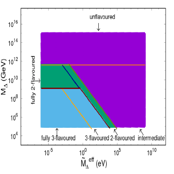
Figure 11: Allowed parameter space depicting the region of viability of different kinds of leptogenesis without any constraint on $\tilde{M}_{\Delta}^{eff}$ and $M_{\Delta}$

The significance of different regimes shown in the plot of Fig. 11 can be explained as follows. The horizontal lines at $(M_{\Delta}\sim 10^{9})$ GeV and $(M_{\Delta}\sim 10^{12})$ GeV basically indicate that above the corresponding values of $M_{\Delta}$, the $\mu$ and $\tau$ Yukawa interactions can never reach thermal equilibrium which simply means that above $M_{\Delta}\sim 10^{12}$ GeV we can not separate any of the flavours. Similarly, above $(M_{\Delta}\sim 10^{9})$ GeV, $\mu$ and $e$ flavours can never be distinguished. Thus it is not possible to have fully flavoured or three flavoured leptogenesis above $(M_{\Delta}\sim 10^{9})$ GeV and 2-flavoured leptogenesis above $(M_{\Delta}\sim 10^{12})$ GeV. The points in the sky-blue region are obtained as fully three flavoured using eq.(110) and the points in the green region are obtained as fully two flavoured using eq.(109). Both the regions are further constrained by the condition that $\tau$(or $\mu$) Yukawa interaction is always faster than the $ll\rightarrow\Delta$ inverse decay rate.
Tiny patches labeled as three flavoured and two flavoured are obtained by the fulfillment of the condition that $\tau$ or $\mu$ Yukawa interaction is faster than the $ll\rightarrow\Delta$ inverse decay rate when $z>z_{A}$ where $z_{A}=\frac{M_{\Delta}}{T_{A}}$, $T_{A}$ being the temperature where the gauge scattering rate is slower than the decay rate.
The intermediate regime is little bit tricky. Here depending upon the choice of the parameters $M_{\Delta}$ and $\tilde{M}_{\Delta}^{eff}$ at first we have to calculate $T^{\tau}_{decoh}$. If $T>T^{\tau}_{decoh}$ we would have a unflavoured scenario whereas $T<T^{\tau}_{decoh}$ leads us to two-flavoured scenario.

We now proceed to calculate the quantity $\tilde{M}_{\Delta}^{eff}$ thoroughly following the model under consideration by imposing the Type-II seesaw dominance. Then we represent the parameters $\tilde{M}_{\Delta}^{eff}$ and $M_{\Delta}$ graphically again and show the effect of imposition of Type-II seesaw dominance constraint. Here we vary $M_{\Delta}$ in the range $(10^{9}~{}-~{}10^{15})$ GeV following the gauge coupling unification constraints $M_{\Delta}>10^{9.2}$ GeV ( Model-I ), $M_{\Delta}>10^{10.2}$ GeV ( Model-II ), and $M_{\Delta}>10^{10.4}$ GeV ( Model-III ).

In order to ensure that self-energy correction term does not exceed the tree level term, we use vlues of $\mu_{\Delta}\leq M_{\Delta}$. Thereafter, imposing Type-II seesaw dominance, we find values of $\tilde{M}_{\Delta}^{eff}$ corresponding to each set of points $(M_{\Delta},\mu_{\Delta})$ using eq.(107) that also needs the $Y$ matrix which is proportional to $m_{\nu}$. Choosing the mass eigenvalue of a light neutrino, we estimate the other two mass eigenvalues. Then using $3\sigma$ values of mixing angles and any two values of the Dirac phase $\delta$ we generate a number of sets for $m_{\nu}$ using eq.(57). Here we present graphically the parameter space for only those points which at the end produce acceptable values of baryon asymmetry in the $3\sigma$ range. Armed with all these quantities finally we are able to calculate $\tilde{M}_{\Delta}^{eff}$ for each set of values of $(M_{\Delta},\mu_{\Delta})$. For a fixed set of oscillation parameters, in this method $\tilde{M}_{\Delta}^{eff}$ varies with the location of the point $(M_{\Delta},\mu_{\Delta})$. Then using the constraint relations in eq.(109) and eq.(110), we subdivide the allowed values of $(M_{\Delta},\mu_{\Delta})$ into different regimes of leptogenesis.
We carry out the above mentioned exercise for both normal and inverted orderings and the corresponding plots are shown in the Fig. 12.

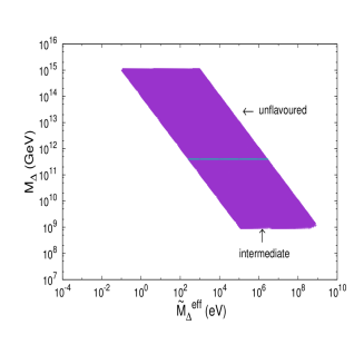
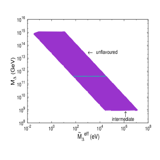
Figure 12: Viable regions of parameter space for different kinds of leptogenesis in the case of (a) normal hierarchy with $\delta=170^{\circ}$ (left panel),(b) inverted hierarchy with $\delta=200^{\circ}$ (right-panel).

In the present context, a pertinent question to ask is whether it is acceptable to use a single leptogenesis formalism such as unflavoured, or 2-flavoured, or 3-flavoured cases and the corresponding single set of Boltzmann equations for the whole $z$ range. Asymmetry is mainly produced at an epoch when $z>z_{A}$. In this situation if we have $z_{A}>z^{\tau}_{decoh}$(or $z_{A}>z^{\mu}_{decoh}$), then it is justified to use 2-flavoured (or 3-flavoured) leptogenesis formalism for the whole range of $z$. We have checked that in the entire violet region of the parameter space of Fig.12 we can use the unflavoured leptogenesis formalism.

The plots given in Fig. 12 are generated by only those points which satisfy the two constraint relations, eq.(111) and eq.(112). Our leptogenesis estimations are then carried out for the points belonging to this parameter space only. Thus in our type-II dominated SO(10) where $\Delta_{L}$ related quantities are important, the corresponding set of Boltzmann equation is rightly chosen to be eq.(103)-eq.(105).

It is clear from Fig. 12 that the allowed parameter space has been reduced considerably, compared to Fig. 11, due to imposition of the Type-II dominance constraint. Since unification of coupling constants forbids us to take $M_{\Delta}$ below $10^{9}$ GeV, the 3-flavoured regime is automatically discarded. The reason behind such huge reduction of parameter space can be explained through some simple mathematical arguments. In our numerical analysis the light neutrino mass matrix is due to type-II seesaw $m_{\nu}\simeq Yv_{L}$. The light neutrino mass matrix is already known to us since we know the mass eigenvalues and mixing angles from oscillation data. So $Y$ matrix is known from $Y=(1/v_{L})m_{\nu}$. Again the RH neutrino mass matrix can be expressed as $M_{N}\simeq m_{\nu}\frac{V_{B-L}}{v_{L}}$. Now we are able to find order of magnitude values of type-I remnant along with dominant Type-II contribution. Varying $(M_{\Delta},\mu_{\Delta})$ we can get different values of $Y$ matrix and $M_{N}$ matrices. We allow only those set of values of $(M_{\Delta},\mu_{\Delta})$ which are compatible with the Type-II dominance constraint. We have introduced the Type-II dominance condition in our analysis by imposing

$$\frac{(Yv_{L})_{ij}}{(M_{D}^{T}M_{N}^{-1}M_{D})_{ij}}>10~{}.$$ (113)

Expressing $M_{N}$ in terms of $m_{\nu}$ the above equation can be rewritten to express the Type-II dominance condition

$$Y_{ij}>\frac{10}{V_{B-L}}(M_{D}^{T}(m_{\nu})^{-1}M_{D})_{ij}~{}.$$ (114)

We have used the SO(10) prediction for Dirac neutrinino mass $M_{D}=M_{u}=$ up-quark mass. For NO case we have taken $V_{B-L}\geq 4\times 10^{17}$GeV. Since numerical values of each quantities in the RHS of above equation are known, we can have a fair idea about the magnitude of $Y$ matrix needed for Type-II seesaw dominance. Exact numerical values are presented in the Appendix 9.2.4.

We now try to analyse the effect of constraint eq.(109) on $M_{\Delta}$ and ${\tilde{M}}_{\Delta}^{eff}$ which has to be satisfied in order to be in the fully 2-flavoured regime. Our aim is to express the constraint equation in terms of $Y$ matrix such that we can infer whether the same $Y$ is simultaneously compatible with type-II dominance eq.(114) and the condition to be in the fully 2-flavoured regime. The expression of $\tilde{M}_{\Delta}^{eff}$ eq.(106) through eq.(107) can be simplified by expressing the branching ratio $B_{\phi}$ in terms of the $Y$ matrix leading to

$$\tilde{M}_{\Delta}^{eff}=\frac{v^{2}}{M_{\Delta}}Tr[YY^{\dagger}]\times 10^{9}~{}~{}{\rm eV}.$$ (115)

Using this form of ${\tilde{M}}_{\Delta}^{eff}$ in the constraint relation of eq.(109) for fully 2-flavoured regime, we get the limiting values of Yukawa couplings

$$Tr[YY^{\dagger}]\leq 6.6\times 10^{-6}.$$ (116)

Thus a point will be in the fully 2-flavoured regime if the conditions in eq.(114) and eq.(116) are simultaneously satisfied. In actual numerical estimations, as we have shown in Appendix 9.2.4) for both the NO and IO cases, it is not at all possible to satisfy these two constraint relations given in eq.(114) and eq.( 116) simultaneously. Consequently, the two- flavoured regime is disallowed both in NO and IO cases. In this way we can justify the restricted region presented in Fig. 12.

7.4 Remarks on Baryon Asymmetry Estimation

We now estimate baryon asymmetry using the points belonging to the parameter space shown in Fig. 12. Out of large number of available choices we pick some representative points from each regime for BAU estimation. Although allowed parameter space has been shown in the $M_{\Delta}$ vs. $\tilde{M}_{\Delta}^{eff}$ plot, this can be translated into $(M_{\Delta}$ vs. $\mu_{\Delta})$ plot as there is a one-to-one correspondence between the sets: $(M_{\Delta},\mu_{\Delta})\rightarrow(M_{\Delta},\tilde{M}_{\Delta}^{eff})$. It is obvious that while demanding that we are taking a point $(M_{\Delta},\mu_{\Delta})$ from the unflavoured regime implies that the corresponding $(M_{\Delta},\tilde{M}_{\Delta}^{eff})$ will definitely fall in the unflavoured regime of $M_{\Delta}$ vs $\tilde{M}_{\Delta}^{eff}$ plot.

Few important remarks are in order before actual computation. The parameter space shown in Fig. 12 are obtained by varying $(M_{\Delta},\mu_{\Delta})$ while keeping $m_{\nu}$ fixed at its best fit value as given in eq.(59) for NO and in eq.(61) for IO. These best fit values include mass squared differences, mixing angles, and the Dirac CP phases. The value of the Dirac CP phase $(\delta)$ has not been measured with desired accuracy till date. Therefore, apart from the central value as given in Table 6, we have carried out our analysis also for another choice $\delta=170^{\circ}$ in the case of NO. In Fig. 12 we have shown plots for only that value of $\delta$ which at the end produces positive value of baryon asymmetry $(Y_{B})$.

On the requirement of CP-asymmetry parameters we note that, in the fully flavoured, 2-flavoured and unflavoured regimes, we need three, two and one CP asymmetry parameters, respectively. Final value of the generated baryon asymmetry depends crucially upon the sign and magnitude of these CP asymmetry parameters. The magnitude of CP asymmetry parameters mainly depends on the mass of the decaying particle which increases with the particle mass. The sign of the CP asymmetry parameters depends on the relative phases between the coupling matrices $\lambda$ and $Y$. As the phase of $\lambda$ in the chosen up quark diagonal bvasis are fixed. We can tune the phases of $Y$ matrix by taking different values of the Dirac CP phase $\delta$. As a result the sign of CP asymmetry parameter can be changed by changing the value of $\delta$ leading to a positive value of the asymmetry parameter $Y_{B}$.

7.5 Baryon Asymmetry for Normal Ordering

Here at first we calculate baryon asymmetry taking the points within the whole violet region corresponding to unflavoured +intermediate regime of the left panel in Fig. 12 which is consistent with neutrino data for $\delta=170^{\circ}$. When we find unacceptable solutions within best fit values of $\delta$, we extend our search region covering its $3\sigma$ range as quoted in Table 6.

7.5.1 Unflavoured Regime

This regime is composed of all the points of the region denoted as unflavoured as well as most of the points from the region labeled as intermediate. With these points we calculate the flavour independent CP asymmetry parameters $(\epsilon^{l}_{\Delta}=\sum_{i}\epsilon^{l_{i}}_{\Delta})$ and plug them into the set of unflavoured Boltzmann equations, eq.(103)-eq.(105), which are then solved to get the final value of $(B-L)$ asymmetry. This $(B-L)$ asymmetry is then converted into baryon asymmetry through sphaleron process through the formula of eq.(102). Other ingredients required for solving the Boltzmann equations are $C^{l}$ and $C^{\phi}$ matrices discussed in Appendix Sec. 9.2.3. We carry out our analysis with some of the chosen points from the unflavoured regime as depicted in the left panel of Fig. 12. For these chosen points the CP asymmetry parameter is found to be negative and the $(B-L)$ asymmetry parameter $Y_{B}$ also freezes to a positive value for high $z$ in agreement with Planck satellite data [6] given in eq.(81) and eq.(82). We note that there are a plenty of points in this regime having such acceptable solutions.

Table 8: Numerical values of parameters for NO in the unflavoured regime which can produce $Y_{B}\sim 8.6\times 10^{-11}$ with best fit values of the neutrino mass eigenvalues, mixings and $\delta=170^{\circ},\alpha_{M}=0,\beta_{M}=0$.

$M_{N_{1}}/10^{16}$ (GeV)	$1.084$	$1.087$	$1.09$	$1.09$
$M_{\Delta}/10^{14}$ (GeV)	$9.5$	$9.6$	$9.7$	$9.8$
$\mu_{\Delta}/10^{14}$ (GeV)	$5.5$	$5.6$	$5.7$	$5.8$
$\tilde{M}_{\Delta}^{eff}\times 10^{2}$ (eV)	$0.121$	$0.120$	$0.120$	$0.119$
$Y_{B}\times 10^{11}$	$8.53$	$8.60$	$8.67$	$8.71$

In Table 8 we have shown some of these points. In the left panel of Fig. 13 we plot allowed values of $M_{\Delta}$ vs. $\mu_{\Delta}$ representing solutions $Y_{B}\sim 8.6\times 10^{-11}$). In the right panel of Fig. 13 we present the variation of $Y_{B}$ ( $=Y_{B-L}$) with $z$. Form the plot it is clear that $Y_{B}$ indeed freezes to its experimentally observed value for large $z$.

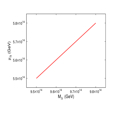
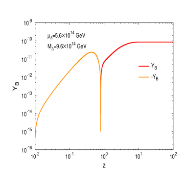
Figure 13: Plot of set of pints $(M_{\Delta}{\rm vs.}\mu_{\Delta})$ required to produce $Y_{B}$ in the experimental range (left panel) and variation of $Y_{B}$ with $z$ for a definite value of $(M_{\Delta},\mu_{\Delta})$ (right panel). For these NO solutions best fit values of the neutrino mass eigenvalues and mixings have been used with phases $\delta=170^{\circ},\alpha_{M}=0,\beta_{M}=0$.

The whole numerical analysis and successful $Y_{B}$ solutions have been obtained for best fit values of neutrino data with Dirac phase $\delta=170^{\circ}$ but with vanishing Majorana phases. But in the presence of type-II seesaw dominance in SO(10), as there is a one-to-one correspondence between $Y$ and $m_{\nu}$ , the effect of any non-vanishing Majorana phases or a different Dirac phase can be easily analysed. In Table 9 we have estimated the type-I seesaw remnant mass eigen values $m_{\nu_{1}}^{I},m_{\nu_{2}}^{I},m_{\nu_{3}}^{I}$ corresponding to our chosen parameter space. Their negligible values compared to neutrino data confirms our type-II seesaw dominance approximation also numerically.

Table 9: Type-I seesaw remnant contribution to neutrino mass eigenvalues for some specific set of parameters in concordance with type-II seesaw dominance and BAU with best fit for neutrino data with NO eigen values and $\delta=170^{\circ},$ and $\alpha_{M}=0,\beta_{M}=0$.

$M_{\Delta}/10^{14}$ (GeV)	$9.5$	$9.6$	$9.7$	$9.8$
$\mu_{\Delta}/10^{14}$ (GeV)	$5.5$	$5.6$	$5.7$	$5.8$
$M_{N_{1}}/10^{16}$ (GeV)	$1.084$	$1.087$	$1.091$	$1.094$
$M_{N_{2}}/10^{16}$ (GeV)	$9.381$	$9.409$	$9.437$	$9.467$
$M_{N_{3}}/10^{17}$ (GeV)	$5.444$	$5.460$	$5.477$	$5.494$
$m_{\nu_{1}}^{I}$ (eV)	$6.15\times 10^{-15}$	$6.13\times 10^{-15}$	$6.11\times 10^{-15}$	$6.09\times 10^{-15}$
$m_{\nu_{2}}^{I}$ (eV)	$2.13\times 10^{-10}$	$2.13\times 10^{-10}$	$2.12\times 10^{-10}$	$2.11\times 10^{-10}$
$m_{\nu_{3}}^{I}$ (eV)	$1.86\times 10^{-4}$	$1.85\times 10^{-4}$	$1.85\times 10^{-4}$	$1.84\times 10^{-4}$

As an example we have repeated the whole procedure using the best fit values of neutrino data but with a different set of phases $\alpha_{M}=45^{\circ},\beta_{M}=45^{\circ}$ and $\delta=270^{\circ}$. Numerical solutions are presented in Table 10 consistent with baryon asymmetry value $Y_{B}\sim 8.6\times 10^{-11}$. In the left panel of Fig.14 we present allowed values of $M_{\Delta}$ and $\mu_{\Delta}$ consistent with eq.(81) and in the right panel we show variation of $Y_{B}$ with $z$ for a specific set of values of $(M_{\Delta},\mu_{\Delta})$.

Table 10: Numerical values of parameters in the unflavoured regime consistent with $Y_{B}\sim 8.6\times 10^{-11}$ and best fit values of NO neutrino mass eigenvalues, mixings and phases $\delta=270^{\circ},\alpha_{M}=45^{\circ},\beta_{M}=45^{\circ}$.

$M_{N_{1}}/10^{16}$ (GeV)	$0.60$	$1.19$	$2.01$	$2.51$	$2.84$	$3.06$	$3.2$
$M_{\Delta}/10^{14}$ (GeV)	$0.71$	$1.7$	$3.4$	$4.7$	$5.6$	$6.2$	$6.6$
$\mu_{\Delta}/10^{13}$ (GeV)	$0.55$	$1.6$	$3.8$	$0.58$	$0.73$	$0.83$	$0.90$
$\tilde{M}_{\Delta}^{eff}\times 10^{2}$ (eV)	$0.50$	$0.82$	$1.16$	$1.32$	$1.41$	$1.48$	$1.52$
$Y_{B}\times 10^{11}$	$8.6$	$8.65$	$8.52$	$8.65$	$8.71$	$8.62$	$8.61$

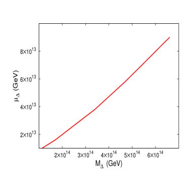
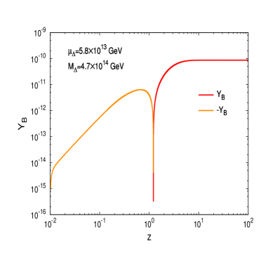
Figure 14: Plot of allowed values of $(M_{\Delta},\mu_{\Delta})$ required to produce $Y_{B}$ in the experimental range (left panel) and variation of $Y_{B}$ with $z$ for a definite set of allowed values of $(M_{\Delta},\mu_{\Delta})$ (right panel). In this NO case best fit to neutrino data has been used with phases $\delta=270^{\circ},\alpha_{M}=45^{\circ},\beta_{M}=45^{\circ}$.

Few remarks on the choice of the SO(10) (or $U(1)_{B-L}$) breaking VEV $V_{B-L}=4\times 10^{17}{\rm GeV}$  are in order. Here we have ensured type-II seesaw dominance by comparing each of the type-II matrix element with the corresponding element in type-I seesaw. To get successful leptogenesis with $Y_{B}\sim 8\times 10^{-11}$), we have also taken $V_{B-L}\geq 4\times 10^{17}$ GeV, but a choice below this VEV may lead to $Y_{B}$ values less tan the Planck[6] data.

Since two-flavoured and three flavoured regimes are not allowed in our type-II seesaw dominance models as discussed in Sec.7.3, we do not discuss methodology for estimation of BAU in these two cases.

7.6 Baryon Asymmetry for Inverted Ordering

In Fig. 12 (right panel) we have clarified why the IO case allows only unflavoured regime which we utilise here to predict BAU.

We choose some representative points from the unflavoured and intermediate regime depicted as the violet area of right panel in Fig. 12. Then following the same steps as NO case, we estimate the asymptotic value of $Y_{B}$ for large enough value of $z$. In this case, apart from using best fit values of IO mass eigen values and mixings, we have also explored possibility of solutions within $3\sigma$ allowed range of Dirac CP phase. We have estimated the CP asymmetry parameter for $\delta=284^{\circ}$ which is in the fourth quadrant and is the best fit value [3, 4], and for $\delta=200^{\circ}$ which is in the third quadrant. For $\delta=284^{\circ}$ the estimated CP asymmetry comes out to be positive which yields negative value of baryon asymmetry $Y_{B}$ at a large enough value of $z$. On the other hand using $\delta=200^{\circ}$ we get negative value of CP asymmetry parameter and, consequently, we get positive value of $Y_{B}$. in agreement with Planck satellite data.

Table 11: Numerical values of parameters in the unflavoured regime which can produce $Y_{B}\sim 8.6\times 10^{-11}$ consistent with best fit values of IO neutrino mass eigenvalues, mixings and phases $\delta=200^{\circ},\alpha_{M}=0,\beta_{M}=0$.

$M_{N_{1}}/10^{16}$ (GeV)	$8.92$	$12.03$	$14.26$	$17.62$	$20.55$	$22.29$	$24.53$	$36.20$
$M_{\Delta}/10^{13}$ (GeV)	$1.9$	$3.0$	$3.9$	$5.5$	$7.1$	$8.10$	$9.50$	$18.00$
$\mu_{\Delta}/10^{11}$ (GeV)	$3.3$	$6.1$	$8.7$	$14.0$	$20.0$	$24.00$	$30.00$	$73.00$
$\tilde{M}_{\Delta}^{eff}$ (eV)	$5.14$	$5.92$	$6.39$	$6.92$	$7.30$	$7.53$	$7.77$	$8.93$
$Y_{B}\times 10^{11}$	$8.6$	$8.65$	$8.57$	$8.60$	$8.66$	$8.64$	$8.67$	$8.66$

In Table 11 we present only those points which produce $Y_{B}$ in agreement with experimental data. In Fig.15 (left panel) we depict the values of $\mu_{\Delta}$ and $M_{\Delta}$ for which $Y_{B}\sim 8\times 10^{-11}$. We choose one such combination of $(\mu_{\Delta},M_{\Delta})$ from the $\mu_{\Delta}$ vs $M_{\Delta}$ plot and show the variation of $Y_{B}$ with $z$. This is presented by the right panel of Fig.15.

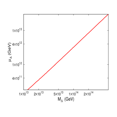
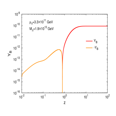
Figure 15: Plot of some allowed set of points $(M_{\Delta},\mu_{\Delta})$ required to produce $Y_{B}$ in the experimental range (left panel) and variation of $Y_{B}$ with $z$ for a definite value of $(M_{\Delta},\mu_{\Delta})$ (right panel). In this IO case best fit values of neutrino data have been used with phases $\delta=200^{\circ},\alpha_{M}=0,\beta_{M}=0$.

From the systematic analysis of leptogenesis presented in the above sections it is inferred that positive baryon asymmetry in the experimentally observed range can be produced using best fit values of neutrino oscillation observables with a large Dirac CP phase in type-II seesaw dominated SO(10) scenario where the lepton asymmetry is generated mainly due to the decay of the left handed scalar triplet and this observation holds both for normal and inverted orderings of neutrino masses. We also find that predicted values of BAU are in concordance with $\theta_{23}$ in the second octant.

8 Summary and Conclusion

In this work we have addressed six limitations of the standard model: (i) Neutrino mass, (ii) Baryon asymmetry of the Universe, (iii) Origin of dark matter and its stability, (iv) Vacuum stability of SM scalar potential, (iv) Origin of three gauge forces of SM, and (vi) Experimentally observed proton stability. For this purpose we have successfully constructed three different type-II seesaw dominance models using the symmetry breaking pattern SO(10) $\to$ SU(5) $\to$ SM which unify gauge couplings and predict the mass of LH triplet scalar $\Delta_{L}$ mediating type-II seesaw to be lighter than RHN masses and the SU(5) unification scale. Manifestly, each of these models allows type-II seesaw dominance and triplet leptogenesis. SO(10) breaking through ${126}_{H}$ predicts matter parity ($Z_{MP}$) as stabilising gauged discrete symmetry for its non-standard fermionic (scalar) DM components with even (odd) value of $Z_{MP}$. Neither these intrinsic DM properties, nor the coupling unification can be predicted in SM extensions [8, 53]. In our SO(10) models the same Majorana Yukawa coupling matrix $Y$ defines the matricial structures of both the type-II seesaw and the RHN mass matrices. As a result the same PMNS matrix ($U$) that diagonalises the neutrino mass matrix in the type-II seesaw dominance approximation also diagonalises the RHN mass matrix. This prevents the freedom of choosing a RHN diagonal basis used in [53]. Further the underlying quark lepton symmetry of SO(10) predicts the Dirac neutrino Yukawa coupling from the up-quark mass matrix $\lambda\simeq\sqrt{2}M_{u}/v$ which is unknown in SM extension [53]. In addition, as the SO(10) breaking VEV $V_{B-L}\geq 10^{17}$ GeV and the known Majorana coupling matrix $Y$ also determine the RHN mass matrix in our models, the type-I seesaw remnant occurring in the CP-asymmetry formula is also known. These predictions and constraints specific to type-II seesaw dominance in SO(10) are naturally absent in the SM extensions [53]. Thus, for realisation of leptogenesis in the presence of type-II seesaw dominance in SO(10), we predict a new class of CP-asymmetry formulas which have been explicitly stated through eq.(85), eq.(88) and eq.(89) in the corresponding cases. As the three RHNs are fundamental to SO(10) unification, unlike the SM extension [53], our models do not predict purely triplet leptogenesis with only LH triplets excluding RHNs. Rather they predict RHN loop mediated triplet leptogenesis. Despite these constraints, all our models predict right value of baryon asymmetry in agreement with Planck data [6] for both NO and IO neutrino masses through unflavoured leptogenesis. Another important outcome of these new SO(10) models is that their type-II seesaw dominance is capable of fitting any neutrino data including $\theta_{23}$ in the second octant and Dirac and/or Majorana phases. In Model-I and Model-II, we have further predicted a real scalar DM candidate of mass $\sim{\cal O}(1)$ TeV having odd matter parity originating from ${16}_{H}$ of SO(10) that satisfies observed relic density and mass bounds from indirect and direct detection experiments. This real scalar DM also completes the SM vacuum stability. In Model-III an alternative solution to DM and vacuum stability problems has been noted to be due to this real singlet scalar plus the fermion triplet $\Sigma_{F}(3,0,1)$ [41] having masses near $\sim 1$ TeV scale. But compared to non-perturbative treatment of Sommerfeld enhancement needed for 2.7 TeV fermionic DM, this combined DM of lower masses brings the relic density estimation to the ambit of perturbation theory and SO(10) grand unification where the SM vacuum instability is also resolved by the real scalar singlet component. All the three SO(10) models predict unification scales $M_{SU(5)}=10^{15.2}-10^{15.3}$ GeV and proton lifetimes accessible to Super-Kamiokande or Hyper-Kamiokande experiments even after reasonable threshold effects are included.
We conclude that non-SUSY SO(10) with matter parity conserving spontaneous breaking through SU(5) route provides a self sufficient theory for neutrino mass via type-II seesaw dominance, baryon asymmetry via triplet leptogenesis, intrinsic dark matter and its stability, vacuum stability of SM scalar potential through TeV scale dark matter, precision gauge coupling unification with experimentally verifiable proton lifetime, and explanation of observed parity violation as monopoly of weak interaction via asymptotic parity restoration. The new class of modified CP-asymmetry formulas derived in this work are expected to hold in other type-II seesaw dominated SO(10) models even in the absence of SU(5) intermediate breaking.

9 Appendix

9.1 Renormalization Group Equations for Scalar Quartic Couplings

The RG equations for the scalar quartic couplings up to one loop level are given by

$$\frac{d\lambda_{\phi}}{d\ln\mu}=\frac{1}{16\pi^{2}}\left[(12h_{t}^{2}-3{g_{1Y}}^{2}-9g_{2L}^{2})\lambda_{\phi}-6h_{t}^{4}+\frac{3}{8}\{2g_{2L}^{4}+({g_{1Y}}^{2}+g_{2L}^{2})^{2}\}+24\lambda_{\phi}^{2}+4\lambda_{\phi\xi}^{2}\right]~{},$$

$$\frac{d\lambda_{\phi\xi}}{d\ln\mu}=\frac{1}{16\pi^{2}}\left[\frac{1}{2}(12h_{t}^{2}-3{g_{1Y}}^{2}-9g_{2L}^{2})\lambda_{\phi\xi}+4\lambda_{\phi\xi}(3\lambda_{\phi}+2\lambda_{\xi})+8\lambda_{\phi\xi}^{2}\right]~{},$$

$$\frac{d\lambda_{\xi}}{d\ln\mu}=\frac{1}{16\pi^{2}}\left[8\lambda_{\phi\xi}^{2}+20\lambda_{\xi}^{2}\right].~{}$$ (117)

The RGEs for SM gauge couplings and top quark Yukawa coupling at two loop level are given by

$${dh_{t}\over d\ln\mu} = {1\over 16\pi^{2}}\left({9\over 2}h_{t}^{2}-{17\over 12}g_{1Y}^{2}-{9\over 4}g_{2L}^{2}-8g_{3C}^{2}\right)h_{t}$$

$$+ {1\over(16\pi^{2})^{2}}\{-{23\over 4}g_{2L}^{4}-{3\over 4}g_{2L}^{2}g_{1Y}^{2}+{1187\over 216}g_{1Y}^{4}+9g_{2L}^{2}g_{3C}^{2}+{19\over 9}g_{3C}^{2}g_{1Y}^{2}-108g_{3C}^{4}$$

$$+ \left({225\over 16}g_{2L}^{2}+{131\over 16}g_{1Y}^{2}+36g_{3C}^{2}\right)h_{t}^{2}+6(-2h_{t}^{4}-2h_{t}^{2}\lambda_{\phi}+\lambda_{\phi}^{2})\},$$

$${dg_{1Y}\over d\ln\mu} = {1\over 16\pi^{2}}\left({41\over 6}g_{1Y}^{3}\right)+{1\over(16\pi^{2})^{2}}\left({199\over 18}g_{1Y}^{2}+{9\over 2}g_{2L}^{2}+{44\over 3}g_{3C}^{2}-{17\over 6}h_{t}^{2}\right)g_{1Y}^{3},$$

$${dg_{2L}\over d\ln\mu} = {1\over 16\pi^{2}}\left(-{19\over 6}g_{2L}^{3}\right)+{1\over(16\pi^{2})^{2}}\left({3\over 2}g_{1Y}^{2}+{35\over 6}g_{2L}^{2}+12g_{3C}^{2}-{3\over 2}h_{t}^{2}\right)g_{2L}^{3},$$

$${dg_{3C}\over d\ln\mu} = {1\over 16\pi^{2}}\left(-7g_{3C}^{3}\right)+{1\over(16\pi^{2})^{2}}\left({11\over 6}g_{1Y}^{2}+{9\over 2}g_{2L}^{2}-26g_{3C}^{2}-2h_{t}^{2}\right)g_{3C}^{3},$$

where $g_{2L},g_{1Y},g_{3C}$ are the gauge couplings corresponding to $SU(2)_{L},U(1)_{Y},SU(3)_{C}$ respectively and $h_{t}$ is the top quark Yukawa coupling.

9.2 Formulas for Type-II Seesaw Dominance and Leptogenesis

9.2.1 Number Density of Particle Species

Using Maxwell Boltzmann distribution for massless (relativistic) as well as massive particles, the number densities are given by[52, 53]

$$n_{\Sigma}^{eq}(z)=n_{\Delta}^{eq}(z)+n_{N}^{eq}(z)^{\dagger}~{},$$ (119)

$$n_{\Delta}^{eq}(z)=\frac{3M_{\Delta}^{3}K_{2}(z)}{2\pi^{2}z},$$ (120)

$$n_{N_{1}}^{eq}(z)=\frac{M_{\Delta}^{3}r^{2}K_{2}(rz)}{\pi^{2}z},$$ (121)

$$n_{l,\phi}^{eq}(z)=\frac{2M_{\Delta}^{3}}{\pi^{2}z},$$ (122)

where $r=\frac{M_{N_{1}}}{M_{\Delta}}$ and $K_{2}(z)$ is the modified Bessel function of second kind. The expressions of entropy density and Hubble parameter are listed below.

$$s(z)=\frac{4g^{\ast}M_{\Delta}^{3}}{\pi^{2}z^{3}},$$ (123)

$$H(z)=\sqrt{\frac{8g^{\ast}}{\pi^{2}}}\frac{M_{\Delta}}{M_{\rm Planck}z^{2}},$$ (124)

with effective relativistic degrees of freedom $g^{\ast}=118$ and Planck mass $M_{\rm Planck}=1.22\times 10^{19}$ GeV.

9.2.2 Reaction Densities

Decay $(1\rightarrow 2)$ related reaction densities for lightest RH neutrino ($N_{1}$) and scalar triplet $(\Delta_{L})$ are [52, 53]

$$\gamma_{D_{N_{1}}}=\frac{1}{8\pi^{3}}\frac{M_{\Delta}^{3}r^{4}K_{1}(rz)(\lambda\lambda^{\dagger})_{11}}{zM_{N_{1}}},$$ (125)

$$\gamma_{D}=\frac{K_{1}(z)}{K_{2}(z)}n_{\Sigma}^{eq}(z)\Gamma_{\Delta}^{tot}$$ (126)

respectively, where $\lambda$ is the Dirac neutrino Yukawa coupling and $\Gamma_{\Delta}^{tot}$ is the total triplet decay width. The generic expression of $(2\leftrightarrow 2)$ scattering reaction densities is

$$\gamma_{s}=\frac{M_{\Delta}^{4}}{64\pi^{4}}\int_{x_{min}}^{\infty}\sqrt{x}\frac{(z\sqrt{x})\hat{\sigma_{s}}}{z}dx$$ (127)

where $x=s^{\prime}/M_{\Delta}^{2}$ ($s^{\prime}$ centre of mass energy) and $\hat{\sigma_{s}}$ is the reduced cross section. For gauge induced process $x_{min}=4$ and Yukawa induced process it is $x_{min}=0$. The reduced cross sections for the gauge induced processes is [52, 53]

$$\hat{\sigma_{A}} = \frac{2}{72\pi}\Big{\{}(15C_{1}-3C_{2})\omega+(5C_{2}-11C_{1})\omega^{3}+3(\omega^{2}-1)[2C_{1}+C_{2}(\omega^{2}-1)]\ln\Big{(}\frac{1+\omega}{1-\omega}\Big{)}\Big{\}}$$ (128)

$$+ \Big{(}\frac{50g_{2L}^{4}+41{g_{1Y}}^{4}}{48\pi}\Big{)}\omega^{\frac{3}{2}},$$

where $\omega\equiv\omega(x)=\sqrt{1-4/x}$ and $C_{1}=12g_{2L}^{4}+3g_{1Y}^{4}+12g_{2L}^{2}g_{1Y}^{2},~{}C_{2}=6g_{2L}^{4}+3g_{1Y}^{4}+12g_{2L}^{2}g_{1Y}^{2}$. Reduced cross sections for $\Delta L=2$ $s-$ channel and $t-$ channel scatterings are

$$\hat{\sigma}^{\phi\phi}_{l_{i}l_{j}}=64\pi B_{\phi}B_{l_{ij}}\delta^{2}\Big{[}\frac{x}{(x-1)^{2}+\delta^{2}}\Big{]},$$ (129)

$$\hat{\sigma}^{\phi l_{j}}_{\phi l_{j}}=64\pi B_{\phi}B_{l_{ij}}\delta^{2}\frac{1}{x}\Big{[}\ln(1+x)-\frac{x}{1+x}\Big{]},$$ (130)

where $\delta=\Gamma^{tot}_{\Delta}/M_{\Delta}$. Similarly the reduced crosssections for lepton flavor violating processes can be written as

$$\hat{\sigma}^{l_{n}l_{m}}_{l_{i}l_{j}}=64\pi B_{l_{nm}}B_{l_{ij}}\delta^{2}\Big{[}\frac{x}{(x-1)^{2}+\delta^{2}}\Big{]},$$ (131)

$$\hat{\sigma}^{l_{j}l_{m}}_{l_{i}l_{n}}=64\pi B_{l_{nm}}B_{l_{ij}}\delta^{2}\Big{[}\frac{x+2}{x+1}-\ln(1+x)\Big{]}~{}.$$ (132)

Reaction densities of different scattering processes $(\gamma_{A},\gamma^{\phi\phi}_{l_{i}l_{j}},\gamma^{l_{n}l_{m}}_{l_{i}l_{j}}~{}{\rm etc})$ can be estimated using eq.(127), and eq.(128) -eq.(132). The resonant intermediate state subtracted reaction densities are expressed as

$$\gamma^{\prime\phi\phi}_{l_{i}l_{j}}=\gamma^{\phi\phi}_{l_{i}l_{j}}-B_{l_{ij}}B_{\phi}\gamma_{D}$$ (133)

$$\gamma^{\prime l_{n}l_{m}}_{l_{i}l_{j}}=\gamma^{l_{n}l_{m}}_{l_{i}l_{j}}-B_{l_{ij}}B_{l_{nm}}\gamma_{D}~{}.$$ (134)

9.2.3 $C^{l}$ and $C^{\phi}$ Matrices

$C^{l}$ and $C^{\phi}$ are coupling matrices through which lepton asymmetry and scalar doublet asymmetry are related to $(B/3-L_{i})$ and triplet decay asymmetry. These are determined by solving a constrained set of equations involving chemical potentials where the number of active chemical potentials and chemical equilibrium conditions strictly depend upon the temperature regime. After fixing the right set of equations, constraint relations and nonzero chemical potentials, the corresponding equations are solved in terms of some common set of variables which are chosen to be $\mu_{B/3-L_{i}},\mu_{\Delta}$. Then this solution enables one to set up a relation between asymmetry of the particles in the heat bath and independent parameters $(Y_{\Delta_{\Delta}},Y_{B/3-L_{i}})$ of the asymmetry vector. Generally it is assumed that lepton flavour decoherence takes place at a temperature when the lepton Yukawa interaction rate becomes faster than the Hubble rate, but actually the decoherence is achieved when the SM lepton Yukawa interaction rate becomes faster than the inverse decay process $(ll\rightarrow\bar{\Delta})$. Denoting the lepton flavour decoherence temperature by $T^{f_{i}}_{decoh}$ where $f_{i}$ stands for a specific lepton flavour $(e,\mu,\tau)$, it turns out that, above the temperature $T^{\tau}_{decoh}$, all three lepton flavours are indistinguishable and the Boltzmann equation has to be solved for the quantity $(B-L)$. Again the temperature regime above $T^{\tau}_{decoh}$ is subdivided into three windows. The structure of $C^{l}$ and $C^{\phi}$ matrices are different in those windows since the number of active chemical potentials and the governing constraint equations are different in each of these windows. These issues has been discussed elaborately in Sec.3.1 and Appendix B of [53]. Similarly between $T^{\tau}_{decoh}~{}-~{}T^{\mu}_{decoh}$ two lepton flavours $(a(\equiv e+\mu),\tau)$ are effectively active whereas below $T^{\mu}_{decoh}$, full flavour decoherence is achieved and all three lepton flavours are separately active. Thus the flavoured Boltzmann equation has to be solved in terms of $(B/3-L_{e},B/3-L_{\mu},B/3-L_{\tau})$. The asymmetry coupling matrices as stated in [53] are shown in Table 12.

Table 12: $C^{l}$ and $C^{\phi}$ matrices in different temperature regimes

$T$ (GeV)	Flavours	$C^{l}$	$C^{\phi}$
$\gtrsim 10^{15}$	single	$\Big{(}0~{}\frac{1}{2}\Big{)}$	$\Big{(}3~{}\frac{1}{2}\Big{)}$
$[10^{12},10^{15}]$		$\Big{(}0~{}\frac{1}{2}\Big{)}$	$\Big{(}2~{}\frac{1}{3}\Big{)}$
$[T_{decoh}^{\tau},10^{12}]$		$\Big{(}0~{}\frac{3}{10}\Big{)}$	$\Big{(}\frac{3}{4}~{}\frac{1}{8}\Big{)}$
$[10^{9},T_{decoh}^{\tau}],$	two	$\left(\begin{array}[]{ccc}-\frac{6}{359}&\frac{307}{718}&-\frac{18}{359}\cr\frac{39}{359}&-\frac{21}{718}&\frac{117}{359}\cr\end{array}\right)$	$\Big{(}\frac{258}{359}~{}\frac{41}{359}~{}\frac{56}{359}\Big{)}$
$[T_{decoh}^{\mu},T_{decoh}^{\tau}]$
$[10^{5},T_{decoh}^{\mu}]$	three	$\left(\begin{array}[]{cccc}-\frac{6}{179}&\frac{151}{358}&-\frac{10}{179}&-\frac{10}{179}\cr\frac{33}{358}&-\frac{25}{716}&\frac{172}{537}&-\frac{7}{537}\cr\frac{33}{358}&-\frac{25}{716}&-\frac{7}{537}&\frac{172}{537}\cr\end{array}\right)$	$\Big{(}\frac{123}{179}~{}\frac{37}{358}~{}\frac{26}{179}~{}\frac{26}{179}\Big{)}$
$\lesssim 10^{5}$		$\left(\begin{array}[]{cccc}-\frac{9}{158}&\frac{221}{711}&-\frac{16}{711}&-\frac{16}{711}\cr\frac{9}{158}&-\frac{16}{711}&\frac{221}{711}&-\frac{16}{711}\cr\frac{9}{158}&-\frac{16}{711}&-\frac{16}{711}&\frac{221}{711}\cr\end{array}\right)$	$\Big{(}\frac{39}{79}~{}\frac{8}{79}~{}\frac{8}{79}~{}\frac{8}{79}\Big{)}$

9.2.4 $Y$ Matrix in Type-II Seesaw Dominated Scenario

Using the up-quark diagonal basis, the Dirac neutrino mass matrix is chosen to be equal to the up quark mass matrix [46] $M_{D}\simeq{\rm diag}(.00054,.26302,81.99)$ GeV.

Normal Ordering (NO)
Diagonal elements of light neutrino mass matrix for NO case is given by
$(m_{\nu})_{diag}={\rm diag}(.001,.00865,.0502)\times 10^{-9}$ GeV.
Then using $V_{B-L}=4\times 10^{17}$ GeV in eq.(114) we get the lowest value of $Y$ needed for type-II seesaw dominance

$$Y = \Big{(}\frac{10^{-16}}{4}\Big{)}{\rm GeV}^{-1}M_{D}^{T}(m_{\nu})^{-1}M_{D}$$ (138)

$$= \Big{(}\frac{10^{-7}}{4}\Big{)}\left(\begin{array}[]{ccc}0.000207\,-4.45\times 10^{-8}i&-0.02608\,+0.00207i&16.5879\,+0.5502i\\ -0.02608\,+0.00207i&8.5984\,-0.5027i&-3568.99\,+95.89i\\ 16.5879\,+0.5502i&-3568.99\,+95.89i&2.017\times 10^{6}\,+86276.3i\\ \end{array}\right),$$

which gives

$$Tr[YY^{\dagger}] = 2.54\times 10^{-3}.$$ (140)

As this condition is in direct contradiction with the fully 2-flavoured regime case for which $Tr[YY^{\dagger}]\leq 6.6\times 10^{-6}$, it is not possible to get points in the fully 2-flavoured regime in our Type-II seesaw dominated scenario.

Inverted Ordering (IO)

Light neutrino mass eigen values for inverted ordering are $(m_{\nu})_{diag}={\rm diag}(0.04938,0.0501,0.001)\times 10^{-9}$  GeV. Then using $V_{B-L}=10^{17}$ GeV in eq.(114), the lowest value of $Y$ needed for Type-II seesaw dominance is

$$Y = 10^{-16}{\rm GeV}^{-1}M_{D}^{T}(m_{\nu})^{-1}M_{D}$$ (144)

$$= 10^{-7}\left(\begin{array}[]{ccc}-7.78\times 10^{-8}-3.09\times 10^{-6}i&0.0038-0.0159i&1.0118-4.206i\\ 0.0038-0.0159i&40.007+0.0099i&10174.3+2.205i\\ 1.0118-4.206i&10174.3+2.205i&2.81\times 10^{6}+469.504i\\ \end{array}\right),$$

which gives

$$Tr[YY^{\dagger}]=7.93\times 10^{-2}~{}.$$ (146)

Thus for inverted ordering, as this value is far bigger than the two-flavored case, we conclude that desired values of BAU in 2-flavoured regime is not allowed in this case also.

9.3 Renormalization Group Solutions for Mass Scales and Threshold Effects

For the SM gauge group ($\equiv G_{213}$) we denote the three respective gauge couplings by $g_{2L},g_{1Y}$ and $g_{3C}$ and the top quark Yukawa coupling by $y_{top}$. The renormalisation group equations (RGEs) for gauge couplings are

$$\mu\frac{{\partial g}_{i}}{{\partial\mu}} = \frac{a_{i}}{16\pi^{2}}+\frac{1}{(16\pi^{2})^{2}}\sum_{j}{g_{i}^{3}(b_{ij}g_{j}^{2}-k_{i}\delta_{ij}y_{top}^{2})},$$ (147)

where $a_{i}(b_{ij})$ are one (two)-loop beta function coefficients and $k_{i}=(17/6,3/2,2)$. Details of RGEs for individual couplings are

$${dy_{top}\over d\ln\mu}= {1\over 16\pi^{2}}\left({9\over 2}y_{top}^{2}-{17\over 12}g_{1Y}^{2}-{9\over 4}g_{2L}^{2}-8g_{3C}^{2}\right)y_{top}$$ (148)

$$+ {1\over(16\pi^{2})^{2}}[-{23\over 4}g_{2L}^{4}-{3\over 4}g_{2L}^{2}g_{1Y}^{2}+{1187\over 216}g_{1Y}^{4}+9g_{2L}^{2}g_{3C}^{2}+{19\over 9}g_{3C}^{2}g_{1Y}^{2}-108g_{3C}^{4}$$

$$+ \left({225\over 16}g_{2L}^{2}+{131\over 16}g_{1Y}^{2}+36g_{3C}^{2}\right)y_{top}^{2}+6(-2y_{top}^{4}-2y_{top}^{2}\lambda_{\phi}+\lambda_{\phi}^{2})],$$

$${dg_{1Y}\over d\ln\mu}= {1\over 16\pi^{2}}\left({41\over 6}g_{1Y}^{3}\right)+{1\over(16\pi^{2})^{2}}\left({199\over 18}g_{1Y}^{2}+{9\over 2}g_{2L}^{2}+{44\over 3}g_{3C}^{2}-{17\over 6}y_{top}^{2}\right)g_{1Y}^{3},$$ (149)

$${dg_{2L}\over d\ln\mu}= {1\over 16\pi^{2}}\left(-{19\over 6}g_{2L}^{3}\right)+{1\over(16\pi^{2})^{2}}\left({3\over 2}g_{1Y}^{2}+{35\over 6}g_{2L}^{2}+12g_{3C}^{2}-{3\over 2}y_{top}^{2}\right)g_{2L}^{3},$$ (150)

$${dg_{3C}\over d\ln\mu}= {1\over 16\pi^{2}}\left(-7g_{3C}^{3}\right)+{1\over(16\pi^{2})^{2}}\left({11\over 6}g_{1Y}^{2}+{9\over 2}g_{2L}^{2}-26g_{3C}^{2}-2y_{top}^{2}\right)g_{3C}^{3}.$$ (151)

Defining the mass scale dependent fine-structure constants $\alpha_{i}(\mu)=\frac{g_{i}^{2}(\mu)}{4\pi}(i=2L,Y,3C)$, we use the integral form of eq.(147) in different ranges of mass scales

$$\frac{1}{\alpha_{i}(\mu)}=\frac{1}{\alpha_{i}(M_{Z})}-\frac{a_{i}}{2\pi}\ln(\frac{\mu}{M_{Z}})+...,$$ (152)

where ellipses stand for possible two-loop and threshold effects. Near the GUT scale $\mu\sim M_{U}$, the matching formulas for different gauge couplings($\alpha^{-1}_{i},i=2L,Y,3C$) are defined as [73, 74, 75, 76, 77, 78, 70]

$$\alpha^{-1}_{i}(M_{U})=\alpha^{-1}_{G}-\frac{\lambda_{i}(M_{U})}{12\pi},$$ (153)

where $\lambda_{i},(i=2L,Y,3C)$ are the three matching functions due to superheavy scalars (S), Majorana fermions (F) and gauge bosons (V),

$$\lambda_{i}^{S}(M_{U}) = \sum_{j}Tr\left(t_{iSj}^{2}\hat{p}_{Sj}\ln{M_{j}^{S}\over M_{U}}\right),$$

$$\lambda_{i}^{F}(M_{U}) = \sum_{k}4Tr\left(t_{iFk}^{2}\ln{M_{k}^{F}\over M_{U}}\right),$$

$$\lambda_{i}^{V}(M_{U}) = \sum_{l}Tr\left(t_{iVl}^{2}\right)-21\sum_{l}Tr\left(t_{iVl}^{2}\ln{M_{l}^{V}\over M_{U}}\right),$$ (154)

Here $t_{iS}$, $t_{iF}$ and $t_{iV}$ represent the matrix representations of broken generators for scalars, Majorana fermions, and gauge bosons, respectively. The term $\hat{p}_{Sj}$ denotes the projection operator that removes the Goldstone components from the scalar that contributes to spontaneous symmetry breaking.

We note that only the SU(5) remnants ${75}_{H},{50}_{H},{24}_{H},{15}_{H},{5}_{H},{\rm and}~{}{24}_{F}$ of their respective parent SO(10) representations ${210}_{H},{126}_{H},{45}_{H},{126}_{H},{10}_{H},{\rm and}~{}{45}_{F}$ are either near $M_{SU(5)}$ or their SM sub-multiplets are below $M_{SU(5)}$. Other components of respective SO(10) representations being at much higher mass scale $\mu=M_{SO(10)}\simeq 100M_{SU(5)}$ decouple from all the predictions of this work. Decomposition of these SU(5) representations under SM gauge group $G_{213}$ are given in Table.13.

Table 13: Superheavy components of SU(5) representations under the SM gauge group $G_{213}$ used to estimate GUT threshold effects.

$5_{H}\supset H_{1}(1,-1/3,3)$
$24_{H}\supset S_{1}(3,0,1)+S_{2}(1,0,8)$
$50_{H}\supset H_{1}^{\prime}(1,-1/3,3)+H_{2}^{\prime}(1,-2/3,6)+H_{3}^{\prime}(2,-1/6,\bar{3})+H_{4}^{\prime}(2,-1/2,8)$
$75_{H}\supset S_{1}^{\prime}(1,5/3,3)+S_{2}^{\prime}(1,-5/3,\bar{3})+S_{3}^{\prime}(1,0,8)+S_{4}^{\prime}(2,5/6,6)+S_{5}^{\prime}(2,-5/6,\bar{6})$
$15_{H}\supset H_{1}^{\prime\prime}(3,-1,1)+H_{2}^{\prime\prime}(2,1/6,3)+H_{3}^{\prime\prime}(1,2/3,6)$
$24_{F}\supset F_{1}(2,-5/6,3)+F_{2}(2,5/6,\bar{3})$
$24_{V}\supset V_{1}(2,-5/6,3)+V_{2}(2,5/6,\bar{3})$

We have used Table.13 and utilized appropriate decompositions of SU(5) representations ${75}_{H},{24}_{H},{50}_{H},{5}_{H},{24}_{F},{24}_{V}$ in the respective models to estimate threshold effects. Different scalar(H), fermionic(F), and gauge boson(V) components and their respective beta function coefficients contributing to these matching functions are estimated as shown in Table 14. The constant factor in the gauge-boson threshold effect has been already taken into account in Sec.2.2.3.

Table 14: Beta function coefficients for matching functions defined through eq.(154) due to superheavy components of scalars(H). fermions (F), and gauge bosons (V) contributing to GUT threshold effects at the SU(5) unification scale.

SU(5) representations	G213 submultiplets	($\lambda_{2L}$,$\lambda_{Y}$,$\lambda_{3C}$)
$5_{H}$	$H_{1}(1,-1/3,3)$	$(0,2/5,1)$
$24_{H}$	$S_{1}(3,0,1)$	$(2,0,0)$
	$S_{2}(1,0,8)$	$(0,0,3)$
$50_{H}$	$H_{1}^{\prime}(1,-1/3,3)$	$(0,2/5,1)$
	$H_{2}^{\prime}(1,-2/3,6)$	$(0,16/5,5)$
	$H_{3}^{\prime}(1,-1/6,\overline{3})$	$(3,1/5,2)$
	$H_{4}^{\prime}(2,-1/2,8)$	$(8,24/5,12)$
$75_{H}$	$S_{1}^{\prime}(1,5/3,3)$	$(0,5,1/2)$
	$S_{2}^{\prime}(1,-5/3,\overline{3})$	$(0,5,1/2)$
	$S_{3}^{\prime}(1,0,8)$	$(0,0,3)$
	$S_{4}^{\prime}(2,5/6,6)$	$(3,5,5)$
	$S_{5}^{\prime}(2,-5/6,\overline{6})$	$(3,5,5)$
$15_{H}$	$H_{1}^{\prime\prime}(3,-1,1)$	$(4,18/5,0)$
	$H_{2}^{\prime\prime}(2,1/6,3)$	$(3,1/5,2)$
	$H_{3}^{\prime\prime}(1,2/3,6)$	$(0,16/5,5)$
$24_{F}$	$F_{1}(2,-5/6,3)$	$(6,10,4)$
	$F_{2}(2,5/6,\overline{3})$	$(6,10,4)$
$24_{V}$	$V_{1}(2,-5/6,3)$	$(-63/2,-105/2,-21)$
	$V_{2}(2,5/6,\overline{3})$	$(-63/2,-105/2,-21)$

As we find below the effect of the full representation ${15}_{H}$ of SU(5) surfaces in the GUT coupling value but cancels out from mass scale predictions in all the three models.

9.3.1 Minimal Model-I

We have used the most recent electroweak precision data [121]

$$\alpha_{S}(M_{Z}) = 0.1182\pm 0.0005,\,$$

$$\sin^{2}\theta_{W}(M_{Z}) = 0.23129\pm 0.00005,\,$$

$$\alpha^{-1}(M_{Z}) = 127.94\pm 0.02.\,$$ (155)

Using RGEs and the combinations ${1\over\alpha(M_{Z})}-{8\over 3}{1\over\alpha_{2L}(M_{Z})}$ and    ${1\over\alpha(M_{Z})}-{8\over 3}{1\over\alpha_{3C}(M_{Z})}$, we have derived analytic formulas for the SU(5) unification scale ($M_{U}$) and the intermediate $\kappa(3,0,8)$ mass scale ($M_{\kappa}$) treating the heavy triplet scalar mass scale($M_{\Delta}$) as constant. We also analytically estimate the SU(5) GUT fine-structure constant $\alpha_{G}=g_{G}^{2}/{(4\pi)}$. The beta function coefficients in three different mass ranges $\mu=M_{Z}\to M_{\kappa}$, $\mu=M_{\kappa}-M_{\Delta}$ and $\mu=M_{\Delta}-M_{U}$ are

$\mu=M_{Z}\to M_{\kappa}:$

$$a_{Y}=\frac{41}{10},\,\,a_{2L}=-\frac{19}{6},\,\,a_{3C}=-7,$$ (156)

$\mu=M_{\kappa}\to M_{\Delta}:$

$$a_{Y}^{\prime}=\frac{41}{10},\,\,a_{2L}^{\prime}=-\frac{1}{2},\,\,a_{3C}^{\prime}=-\frac{11}{2},$$ (157)

$\mu=M_{\Delta}\to M_{U}:$

$$a_{Y}^{\prime\prime}=\frac{79}{15},\,\,a_{2L}^{\prime\prime}=\frac{2}{3},\,\,a_{3C}^{\prime\prime}=-{13\over 3}.$$ (158)

Using the standard procedure [77] we get

$$\ln{M_{U}\over M_{Z}} =\frac{16\pi}{187\alpha}\left({7\over 8}-\frac{10\alpha}{3\alpha_{3C}}+s_{W}^{2}\right)+\Delta_{I}^{U},$$

$$\ln{M_{\kappa}\over M_{Z}} =\frac{4\pi}{187\alpha}\left(15+\frac{23\alpha}{3\alpha_{3C}}-63s_{W}^{2}\right)+\Delta_{I}^{\kappa},$$

$${1\over\alpha_{G}} ={3\over 8\alpha}+{1\over 187\alpha}\left({347\over 8}+{466\alpha\over 3\alpha_{3C}}-271s_{W}^{2}\right)+\frac{7}{12\pi}\ln{M_{\Delta}\over M_{Z}}+\Delta_{I}^{\alpha_{G}}.$$ (159)

We note that the effect of $M_{\Delta}$ naturally cancels from one loop analytic expressions for $\ln{M_{U}\over M_{Z}}$ and $\ln{M_{\kappa}\over M_{Z}}$. Analytic formulas for GUT threshold effects on the unification scale, intermediate scale and GUT fine structure constant are

$$\Delta\ln{M_{U}\over M_{Z}} ={5\over 3366}(7\lambda_{Y}+9\lambda_{2L}-16\lambda_{3C})$$

$$\Delta\ln{M_{\kappa}\over M_{Z}} ={1\over 561}(-48\lambda_{2L}+25\lambda_{Y}+23\lambda_{3C})$$

$$\Delta({1\over\alpha_{G}}) ={1\over 20196\pi}(1130\lambda_{Y}-675\lambda_{2L}+1264\lambda_{3C}),$$ (160)

Estimated threshold effects on different mass scales due to superheavy masses near the SU(5) unification scale are

$$\Delta\ln{M_{\kappa}\over M_{Z}} =0.0588235\eta_{5}+0.951872\eta_{75}$$

$$\Delta\ln{M_{U}\over M_{Z}} =-0.0196078\eta_{5}-0.0445633\eta_{75}$$

$$\Delta({1\over\alpha_{G}}) =0.0270459\eta_{5}+0.571275\eta_{75}+0.189653\eta_{15}$$

Denoting $\eta_{S}=\ln({M_{S}\over M_{U}})$ and maximising uncertainty in $M_{U}$ gives

$$\Delta\ln({M_{U}\over M_{Z}}) = \pm 0.06417\eta_{S},~{}~{}$$

$$\Delta\ln({M_{\kappa}\over M_{Z}}) = \pm 1.0107\eta_{S},~{}~{}$$

$$\Delta\left({1\over\alpha_{G}}\right) = \pm 0.408667\eta_{S}.$$ (162)

We also note that the degenerate superheavy gauge bosons contribute quite significantly to threshold correction on the unification scale [74, 76, 77]

$$\left(\frac{M_{U}}{M_{U}^{0}}\right)_{V}=10^{\pm 0.9358\eta^{\prime}_{V}}.$$ (163)

Adding all corrections together we obtain

$$M_{U}=10^{15.24\pm 0.11\pm 0.0642\eta^{\prime}_{S}\pm 0.9358\eta^{\prime}_{V}}{\rm GeV},$$ (164)

where $\eta_{i}^{\prime}(i=S,V)=\log_{10}(M_{i}/M_{U})$. The first uncertainty appearing in the exponent as $\pm 0.11$ is due to input parameters of eq.(155).

9.3.2 Minimal Model-II

The beta function coefficients in two different mass ranges $\mu=M_{Z}\to M_{\eta}$, $\mu=M_{\eta}-M_{\Delta}$ and $\mu=M_{\Delta}-M_{U}$ are

$\mu=M_{Z}\to M_{\eta}:$

$$a_{Y}=\frac{41}{10},\,\,a_{2L}=-\frac{19}{6},\,\,a_{3C}=-7,$$ (165)

$\mu=M_{\eta}\to M_{\Delta}:$

$$a_{Y}^{\prime}=\frac{45}{10},\,\,a_{2L}^{\prime}=-\frac{5}{6},\,\,a_{3C}^{\prime}=-\frac{9}{2},$$ (166)

$\mu=M_{\Delta}\to M_{U}:$

$$a_{Y}^{\prime\prime}=\frac{17}{3},\,\,a_{2L}^{\prime\prime}=2,\,\,a_{3C}^{\prime\prime}=-{10\over 3}.$$ (167)

Using the standard procedure we get analytic formulas for the two mass scales $M_{\rm U}$ and $M_{\eta}$

$$\ln{M_{U}\over M_{Z}} =\frac{18\pi}{247\alpha}\left(1+{4\over 3}s_{W}^{2}-4{\alpha\over\alpha_{3C}}\right)+\Delta_{II}^{U},$$

$$\ln{M_{\eta}\over M_{Z}} =\frac{4\pi}{247\alpha}\left(16+\frac{55}{3}\frac{\alpha}{\alpha_{3C}}-61s_{W}^{2}\right)+\Delta_{II}^{\eta},$$

$${1\over\alpha_{G}} ={1\over 494\alpha}\left(241-502s_{W}^{2}+{1060\over 3}{\alpha\over\alpha_{3C}}\right)+\frac{7}{12\pi}\ln{M_{\Delta}\over M_{Z}}+\Delta_{II}^{\alpha}.$$ (168)

The effect of mass scale $M_{\Delta}$ is noted to cancel out from the expressions of $\ln(M_{U}/M_{Z})$ and $\ln(M_{\eta}/M_{Z})$.

Excellent unification of gauge couplings is found for

$$M^{0}_{U} = 10^{15.248+0.0445}\,{\rm GeV},$$

$$M^{0}_{\sigma} = 10^{3.0}\,{\rm GeV},$$

$$\alpha^{-1}_{G_{0}} = 33.78.\,$$ (169)

Analytic formulas for GUT threshold effects on the unification scale, intermediate scale and GUT fine structure constant are

$$\Delta\ln{M_{\eta}\over M_{Z}} ={5\over 2223}(27\lambda_{2L}-16\lambda_{Y}-11\lambda_{3C}),$$

$$\Delta\ln{M_{U}\over M_{Z}} ={1\over 494}(5\lambda_{Y}+7\lambda_{2L}-12\lambda_{3C}),$$

$$\Delta({1\over\alpha_{G}}) ={1\over 17784\pi}(1205\lambda_{Y}-783\lambda_{2L}+1060\lambda_{3C}).$$ (170)

Estimated threshold corrections for different mass scales due to superheavy masses are

$$\Delta\ln{M_{\eta}\over M_{Z}} =-0.0391363\eta_{5}+0.0472335\eta_{24}-0.136302\eta_{50},$$

$$\Delta\ln{M_{U}\over M_{Z}} =-0.02024\eta_{5}-0.0445344\eta_{24}-0.312551\eta_{50},$$

$$\Delta({1\over\alpha_{G}}) =0.00862716\eta_{5}+0.0288884478\eta_{24}+0.185680767\eta_{15}+0.4107744\eta_{50}.$$

Denoting $\eta_{S}=\ln({M_{S}\over M_{U}})$ and maximising uncertainty in $M_{U}$ leads to

$$\Delta\ln({M_{U}\over M_{Z}}) = \pm 0.3773\eta_{S},~{}~{}$$

$$\Delta\ln({M_{\eta}\over M_{Z}}) = \pm 0.1279\eta_{S},~{}~{}$$

$$\Delta\left({1\over\alpha_{G}}\right) = \pm 0.2626\eta_{S}.$$ (172)

We also note that the degenerate superheavy gauge bosons contribute quite significantly to threshold corrections on the unification scale [74, 76, 77]

$$\left(\frac{M_{U}}{M_{U}^{0}}\right)_{V}=10^{\pm 0.9352\eta^{\prime}_{V}}.$$ (173)

Adding all corrections together we obtain

$$M_{U}=10^{15.28\pm 0.1334\pm 0.3773\eta^{\prime}_{S}\pm 0.9352\eta^{\prime}_{V}}{\rm GeV}$$ (174)

The first uncertainty appearing in the exponent as $\pm 0.1334$ is due to input parameters of eq.(155).

9.3.3 Triplet Fermion Dark Matter Model-III

In this model, instead of type-I seesaw ansatz for neutrino masses in [41], we have implemented type-II seesaw dominance. The one-loop beta function coefficients in three different mass ranges $\mu=M_{Z}\to M_{\Sigma}$, $\mu=M_{\Sigma}-M_{O}$, $\mu=M_{O}-M_{\Delta}$ and $\mu=M_{\Delta}-M_{U}$ are

$\mu=M_{Z}\to M_{\Sigma}:$

$$a_{Y}=\frac{41}{10},\,\,a_{2L}=-\frac{19}{6},\,\,a_{3C}=-7,$$ (175)

$\mu=M_{\Sigma}\to M_{O}:$

$$a_{Y}^{\prime}=\frac{41}{10},\,\,a_{2L}^{\prime}=-\frac{11}{6},\,\,a_{3C}^{\prime}=-7,$$ (176)

$\mu=M_{O}\to M_{\Delta}:$

$$a_{Y}^{\prime}=\frac{41}{10},\,\,a_{2L}^{\prime}=-\frac{11}{6},\,\,a_{3C}^{\prime}=-5,$$ (177)

$\mu=M_{\Delta}\to M_{U}:$

$$a_{Y}^{\prime\prime}=\frac{79}{15},\,\,a_{2L}^{\prime\prime}=-\frac{2}{3},\,\,a_{3C}^{\prime\prime}=-{23\over 6}.$$ (178)

Following the standard procedure we get

$$\ln{M_{U}\over M_{Z}} =\frac{12\pi}{91\alpha}\left(1-\frac{5\alpha}{3\alpha_{3C}}-s_{W}^{2}\right)-\frac{20}{91}\ln{M_{O}\over M_{Z}}+\Delta_{U},$$

$$\ln{M_{\Sigma}\over M_{Z}} =\frac{3\pi}{182\alpha}\left(19+\frac{178\alpha}{3\alpha_{3C}}-110s_{W}^{2}\right)+\frac{89}{91}\ln{M_{O}\over M_{Z}}+\Delta_{\Sigma},$$

$${1\over\alpha_{G}} ={23\over 91\alpha}\left(1+{158\alpha\over 69\alpha_{3C}}-s_{W}^{2}\right)+\frac{158}{273\pi}\ln{M_{O}\over M_{Z}}+\frac{7}{12\pi}\ln{M_{\Delta}\over M_{Z}}+\Delta_{\alpha_{G}},$$ (179)

Analytic formulas for GUT threshold effects are

$$\Delta_{\Sigma} =\Delta\ln{M_{\Sigma}\over M_{Z}}={1\over 2184}(-273\lambda_{2L}+95\lambda_{Y}+178\lambda_{3C}),$$

$$\Delta_{U} =\Delta\ln{M_{U}\over M_{Z}}={5\over 273}(\lambda_{Y}-\lambda_{3C}),$$

$$\Delta_{\alpha_{G}} =\Delta({1\over\alpha_{G}})={1\over 3276\pi}(115\lambda_{Y}+158\lambda_{3C}).$$ (180)

Estimated threshold corrections on different mass scales due to superheavy masses are

$$\Delta\ln{M_{\Sigma}\over M_{Z}} =0.0989\eta_{5}-0.005495\eta_{24}-0.81318\eta_{24_{F}},$$

$$\Delta\ln{M_{U}\over M_{Z}} =-0.010989\eta_{5}-0.054945\eta_{24}-0.131868\eta_{24_{F}},$$

$$\Delta({1\over\alpha_{G}}) =0.01982\eta_{5}+0.04605\eta_{24}+0.18568\eta_{15}+0.131754\eta_{24_{F}}.$$

Maximising the uncertainty in $M_{U}$ leads to

$$\Delta\ln({M_{U}\over M_{Z}}) = \pm 0.065934\eta_{S}+\pm 0.131868\eta_{F},~{}~{}$$

$$\Delta\ln({M_{\Sigma}\over M_{Z}}) = \pm 0.0934\eta_{S}+\pm 0.81318\eta_{F},~{}~{}$$

$$\Delta\left({1\over\alpha_{G}}\right) = \pm 0.11981\eta_{S}+\pm 0.13175\eta_{F},$$ (182)

where $\eta_{S}=\ln({M_{S}\over M_{U}})$,  $\eta_{F}=\ln({M_{F}\over M_{U}})$ .

Degenerate superheavy gauge bosons are also noted to contribute quite significantly to threshold effects on $M_{U}$ [74, 76, 77]

$$\left(\frac{M_{U}}{M_{U}^{0}}\right)_{V}=10^{\pm 1.1538\eta^{\prime}_{V}},$$ (183)

where $\eta^{\prime}_{V}=\log_{10}({M_{V}\over M_{U}})$.
Adding all corrections together we obtain

$$M_{U}=10^{15.31\pm 0.03\pm 0.0659\eta^{\prime}_{S}\pm 1.1538\eta^{\prime}_{V}\pm 0.13186\eta^{\prime}_{F}}{\rm GeV}.$$ (184)

The first uncertainty $\pm 0.03$ is due to input parameters in eq.(155). Expression for $\Delta_{U}$ has been also reported in Sec.3 under Model III. We note that the effects of mass scale $M_{\Delta}$ for the complete multiplet ${15}_{H}$ cancels out from one loop effects. Possibility of D- Parity broken TeV scale left-right-gauge theory [22] and $SU(2)_{L}-$ fermionic triplet DM with a stabilising $Z_{2}$ symmetry external to non-SUSY SO(10) have been discussed in [122].

9.4 Renormalization Corrections for ${\rm Dim.}6$ Operator

We now provide analytic formulas for short distance ($A_{SR}$) and long distance ($A_{LR}$) renormalisation factors occurring in the proton lifetime formula discussed in Sec.3.2 and their numerical values as shown in Table 15. The long distance renormalisation factor $A_{L}=A_{LR}$ represents evolution of the dim.6 operator for mass scales $\mu=Q=2.3$ GeV to $\mu=M_{Z}$.

$$A_{L}=A_{LR}=\left(\frac{\alpha_{3}(M_{b})}{\alpha_{3}(M_{Z})}\right)^{6\over 23}\left(\frac{\alpha_{3}(Q)}{\alpha_{3}(M_{b})}\right)^{6\over 25}.$$ (185)

Numerically we find $A_{L}=A_{LR}=1.15$.

Analytic expressions for ($A_{SR}$) and numerical values of the product $A=A_{LR}A_{SR}$ are presented for each model in Table 15.

Table 15: Estimation of short distance renormalisation factor ($A_{SR}$) and the product $A=A_{SR}A_{LR}$ where $A_{LR}=1.15$.

Models	Formulas for $A_{SR}$	$A_{SR}$	$A$
Model-I	$\left(\frac{\alpha_{3}(M_{Z})}{\alpha_{3}(M_{\kappa})}\right)^{-2\over a_{3}}\left(\frac{\alpha_{3}(M_{\kappa})}{\alpha_{3}(M_{\Delta})}\right)^{-2\over a_{3}^{\prime}}\left(\frac{\alpha_{3}(M_{\Delta})}{\alpha_{3}(M_{U})}\right)^{-2\over a_{3}^{\prime\prime}}$	$2.238$	$2.576$
	$\times\left(\frac{\alpha_{2}(M_{Z})}{\alpha_{2}(M_{\kappa})}\right)^{-9\over 4a_{2}}\left(\frac{\alpha_{2}(M_{\kappa})}{\alpha_{2}(M_{\Delta})}\right)^{-9\over 4a_{2}^{\prime}}\left(\frac{\alpha_{2}(M_{\Delta})}{\alpha_{2}(M_{U})}\right)^{-9\over 4a_{2}^{\prime\prime}}$
	$\times\left(\frac{\alpha_{1}(M_{Z})}{\alpha_{1}(M_{\kappa})}\right)^{-11\over 20a_{1}}\left(\frac{\alpha_{1}(M_{\kappa})}{\alpha_{1}(M_{\Delta})}\right)^{-11\over 20a_{1}^{\prime}}\left(\frac{\alpha_{1}(M_{\Delta})}{\alpha_{1}(M_{U})}\right)^{-11\over 20a_{1}^{\prime\prime}}$
Model-II	$\left(\frac{\alpha_{3}(M_{Z})}{\alpha_{3}(M_{\eta})}\right)^{-2\over a_{3}}\left(\frac{\alpha_{3}(M_{\eta})}{\alpha_{3}(M_{\Delta})}\right)^{-2\over a_{3}^{\prime}}\left(\frac{\alpha_{3}(M_{\Delta})}{\alpha_{3}(M_{U})}\right)^{-2\over a_{3}^{\prime\prime}}$	$2.17$	$2.495$
	$\times\left(\frac{\alpha_{2}(M_{Z})}{\alpha_{2}(M_{\eta})}\right)^{-9\over 4a_{2}}\left(\frac{\alpha_{2}(M_{\eta})}{\alpha_{2}(M_{\Delta})}\right)^{-9\over 4a_{2}^{\prime}}\left(\frac{\alpha_{2}(M_{\Delta})}{\alpha_{2}(M_{U})}\right)^{-9\over 4a_{2}^{\prime\prime}}$
	$\times\left(\frac{\alpha_{1}(M_{Z})}{\alpha_{1}(M_{\eta})}\right)^{-11\over 20a_{1}}\left(\frac{\alpha_{1}(M_{\eta})}{\alpha_{1}(M_{\Delta})}\right)^{-11\over 20a_{1}^{\prime}}\left(\frac{\alpha_{1}(M_{\Delta})}{\alpha_{1}(M_{U})}\right)^{-11\over 20a_{1}^{\prime\prime}}$
Model-III	$\left(\frac{\alpha_{3}(M_{Z})}{\alpha_{3}(M_{\sigma})}\right)^{-2\over a_{3}}\left(\frac{\alpha_{3}(M_{\sigma})}{\alpha_{3}(M_{O})}\right)^{-2\over a_{3}^{\prime}}\left(\frac{\alpha_{3}(M_{O})}{\alpha_{3}(M_{\Delta})}\right)^{-2\over a_{3}^{\prime\prime}}\left(\frac{\alpha_{3}(M_{\Delta})}{\alpha_{3}(M_{U})}\right)^{-2\over a_{3}^{\prime\prime\prime}}$	$1.78$	$2.05$
	$\times\left(\frac{\alpha_{2}(M_{Z})}{\alpha_{2}(M_{\sigma})}\right)^{-4\over 9a_{2}}\left(\frac{\alpha_{2}(M_{\sigma})}{\alpha_{2}(M_{O})}\right)^{-4\over 9a_{2}^{\prime}}\left(\frac{\alpha_{2}(M_{O})}{\alpha_{2}(M_{\Delta})}\right)^{-4\over 9a_{2}^{\prime\prime}}\left(\frac{\alpha_{2}(M_{\Delta})}{\alpha_{2}(M_{U})}\right)^{-4\over 9a_{2}^{\prime\prime\prime}}$
	$\times\left(\frac{\alpha_{1}(M_{Z})}{\alpha_{1}(M_{\sigma})}\right)^{-11\over 20a_{1}}\left(\frac{\alpha_{1}(M_{\sigma})}{\alpha_{1}(M_{O})}\right)^{-11\over 20a_{1}^{\prime}}\left(\frac{\alpha_{1}(M_{O})}{\alpha_{1}(M_{\Delta})}\right)^{-11\over 20a_{1}^{\prime\prime}}\left(\frac{\alpha_{1}(M_{\Delta})}{\alpha_{1}(M_{U})}\right)^{-11\over 20a_{1}^{\prime\prime\prime}}$

It would be interesting to address the question of charged fermion masses in these models consistent with [123] and its variants [34, 124].

ACKNOWLEDGMENT
M. K. P. acknowledges financial support under the project SB/S2/HEP-011/2013 awarded by the Department of Science and Technology, Government of India. M. C. acknowledges the award of a Post-Doctoral Fellowship and B. S. acknowledges a Ph.D. Scholarship by Siksha ’O’ Ausandhan, Deemed to be University.

References

• [1] G. Ad et al. [ATLAS Collaboration], Phys. Lett. B 716 (2012) 1, [arXiv:1207.7214][hep-ex]; S. Chatrchyan et al. [CMS COllaboration], Phys. Lett. B 716 (2012) 30, [arXiv:1207.7235][hep-ex].
• [2] G. L. Fogli, E. Lisi, A. Marrone, A. Palazzo, A. M. Rotunno, arXiv:1205.5254[hep-ph]; T. Scwetz, M. Tartola, J. W. F. Valle, New, J. Phys. 13 (2011) 963004.
• [3] D. V. Forero, M. Tartola, J. W. F. Valle, Phys. Rev. D 90 (2014) no.9, 093006, arXiv:1405.7549 [hep-ph]; M. Gonzalez-Garcia, M. Maltoni, T. Schwetz, Nucl. Phys. B 908 (2016) 199, arXiv:1512.06856[hep-ph].
• [4] I. Esteban, M. C. Gonzalez Garcia, A. Hernandez-Cabezudo, M. Maltoni, and T. Schwetz, JHEP 1901 (2019) 106 [arXiv:1811.05487[hep-ph]].
• [5] D. N. Spergel et al., Astro Phys. J. Suppl. Ser. 148, 175 (2003); E. Komatsu et al. (WMAP Collaboration), Astro Phys. J. Suppl. Ser. 180, 330 (2009), arxiv: 0803.0481[astro-ph,CO]; G. Hindshaw et al. (WMAP Collaboration), arXiv: 0803.0732; E. Komatsu et al., arXiv: 1001.4538 [astro-ph,CO].
• [6] P. Ade et al.[Planck Collaboration], Astrono. Astrophys. 571 (2014) no.A16, arXiv:1412.8333[astro-ph,CO]; P. Ade, N. Aghanim, M. Arnaud, M. Ashdown, J. Aumont, C. Bocgalop, A. Banday, et al., “Planck 2015 results: XIII. Cosmological parameters”, Astron. Astrophys., 594 (2016) no. A13, arXiv:1502.01589[astro-ph.CO].
• [7] F. Zwicky, Helv. Phys. Acta, 6 (1933) 110; D. N. Spergel et al, (WMAP Collaboration), Astrophys. J. Suppl. 170 (2007) 377; J. Einasto, arXiv: 0901.0632[astro-ph,CO]; G. R. Blumenthal, P. N. Faber, J. R. Primack, M. J. Rees, Nature 311, 517-525 (1984); J. Angle et. al (XENON10 Collaboration), Phy. Rev. Lett 107, 051301 (2011); ibid. Phys. Rev. Lett 110, 249901 (2013), arXiv: 1104.3088 [astro-ph,CO]; Louis E. Strigari, Physics Reports 531, 1-88 (2013), arXiv: 1211.7090 [astro-ph,CO].
• [8] The GAMBIT Collaboration: P. Athron em al., Eur. Phys. J. C 77 (2017) 568, arXiv:1705.07931[hep-ph].
• [9] J. C. Pati, A. Salam. Phys. Rev. D 8 (1973) 1240; J. C. Pati, A. Salam, Phys. Rev. D 10 (1974) 275.
• [10] H. Georgi, S. L. Glashow, Phys. Rev. Lett. 32 (1974) 438.
• [11] H. Georgi, in Particles and Fields, Williamsburg, Virginia (1974), AIP Conf. Proc. 23 (1975) 575; H. Fritzsch, P. Minkowski, Ann. Phys. 93 (1975) 193.
• [12] X. Chu, A. Yu. Smirnov, JHEP 1605 (2016) 135, arXiv:1604.03977[hep-ph]; B. Bajc, A. Yu. Smirnov, Nucl. Phys. B909 (2016) 954-979, arXiv:1605.07955[hep-ph].
• [13] F. Gursey, P. Ramond, P. Sikivie, Phys. Lett.B69 (1976) 177; Q. Shafi, Phys. Lett. B79 (1978) 301; Y. Achiman, B. Steck, Phys. Lett. B77 (1978) 389; R. Barbieri, D. V. Nanopoulos, Phys. Lett. B91 (1980) 369; F. Gursey, M. Serdaroglu, Nuo. Cim. 65A (1981) 337.
• [14] S. Dimopoulos, S. Raby, F. Wilczek Phys. Rev. D 24 (1981) 1681.
• [15] W. Marciano, G. Senjanovic, Phys. Rev. D 25 (1982) 3092.
• [16] U. Amaldi, U. De Boer, H. Furstenau, Conf. Proc. C910725v1 (1991) 690; U. Amaldi, U. De Boer, H. Furstenau, Phys. Lett. B 260 (1991) 447; P. Langacker, M. Luo, Phys. Rev. D 44 (1991) 817; J. R. Ellis, S. Kelly, D. V. Nanopoulos, Nucl. Phys. B 373 (1992) 55.
• [17] R. N. Mohapatra, Phys. Rev. D 34 (1986) 3457-3461; C. S. Aulakk, A. Melfo, A. Rasin, G. Senjanovic, Phys. Rev. D 58 (1998) 115007, arXiv:hep-ph/9712551.
• [18] L. M. Krauss, F. Wilczek, Phys. Rev. Lett. 62 (1989) 1221; L. E. Ibanez, G. G. Ross, Nucl. Phys. B 368 (1992) 3; C. S. Aulakh, B. Bajc, A. Melfo, A. Rasin, G. Senjanovic, Nucl. Phys. B597 (2001) 89, arXiv:hep-ph/0004031.
• [19] S. P. Martin, Phys. Rev. D 48 (1992) R2769-R2772, arXiv:hep-ph/9207218.
• [20] R. N. Mohapatra and J. C. Pati, Phys. Rev. D 11, 2558 (1975); G. Senjanovic and R. N. Mohapatra, Phys. Rev. D 12, 1502 (1975); G. Senjanovic, Nucl. Phys. B 153, 334 (1979).
• [21] T. D. Lee, C. N. Yang, Phys. Rev. 104 (1956) 254-258.
• [22] D. Chang, R. N. Mohapatra, M. K. Parida, Phys. Rev. Lett. 52 (1984) 1072; D. Chang, R. N. Mohapatra, M. K. Parida, Phys. Rev. D 30 (1984) 1052; D. Chang, R. N. Mohapatra, J. Gipson, R. E. Marshak, M. K. Parida, “ Phys. Rev. D 31 (1985) 1718; D. Chang, R. N. Mohapatra, M. K. Parida, Phys. Lett. B 142 (1984) 55-58.
• [23] T. G. Rizzo, G. Senjanovic, Phys. Rev. Lett. 46 (1981) 1315.
• [24] P. Minkowski, Phys. Lett. B 67 (1977) 193; M. Gell-Mann, P. Ramond and R. Slansky, in Supergravity, edited by P. van Nieuwenhuizen and D. Freedman, (North-Holland, 1979), p. 315; S.L. Glashow, in Quarks and Leptons, Cargèse, eds. M. Lévy et al., (Plenum, 1980, New-York), p. 707; T. Yanagida, in Proceedings of the Workshop on the Unified Theory and the Baryon Number in the Universe, edited by O. Sawada and A. Sugamoto (KEK Report No. 79-18, Tsukuba, 1979), p. 95; R.N. Mohapatra and G. Senjanović, Phys. Rev. Lett. 44, (1980) 912.
• [25] J. Schecter, J. W. F. Valle, Phys. Rev. D 22 (1980) 2227.
• [26] M. Magg and C. Wetterich, Phys. Lett. B 94 (1980) 61.
• [27] G. Lazarides, Q. Shafi and C. Wetterich, Nucl. Phys. B 181 (1981) 287.
• [28] T. P. Cheng, L. F. Li, Phys. Rev. D 22 (1980) 2860.
• [29] R. N. Mohapatra, G. Senjanovic, Phys. Rev D 23 (1981) 165.
• [30] J. Schecter, J. W. F. Valle, Phys. Rev. D 25 (1982) 774.
• [31] K. S. Babu, R. N. Mohapatra, Phys. Rev. Lett. 70 (1993) 2845.
• [32] E. K. Akhmedov and M. Frigerio, Phys. Rev. Lett.  96 (2006) 061802 [hep-ph/0509299]; E. K. Akhmedov and M. Frigerio, JHEP 0701 (2007) 043 [hep-ph/0609046]; E. Akhmedov, W. Rodejohann, JHEP 0806 (2008) 106, arXiv:0803.2417; J. Casas, A. Ibarra, Nucl. Phys. B168 (2001) 171-204, hep-ph/0103065.
• [33] R. N. Mohapatra, A. Yu. Smirnov, Ann. Rev. Nucl. Part. Sc. 56 (2006) 569, arXiv:hep-ph/0603118; R. N. Mohapatra, in “50 Years of Quarks” pp 245-263 (World Scientific, 2015); R. N. Mohapatra, Nucl. Phys. B 908 (2016) 423-435; A. Yu. Smirnov, Nuovo Cim. C 037, no. 03, 29 (2014) [arXiv:1402.6580 [hep-ph]]; A. Yu. Smirnov, Nuc. Part. Phys. Proc. 265-266 (2015) 1-6; G. Altarelli, in Proceedings: 49th Recontres de Moriond on Electroweak Interactons and Unified Theories, Thuile, Italy, March 15-22, (2014); G. Senjanovic, Riv. Nuovo Cim. 34 (2011) 1-68 [INSPIRE]; G. Senjanovic, V. Tello, PoS PLANCK2015 (2016) 141, SISSA (2016-01-31), DOI: 10.22323/1.258.0141, Conference: C15-05-25.1 Proceedings; O. G. Miranda, J. W. F. Valle, Nucl. Phys. B 908, 436 (2016) [arXiv:1602.00864 [hep-ph]].
• [34] G. Altarelli, G. Blankenburg, JHEP 1103 (2011) 133, arXiv:1012.2697[hep-ph].
• [35] B. Bajc, G. Senjanovic, F. Vissani, Phys. Rev. Lett. 90 (2003) 051802.
• [36] H. S. Goh, R. N. Mohapatra, S. P. Ng, Phys. Lett.570 (2003) 215.
• [37] C. R. Das and M. K. Parida, Eur. Phy. J. C 20 (2001) 121, arXiv:0010004[hep-ph]; M. K. Parida, B. Purkayastha, Eur. Phy. J. C 14 (2000) 159, arXiv:9902374[hep-ph]; M. K. Parida, N. N. Singh, Phys. Rev. D 59 (1999) 032002, arXiv:9710328[hep-ph].
• [38] T. Hambye, PoS IDM2010 (2011) 098, arXiv:1012.4587[hep-ph].
• [39] M. Kadastic, K. Kanike, M. Raidal, Phys. Rev. D 80 (2009) 085020, Erratum Phys. Rev. D 81 (2010) 029903. arXiv:0907.1894[hep-ph].
• [40] M. Kadastic, K. Kanike, M. Raidal, Phys. Rev. D 81 (2010) 015002, arXiv:0903.2475[hep-ph].
• [41] M. Frigerio, T. Hambye, Phys. Rev D 81 (2010) 075002, arXiv:0912.1545[hep-ph].
• [42] M. K. Parida, P. K. Sahu, K. Bora, Phys. Rev. D 83 (2011) 093004 arXiv:1011.4577[hep-ph][INSPIRE].
• [43] M. K. Parida, Phys. Lett B 704 (2011) 206-210, arXiv:1106.4137[hep-ph].
• [44] S. Ferrari, T. Hambye, J. Heeck, M. H. G. Tytgat, Phys. Rev D99 (2019) no.5, 055032, arXiv:1811.07910[hep-ph].
• [45] K. A. Olive, Int. J. Mod. Phys. A. 32, 1730010 (2017)[INSPIRE]; N. Nagata, K. A. Olive, J. Zheng, JCAP 1702 (2017) no.02, 016 arXiv: 1611.04693 [hep-ph]; Y. Mambrini, N. Nagata, K. A. Olive, J. Zheng, Phys. Rev. D 93 (2016) no.11, 11703 arXiv:1602.05583 [hep-ph]; G. Arcadi, M. Lindner, Y. Mambrini, M. Pierre, F. S. Queiroz, Phys. Lett. B 771 (2017) 508-514 arXiv:1704.02328 [hep-ph]; Y. Mambrini, S. Profumo, F. S. Queiroz, Phys. Lett. B 760 (2016) 807-815, arXiv:1508.06635 [hep-ph]; M. Heikinheimo, M. Raidal, C. Spethman, Eur. Phys. J C 74 (2014) 3107; Y. Mambrini, M. Nagata, K. A. Olive, PoS DSU2015(2016) 035, arXiv:1604.07336; Y. Mambrini, N. Nagata, K. A. Olive, J. Quevillon and J. Zheng, Phys. Rev. D 91 (2015) no.9, 095010, arXiv:1502.06929 [hep-ph]; N. Nagata, arXiv:1510.03509[hep-ph]; N. Nagata, K. A. Olive, J. Z. Zheng, JHEP 1510 (2015) 193, arXiv:1509.00809 [hep-ph].
• [46] M. K. Parida, B. P. Nayak, R . Satpathy, R. L. Awasthi, JHEP 1704 (2017) 075, arXiv:1608.03956 [hep-ph].
• [47] B. Sahoo, M. K. Parida, M. Chakraborty, Nucl. Phys. B 938 (2019) 56-113, arXiv:1707.01286 [hep-ph].
• [48] M. Fukugita, T. Yanagida, Phys. Lett. B 74 (1986) 45.
• [49] E. Ma and U. Sarkar, Phys. Rev. Lett.  80 (1998) 5716, [hep-ph/9802445]. T. Hambye, E. Ma and U. Sarkar, Nucl. Phys. B 602 (2001) 23, [hep-ph/0011192].
• [50] T. Hambye and G. Senjanovic, Phys. Lett. B 582 (2004) 73, [hep-ph/0307237].
• [51] T. Hambye, New J. Phys. 14 (2012) 125014 arXiv:1212.2888[hep-ph].
• [52] D. Aristizabal Sierra, F. Bazzocchi, I. de Mederios Verzilas, Nucl. Phys. B858 (2012) 196, arXiv:1112.1843 [hep-ph]. D. Aristizabal Sierra, L. A. Munoz, E. Nardi, Phys. Rev. D 80 (2009) 016007; D. Aristizabal Sierra, M. Losado, E. Nardi, JCAP 0912 (2009) 015, arXiv:0905.0662 [hep-ph].
• [53] D. Aristizabal Sierra, M. Dhen and T. Hambye, JCAP 1408, 003 (2014) [arXiv:1401.4347 [hep-ph]].
• [54] V. A. Kuzmin, V. Rubakov, M. Shaposhnikov, Phys. Lett. B 191 (1987) 171-173.
• [55] B. W. Lee, S. Weinberg, Phys. Rev. Lett. 39 (1977) 165 [INSPIRE]; K. Griest, M. Kamionkosky, Phys. Rev. Lett. 64 (1990) 615 [INSPIRE].
• [56] P. Di Bari, in NuPhys 2018: Prospects in Neutrino Physics, Cavendish Centre, London, 19-21 December, 2018, arXiv:1904.11971v2[hep-ph].
• [57] M. Chianese and P. Di Bari, JHEP 1805 (2018) 073 [arXiv:1802.07690[hep-ph]].
• [58] Super-Kamiokande Collaboration: K. Abe, Y. Haga, M. Ikeda, K. Iyogi, J. Kameda, Y. Kishimoto, M. Muta, S. Moriyama et al., Phys. ReV. D 95 (2017) 012004, arXiv:1605.07964[hep-ex].
• [59] Hyper-Kamiokande Proto-Collaboration: K. Abe, Ke Abe, H. Aihara, A. Aimi, R. Akutsu, C. Andreopoulos, I. Anghel, L. H. V. Anthony, et al., arXiv:1805.04163 [physics.Ins-def]; K. S. Babu et. al, arXiv: 1311.5285 [hep-ph]; A. de. Gouvea et.al, arXiv: 1310.4340 [hep-ex].
• [60] J. Elias-Miro, J. R. Espinosa, G. F. Giudice, H. M. Lee, A. Strumia, JHEP 1206 (2012) 031, e-Print: arXiv:1203.0237 [hep-ph].
• [61] H. S. Goh, R. N. Mohapatra, S. Nasri, Phys. Rev. D 70 (2004) 075022, arXiv:hep-ph/0408139.
• [62] R. N. Mohapatra, M. K. Parida, Phys. Rev. D 84 (2011) 095021, arXiv:1109.2188[hep-ph].
• [63] E. Ma, Phys. Rev. D 73 (2006) 077301, arXiv:hep-ph/0601225.
• [64] E. Ma, D. Suematsu, Mod. Phys. Lett A 24 (2009) 585-589, arXiv:0809.0942[hep-ph].
• [65] D. Croon, T. E. Gonzalo, L. Graf, N. Kosnik, G. Whilte, Front. in Phys. 7 (2019) 76, arXiv:1903.04977[hep-ph].
• [66] R. Slansky, Phys. Rept. 79 (1981) 1-128.
• [67] M. L. Kynshi, M. K. Parida, Phys. Rev. D 47 (1993) R4830-R4834.
• [68] H. Georgi, H. R. Quinn, S. Weinberg, Phys. Rev. Lett. 33 (1974) 451.
• [69] D. R. T. Jones, Phys. Rev. D 25 (1982) 581.
• [70] P. Langacker, N. Polonsky, Phys. Rev. D 47 (1994) 4028, arXiv:hep-ph/9210235.
• [71] R. Franceschini, T. Hambye, A. Strumia, Phys. Rev. D 78, (2008) 033002; M. Cirelli, N. Fornengo and A. Strumia, Nucl. Phys. B 753, 178 (2006) [hep-ph/0512090].
• [72] A. Hryczuk, I. Cholis, R. Iengo, M. Tavakoli and P. Ullio, JCAP 1407 031 (2014) [arXiv:1401.6212 [astro-ph.HE]].
• [73] S. Weinberg, Phys. Lett. B 91 (1980) 51-55.
• [74] L. Hall, Nucl. Phys. B 178 (1981) 75-124.
• [75] B. Ovrut and H. Schneitzer, Phys. Lett.B 100 (1981) 403-406.
• [76] R. N. Mohapatra, Phys. Lett. B285 (1992) 235-237; M. K. Parida, Phys. Lett.B 196 (1987) 163; M. K. Parida, C. C. Hazra, Phys. Rev. D 40 (1989) 3074; M. K. Parida, P. K. Patra, Phys. Rev. Lett. 66 (1991) 858; M. K. Parida, P. K. Patra, Phys. Rev. Lett. 68 (1992) 754; M. K. Parida, B. Purkayastha, C. R. Das, B. D. Cajee, Eur. Phys. J C28 (2003) 353-363, hep-ph/0210270; S. K. Majee, M. K. Parida, A. Raychaudhuri, U. Sarkar, Phys. Rev D 75 (2007) 075003, arXiv:hep-ph/0701109.
• [77] R. N. Mohapatra, M. K. Parida, Phys. Rev. D 47 (1993) 264, arXiv:hep-ph/9204234.
• [78] Dae-Gyu Lee, R. N. Mohapatra, M. K. Parida, M. Rani, Phys. Rev. D 51 (1995) 229, arXiv:hep-ph/9404238; J. Chakrabortty, R. Maji, Stephen F. King, Phys.Rev. D 99 (2019) no.9, 095008, arXiv:1901.05867 [hep-ph]; J. Chakrabortty, R. Maji, S. K. Patra, T. Srivastava, S. Mohanty, Phys.Rev. D 97 (2018) no.9, 095010, arXiv:1711.11391 [hep-ph].
• [79] L. F. Abbot, M. B. Wise, Phys. Rev. D 22 (1980) 2208.
• [80] A. J. Buras, J. Ellis, M. K. Gaillard, D. V. Nanopoulos, Nucl. Phys. B 135 (1978) 66; T. J. Goldman, D. A. Ross, Nucl. Phys. B 171 (1980) 273; J. Ellis, D. V. Nanopoulos, S. Rudaz, Nucl. Phys. B 202 (1982) 43; L. E. Ibanez, C. Munoz, Nucl. Phys. B 245 (1984) 425; C. Munoz, Phys. Lett. B 177 (1986) 45.
• [81] K. S. Babu, J. C. Pati, JHEP 1006 (2010) 084 , arXiv:1003.2625[hep-ph]; J. C. Pati, Int. J. Mod. Phys. A 32, no. 09, 1741013 (2017) [arXiv:1706.09531 [hep-ph]].
• [82] B. Bajc, I. Dorsner, M. Nemevsek, JHEP 11 (2008) 007, arXiv:0809.1069[hep-ph].
• [83] P. Nath, P. Filviez Perez, Phys. Rept. 441 (2007) 191, arXiv:0601023[hep-ph];
• [84] P. Langacker, Phys. Rept.72 (1981) 185.
• [85] Y. Aoki, C. Dawson, J. Noaki, A. Soni, Phys. Rev. D 75 (2007) 014507, arXiv:hep-lat/0607002; Y. Aoki et al. , Phys. Rev. D 78 (2008) 054505, arXiv:0806:1301 [hep-lat].
• [86] Y. Aoki, A. Shintani, A. Soni, Phys. Rev. D 89 (2014) no.1, 014505, arXiv:1304:7424 [hep-lat];
• [87] J. Beringer et al. [Particle Data Group], Phys. Rev. D 86, 010001 (2012). 01;
• [88] F. del Aguilla, L. E. Ibanez, Nucl. Phys. B 177 (1981) 60.
• [89] R. N. Mohapatra, G. Senjanovic, Phys. Rev. D 27 (1983) 1601.
• [90] I. Garg, S. Goswami, Vishnudath K. N., N. Khan, Phys. Rev. D 96, 055020 (2017),arXiv:1706.08851 [hep-ph].
• [91] M. Gonderinger, Y. Li, H. Patel, M. J. Ramsey-Musolf, JHEP 1001, 053 (2010)
• [92] C.S. Chen, Y. Tang, JHEP 1204, 019 (2012) [arXiv:1202.5717 [hep-ph]].
• [93] N. Khan, S. Rakshit, Phys. Rev. D 90, no. 11, 113008 (2014) [arXiv:1407.6015 [hep-ph]].
• [94] D. S. Akerib et al. [LUX Collaboration], Phys. Rev. Lett.  118, no. 2, 021303 (2017) [arXiv:1608.07648 [astro-ph.CO]].
• [95] E. Aprile et al. [XENON Collaboration], Phys. Rev. Lett.  119, no. 18, 181301 (2017) [arXiv:1705.06655 [astro-ph.CO]].
• [96] E. Aprile et al. [XENON Collaboration], Phys. Rev. Lett.  121, no. 11, 111302 (2018) [arXiv:1805.12562 [astro-ph.CO]].
• [97] X. Cui et al. [PandaX-II Collaboration], Phys. Rev. Lett.  119, no. 18, 181302 (2017) [arXiv:1708.06917 [astro-ph.CO]].
• [98] WMAP Collaboration, D. N. Spergel et al, Astrophys. J. Suppl. 170 (2007)377 [astro-ph/0603449] [INSPIRE]; D. Larson, J. Dunkley, G. Hinshaw, E. Komatsu, M. R. Nolta, C. L. Bennett, B. Gold and M. Halpern et al., Astrophys. J. Suppl.  192, 16 (2011), arXiv:1001.4635 [astro-ph.CO].
• [99] E. W. Kolb and M. S. Turner, Front. Phys.  69, 1 (1990).
• [100] G. Bertone, D. Hooper and J. Silk, Phys. Rept.  405, 279 (2005), hep-ph/0404175.
• [101] P. Gondolo and G. Gelmini, Nucl. Phys. B 360, 145 (1991).
• [102] A. Dutta Banik and D. Majumdar, Eur. Phys. J. C 75, no. 8, 364 (2015), arXiv:1311.0126 [hep-ph].
• [103] J. McDonald, Phys. Rev. D 50, 3637 (1994), hep-ph/0702143.
• [104] W. L. Guo and Y. L. Wu, JHEP 1010, 083 (2010), arXiv:1006.2518 [hep-ph].
• [105] A. Biswas, D. Majumdar, A. Sil and P. Bhattacharjee, JCAP 1312, 049 (2013), arXiv:1301.3668 [hep-ph].
• [106] A. Biswas and D. Majumdar, Pramana 80, 539 (2013), arXiv:1102.3024 [hep-ph].
• [107] J. M. Cline, K. Kainulainen, P. Scott and C. Weniger, Phys. Rev. D 88, 055025 (2013) Erratum: [Phys. Rev. D 92, no. 3, 039906 (2015)] [arXiv:1306.4710 [hep-ph]].
• [108] J. Hisano, S. Matsumoto, M. M. Nojiri and O. Saito, Phys. Rev. D 71, 063528 (2005) [hep-ph/0412403].
• [109] M. L. Ahnen et al. [MAGIC and Fermi-LAT Collaborations], JCAP 1602, no. 02, 039 (2016), arXiv:1601.06590 [astro-ph.HE].
• [110] Q. H. Cao, E. Ma, J. Wudka and C.-P. Yuan, arXiv:0711.3881 [hep-ph].
• [111] A.D. Sakharov, Zh. Eksp. Teor. Fiz. Pis’ma 5, 32 (1967); JETP Lett. 91B, 24 (1967).
• [112] M. Fukugita and T. Yanagida, Phys. Lett.  B 174 (1986) 45.
• [113] A. Riotto and M. Trodden, Ann. Rev. Nucl. Part. Sci.  49 (1999) 35, arXiv:hep-ph/9901362.
• [114] M. Yu. Khlopov, “Cosmoparticle Physics” , World Scientific, Singapore (1999).
• [115] A. Pilaftsis, Phys. Rev. D 56 (1997) 5431, arXiv:9707235[hep-ph].
• [116] W. Buchmuller, P. Di Bari and M. Plumacher, Annals Phys.  315 (2005) 305, [hep-ph/0401240].
• [117] W. Buchmuller, R. D. Peccei and T. Yanagida, Ann. Rev. Nucl. Part. Sc. 55 (2005) 311-355,[hep-ph/0502169.
• [118] A. Abada, S. Davidson, A. Ibarra, F.-X. Josse-Michaux, M. Losada and A. Riotto, JHEP 0609 (2006)010 [hep-ph/0605281].
• [119] S. Davidson, E. Nardi and Y. Nir, Phys. Rept.  466 105 (2008) [arXiv:0802.2962 [hep-ph]].
• [120] P. Di Bari, Stephen F. King, JCAP 1510 (2015) no.10,008, arXiv:1507.06431 [hep-ph].
• [121] C. Patrignani et al. (Particle Data Group), Chin. Phys. C40 (2016) no.10, 100001.
• [122] P. S. B. Dev, R. N. Mohapatra, Phys. Rev. Lett. 115 (2015), no.18, 181803, arXiv:1508.02277 [hep-ph].
• [123] H. Georgi, C. Jarlskog, Phys. Lett. B 86 (1979) 297-300.
• [124] A.S. Joshipura, K. M. Patel, Phys. Rev. D 83 (2011) 095002, arXiv:1102.5148 [hep-ph]; S.Bertolini, T. Schwetz, M. Malinsky, Phys. Rev. D 73 (2006) 115012, arxiv:hep-ph/0605006; M. K. Parida, Phys. Rev. D78 (2008) 053004, arXiv:0804.4571 [hep-ph]; D. Meloni, T. Ohlsson, S. Riad, JHEP, 12 (2014) 052, arXiv:1409.3730[hep-ph]; D. Meloni, T. Ohlsson, S. Riad, JHEP 1703 (2017) 045, arXiv:1612.07973 [hep-ph]; T. Ohlsson, M. Pernow, JHEP 1811 (2018) 028, arXiv:1804.04560 [hep-ph].