The specific angular momentum radial profile in dense cores:
improved initial conditions for disk formation

Abstract

The determination of the specific angular momentum radial profile, $j(r)$, in the early stages of star formation is crucial to constrain star and circumstellar disk formation theories. The specific angular momentum is directly related to the largest Keplerian disk possible, and it could constrain the angular momentum removal mechanism. We determine $j(r)$ towards two Class 0 objects and a first hydrostatic core candidate in the Perseus cloud, which is consistent across all three sources and well fit with a single power-law relation between 800 and 10,000 au: $j_{fit}(r)=10^{-3.60\pm 0.15}\left(r/\textrm{1,000\,au}\right)^{1.80\pm 0.04}\,{{\rm km\,s^{-1}\,pc}}$. This power-law relation is in between solid body rotation ($\propto r^{2}$) and pure turbulence ($\propto r^{1.5}$). This strongly suggests that even at 1,000 au, the influence of the dense core’s initial level of turbulence or the connection between core and the molecular cloud is still present. The specific angular momentum at 10,000 au is $\approx 3\times$ higher than previously estimated, while at 1,000 au it is lower by $2\times$. We do not find a region of conserved specific angular momentum, although it could still be present at a smaller radius. We estimate an upper limit to the largest Keplerian disk radius of 60 au, which is small but consistent with published upper limits. Finally, these results suggest that more realistic initial conditions for numerical simulations of disk formation are needed. Some possible solutions include: a) use a larger simulation box to include some level of driven turbulence or connection to the parental cloud, or b) incorporate the observed $j(r)$ to setup the dense core kinematics initial conditions.

1 Introduction

What is the role of angular momentum in disk formation? Currently there are no good observational constraints on how and when a circumstellar disk, which later will form planets, gathers most of its mass. Three small surveys have attempted to study the presence and properties of these disks in the Class 0 stage, the earliest stages of protostellar evolution. Two of them (Jørgensen et al., 2009; Enoch et al., 2011), found evidence for massive disks (0.02–2$\textrm{M}_{\odot}$) around low-mass stars and concluded that disks universally form and gather material early in the Class 0 stage. With linear resolutions ranging from 200–1,000 au, neither survey was capable of resolving disks and instead inferred their presence from compact, unresolved components in the visibilities (in Fourier space instead of image space). Furthermore, both surveys were biased toward fairly luminous sources and are not representative of the full range of protostellar luminosities. Recent observations have shown clear evidence of disks towards a few Class 0 objects (Murillo et al., 2013; Ohashi et al., 2014). However, Plateau de Bure Interferometer (PdBI) observations of 5 Class 0 sources found no evidence for disks in most of them (Maury et al., 2010), therefore suggesting that disks gather most of their mass at later stages. Dunham et al. (2014) showed that at least 50% of the protostellar disks observed to date are consistent with the range of disk masses found in non-magnetic hydrodynamical simulations. The uncertainty concerning disk properties during the Class 0 stage is not limited to observational studies. A similar disagreement over whether large and massive disks are possible during the Class 0 stage is found in numerical simulations. The debate boils down to the mechanisms of transporting angular momentum and their efficiency. Magnetic braking can efficiently transport angular momentum away from the central/disk-forming region, and therefore strongly suppress disk formation, generating small (few au) and low mass disks during the Class 0 stage (e.g. Allen et al., 2003; Hennebelle & Teyssier, 2008; Mellon & Li, 2008; Seifried et al., 2011). However, many other potential solutions have been proposed to reduce the effect of magnetic breaking and allow disks to form, including magnetic flux loss through various mechanisms (non-ideal MHD effects), outflow-induced envelope clearing, misaligned magnetic field, turbulence, and dust evolution (Mellon & Li, 2008; Joos et al., 2012; Seifried et al., 2012; Li et al., 2014; Tomida et al., 2013, 2015; Zhao et al., 2016). These scenarios allow the formation of sizeable (tens of au) and massive disks during the Class 0 stage. Massive disks are expected to promptly fragment to form binary and multiple systems in this early stage of evolution (Zhao et al., 2018). Future high-angular resolution observations will determine how common (or not) big disks are during the Class 0 stage (e.g. Segura-Cox et al., 2018; Maury et al., 2019). However, this will not address the initial conditions or physics needed to reproduce observations. In particular, the specific angular momentum of the infalling material is directly related to the possible protostellar disk radius and how much angular momentum must be transported away.

A determination of the specific angular momentum as a function of radius, starting from the scale of dense cores down to their inner envelope (10,000 au down to 1,000 au), has been challenging. Estimation of the specific angular momentum for dense cores have mostly been done on the largest scales, $\sim$0.1 pc (Goodman et al., 1993; Caselli et al., 2002), while estimates at smaller scales have been done with objects with disks (Class 0/I, Ohashi et al., 1997; Chen et al., 2007; Tobin et al., 2012; Kurono et al., 2013; Yen et al., 2015) and on the prestellar core L1544 (Crapsi et al., 2007). From these heterogeneous ensemble of measurements it is suggested (Ohashi et al., 1997; Belloche, 2013) that some of the specific angular momentum is lost from the largest scales, while at scales smaller than $\sim$5,000 au the specific angular momentum is conserved until reaching the scales of disks ($\sim$100 au). A recent survey towards 17 Class 0/I objects using the SMA (Yen et al., 2015) determined that the specific angular momentum, $j$, is between $10^{-5}$–$4\times 10^{-3}$ ${\rm km\,s^{-1}\,pc}$ at 1,000 au. Recently, Yen et al. (2015) estimated the specific angular momentum of B335 to be $4.3\pm 0.5\times 10^{-5}$ ${\rm km\,s^{-1}\,pc}$ (1.3$\times$10¹⁹ cm² s^-1) at $\sim$180 au, using high-resolution ALMA observations. These results show that the specific angular momentum present a large scatter, with values much lower than those previously suggested (Ohashi et al., 1997; Belloche, 2013). In addition, numerical simulations (with and without magnetic fields) need to include some initial angular momentum to form a disk. While the total angular momentum is somewhat constrained, its radial distribution is not. Therefore, the determination of the angular momentum radial profile and its dependence on the environment will be crucial in understanding disk formation. Recently, Tatematsu et al. (2016) carried out a similar analysis on the cores in Orion A using single dish low-resolution N₂H⁺ (1–0) maps, and they find similar trends to Goodman et al. (1993), although with marginally larger $J/M$, were $J$ and $M$ are the total angular momentum and mass of the core.

Another path to address this question is to determine the specific angular momentum radial profile from the dense core scales ($\sim$10,000 au) down to the scales relevant to disk properties ($\sim$50 au). In this paper, we present the results of determining the specific angular momentum radial profile from $\sim$10,000 au down to $\sim$1,000 au towards three of the youngest sources in the Perseus molecular cloud. These sources are close to edge-on or with an elongated morphology in the plane of the sky (and are likely tracing the inner flattened envelope): two Class 0 objects — HH211 and IRAS03282+3035 — and one First Hydrostatic Core candidate, L1451-mm. Finally, we discuss the relevance of the results for numerical simulations of disk formation.

2 Data

We use archival Very Large Array (VLA) interferometric observations of the $\textrm{NH}_{3}$ (1,1) line at 23.694 GHz in the compact (D) configuration. All sources are in the Perseus molecular cloud (300 pc, Zucker et al., 2018; Ortiz-León et al., 2018) and the achieved spectral resolution is 0.154 ${\rm km\,s^{-1}}$. This line is a good tracer of the dense gas in cores (Benson & Myers, 1989; Goodman et al., 1998; Tafalla et al., 2004; Pineda et al., 2010, 2015). The data presented here have already been published (Tanner & Arce, 2010; Pineda et al., 2010; Tobin et al., 2011), although here we usually obtain smaller beam sizes than those used in the original papers since we are not trying to detect the $\textrm{NH}_{3}$ (2,2) line to derive kinetic temperatures, which allow us to probe smaller scales at the price of lower sensitivity for faint extended emission. Details of the observations are listed in Table 1.

2.1 HH211

The observations were carried out on 2005 December 13 under project AA300. The original analysis of the data is presented by Tanner & Arce (2010). The data reduction and imaging were carried out using CASA 4.4.0 (McMullin et al., 2007). Imaging was done using a robust parameter of 0.5 and multiscale clean, which significantly reduces the presence of artifacts. Multiscale clean is used with scales of 0, 3, 9, and 27 arcsec. The beam size and rms levels (estimated from line free channels) are reported in Table 1.

2.2 L1451-mm

The observations were carried out on 2006 January 11 under project AA300. The original analysis of the data is presented by Pineda et al. (2011). The data reduction and imaging were carried out using CASA 4.4.0 (McMullin et al., 2007). Imaging was done using a robust parameter of 0.5 and multiscale clean, which significantly reduces the presence of artifacts. Multiscale clean is used with scales of 0, 3, 9, and 27 arcsec. The beam size and rms levels (estimated from line free channels) are reported in Table 1.

2.3 IRAS03282+3035 (IRAS03282)

The observations were carried out on 2009 November 11 under project AT373. The original analysis of the data is presented by Tobin et al. (2011). The data reduction and imaging were carried out using CASA 4.4.0 (McMullin et al., 2007). Imaging was done using a robust parameter of 0.5 and multiscale clean, which significantly reduces the presence of artifacts. Multiscale clean is used with scales of 0, 3, 9, and 27 arcsec. The beam size and rms levels (estimated from line free channels) are reported in Table 1.

Table 1: Parameters of Interferometric Maps

Source	Project code	Observing date	RA	Dec	beamsize	rms
		(YYYYMMDD)	(hh:mm:ss.ss)	(dd:mm:ss.s)	(PA)	(mJy beam-1)
IRAS03282	AT373	20091111	3:31:20.94	30:45:30.3	$3.\arcsec 63\times$2.″75 (89.56 deg)	2.5
HH211	AA300	20051213	3:43:56.52	32:00:52.8	2.″63$\times$2.″55 (-55.54 deg)	2
L1451-mm	AA300	20060111	3:25:10.21	30:23:55.3	3.″09$\times$2.″61 (-19.79 deg)	3

Table 2: Protostar parameters

Source	RA	Dec	Disk Inclination	Outflow PA	Disk radius	$T_{bol}$	Other names	Binary
	(hh:mm:ss.ss)	(dd:mm:ss.ss)	(deg)	(deg)	(au)	(K)
IRAS03282	3:31:20.94	30:45:30.27	Unconstrained	122	$<20$	33	Per-emb-5	Maybe
HH211	3:43:56.81	32:00:50.20	51	117	12	24	Per-emb-1	No
L1451-mm	3:25:10.21	30:23:55.30	$>64$	10	$<107$	$<$30		No

3 Results

3.1 Line fit

We fit the NH₃ (1,1) line with all the hyperfine components using the pyspeckit package (Ginsburg & Mirocha, 2011). This implements the $\textrm{NH}_{3}$ hyperfine structure fit described in Rosolowsky et al. (2008) within python. This method minimizes the difference between the observed profile and a synthetic $\textrm{NH}_{3}$ line profile that is parametrized by: the line centroid velocity ($V_{lsr}$), velocity dispersion ($\sigma_{v}$), kinetic temperature ($T_{kin}$), excitation temperature ($T_{ex}$), and column density ($N_{{\rm NH_{3}}}$).

Here we fix the kinetic temperature to 12 K, since we do not fit the weaker $\textrm{NH}_{3}$ (2,2) lines, and therefore the derived column densities are unconstrained. However, this does not affect the analysis since it only relies on the kinematic properties of the gas, which are well constrained even when $\textrm{NH}_{3}$ (2,2) is undetected (Friesen et al., 2017).

For these three sources we fit the $\textrm{NH}_{3}$ (1,1) line towards all positions with a peak brightness larger than 5$\times$ rms. The results are shown in Figure 1, 2 and 3, where we present the integrated intensity and centroid velocity maps. The derived velocity dispersion maps are also shown in Figure 6 (Appendix A), but not used in the analysis.

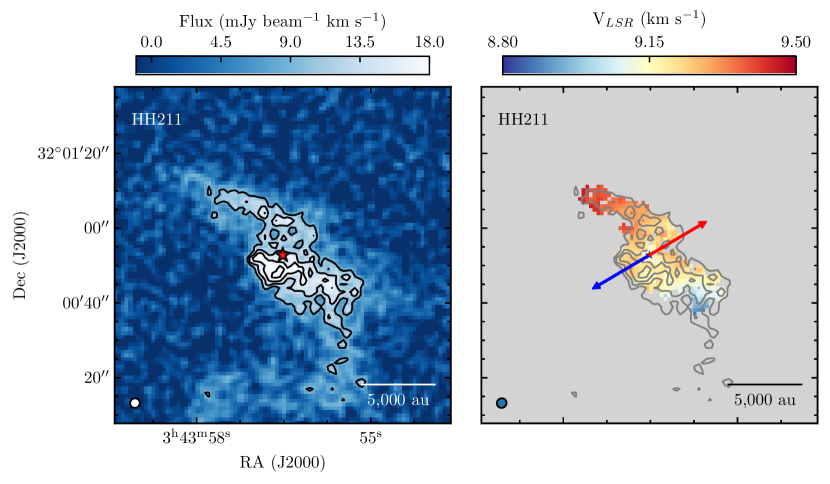
Figure 1: Left: Integrated intensity map of the $\textrm{NH}_{3}$ (1,1) line. Right: Velocity field for HH-211 derived from fitting the $\textrm{NH}_{3}$ (1,1) line. Outflow orientation is shown by the arrows. Contours are shown starting at 5$-\sigma$ with steps of 2$-\sigma$, where $\sigma=$1.9 mJy beam^-1 ${\rm km\,s^{-1}}$ is the standard deviation measured around the emission free region. Position of the protostar is shown by the star. Beam size and scale-bar are shown in the bottom-left and bottom-right corners, respectively.

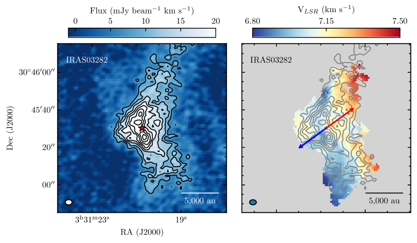
Figure 2: Like Fig.1, but for IRAS03282. The value of $\sigma$ is 1.6 mJy beam^-1 ${\rm km\,s^{-1}}$.

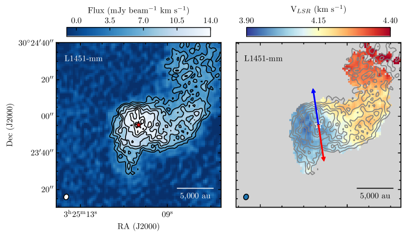
Figure 3: Like Fig.1, but for L1451-mm. The value of $\sigma$ is 0.9 mJy beam^-1 ${\rm km\,s^{-1}}$.

In the case of source HH211 and L1451-mm the centroid velocity maps show a clear velocity gradient in a direction perpendicular to the observed outflow. However, in the case of IRAS03282 the centroid velocity map also displays a velocity gradient along the outflow direction (Tobin et al., 2011), which creates a larger spread in the value of the specific angular momentum at any given rotation radius. Nevertheless, since the effect of the outflow appears to be present in both red and blue outflow components, then it is possible to derive the average rotational velocity, although with a larger uncertainty.

3.2 Specific angular momentum radial profile

The specific angular momentum at a distance $r$, is defined as $j(r)=r\times\delta v$, where $\delta v$ is the relative velocity of the gas with respect to the center of mass. In the case of symmetry around an axis, then the specific angular momentum can be described as, $j(r)=R_{rot}V_{rot}$, where $R_{rot}$ is the rotation radius in cylindrical coordinates (also called impact parameter) and $V_{rot}$ is the rotational velocity around its axis of symmetry. In this case, the derived $V_{rot}$ from the observations is similar to the brightness weighted centroid velocity, which corresponds to the mass weighted average velocity in simulations or theoretical calculations. Therefore, if we determine the rotational velocity at a given rotation radius then we can derive the specific angular momentum. A similar analysis was performed by Zhang et al. (2018) with numerical simulations, showing that the total specific angular momentum could be estimated. In the case of lines that are not very optically thick, the rotational velocity will correspond to the relative centroid velocity of the line along the line-of-sight ($V_{LSR}$) with respect of the core center (Tanner & Arce, 2010). A similar approach has been used to determine the velocity profile in disks (Murillo et al., 2013; Lindberg et al., 2014; Harsono et al., 2014, 2015). In the case of a protostellar core, we use the known YSO position and outflow orientation (see Table 2) to calculate the rotation radius. The YSO central velocity is estimated as the velocity of the dense gas, as probed using $\textrm{NH}_{3}$, at the position of the YSO. However, since we are not modelling the more complex dynamics involved closer to the disk scale (disk rotation and infall), then we discard all determinations of the specific angular momentum at distances smaller than the beam major axis.

Since the specific angular momentum should be close to constant for a given rotational radius, we determine the average value of the specific angular momentum at different rotational radii bins, and the associated uncertainty on the mean value. The results are shown in Fig. 4, with the radial profiles for all three sources, which appear almost indistinguishable. The radial profiles display a distribution consistent with a power-law (see Appendix B for the velocity comparison instead of the specific angular momentum). As a comparison, we also show the profile for a core with solid body rotation down to $5,000$ au, and conserved specific angular momentum within that radius using a dash line (Ohashi et al., 1997; Belloche, 2013), while also comparing to the best-fit to the high-angular resolution ALMA observations on L1527 that studied the inner envelope kinematics (Ohashi et al., 2014). The specific angular momentum derived of L1527 is substantially higher than the one measured here, which could be related to either a different initial condition or L1527 is a later evolutionary stage object (ambiguous due to the close to edge-on geometry) than those studied here.

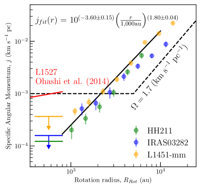
Figure 4: Radial profile of the specific angular momentum ($j=R_{rot}V_{rot}$) for the three sources studied: IRAS03282, HH211, and L1451-mm in blue, green, and yellow, respectively. Solid black line shows the best-fit power-law relation to the data between 800 and 10,000 au. The dash curve shows the previously proposed specific angular momentum profile (Ohashi et al., 1997; Belloche, 2013). The solid red line shows the best-fit power-law relation to the inner envelope of L1527 (Ohashi et al., 2014), which is a young protostar with a large disk.

The specific angular momentum profiles of the different sources are consistent with a single power-law. The resulting minimum least-squared power-law fit to all three sources is

$$j_{fit}(r)=10^{-3.60\pm 0.15}\left(\frac{r}{\textrm{1,000\,au}}\right)^{1.80\pm 0.04}\textrm{km\,s${}^{-1}$\,pc}~{}.$$ (1)

Notably, we do not find a break in the power-law down to 1,000 au, although there is a hint for a flattening on the radial profiles of IRAS03282 and L1451-mm. Higher resolution observations will be crucial to extend the radial profile down to smaller radii where the specific angular momentum could be conserved, and directly observe the flattening of the specific angular momentum profile.

4 Discussion

4.1 Interpretation of the power-law

The results are clear: the specific angular momentum radial profile is consistent with a single power-law down to 1,000 au. However, the power-law exponent is mid-way between the expected exponents for solid body rotation ($j\propto r^{2}$) and for turbulence ($j\propto r^{1.5}$) (Burkert & Bodenheimer, 2000).

For solid body rotation, the velocity at distance $r$ is $v(r)=\Omega r$, where $\Omega$ is the angular speed, and therefore the specific angular momentum is $j_{\rm SolidBody}=\Omega r^{2}$. In the case of a pure turbulent field that follows Larson’s relation ($\delta v(r)\propto r^{0.5}$), the dense cores kinematics (even at scales of $1,000$ au) might still be influenced by the turbulence of the parental molecular cloud/dense core.

This result suggests that dense cores do not present solid body rotation, as usually assumed. It might be an intermediate place in between turbulence dominated and solid body rotation. A similar exponent is also found in simulations of dense cores (Dib et al., 2010), once cores have evolved and are more gravitationally bound.

4.2 Are these results consistent with those for Dense cores?

The previous study of the total specific angular momentum, $J/M$, in dense cores by Goodman et al. (1993) found that

$$\frac{J}{M}=10^{-0.7\pm 0.2}\left(\frac{R}{\textrm{1\,pc}}\right)^{1.6\pm 0.2}~{},$$ (2)

where $J$ and $M$ are the total angular momentum and mass of the core, and solid body rotation and uniform density are assumed. This relation predicts a specific angular momentum at 1,000 au of $3.95\times 10^{-5}$ ${\rm km\,s^{-1}\,pc}$, which is only 16% below the directly measured values reported here.

We derived a more general expression for the total specific angular momentum (see Appendix C),

$$\frac{J}{M}(R)=\frac{(3-k_{p})}{2\,(3+k_{j}-k_{p})}j_{0}R^{k_{j}}\frac{\sqrt{\pi}\,\Gamma(k_{j}/2+1)}{\Gamma((k_{j}+3)/2)}~{},$$ (3)

where $\Gamma(x)$ is the Gamma function, under the assumption of a density profile $\rho\propto\rho_{0}r^{-k_{p}}$ and a specific angular momentum profile $j(r_{rot})=j_{0}r_{rot}^{k_{j}}$. This more general expression allow us to compare our results with those of Goodman et al. (1993).

The first thing to note is that if the specific angular momentum is described as a single power-law out to the dense core radius, then the exponent of the total specific angular momentum as a function of core radius is the same as the specific angular momentum profile (eqn. 3). Although the power-law exponents of these relations are slightly different, $1.8\pm 0.04$ compared to $1.6\pm 0.2$, they are consistent within the best fit uncertainties. We compare the derived total specific angular momentum for the entire core, $J/M(R)$, with the intrinsic specific angular momentum at the same scale, $j_{fit}(R)$, using eqn. 3. In the case of $k_{j}=1.8$ (the best fit value found here), and for typical density profiles ($k_{p}=0$, $1.5$, or $2$) the $J/M(R)$ is $0.43\,j(R)$, $0.31\,j(R)$ and $0.25\,j(R)$, respectively. Therefore, our results are within a factor of $1.5-3$ from those reported by Goodman et al. (1993).

4.3 Implications for largest Keplerian disk radius

Although we do not find the region with conserved specific angular momentum, if it is conserved from the 1,000 au scale down to the disk formation scales, then we can estimate the maximum possible Keplerian disk size using the relation

$$R_{disk}=\frac{j_{e}^{2}}{G\,M_{*}}~{},$$ (4)

see Yen et al. (2015), where $j_{e}$ is the specific angular momentum of the material that will form the disk, and $M_{*}$ is the stellar mass. This is a conservative upper limit to the Keplerian disk size, since we are not estimating the total enclosed mass only the stellar mass, and any other mechanism of angular momentum removal would reduce the infant disk radius.

We use our best fit to the angular momentum radial profile at 1,000 au, eq.(1), and estimate an upper limit to $j_{e}$ of $10^{-3.60}$ ${\rm km\,s^{-1}\,pc}$. In the case of a stellar mass of 0.05 M_⊙, which is appropriate for HH211 (Lee et al., 2009; Froebrich et al., 2003) and L1451-mm (Pineda et al., 2011; Maureira et al., 2017), we estimate an upper limit to the Keplerian disk radius of 60 au. This is consistent with disk radius estimates (including upper limits) for these sources using high-angular resolution dust continuum observations (see Table 2).

4.4 Estimating protostellar age

Some theoretical work relates the value of the constant specific angular momentum with the protostellar age (Takahashi et al., 2016). Again, we assume the specific angular momentum value at 1,000 au from the best fit, $j_{fit}(r)$ to estimate the collapse age of the core for these protostars using equation 26 from (Takahashi et al., 2016) of 11 kyr. This is consistent to the accretion age estimated for HH211 and L1451-mm of $(1-2)\times 10^{4}$ yr (Lee et al., 2009; Maureira et al., 2017). If this interpretation is correct, then it predicts that more evolved sources (e.g., Class I) would show a similar exponent but a variety of flattening radii depending on the source age, similar to the results from Yen et al. (2017) who assumed solid body rotation for the envelope.

4.5 Connecting with numerical simulations

Both the exponent and normalisation of the specific angular momentum profile derived from our observations are substantially different than those typically used as initial conditions for disk formation simulations (Ohashi et al., 1997; Belloche, 2013) or as a point of comparison for core properties in global simulations (Jappsen & Klessen, 2004; Ntormousi & Hennebelle, 2019; Kuznetsova et al., 2019). Here, we explore the implications for numerical simulations.

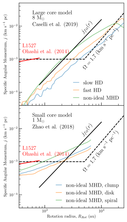
Figure 5: Specific angular momentum profile for the different sets of simulations in the large and small core models, top and bottom panels respectively. Our best fit to the data, $j_{fit}(r)$, is shown with a solid black line; the previously derived specific angular profile (Ohashi et al., 1997; Belloche, 2013) is shown with a dash black line; the power-law fit to the L1527 inner envelope kinematics (Ohashi et al., 2014) is shown with a red line. The non-ideal MHD simulation of the large prestellar core provides the best match to the observations of the Class 0 sources, while the non-ideal MHD simulations of a small protostellar core are closer to the observed kinematics of the (probably more evolved) L1527 source.

We use two sets of simulations already published in previous work (Zhao et al., 2018; Caselli et al., 2019) to explore the global trends of the specific angular momentum radial profile, but these simulations are not expected to be a perfect match to the presented data. The two simulations sets are split as large and small core models, and for each simulation we calculate the average specific angular momentum profiles for a given snapshot. The general descriptions of the simulations are the following:

(a)

The large core models correspond to a 8.1 $\textrm{M}_{\odot}$ dense core with a radius 50,000 au numerical simulations using HD and non-ideal magneto-hydro-dynamical (MHD) simulations showing the snapshot where the central density is 2$\times 10^{6}$ cm^-3, which are aimed at reproducing the properties of the L1544 prestellar core (more details in Caselli et al., 2019). Two HD simulations are run: “slow HD” and “fast HD” with angular speeds of 2.5$\times 10^{-14}$ s^-1 and 4$\times 10^{-14}$ s^-1, respectively, with the“fast HD” simulation rotating close to the maximum speed that would allow collapse ($\Omega_{max}$=6$\times 10^{-14}$ s^-1 in the case of $\beta$=0.5 and solid body rotation). The MHD simulation is run with angular speed of 4$\times 10^{-14}$ s^-1, magnetic field of $B_{0}$=14.8 $\mu$G, and a mass-to-flux ratio $\lambda$ of $\sim$1.

(b)

The small core models correspond to a 1 $\textrm{M}_{\odot}$ dense core with a 6,666 au radius, using non-ideal MHD simulations with different angular speed rotation and magnetic field strength as initial conditions (more details in Zhao et al., 2018). Here we consider the snapshot where the star and disk total mass is $\sim$0.1 $\textrm{M}_{\odot}$, aimed at reproducing protostellar systems in the early stages of evolution (close to Class 0). The “disk” and “spiral” simulations have a magnetic field of 42.5 $\mu$G ($\lambda\sim 2.4$), while the “clump” simulation has a magnetic field of 21.3 $\mu$G ($\lambda\sim 4.8$). The “disk” and “clump” simulations have an angular speed of $10^{-13}$ s^-1, while the “spiral” simulation has an angular speed of $2\times 10^{-13}$ s^-1.

Figure 5 compares the best fit to the data and the profiles from the simulations. Top panel of Figure 5 shows the profiles for the large core model that has not formed a protostar yet, in which the non-ideal MHD simulation presents a smoother profile and with a slope and amplitude in the inner 4,000 au which is much closer to the best fit to observations than the HD simulations. The main reason for this increased specific angular momentum in the non-ideal MHD simulation compared to the HD ones, is that the collapse takes longer in the non-ideal MHD case to reach the same central density. This keeps the angular momentum in the outer parts fo the dense core for a longer period of time, which generates an increased specific angular momentum at intermediate scales (700 – 4,000 au). The bottom panel of Figure 5 shows the profiles for the small core model that already formed a disk, which are much flatter than our best fit from observations. However, all these models are consistent with the result for L1527 shown with a red line (Ohashi et al., 2014), since each simulation will evolve with time in such a way that the radial profile does not change the slope, but it does change the normalisation. These results suggests that the Class 0 sources here observed are indeed very young, and their dense core kinematics might still resemble that of the parental dense core. On the other hand, the kinematics of the (possibly more evolved) L1527 is better reproduced by simulations which already formed a protostar and disk system. This highlights the need to properly determine the probable evolution of the specific angular momentum as a function of source evolutionary stage.

5 Summary and Conclusions

We analysed VLA $\textrm{NH}_{3}$ (1,1) data for 3 of the youngest protostellar sources in the Perseus molecular cloud to determine the dense gas kinematics of the material involved in the disk formation process. Our main results are summarised below.

• We determine the specific angular momentum radial profile for three YSOs and find that is consistent among these three sources:

  $$j(r)=10^{-3.60\pm 0.15}\left(\frac{r}{1,000\textrm{\,au}}\right)^{1.80\pm 0.04}~{}{{\rm km\,s^{-1}\,pc}}~{},$$

  and find that the region of conserved specific angular momentum must be smaller than 1,000 au radius.

• We determine expressions for the specific angular momentum of the entire core under a more general condition, $j(r)\propto r_{rot}^{k_{j}}$, than solid body rotation.

• The specific angular momentum radial profile normalisation is consistent with previous determinations of the total specific angular momentum based on dense core solid body rotation fits, but only after we correct for the non-solid body rotation nature of the cores.

• If the specific angular momentum is conserved inwards of 1,000 au, then the largest disk towards these low-mass YSOs ($M_{*}\sim$0.05 $\textrm{M}_{\odot}$) is 60 au in radius, which is consistent with previous high-angular resolution studies focused on the disk properties.

• We compare to already published numerical simulations for a large prestellar dense core and a small protostellar dense core. The comparison shows that the non-ideal MHD simulation of a prestellar core provides a good match to the observed profile, and better than HD simulations. The protostellar simulations show profiles more similar to that of L1527. This suggests a magnetic field regulated dynamical evolution between pre-stellar and protostellar cores.

These results show the potential for constraining the disk formation process by connecting to the knowledge of the parental dense core properties. Future observations might reveal possible variations with environment and evolution on the specific angular momentum profile.

Appendix A Velocity dispersion maps

The velocity dispersion maps (without removal of channel width response) for all three sources are shown in Figure 6. As reported in previously, these velocity dispersions correspond to non-thermal velocity dispersions below the sonic sound speed (Mach number $<0.5$), but with an increase towards to the protostar position, which is most likely due to protostellar feedback.

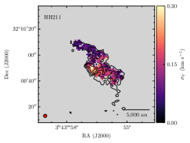
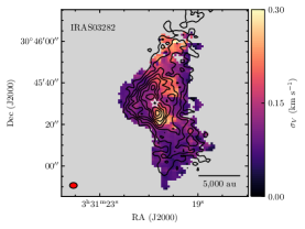
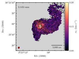
Figure 6: Velocity dispersion maps for all three sources: HH-211, IRAS03282, and L1451-mm in the left, middle, and right panels, respectively. Beam size and scale bar are shown in bottom left and right corners, respectively.

Appendix B Rotational velocity as a function of radius

A reasonable concern is that the calculation of $j(r)=R_{rot}\,V_{rot}$ could be mostly driven by $R_{rot}$, instead of a real radial dependence. A direct check for this possible issue is done by comparing the average velocity as a function of radius, using the same radial bins as the average specific angular momentum as a function of radius. Notice, that for this calculation we use the actual relative velocity derived from the data. We compare the results for all three sources in Fig. 7 against the predicted rotational velocity as a function of radius for the specific angular momentum best fit and for the proposed profile by Ohashi et al. (1997) and Belloche (2013). The data are better described by a single power-law, without evidence for a transition to a conserved angular momentum regime, as previously proposed. This comparison confirms our results from fitting the specific angular momentum.

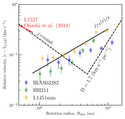
Figure 7: Rotational velocity as a function of radius for all three sources observed, measured using the relative velocity measurement. Similar to Fig. 4, the black solid line is the expected rotational velocity derived from the specific angular momentum best fit, $V_{fit}(r)=j_{fit}(r)/r$, while the proposed rotational velocity profile by Ohashi et al. (1997) and Belloche (2013) is shown by the dashed line. The data show a clear correlation with radius which is well described by $V_{fit}(r)$, while the dashed line profile poorly describes the data. The best fit rotational velocity profile derived for L1527 IRS by Ohashi et al. (2014) is shown by the red line.

Appendix C Properties as function of radius

Here we show how to determine the total angular momentum ($J$) and specific angular momentum ($J/M$) in the case of differential rotation and/or a radial density profile.

Assuming that the density profile is spherically symmetric and that it can be described by a single power-law, depending only on the distance to the central protostar:

$$\rho=\rho_{0}r^{-k_{p}}~{}.$$ (C1)

Naturally, the total enclosed mass can be described as

$$M(<R)=\frac{4\pi}{(3-k_{p})}\rho_{0}R^{3-k_{p}}~{},$$ (C2)

for $k_{p}\neq 3$.

Also, assuming that the specific angular momentum can be described in spherical coordinates as

$$j(r,\theta)=j_{0}(r\sin\theta)^{k_{j}}~{},$$ (C3)

where $k_{j}=2$ represents solid body rotation, the total angular momentum within a radius $R$ is

$$J(R) = \int_{Volume}j(r,\theta)\rho(r)d\Omega r^{2}dr$$ (C4)

$$= \int_{0}^{2\pi}\int_{0}^{\pi}\int_{0}^{R}j_{0}(r\sin\theta)^{k_{j}}\,\rho_{0}r^{-k_{p}}\,\sin\theta r^{2}\,drd\theta d\phi$$

$$= 2\pi\int_{0}^{\pi}\sin^{k_{j}+1}\theta d\theta\int_{0}^{R}\rho_{0}j_{0}r^{2+k_{j}-k_{p}}\,dr$$

$$= \frac{2\pi}{(3+k_{j}-k_{p})}\rho_{0}j_{0}R^{(3+k_{j}-k_{p})}\int_{0}^{\pi}\sin^{k_{j}+1}\theta d\theta~{},$$ (C6)

for $(k_{p}-k_{j})\neq 3$.

The total specific angular momentum can be written as

$$\frac{J}{M}(R)=\frac{(3-k_{p})}{2(3+k_{j}-k_{p})}j_{0}R^{k_{j}}\int_{0}^{\pi}\sin^{k_{j}+1}\theta d\theta~{}.$$ (C7)

The defined integral can be written as

$$\int_{0}^{\pi}\sin^{\alpha+1}xdx = \frac{\sqrt{\pi}\,\Gamma(\alpha/2+1)}{\Gamma((\alpha+3)/2)}$$ (C8)

for $\alpha>-2$, and where $\Gamma(x)$ is the Gamma function. Therefore,

$$\frac{J}{M}(R)=\frac{(3-k_{p})}{2\,(3+k_{j}-k_{p})}j_{0}R^{k_{j}}\frac{\sqrt{\pi}\,\Gamma(k_{j}/2+1)}{\Gamma((k_{j}+3)/2)}~{},$$ (C9)

equivalent to equation 3.

The rotational energy is calculated as,

$$E_{rot}(R) = \int\frac{1}{2}v_{rot}(r,\theta)^{2}\rho(r)dV$$

$$= \pi\int\left(j_{0}(r\sin\theta)^{k_{j}-1}\right)^{2}\rho_{0}r^{-k_{p}}\sin\theta r^{2}drd\theta$$

$$= \pi\int j_{0}^{2}(r\sin\theta)^{2\,k_{j}-2}\rho_{0}r^{2-k_{p}}\sin\theta drd\theta$$

$$= \pi\rho_{0}j_{0}^{2}\int_{0}^{R}r^{2k_{j}-k_{p}}dr\int_{0}^{\pi}\sin^{2\,k_{j}-1}\theta d\theta$$

$$= \frac{\pi\rho_{0}j_{0}^{2}}{(2k_{j}-k_{p}+1)}R^{2k_{j}-k_{p}+1}\int_{0}^{\pi}\sin^{2k_{j}-1}\theta d\theta$$

$$= \frac{\pi\rho_{0}j_{0}^{2}}{(2k_{j}-k_{p}+1)}R^{2k_{j}-k_{p}+1}\frac{\sqrt{\pi}\,\Gamma(k_{j})}{\Gamma(k_{j}+1/2)}$$

$$= \frac{(3-k_{p})}{(2k_{j}-k_{p}+1)}\frac{MR^{2(k_{j}-1)}j_{0}^{2}}{4}\frac{\sqrt{\pi}\,\Gamma(k_{j})}{\Gamma(k_{j}+1/2)}~{}.$$ (C11)

The total gravitational energy is

$$U = -\frac{(4\pi\rho_{0})^{2}G}{(3-k_{p})(5-2k_{p})}R^{5-2k_{p}}$$ (C12)

$$= -\frac{(3-k_{p})}{(5-2k_{p})}\frac{GM^{2}}{R}~{}.$$ (C13)

The ratio of the rotational and gravitation energy, $\beta=E_{rot}/|U|$, is

$$\beta = \frac{j_{0}^{2}}{(2k_{j}-k_{p}+1)}R^{2k_{j}+k_{p}-4}\frac{(3-k_{p})(5-2k_{p})}{16\pi\rho_{0}G}\frac{\sqrt{\pi}\,\Gamma(k_{j})}{\Gamma(k_{j}+1/2)}$$ (C14)

$$= \frac{(3-k_{p})}{(2k_{j}-k_{p}+1)}\frac{MR^{2(k_{j}-1)}j_{0}^{2}}{4}\frac{\sqrt{\pi}\,\Gamma(k_{j})}{\Gamma(k_{j}+1/2)}\frac{(4\pi\rho_{0})^{2}G}{(3-k_{p})(5-2k_{p})}R^{5-2k_{p}}$$ (C15)

$$= \frac{(5-2k_{p})}{(2k_{j}-k_{p}+1)}\frac{R^{2k_{j}-1}j_{0}^{2}}{4GM}\frac{\sqrt{\pi}\,\Gamma(k_{j})}{\Gamma(k_{j}+1/2)}~{}.$$ (C16)

References

- Allen et al. (2003) Allen, A., Li, Z.-Y., & Shu, F. H. 2003, ApJ, 599, 363. http://dx.doi.org/10.1086/379243
- Belloche (2013) Belloche, A. 2013, EAS Publications Series, 62, 25. http://dx.doi.org/10.1051/eas/1362002
- Benson & Myers (1989) Benson, P. J., & Myers, P. C. 1989, ApJS, 71, 89. http://dx.doi.org/10.1086/191365
- Burkert & Bodenheimer (2000) Burkert, A., & Bodenheimer, P. 2000, ApJ, 543, 822. http://dx.doi.org/10.1086/317122
- Caselli et al. (2002) Caselli, P., Benson, P. J., Myers, P. C., & Tafalla, M. 2002, ApJ, 572, 238. http://dx.doi.org/10.1086/340195
- Caselli et al. (2019) Caselli, P., Pineda, J. E., Zhao, B., et al. 2019, ApJ, 874, 89
- Chen et al. (2007) Chen, X., Launhardt, R., & Henning, T. 2007, ApJ, 669, 1058
- Crapsi et al. (2007) Crapsi, A., Caselli, P., Walmsley, M. C., & Tafalla, M. 2007, A&A, 470, 221
- Dib et al. (2010) Dib, S., Hennebelle, P., Pineda, J. E., et al. 2010, ApJ, 723, 425. http://dx.doi.org/10.1088/0004-637X/723/1/425
- Dunham et al. (2014) Dunham, M. M., Vorobyov, E. I., & Arce, H. G. 2014, Monthly Notices of the Royal Astronomical Society, 444, 887. http://dx.doi.org/10.1093/mnras/stu1511
- Enoch et al. (2011) Enoch, M. L., Corder, S., Duchêne, G., et al. 2011, ApJS, 195, 21. http://dx.doi.org/10.1088/0067-0049/195/2/21
- Friesen et al. (2017) Friesen, R. K., Pineda, J. E., co-PIs, et al. 2017, ApJ, 843, 63
- Froebrich et al. (2003) Froebrich, D., Smith, M. D., Hodapp, K.-W., & Eisloffel, J. 2003, Monthly Notices of the Royal Astronomical Society, 346, 163. http://dx.doi.org/10.1046/j.1365-2966.2003.07072.x
- Ginsburg & Mirocha (2011) Ginsburg, A., & Mirocha, J. 2011, PySpecKit: Python Spectroscopic Toolkit, Astrophysics Source Code Library, , , ascl:1109.001
- Goodman et al. (1998) Goodman, A. A., Barranco, J. A., Wilner, D. J., & Heyer, M. H. 1998, ApJ, 504, 223. http://dx.doi.org/10.1086/306045
- Goodman et al. (1993) Goodman, A. A., Benson, P. J., Fuller, G. A., & Myers, P. C. 1993, ApJ, 406, 528. http://dx.doi.org/10.1086/172465
- Harsono et al. (2014) Harsono, D., Jørgensen, J. K., van Dishoeck, E. F., et al. 2014, Astronomy & Astrophysics, 562, A77. http://dx.doi.org/10.1051/0004-6361/201322646
- Harsono et al. (2015) Harsono, D., van Dishoeck, E. F., Bruderer, S., Li, Z.-Y., & Jørgensen, J. K. 2015, Astronomy & Astrophysics, 577, A22. http://dx.doi.org/10.1051/0004-6361/201424550
- Hennebelle & Teyssier (2008) Hennebelle, P., & Teyssier, R. 2008, A&A, 477, 25
- Hunter (2007) Hunter, J. D. 2007, Computing In Science & Engineering, 9, 90
- Jappsen & Klessen (2004) Jappsen, A.-K., & Klessen, R. S. 2004, A&A, 423, 1
- Joos et al. (2012) Joos, M., Hennebelle, P., & Ciardi, A. 2012, A&A, 543, A128
- Jørgensen et al. (2009) Jørgensen, J. K., van Dishoeck, E. F., Visser, R., et al. 2009, Astronomy and Astrophysics, 507, 861. http://dx.doi.org/10.1051/0004-6361/200912325
- Kurono et al. (2013) Kurono, Y., Saito, M., Kamazaki, T., Morita, K.-I., & Kawabe, R. 2013, ApJ, 765, 85
- Kuznetsova et al. (2019) Kuznetsova, A., Hartmann, L., & Heitsch, F. 2019, ApJ, 876, 33
- Lee et al. (2009) Lee, C.-F., Hirano, N., Palau, A., et al. 2009, ApJ, 699, 1584. http://dx.doi.org/10.1088/0004-637X/699/2/1584
- Lee et al. (2018) Lee, C.-F., Li, Z.-Y., Hirano, N., et al. 2018, ApJ, 863, 94
- Lee et al. (2019) Lee, C.-F., Kwon, W., Jhan, K.-S., et al. 2019, arXiv e-prints, arXiv:1905.09417
- Li et al. (2014) Li, Z.-Y., Krasnopolsky, R., Shang, H., & Zhao, B. 2014, ApJ, 793, 130
- Lindberg et al. (2014) Lindberg, J. E., Jørgensen, J. K., Brinch, C., et al. 2014, A&A, 566, A74
- Maureira et al. (2017) Maureira, M. J., Arce, H. G., Dunham, M. M., et al. 2017, ApJ, 838, 60
- Maury et al. (2010) Maury, A. J., André, P., Hennebelle, P., et al. 2010, Astronomy and Astrophysics, 512, A40. http://dx.doi.org/10.1051/0004-6361/200913492
- Maury et al. (2019) Maury, A. J., André, P., Testi, L., et al. 2019, A&A, 621, A76
- McMullin et al. (2007) McMullin, J. P., Waters, B., Schiebel, D., Young, W., & Golap, K. 2007, in Astronomical Society of the Pacific Conference Series, Vol. 376, Astronomical Data Analysis Software and Systems XVI, ed. R. A. Shaw, F. Hill, & D. J. Bell, 127
- Mellon & Li (2008) Mellon, R. R., & Li, Z.-Y. 2008, ApJ, 681, 1356. http://dx.doi.org/10.1086/587542
- Murillo et al. (2013) Murillo, N. M., Lai, S.-P., Bruderer, S., Harsono, D., & van Dishoeck, E. F. 2013, Astronomy & Astrophysics, 560, A103. http://dx.doi.org/10.1051/0004-6361/201322537
- Ntormousi & Hennebelle (2019) Ntormousi, E., & Hennebelle, P. 2019, A&A, 625, A82
- Ohashi et al. (1997) Ohashi, N., Hayashi, M., Ho, P. T. P., et al. 1997, ApJ, 488, 317
- Ohashi et al. (2014) Ohashi, N., Saigo, K., Aso, Y., et al. 2014, ApJ, 796, 131. http://dx.doi.org/10.1088/0004-637X/796/2/131
- Ortiz-León et al. (2018) Ortiz-León, G. N., Loinard, L., Dzib, S. A., et al. 2018, ApJ, 865, 73
- Pineda et al. (2010) Pineda, J. E., Goodman, A. A., Arce, H. G., et al. 2010, ApJ, 712, L116. http://dx.doi.org/10.1088/2041-8205/712/1/L116
- Pineda et al. (2011) Pineda, J. E., Arce, H. G., Schnee, S., et al. 2011, ApJ, 743, 201. http://dx.doi.org/10.1088/0004-637X/743/2/201
- Pineda et al. (2015) Pineda, J. E., Offner, S. S. R., Parker, R. J., et al. 2015, Nature, 518, 213
- Robitaille & Bressert (2012) Robitaille, T., & Bressert, E. 2012, APLpy: Astronomical Plotting Library in Python, , , ascl:1208.017
- Rosolowsky et al. (2008) Rosolowsky, E. W., Pineda, J. E., Foster, J. B., et al. 2008, The Astrophysical Journal Supplement Series, 175, 509. http://dx.doi.org/10.1086/524299
- Segura-Cox et al. (2018) Segura-Cox, D. M., Looney, L. W., Tobin, J. J., et al. 2018, ApJ, 866, 161
- Seifried et al. (2011) Seifried, D., Banerjee, R., Klessen, R. S., Duffin, D., & Pudritz, R. E. 2011, Monthly Notices of the Royal Astronomical Society, 417, 1054. http://dx.doi.org/10.1111/j.1365-2966.2011.19320.x
- Seifried et al. (2012) Seifried, D., Banerjee, R., Pudritz, R. E., & Klessen, R. S. 2012, Monthly Notices of the Royal Astronomical Society: Letters, 423, L40. http://dx.doi.org/10.1111/j.1745-3933.2012.01253.x
- Tafalla et al. (2004) Tafalla, M., Myers, P. C., Caselli, P., & Walmsley, C. M. 2004, Astronomy and Astrophysics, 416, 191. http://dx.doi.org/10.1051/0004-6361:20031704
- Takahashi et al. (2016) Takahashi, S. Z., Tomida, K., Machida, M. N., & Inutsuka, S.-i. 2016, MNRAS, 463, 1390
- Tanner & Arce (2010) Tanner, J. D., & Arce, H. G. 2010, ApJ, 726, 40. http://dx.doi.org/10.1088/0004-637X/726/1/40
- Tatematsu et al. (2016) Tatematsu, K., Ohashi, S., Sanhueza, P., et al. 2016, Publ. Astron. Soc. Jpn, 68, 24. http://dx.doi.org/10.1093/pasj/psw002
- Tobin et al. (2012) Tobin, J. J., Hartmann, L., Bergin, E., et al. 2012, ApJ, 748, 16
- Tobin et al. (2011) Tobin, J. J., Hartmann, L., Chiang, H.-F., et al. 2011, ApJ, 740, 45. http://dx.doi.org/10.1088/0004-637X/740/1/45
- Tobin et al. (2016) Tobin, J. J., Looney, L. W., Li, Z.-Y., et al. 2016, ApJ, 818, 73
- Tomida et al. (2015) Tomida, K., Okuzumi, S., & Machida, M. N. 2015, ApJ, 801, 117
- Tomida et al. (2013) Tomida, K., Tomisaka, K., Matsumoto, T., et al. 2013, ApJ, 763, 6
- Yen et al. (2015) Yen, H.-W., Koch, P. M., Takakuwa, S., et al. 2015, ApJ, 799, 193. http://dx.doi.org/10.1088/0004-637X/799/2/193
- Yen et al. (2017) Yen, H.-W., Koch, P. M., Takakuwa, S., et al. 2017, ApJ, 834, 178
- Yen et al. (2015) Yen, H.-W., Takakuwa, S., Koch, P. M., et al. 2015, ApJ, 812, 129
- Zhang et al. (2018) Zhang, S., Hartmann, L., Zamora-Avilés, M., & Kuznetsova, A. 2018, MNRAS, 480, 5495
- Zhao et al. (2018) Zhao, B., Caselli, P., Li, Z.-Y., & Krasnopolsky, R. 2018, MNRAS, 473, 4868
- Zhao et al. (2016) Zhao, B., Caselli, P., Li, Z.-Y., et al. 2016, MNRAS, 460, 2050
- Zucker et al. (2018) Zucker, C., Schlafly, E. F., Speagle, J. S., et al. 2018, ApJ, 869, 83