Lattice Transformer for Speech Translation

Abstract

Recent advances in sequence modeling have highlighted the strengths of the transformer architecture, especially in achieving state-of-the-art machine translation results. However, depending on the up-stream systems, e.g., speech recognition, or word segmentation, the input to translation system can vary greatly. The goal of this work is to extend the attention mechanism of the transformer to naturally consume the lattice in addition to the traditional sequential input. We first propose a general lattice transformer for speech translation where the input is the output of the automatic speech recognition (ASR) which contains multiple paths and posterior scores. To leverage the extra information from the lattice structure, we develop a novel controllable lattice attention mechanism to obtain latent representations. On the LDC Spanish-English speech translation corpus, our experiments show that lattice transformer generalizes significantly better and outperforms both a transformer baseline and a lattice LSTM. Additionally, we validate our approach on the WMT 2017 Chinese-English translation task with lattice inputs from different BPE segmentations. In this task, we also observe the improvements over strong baselines.

1 Introduction

Transformer based encoder-decoder framework Vaswani et al. (2017) for Neural Machine Translation (NMT) has currently become the state-of-the-art in many translation tasks, significantly improving translation quality in text Bojar et al. (2018); Fan et al. (2018) as well as in speech Jan et al. (2018). Most NMT systems fall into the category of Sequence-to-Sequence (Seq2Seq) model Sutskever et al. (2014), because both the input and output consist of sequential tokens. Therefore, in most neural speech translation, such as that of Bojar et al. (2018), the input to the translation system is usually the 1-best hypothesis from the ASR instead of the word lattice output with its corresponding probability scores.

How to consume word lattice rather than sequential input has been substantially researched in several natural language processing (NLP) tasks, such as language modeling Buckman and Neubig (2018), Chinese Named Entity Recognition (NER) Zhang and Yang (2018), and NMT Su et al. (2017). Additionally, some pioneering works Adams et al. (2016); Sperber et al. (2017); Osamura et al. (2018) demonstrated the potential improvements in speech translation by leveraging the additional information and uncertainty of the packed lattice structure produced by ASR acoustic model.

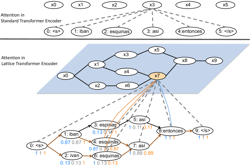
Figure 1: Illustration of our proposed attention mechanism (best viewed in color). Our attention depends on the tokens of common paths and forward (blue) / marginal (grey) / backward (orange) probability scores.

Efforts have since continued to push the boundaries of long short-term memory (LSTM) Hochreiter and Schmidhuber (1997) models. More precisely, most previous works are in line with the existing method Tree-LSTMs Tai et al. (2015), adapting to task-specific variant Lattice-LSTMs that can successfully handle lattices and robustly establish better performance than the original models. However, the inherently sequential nature still remains in Lattice-LSTMs due to the topological representation of the lattice graph, precluding long-path dependencies Khandelwal et al. (2018) and parallelization within training examples that are the fundamental constraint of LSTMs.

In this work, we introduce a generalization of the standard transformer architecture to accept lattice-structured network topologies. The standard transformer is a transduction model relying entirely on attention modules to compute latent representations, e.g., the self-attention requires to calculate the intra-attention of every two tokens for each sequence example. Latest works such as Yu et al. (2018); Devlin et al. (2018); Lample et al. (2018); Su et al. (2018) empirically find that transformer can outperform LSTMs by a large margin, and the success is mainly attributed to self-attention. In our lattice transformer, we propose a lattice relative positional attention mechanism that can incorporate the probability scores of ASR word lattices. The major difference with the self-attention in transformer encoder is illustrated in Figure 1.

We first borrow the idea from the relative positional embedding Shaw et al. (2018) to maximally encode the information of the lattice graph into its corresponding relative positional matrix. This design essentially does not allow a token to pay attention to any token that has not appeared in a shared path. Secondly, the attention weights depend not only on the query and key representations in the standard attention module, but also on the marginal / forward / backward probability scores Rabiner (1989); Post et al. (2013) derived from the upstream systems (such as ASR). Instead of 1-best hypothesis alone (though it is based on forward scores), the additional probability scores have rich information about the distribution of each path Sperber et al. (2017). It is in principle possible to use them, for example in attention weights reweighing, to increase the uncertainty of the attention for other alternative tokens.

Our lattice attention is controllable and flexible enough for the utilization of each score. The lattice transformer can readily consume the lattice input alone if the scores are unavailable. A common application is found in the Chinese NER task, in which a Chinese sentence could possibly have multiple word segmentation possibilities Zhang and Yang (2018). Furthermore, different BPE operations Sennrich et al. (2016) or probabilistic subwords Kudo (2018) can also bring similar uncertainty to subword candidates and form a compact lattice structure.

In summary, this paper makes the following main contributions. i) To our best knowledge, we are the first to propose a novel attention mechanism that consumes a word lattice and the probability scores from the ASR system. ii) The proposed approach is naturally applied to both the encoder self-attention and encoder-decoder attention. iii) Another appealing feature is that the lattice transformer can be reduced to standard lattice-to-sequence model without probability scores, fitting the text translation task. iv) Extensive experiments on speech translation datasets demonstrate that our method outperforms the previous transformer and Lattice-LSTMs. The experiment on the WMT 2017 Chinese-English translation task shows the reduced model can improve many strong baselines such as the transformer.

2 Background

We first briefly describe the standard transformer that our model is built upon, and then elaborate on our proposed approach in the next section.

2.1 Transformer

The Transformer follows the typical encoder-decoder architecture using stacked self-attention, point-wise fully connected layers, and the encoder-decoder attention layers. Each layer is in principle wrapped by a residual connection He et al. (2016) and a postprocessing layer normalization Ba et al. (2016). Although in principle, it is not necessary to mask for self-attentions in the encoder, in practical implementation it is required to mask the padding positions. However, self-attention in the decoder only allows positions up to the current one to be attended to, preventing information flow from the left and preserving the auto-regressive property. The illegal connections will be masked out by setting as $-10^{9}$ before the softmax operation.

2.2 Dot-product Attention

Suppose that for each attention layer in the transformer encoder and decoder, we have two input sequences that can be presented as two matrices $X\in\mathcal{R}^{n\times d}$ and $Y\in\mathcal{R}^{m\times d}$, where $n,m$ are the lengths of source and target sentences respectively, and $d$ is the hidden size (usually equal to embedding size), the output is $h$ new sequences $Z_{i}\in\mathcal{R}^{n\times d/h}$ or $\in\mathcal{R}^{m\times d/h}$, where $h$ is the number of heads in attention. In general, the result of multi-head attention is calculated according to the following procedure.

$$Q =XW^{Q}\text{ or }YW^{Q}\text{ or }YW^{Q}$$ (1)

$$K =XW^{K}\text{ or }YW^{K}\text{ or }XW^{K}$$ (2)

$$V =XW^{V}\text{ or }YW^{V}\text{ or }XW^{V}$$ (3)

$$Z_{i} =\textbf{Softmax}\left(\frac{QK^{\top}}{\sqrt{d/h}}+\mathbb{I}_{d}M\right)V$$ (4)

$$Z =\textbf{Concat}(Z_{1},...,Z_{h})W^{O}$$ (5)

where the matrices $W^{Q},W^{K},W^{V}\in\mathcal{R}^{d\times d/h}$ and $W^{O}\in\mathcal{R}^{d\times d}$ represent the learnable projection parameters, and the masking matrix $M\in\mathcal{R}^{m\times m}$ is an upper triangular matrix with zero on the diagonal and non-zero ($-10^{9}$) everywhere else.

Note that i) the three columns in the right-side of Eq (1,2,3) are used to compute the encoder self-attention, the decoder self-attention, and the encoder-decoder attention respectively, ii) $\mathbb{I}_{d}$ is the indicator function that returns 1 if it computes decoder self-attention and 0 otherwise, iii) the projection parameters are unique per layer and head, iv) the Softmax in Eq (4) means a row-wise matrix operation, computing the attention weights by scaled dot product and resulting in a simplex $\Delta^{n}$ for each row.

3 Lattice Transformer

As motivated in the introduction, our goal is to enhance the standard transformer architecture, which is limited to sequential inputs, to consume lattice inputs with additional information from the up-stream ASR systems.

3.1 Lattice Representation

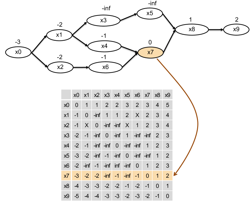
Figure 2: An example of the lattice relative position matrix, where “-inf” in the matrix is a special number denoting that no relative position exists between the corresponding two tokens.

Without loss of generality, we assume a word lattice from ASR system to be a directed, connected and acyclic graph following a topological ordering such that a child node comes after its parent nodes. We add two special tokens to each path of the lattice, which represent the start of sentence and the end of sentence (e.g., Figure 1), so that the graph has a single source node and a single end node, where each node is assigned a token.

Given the definition and property described above, we propose to use a relative positional lattice matrix $L\in\mathcal{N}^{n\times n}$ to encode the graph information, where $n$ is number of nodes in the graph. For any two nodes $i,j$ in the lattice graph, the matrix entry $L_{ij}$ is the minimum relative distance between them. In other words, if the nodes $i,j$ share at least one path, then we have

$$L_{ij}=\min_{p\in\text{common paths for $i,j$}}L_{i0}^{p}-L_{j0}^{p},$$ (6)

where $L_{\cdot 0}^{p}$ is the distance to the source node in path $p$. If no common path exists for two nodes, we denote the relative distance as $-\infty$ ($-10^{9}$ in practice) for subsequent masking in the lattice attention. The reason for choosing the “$\min$” in Eq (6) is that in our dataset we find about 70% of $L_{ij}$s computed by “$\min$” and “$\max$” are identical, and about 20% entries just differ by 1. Empirically, our experiments also show no significant difference in the performance of either one.

An illustration to compute the lattice matrix for the example in the introduction is shown in Figure 2. Since we can deterministically reconstruct the lattice graph from those matrix elements that are equal to 1, it indicates the relation information between the parent and child nodes.

3.2 Controllable Lattice Attention

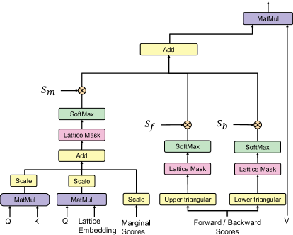
Figure 3: Left panel: the controllable lattice attention, where $s_{m},s_{f},s_{b}$ are learnable scalars and $s_{m}+s_{f}+s_{b}=1$. Right panel: the overall model architecture of lattice transformer.

Besides the lattice graph representation, the posterior probability scores can be simultaneously produced from the acoustic model and language model in most ASR systems. We deliberately design a controllable lattice attention mechanism to incorporate such information to make the attention encode more uncertainties.

In general, we denote the posterior probability of a node $i$ as the forward score $f_{i}$, where the summation of the forward scores for its child nodes is 1. Following the recursion rule in Rabiner (1989), we can further derive another two useful probabilities, the marginal score $m_{i}=f_{i}\sum_{j\in\text{Pa}(i)}m_{j}$ and the backward score $b_{i}=m_{i}/\sum_{k\in\text{Ch}(i)}m_{k}$, where $\text{Pa}(i)$ or $\text{Ch}(i)$ denotes node $i$’s predecessor or successor set, respectively. Intuitively, the marginal score measures the global importance of the current token compared with its substitutes given all predecessors; the backward score is analogous to the forward score, which is only locally associated with the importance of different parents to their children, where the summation of its parent nodes’ scores is 1. Therefore, our controllable attention aims to employ marginal scores and forward / backward scores.

3.2.1 Lattice Embedding

We first construct the latent representations of the relative positional lattice matrix $L$. The matrix $L$ can be straightforwardly decomposed into two matrices: one is the mask $L^{M}$ with only 0 and $-\infty$ values, and the other is the matrix with regular values i.e., $L^{R}=L-L^{M}$. Given a 2D embedding matrix $W^{L}$, the embedded vector of $L^{R}_{ij}$ can be written as $W^{L}[L^{R}_{ij},:]$ with the NumPy style indexing. In order to prevent the the lattice embedding from dynamically changing, we have to clip every entry of $L^{R}$ with a positive integer $c$, such that $W^{L}\in\mathcal{R}^{(2c+1)\times d/h}$ has a fixed dimensionality and becomes learnable parameters.

3.2.2 Attention with Probability Scores

Our proposed controllable lattice attention is depicted in the left panel of Figure 3. It shows the computational graph with detailed network modules. More concretely, we first denote the lattice embedding for $L^{R}$ as a 3D array $E\in\mathcal{R}^{n\times n\times d/h}$. Then, the attention weights adapted from traditional transformer are integrated with marginal scores that capture the distribution of each path in the lattice. The logits in Eq (4) will become the addition of three individual terms (if we temporarily omit the mask matrix),

$$\frac{QK^{\top}+\textbf{einsum}(\texttt{'ik,ijk->ij'},Q,E)}{\sqrt{d/h}}$$

$$+w_{m}\mathbf{m}~{}.$$ (7)

The original $QK^{\top}$ will remain since the word embeddings have the majority of significant semantic information. The difficult part in Eq (7) is the new dot product term involving the lattice embedding by einsum operation, where einsum is a multi-dimensional linear algebraic array operation in Einstein summation convention. In our case, it tries to sum out the dimension of the hidden size, resulting in a new 2D array $\in\mathcal{R}^{n\times n}$, which is further be scaled by $\frac{1}{\sqrt{d/h}}$ as well. In addition, we aggregate the scaled marginal score vector $\mathbf{m}\in\mathcal{R}^{n}$ together to obtain the logits. With the new parameterization, each term has an intuitive meaning: term i) represents semantic information, term ii) governs the lattice-dependent positional relation, term iii) encodes the global uncertainty of the ASR output.

The attention logits associated with the forward or backward scores are much different from marginal scores, since they govern the local information between the parent and child nodes. They are represented as a matrix rather than a vector, where the matrix has only non-zero values if nodes $i,j$ have a parent-child relation in the lattice graph. First, an upper or lower triangular mask matrix is used to enforce every token’s attention to the forward scores of its successors or the backward scores of its predecessors. It seems counter-intuitive but the reason is that the summation of the forward scores for each token’s child nodes is 1. So is the backward scores of each token’s parent nodes. Secondly, before applying the softmax operation, the lattice mask matrix $L^{M}$ is added to each logits to prevent attention from crossing paths. Eventually, the final attention vector used to multiply the value representation $V$ is a weighed averaging of the three proposed attention vectors $A_{\cdot}$ with different probability scores $s_{\cdot}$,

$$A_{final}= s_{m}A_{m}+s_{f}A_{f}+s_{b}A_{b},$$ (8)

s.t. $$s_{m}+s_{f}+s_{b}=1~{}.$$

In summary, the overall architecture of lattice transformer is illustrated in the right of Figure 3.

3.2.3 Discussion

A critical point for the lattice transformer is whether the model can generalize to other common lattice-based inputs. More specifically, how does the model apply to the lattice input without probability scores? And to what extent can we train the lattice model on a regular sequential input? If probability scores are unavailable, we can use the lattice graph representations alone by setting the scalar $w_{m}=0$ in Eq (7) and $s_{f}=s_{b}=0$, $s_{m}=1$ in Eq (8) as non-trainable constants. We validate this viewpoint on the Chinese-English translation task, where the Chinese input is a pure lattice structure derived from different tokenizations. As to sequential inputs, it is just a special case of the lattice graph with only one path.

An interesting point to mention is that our encoder-decoder attention also takes the key and value representations from the lattice input and aggregates the marginal scores, though the sequential target forbids us to use lattice self-attention in the decoder. However, we can still visualize how the sequential target attends to the lattice input.

A practical point for the lattice transformer is whether the training or inference time for such a seemingly complicated architecture is acceptable. In our implementation, we first preprocess the lattice input to obtain the position matrix for the whole dataset, thus the one-time preprocessing will bring almost no over-head to our training and inference. In addition, the extra enisum operation in controllable lattice attention is the most time-consuming computation, but remaining the same computational complexity as $QK^{\top}$. Empirically, in the ASR experiments, we found that the training and inference of the most complicated lattice transformer (last row in the ablation study) take about 100% and 40% more time than standard transformer; in the text translation task, our algorithm takes about 30% and 20% more time during training and inference.

4 Experiments

We mainly validate our model in two scenarios, speech translation with word lattices and posterior scores, and Chinese to English text translation with different BPE operations on the source side.

4.1 Speech Translation

For the speech translation experiment, we use the Fisher and Callhome Spanish-English Speech Translation Corpus from LDC Post et al. (2013), which is produced from telephone conversations. Our baseline models are the vanilla Transformer with relative positional embeddings Vaswani et al. (2017); Shaw et al. (2018), and Lattice-LSTMs Sperber et al. (2017).

4.1.1 Datasets

The Fisher corpus includes the contents between strangers, while the Callhome corpus is primarily between friends and family members. The numbers of sentence pairs of the two datasets are respectively 138,819 and 15,080. The source side Spanish corpus consists of four data types: reference (human transcripts), oracle of ASR lattices (the optimal path with the lowest word error rate (WER)), ASR 1-best hypothesis, and ASR lattice. For the data processing, we make case-insensitive tokenization with the standard moses tokenizer for both the source and target transcripts, and remove the punctuation in source sides. The sentences of the other three types have been already been lowercased and punctuation-removed. To keep consistent with the lattices, we add a token “$<$s$>$” at the beginning for all cases.

Setting	Description
R	baseline, trained with human transcripts only
R+1	fine-tuned on 1-best hypothesis
R+L	fine-tuned on lattices without probability scores
R+L+S	fine-tuned on lattices with probability scores

Table 1: 4 systems for comparison

Architecture	Inference Inputs	Fisher dev				Fisher dev2				Fisher test
		R	R+1	R+L	R+L+S	R	R+1	R+L	R+L+S	R	R+1	R+L	R+L+S
Lattice LSTM	reference	-	-	-	-	53.9	53.8	53.7	54	52.2	51.8	52.2	52.7
	oracle	-	-	-	-	44.9	45.6	45.2	45.2	44.4	44.6	44.6	44.8
	ASR 1-best	-	-	-	-	35.8	37.1	36.2	36.2	35.9	36.6	36.2	36.4
	ASR Lattice	-	-	-	-	25.9	25.8	36.9	38.5	26.2	25.8	36.1	38
Lattice Transformer	reference	57.1	55.0	55.5	55.5	58.0	56.1	56.4	56.6	56.0	53.7	54.1	54.2
	oracle	46.3	46.2	46.8	46.7	47.1	47.0	47.5	47.9	46.8	46.4	46.9	46.9
	ASR 1-best	36.5	37.4	37.6	37.4	37.4	38.4	38.3	38.6	37.7	38.5	38.2	38.4
	ASR Lattice	32.9	33.8	37.7	38.3	33.4	34.0	38.6	39.4	33.5	33.7	37.9	39.2

Table 2: Cross-Evaluation of BLEU on Fisher. Note that for the lattice transformer architecture with R or R+1 setting, the resulted model is equivalent to a standard transformer with relative positional embeddings. The evaluation of oracle inputs is similar to ASR 1-best, but it can indicate an upper bound of the performance. The evaluation results of Lattice LSTM on Fisher dev are not reported in Sperber et al. (2017).

Architecture	Inference Inputs	Callhome devtest
		R	R+1	R+L	R+L+S
Lattice Transformer	reference	28.3	29.6	30.0	30.4
	oracle	17.7	19.7	19.5	19.6
	ASR 1-best	13.4	15.2	14.8	15.1
	ASR Lattice	13.4	13.4	15.6	15.7
		Callhome evltest
		R	R+1	R+L	R+L+S
Lattice LSTM	reference	24.7	24.3	24.8	24.4
	oracle	15.8	16.8	16.3	15.9
	ASR 1-best	11.8	13.3	12.4	12.0
	ASR Lattice	9.3	7.1	13.7	14.1
Lattice Transformer	reference	27.1	28.6	28.9	29.1
	oracle	16.5	18.1	17.7	18.0
	ASR 1-best	12.7	14.5	13.6	14.1
	ASR Lattice	12.7	13.0	14.2	14.9

Table 3: Cross-Evaluation of BLEU on Callhome.

4.1.2 Training and Cross-Evaluation

4 systems in Table 1 are trained for both Lattice-LSTMs and Lattice Transformer. For fair and comprehensive comparison, we also evaluate all algorithms on the inputs of four types. We initially train the baseline of our lattice transformer with the human transcripts on Fisher/Train data alone, which is equivalent to the modified transformer Shaw et al. (2018). Then we fine-tune the pre-trained model with 1-best hypothesis or word lattices (and probability scores) for either Fisher or Callhome dataset.

The source and target vocabularies are built respectively from the transcripts of Fisher/Train and Callhome/Train corpus, with vocabulary sizes 32000 and 20391. The hyper-parameters of our model are the same as Transformer-base with 512 hidden size, 6 attention layers, 8 attention heads and beam size 4. We use the same optimization strategy as Vaswani et al. (2017) for pre-training with 4 GPU cards, and apply SGD with constant learning rate 0.15 for fine-tuning. We select the best performed model based on Fisher/Dev or Callhome/Dev, and test on Fisher/Dev2, Fisher/Test or Callhome/Test.

To better analyze the performance of our approach, we use an intensive cross-evaluation method, i.e., we feed 4 possible inputs to test different models. The cross-evaluation results are put into several $4\times 4$ blocks in Table 2 and 3. As the aforementioned discussion, if the input is not ASR lattice, the evaluation on the model R+L+S needs to set $w_{m}=s_{f}=s_{b}=0,s_{m}=1$. If the input is an ASR lattice but fed into the other three models, the probability scores are in fact discarded.

src transcript	qué tal , eh , yo soy guillermo , ¿ cómo estás ?	porque como esto tiene que ir avanzando ¿ no ?	pues , ¿ y llevas muchos años aquì en atlanta ?	quererlo y tener fe .
tgt reference	how are you , eh i ’m guillermo , how are you ?	because like this has to be moving forward , no ?	well . and you ’ve been many years here in atlanta ?	to love him and have faith .
ASR 1-best	quedar eh yo soy guillermo cómo estás	porque como esto tiene que ir avanzando no	pa s lleva muchos a os aqu en atlanta	quieren lo y tener fe
mt from R+1	stay . eh , i ’m guillermo . how are you ?	why do you have to move forward or not ?	country has been many years here in atlanta	they want to have faith
ASR lattice	quedar que qué eh yo soy dar eh yo tal eh yo soy guillermo c mo comprar con como está estás	porque como esto tiene que ir avanzando no	país well lleva lleva muchos años aquí en atlanta	quieren quererlo lo y tener tenerse fe y tener tenerse fe
mt from R+L+S	how are you ? i ’m guillermo . how are you ?	because since this has to move forward , right ?	well , you ’ve been here many years in atlanta	loving him and having faith

Table 4: Translation examples on test sets. Note that the presented ASR lattice does not include lattice information.

4.1.3 Results on Fisher and Callhome

We mainly compare our architecture with the previous Lattice-LSTMs Sperber et al. (2017) and the transformer Shaw et al. (2018) in Table 2. Since the transformer itself is a powerful architecture for sequence modeling, the BLEU scores of the baseline (R) have significant improvement on test sets. In addition, fine-tuning without scores hasn’t outperformed the 1-best hypothesis fine-tuning, but has about 0.5 BLEU improvement on oracle and transcript inputs. We suspect this may be due to the high ASR WER and if the ASR system has a lower WER, the lattice without score fine-tuning may get a better translation. We will leave this as a future research direction on other datasets from better ASR systems. For now, we just validate this argument in the BPE lattice experiments, and detailed discussion sees next section. As to fine-tuning with both lattices and probability scores, it increases the BLEU with a relatively large margin of 0.9/1.0/0.7 on Fisher Dev/Dev2/Test sets. Besides, for ASR 1-best inputs, it is still comparable with the R+1 systems, while for oracle and transcript inputs, there are about 0.5-0.9 BLEU score improvements.

The results of Callhome dataset are all fine-tuned from the pre-trained model based on Fisher/Train corpus, since the data size of Callhome is too small to train a large deep learning model. This is the reason why we adopt the strategy for domain adaption. We use the same method for model selection and test. The detailed results in Table 3 show the consistent performance improvement.

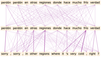
Figure 4: Visualization of Lattice Transformer encoder self-attention and encoder-decoder attention for inference. Top panel: ASR 1-best. Bottom panel: ASR lattice. Target reference: “But in Peru, I’ve heard there are parts where it really gets cold.”

Figure 5: Left panel: ASR 1-best. Right panel: ASR lattice. Target reference: “Yes, yes, I heard it.”

4.1.4 Inference Analysis

On the test datasets of Fisher and Callhome, we make an inference for predicting the translations, and some examples are shown in Table 4. We also visualize the alignment for both encoder self-attention and encoder-decoder attention for the input and predicted translation. Two examples are illustrated in Figure 4 and 5. As expected, the tokens from different paths will not attend to each other, e.g., “pero” and “perdón” in Figure 4 or “hoy” and “y” in Figure 5. In Figure 4, we observe that the 1-best hypothesis can even result in erroneous translation “sorry, sorry”, which is supposed to be “but in peru”. In Figure 5, the translation from 1-best hypothesis obviously misses the important information “i heard it”. We primarily attribute such errors to the insufficient information within 1-best hypothesis, but if the lattice transformer is appropriately trained, the translations from lattice inputs can possibly correct them. Due to limited space, more visualization examples can be found in supplementary material.

Model	Fisher dev2	Fisher test	Callhome evltest
LSTM (1-best input)	37.1	36.6	13.3
Lattice LSTM (lattice input)	36.9	36.1	13.7
+lattice prob scores	38.5	38	14.1
Transformer (1-best input)	38.4	38.5	14.5
Lattice Transformer (lattice input)	38.6	37.9	14.2
+ marginal scores in decoder	39.0	38.7	14.4
+ marginal scores in encoder	38.8	38.2	14.7
+ marginal scores in encoder and decoder	39.5	39.0	14.8
+ marginal scores in encoder and decoder, and forward / backward scores only in encoder self-attention layer 0 and layer 1	39.6	39.1	14.9
+ marginal scores in encoder and decoder, and forward / backward scores in all encoder self-attention layers	39.4	39.2	14.7

Table 5: Ablation Experiment BLEU Results. The rows of the Lattice LSTM and the Lattice Transformer represent the 1-best hypothesis fine-tuning, and the BLEUs are evaluated on 1-best inputs and on lattice inputs for the others. The colored BLEU values come from Table 2 and 3.

4.1.5 Model Ablation Study

We conduct an ablation study to examine the effectiveness of every module in the lattice transformer. We gradually add one module from a standard transformer model to our most complicated lattice transformer. From the results in Table 5, we can see that the application of marginal scores in encoder or decoder has the most influential impact on the lattice fine-tuning. Furthermore, the superimposed application of marginal scores in both encoder and decoder can gain an additional promotion, compared to individual applications. However, the use of forward and backward scores has no significantly extra rewards in this situation. Perhaps due to overfitting, the most complicated lattice transformer on the Callhome of smaller data size cannot achieve better BLEUs than simpler models.

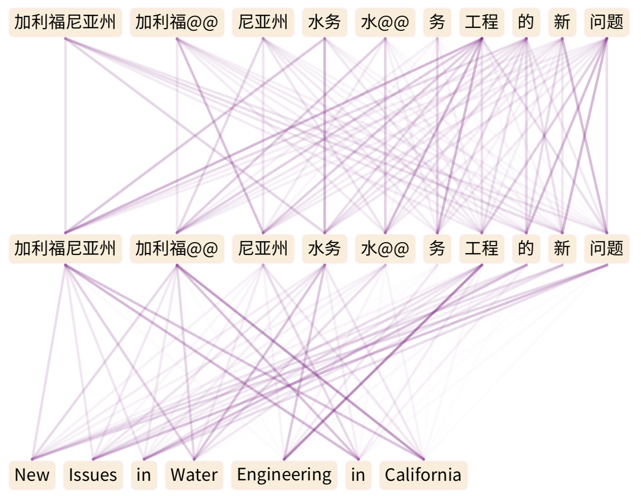
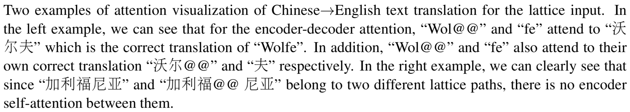
Figure 6: Attention visualization for Chinese English translation task.

4.2 Chinese English Text Translation

Architecture	Inference Inputs	test2017
Transformer Zhang et al. (2018)	BPE 32K	23.01
Transformer-big Hassan et al. (2018)	BPE 32K	24.20
1. Transformer with BPE 32K	BPE 32K	24.26
2. Lattice Transformer from scratch	lattice	24.71
3. Lattice Transformer with fine-tuning	lattice	24.81

Table 6: BLEU on WMT 2017 Chinese English

In this experiment, we demonstrate the performance of our lattice transformer when the probability scores are unavailable. The comparison baseline method is the vanilla transformer Vaswani et al. (2017) in both base and big settings.

4.2.1 Datasets and Settings

The Chinese to English parallel corpus for WMT 2017 news task contains about 20 million sentences after deduplication. For Chinese word segmentation, we use Jieba as the baseline Zhang et al. (2018); Hassan et al. (2018), while the English sentences are tokenized by moses tokenizer. Some data filtering tricks have been applied, such as the ratio within $[1/3,3]$ of lengths between source and target sentence pairs and the count of tokens in both sides ($\leq 200$).

Then for the Chinese source corpus, we learn the BPE tokenization with 16K / 32K / 48K operations, while for the English target corpus, we only learn the BPE tokenization with 32K operations. In this way, each Chinese input can be represented as three different tokenized results, thus being ready to construct a word lattice.

The hyper-parameters of our model are the same as the setting with the speech translation in previous experiments. We follow the optimization convention in Vaswani et al. (2017) to use ADAM optimizer with Noam invert squared decay. All of our lattice transformers are trained on 4 P-100 GPU cards. Similar to our comparison method, detokenized cased-sensitive BLEU is reported in our experiment.

4.2.2 Results

For our lattice transformer, we have three models trained for comparison. First we use the 32K BPE Chinese corpus alone to train our lattice transformer, which is equivalent to the standard transformer with relative positional embeddings. Secondly, we train another lattice transformer with the word lattice corpus from scratch. In addition, we follow the convention of the speech translation task in previous experiments by fine-tuning the first model with word lattice corpus. For each setting, the model evaluated on test 2017 dataset is selected from the best model performed on the dev2017 data. The fine-tuning of Lattice Model 3 starts from the best checkpoint of Lattice Model 1. The BLEU evaluation is shown in Table 6, and two examples of attention visualization are shown in Figure 6. Notice that the first two results of transformer-base and -big are directly copied from the relevant references. From the result, we can see that our Model 1 can be comparable with the vanilla transformer-big model in a base setting, and significantly better than the transformer-base model. We also validate the argument that training from scratch can also achieve a better result than most baselines. Empirically, we find an interesting phenomena that training from scratch converges faster than other settings.

5 Conclusions

In this paper, we propose a novel lattice transformer architecture with a controllable lattice attention mechanism that can consume a word lattice and probability scores from the ASR system. The proposed approach is naturally applied to both the encoder self-attention and encoder-decoder attention. We mainly validate our lattice transformer on speech translation task, and additionally demonstrate its generalization to text translation on the WMT 2017 Chinese-English translation task. In general, the lattice transformer can increase the metric BLEU for translation tasks by a significant margin over many baselines.

References

- Adams et al. (2016) Oliver Adams, Graham Neubig, Trevor Cohn, and Steven Bird. 2016. Learning a translation model from word lattices. In Interspeech.
- Ba et al. (2016) Jimmy Lei Ba, Jamie Ryan Kiros, and Geoffrey E Hinton. 2016. Layer normalization. arXiv preprint arXiv:1607.06450.
- Bojar et al. (2018) Ondřej Bojar, Christian Federmann, Mark Fishel, Yvette Graham, Barry Haddow, Philipp Koehn, and Christof Monz. 2018. Findings of the 2018 conference on machine translation (wmt18). In Proceedings of the Third Conference on Machine Translation: Shared Task Papers, pages 272–303.
- Buckman and Neubig (2018) Jacob Buckman and Graham Neubig. 2018. Neural lattice language models. Transactions of the Association for Computational Linguistics, 6:529–541.
- Devlin et al. (2018) Jacob Devlin, Ming-Wei Chang, Kenton Lee, and Kristina Toutanova. 2018. Bert: Pre-training of deep bidirectional transformers for language understanding. arXiv preprint arXiv:1810.04805.
- Fan et al. (2018) Kai Fan, Bo Li, Fengming Zhou, and Jiayi Wang. 2018. ” bilingual expert” can find translation errors. arXiv preprint arXiv:1807.09433.
- Hassan et al. (2018) Hany Hassan, Anthony Aue, Chang Chen, Vishal Chowdhary, Jonathan Clark, Christian Federmann, Xuedong Huang, Marcin Junczys-Dowmunt, William Lewis, Mu Li, et al. 2018. Achieving human parity on automatic chinese to english news translation. arXiv preprint arXiv:1803.05567.
- He et al. (2016) Kaiming He, Xiangyu Zhang, Shaoqing Ren, and Jian Sun. 2016. Deep residual learning for image recognition. In Proceedings of the IEEE conference on computer vision and pattern recognition, pages 770–778.
- Hochreiter and Schmidhuber (1997) Sepp Hochreiter and Jürgen Schmidhuber. 1997. Long short-term memory. Neural computation, 9(8):1735–1780.
- Jan et al. (2018) Niehues Jan, Roldano Cattoni, Stüker Sebastian, Mauro Cettolo, Marco Turchi, and Marcello Federico. 2018. The iwslt 2018 evaluation campaign. In International Workshop on Spoken Language Translation, pages 2–6.
- Khandelwal et al. (2018) Urvashi Khandelwal, He He, Peng Qi, and Dan Jurafsky. 2018. Sharp nearby, fuzzy far away: How neural language models use context. arXiv preprint arXiv:1805.04623.
- Kudo (2018) Taku Kudo. 2018. Subword regularization: Improving neural network translation models with multiple subword candidates. In Proceedings of the 56th Annual Meeting of the Association for Computational Linguistics (Volume 1: Long Papers), volume 1, pages 66–75.
- Lample et al. (2018) Guillaume Lample, Myle Ott, Alexis Conneau, Ludovic Denoyer, et al. 2018. Phrase-based & neural unsupervised machine translation. In Proceedings of the 2018 Conference on Empirical Methods in Natural Language Processing, pages 5039–5049.
- Osamura et al. (2018) Kaho Osamura, Takatomo Kano, Sakriani Sakti, Katsuhito Sudoh, and Satoshi Nakamura. 2018. Using spoken word posterior features in neural machine translation. architecture, 21:22.
- Post et al. (2013) Matt Post, Gaurav Kumar, Adam Lopez, Damianos Karakos, Chris Callison-Burch, and Sanjeev Khudanpur. 2013. Improved speech-to-text translation with the fisher and callhome spanish–english speech translation corpus. In International Workshop on Spoken Language Translation.
- Rabiner (1989) Lawrence R Rabiner. 1989. A tutorial on hidden markov models and selected applications in speech recognition. Proceedings of the IEEE, 77(2):257–286.
- Sennrich et al. (2016) Rico Sennrich, Barry Haddow, and Alexandra Birch. 2016. Neural machine translation of rare words with subword units. In Proceedings of the 54th Annual Meeting of the Association for Computational Linguistics (Volume 1: Long Papers), volume 1, pages 1715–1725.
- Shaw et al. (2018) Peter Shaw, Jakob Uszkoreit, and Ashish Vaswani. 2018. Self-attention with relative position representations. In Proceedings of the 2018 Conference of the North American Chapter of the Association for Computational Linguistics: Human Language Technologies, Volume 2 (Short Papers), volume 2, pages 464–468.
- Sperber et al. (2017) Matthias Sperber, Graham Neubig, Jan Niehues, and Alex Waibel. 2017. Neural lattice-to-sequence models for uncertain inputs. In Proceedings of the 2017 Conference on Empirical Methods in Natural Language Processing, pages 1380–1389.
- Su et al. (2017) Jinsong Su, Zhixing Tan, Deyi Xiong, Rongrong Ji, Xiaodong Shi, and Yang Liu. 2017. Lattice-based recurrent neural network encoders for neural machine translation. In Thirty-First AAAI Conference on Artificial Intelligence.
- Su et al. (2018) Yuanhang Su, Kai Fan, Nguyen Bach, C-C Jay Kuo, and Fei Huang. 2018. Unsupervised multi-modal neural machine translation. arXiv preprint arXiv:1811.11365.
- Sutskever et al. (2014) Ilya Sutskever, Oriol Vinyals, and Quoc V Le. 2014. Sequence to sequence learning with neural networks. In Advances in neural information processing systems, pages 3104–3112.
- Tai et al. (2015) Kai Sheng Tai, Richard Socher, and Christopher D Manning. 2015. Improved semantic representations from tree-structured long short-term memory networks. In Proceedings of the 53rd Annual Meeting of the Association for Computational Linguistics and the 7th International Joint Conference on Natural Language Processing (Volume 1: Long Papers), volume 1, pages 1556–1566.
- Vaswani et al. (2017) Ashish Vaswani, Noam Shazeer, Niki Parmar, Jakob Uszkoreit, Llion Jones, Aidan N Gomez, Łukasz Kaiser, and Illia Polosukhin. 2017. Attention is all you need. In Advances in Neural Information Processing Systems, pages 5998–6008.
- Yu et al. (2018) Adams Wei Yu, David Dohan, Minh-Thang Luong, Rui Zhao, Kai Chen, Mohammad Norouzi, and Quoc V Le. 2018. Qanet: Combining local convolution with global self-attention for reading comprehension. arXiv preprint arXiv:1804.09541.
- Zhang and Yang (2018) Yue Zhang and Jie Yang. 2018. Chinese ner using lattice lstm. In Proceedings of the 56th Annual Meeting of the Association for Computational Linguistics (Volume 1: Long Papers), volume 1, pages 1554–1564.
- Zhang et al. (2018) Zhirui Zhang, Shuangzhi Wu, Shujie Liu, Mu Li, Ming Zhou, and Enhong Chen. 2018. Regularizing neural machine translation by target-bidirectional agreement. arXiv preprint arXiv:1808.04064.