Relating microswimmer synthesis to hydrodynamic actuation and rheotactic tunability

Abstract

We explore the behavior of micron-scale autophoretic Janus (Au/Pt) rods, having various Au/Pt length ratios, swimming near a wall in an imposed background flow. We find that their ability to robustly orient and move upstream, i.e. to rheotax, depends strongly on the Au/Pt ratio, which is easily tunable in synthesis. Numerical simulations of swimming rods actuated by a surface slip show a similar rheotactic tunability when varying the location of the surface slip versus surface drag. Slip location determines whether swimmers are Pushers (rear-actuated), Pullers (front-actuated), or in between. Our simulations and modeling show that Pullers rheotax most robustly due to their larger tilt angle to the wall, which makes them responsive to flow gradients. Thus, rheotactic response infers the nature of difficult to measure flow-fields of an active particle, establishes its dependence on swimmer type, and shows how Janus rods can be tuned for flow responsiveness. We demonstrate the effectiveness of a simple geometric sieve for rheotactic ability.

Swimming microorganisms must contend with boundaries and obstacles in their natural environments Saintillan and Shelley (2013); Goldstein (2016); Blechinger et al. (2016). Microbial habitats have ample surfaces, and swimmer concentrations near them promote attachment and biofilms Rusconi and Stocker (2015); Conrad and Poling-Skutvik (2018). Motile bacteria and spermatozoa accumulate near boundaries, move along them Berke et al. (2008); Elizabeth Hulme et al. (2008), and self-organize under confinement Denissenko et al. (2012); Vladescu et al. (2014); Lushi et al. (2014); Wioland et al. (2016). Microswimmers also exhibit rheotaxis, i.e. the ability to actively reorient and swim against an imposed flow Marcos et al. (2012). Surfaces are key for rheotactic response: fluid shear near boundaries results in hydrodynamic interactions which favor swimmer alignment against the oncoming flow and prevent swimmer displacements across streamlines Hill et al. (2007); Kaya and Koser (2012); Costanzo et al. (2012); Kantsler et al. (2014); Figueroa-Morales et al. (2015). Swimmers with different propulsion mechanisms – front-actuated like puller micro-algae, or rear-actuated like pusher bacteria – exhibit associated dipolar flow fields Purcell (1977); Drescher et al. (2011, 2010) which result in dissimilar collective motions Dombrowski et al. (2004); Saintillan and Shelley (2007, 2012) and behavior near boundaries or in flows Spagnolie and Lauga (2012); Zöttl and Stark (2012); Contino et al. (2015); Lushi et al. (2017); Bianchi et al. (2017); Mathijssen et al. (2018).

Recent advances in the manufacture and design of artificial swimmers have triggered an acute interest in developing synthetic mimetic systems Paxton et al. (2006); Howse et al. (2007); Moran and Posner (2011); Duan et al. (2015); Blechinger et al. (2016); Moran and Posner (2017). Like their biological counterparts, artificial swimmers can accumulate near boundaries Takagi et al. (2014); Brown et al. (2016), navigate along them Das et al. (2015); Liu et al. (2016), be guided by geometric or chemical patterns Simmchen et al. (2016); Uspal et al. (2016); Davies-Wykes et al. (2017); Tong and Shelley (2018) or external forces Tierno et al. (2008); Garcia-Torres et al. (2018), and can display rheotaxis near planar surfaces Uspal et al. (2015); Palacci et al. (2015); Ren et al. (2017). While models have been developed to study their locomotion and behavior Spagnolie and Lauga (2012); Takagi et al. (2014); Spagnolie et al. (2015); Potomkin et al. (2017), the relevance of the swimmers’ actuation mechanism and the resulting hydrodynamic contributions to their rheotactic motion remains an open question. In large part this is due to the difficulty in directly assessing swimmers’ flow-fields, particularly near walls, and relating experimental observations to our theoretical understanding of swimmer geometry, hydrodynamics and type (i.e., pusher or puller).

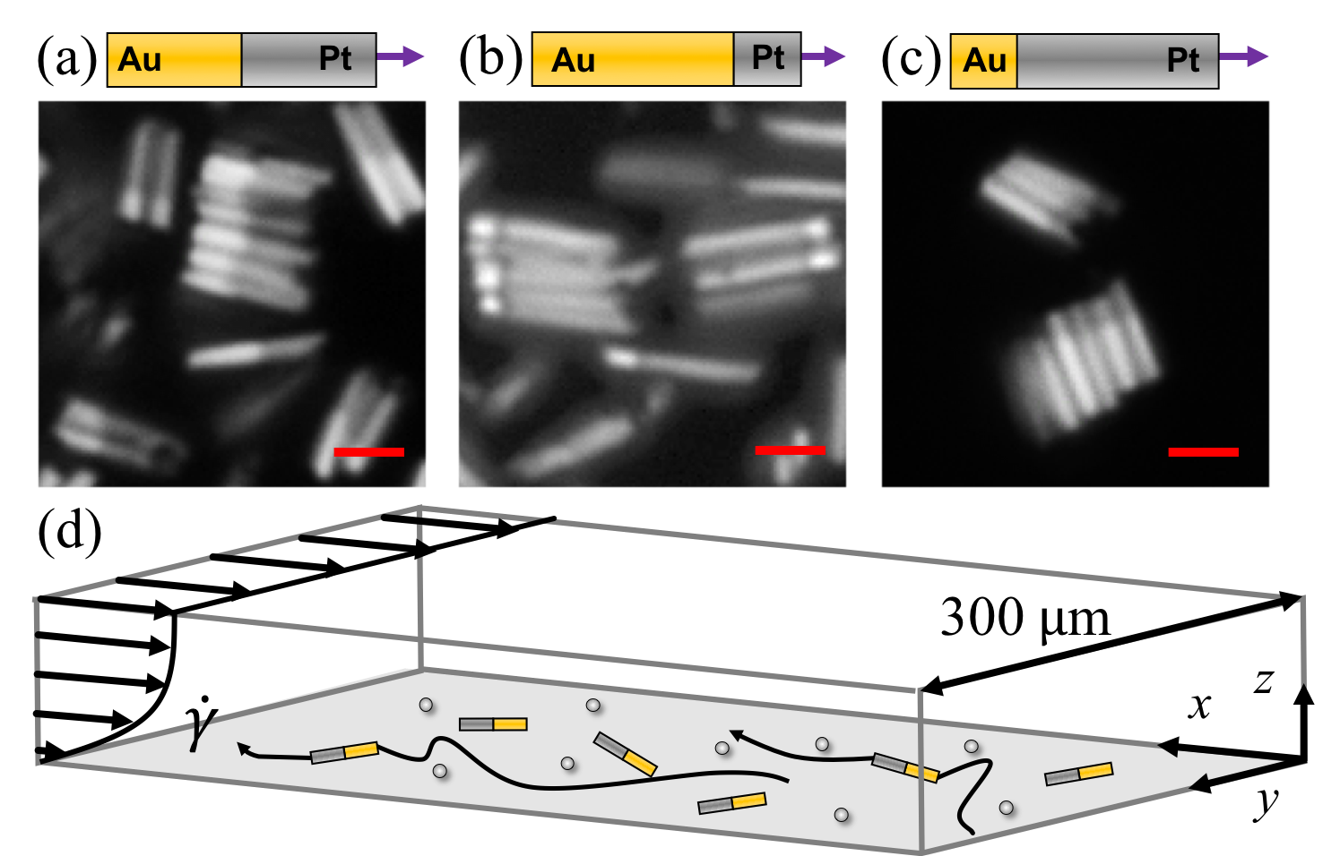
Figure 1: The different bimetallic swimmers. The ratio of the metallic segments varies from (a) 1:1 for symmetric, to (b) 3:1 for long-gold and to (c) 1:3 for long-platinum. Scale bar $1\mu m$. (d) Each swimmer type is tested in a rectangular microfluidic channel where it is gravitationally confined near the bottom. Under shear flow the metallic particles swim upstream.

In this Letter, we address this question with experiments using chemically powered gold-platinum (Au/Pt) microswimmers combined and compared with numerical simulations. In experiments we vary the position of the Au/Pt join along the swimmer length, postulating that this varies the location of the flow actuation region, and that observed differences in rheotaxis can be related to having different pusher- or puller-like swimmers. In simulation, we study the rheotactic responses of rod-like microswimmers that move through an active surface slip. Different placements of the slip region allow us to create pullers, symmetric, and pusher microswimmers. We find measurably different rheotactic responses in simulation which show quantitative agreement with our experiments with Au/Pt active particles conducted in microfluidic channels. Lastly, we show that mixed swimmer populations can be sorted through a microfluidic sieve that exploits the swimmers’ different rheotactic behaviors.

Experimental setup and measurements. Our Janus microswimmers are elongated Au/Pt rods, $\sim 2\mu m$ in length and $\sim 0.3\mu m$ in diameter, which propel themselves through self-electrophoresis in aqueous H₂O₂ solutions Moran and Posner (2011, 2017). The swimmers are synthesized by electrodeposition Paxton et al. (2006); Banholzer et al. (2009) to a prescribed ratio of the two metallic segments: symmetric with Au:Pt (1:1), asymmetric long-gold with Au:Pt (3:1) and asymmetric long-platinum with Au:Pt (1:3); see Fig. 1a-c, details in Sup .

The swimmers’ rheotactic abilities are tested in a rectangular PDMS microfluidic channel of width $W=300\mu m$ built following classical soft-lithography techniques Qin et al. (2010). We control the background unidirectional flow down the channel (the $x$-direction) using an off-stage hydrostatic column. Suspended glass beads of radius $r_{b}\sim 2.5\mu m$ serve as markers to measure the flow profile close to the bottom of the channel where the rods move. We record the trajectories of swimmers and beads over 1 minute and extract the instantaneous velocities of swimmers $V_{x}$ and of beads $U_{b}$, along the $x$-axis. See Fig. 1d and videos in Sup .

Thermal fluctuations are important at this scale and the swimmers mean square displacement for $U_{0}=0$ at a fixed H₂O₂ concentration are used to estimate their translational and rotational diffusivities, $D_{t}$ and $D_{r}$, and deterministic base-line swimming speeds $V_{0}$ Howse et al. (2007); Sup . At fixed H₂O₂ concentration, swimming speeds are smaller for asymmetric rods than for symmetric ones, therefore H₂O₂ concentration is adjusted to maintain a comparable velocity $V_{0}$ between experiments.

The background flow profile close to the wall $U_{0}(z)$ is measured by the drift velocity $U_{b}$ of the suspended glass beads. As the beads move close to the wall, we find it important to account for the lubrication forces that act upon them Goldman et al. (1967). The flow velocity is estimated to be $U_{0}(r_{b}+h_{th})\sim 2.5U_{b}$ for a thermal height $h_{th}\sim 30nm$Sup .

Model and Simulations. Resolving the chemical and electro-hydrodynamics near a wall is challenging. The electro-osmotic flow near an self-diffusiophoretic swimmer is the result of charge gradients localized on a small surface region near the junction of the two metallic segments Paxton et al. (2006). We make the simplifying assumption that this results in a surface slip velocity yielding the rod propulsion with the Pt segment leading. As we do not know the extent of the slip region, we simply assume that it covers half the rod length. The propulsion speed depends on the slip coverage.

We model the swimmer as a rigid, axisymmetric rod immersed in a Stokes flow and sedimented near an infinite substrate. The rod is discretized using $N_{b}$ “blobs” at positions $(\bm{r}_{i}-\bm{q})$ with respect to the rod center $\bm{q}$ Delong et al. (2015); Balboa Usabiaga et al. (2016). Linear and angular velocities $\bm{u}$ and $\bm{\omega}$ satisfy the linear system Eqs. (1,2) where $\bm{\lambda}_{i}$ are unknown constraint forces enforcing rigid body motion and $\bm{M}$ is the Rotne-Prager mobility tensor Rotne and Prager (1969) corrected to include the hydrodynamic effect of the substrate Blake (1971); Swan and Brady (2007).

Eq. (1) represents the balance of the geometric constraint forces with the external force $\bm{F}$ and torque $\bm{\tau}$ generated by steric interactions with the substrate and gravity. Eq. (2) gives the balance of fluid, propulsive, and thermal forces, with $\widetilde{\bm{u}}_{i}$ the active slip velocity, $\bm{u}_{0}(\bm{r}_{i})$ the background flow velocity, and $\sqrt{2k_{B}T/\Delta t}(\bm{M}^{1/2}\bm{W})_{i}$ the Brownian noise, with $k_{B}$ the Boltzmann constant, $T$ the temperature, $\Delta t$ the time step, $\bm{W}$ a vector of white noises, and $\bm{M}^{1/2}$ representing the square root of the mobility tensor Ando et al. (2012). Half the blobs along the rod are “passive” with $\widetilde{\bm{u}}_{i}=0$, while the other half have an active slip of constant magnitude $|\widetilde{\bm{u}}_{i}|=u_{s}$ parallel to the rod’s main axis. We can set the active slip at the rear, middle, or front; See Fig. 2a-c. After solving Eqs. (1,2), we update the configuration with a stochastic integrator Sprinkle et al. (2017). Here, the background flow is linear shear: $\bm{u}_{0}({\bf x})=\dot{\gamma}z\hat{\bf{x}}$.

$$\sum_{i\in(1,N_{b})}\bm{\lambda}_{i}=\bm{F},\quad\quad\sum_{i\in(1,N_{b})}(\bm{r}_{i}-\bm{q})\times\bm{\lambda}_{i}=\bm{\tau},$$ (1)

$$\sum_{j\in(1,N_{b})}\bm{M}_{ij}\bm{\lambda}_{j}=\bm{u}+\bm{\omega}\times(\bm{r}_{i}-\bm{q})-\bm{u}_{0}(\bm{r}_{i})+\widetilde{\bm{u}}_{i}+$$ (2)

$$\sqrt{2k_{B}T/\Delta t}\left(\bm{M}^{1/2}\bm{W}\right)_{i}\;\mbox{for }i\in(1,N_{b}).$$

Fig. 2b & c show that asymmetrically placed slip results in a contractile (or puller) dipolar flow for front-slip particles, and an extensile (or pusher) dipolar flow for rear-slip particles. The former corresponds to physical long-gold particles, and the latter to short-gold. Placing the slip region in the middle (symmetric swimmers) – see Fig. 2a – yields a higher-order Stokes quadrupole flow as its leading order contribution. This corresponds to a symmetric Au/Pt particle.

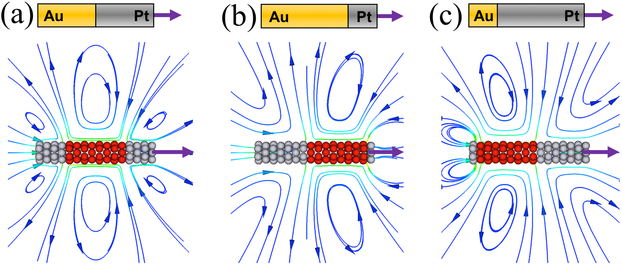
Figure 2: Computed velocity fields around simulated self-propelled rods with a surface slip region (shown in red) (a) at the center, (b) at the front, and (c) at the rear, corresponding to, symmetric, puller and pusher swimmers, respectively.

Simulation results To build intuition, we first explore the simulations’ predictions, which motivate a yet simpler dynamical model of rheotactic response.

Fig. 3a illustrates the basic rheotactic response evinced by our microswimmer model for all swimmer types (pusher, symmetric, puller). Here, Brownian fluctuations are neglected, and all swimmers are initially set to swim downstream in a linear shear flow. In reaction to the background shear each swimmer turns to swim upstream, with the pusher being the least responsive. For symmetric swimmers, Fig. 3b shows the competition between rheotaxis induced by flow with thermal fluctuations whose effect is to de-correlate the swimming direction. In the absence of background flow ($\dot{\gamma}=0$), swimmers diffuse isotropically over long times. This yields a symmetric bimodal distribution $P(V_{x})$ for the $x$-velocity $V_{x}$. As the shear-rate becomes increasingly positive, the distribution becomes asymmetric and increasingly biased towards upstream swimming (negative $V_{x}$). The distribution curves also shift right, yielding smaller peak upstream velocities and larger peak downstream velocities.

Simulations show that active rods swim with a downward tilt towards the substrate, i.e. with their Pt head segment closer to the wall Takagi et al. (2014); Ren et al. (2017). The tilt angle $\alpha$ depends weakly on the shear rate but is different for puller, pusher and symmetric swimmers, see Fig. 3c. It is this tilt that allows the microswimmer to respond to the shear flow near the wall, and is the origin of rheotaxis.

The fact of a nonzero tilt angle has been explored most thoroughly by Spagnolie & Lauga Spagnolie and Lauga (2012) who, in seeking to understand capture of active particles by spherical obstacles Takagi et al. (2014), numerically studied idealized ellipsoidal “squirmers” moving near a spherical surface. For our numerical model we associate the tilt with the appearance of high (and low) pressure regions between the swimming rod and the substrate that tilt the swimmer. These regions appear where surface velocities, both from slip and no-slip regions, are converging (and diverging). Moving the slip/no-slip boundary moves the high pressure region, and thus changes the tilt angle (see Sup ).

A weather-vane model From these observations we build an intuitive model displaying a behavior akin to that of a weathervane. Due to its downward tilt, the shear flow imposes a larger drag on the tail of a swimming rod. The drag differential promotes upstream orientation by producing a torque that depends on the tilt angle $\alpha$. The rod’s planar position $\bm{x}=(x,y)$ and orientation angle $\theta$ evolve as:

$${\bm{\dot{x}}}=V_{0}{\bm{n}(\theta)}+\dot{\gamma}h{\bm{e}_{x}}+\sqrt{2D_{t}}{\bm{W}_{x}},$$ (3)

$$\dot{\theta}=\dot{\gamma}\sin\alpha\sin\theta+\sqrt{2D_{r}}W_{\theta}.$$ (4)

Eq. (3) describes a swimming rod that moves with intrinsic speed $V_{0}$ at an angle $\theta$ [$\bm{n}=(\cos(\theta),\sin(\theta))$], while is advected by a shear flow with speed $\dot{\gamma}h$ at a characteristic height $h$ along the $x$-axis. Eq. 4 imposes that the rod angle $\theta$ orients against the shear flow. The particle’s translational and angular diffusion are $D_{t}$ and $D_{r}$. $\bm{W}_{x}$ and $W_{\theta}$ are uncorrelated white noise processes.

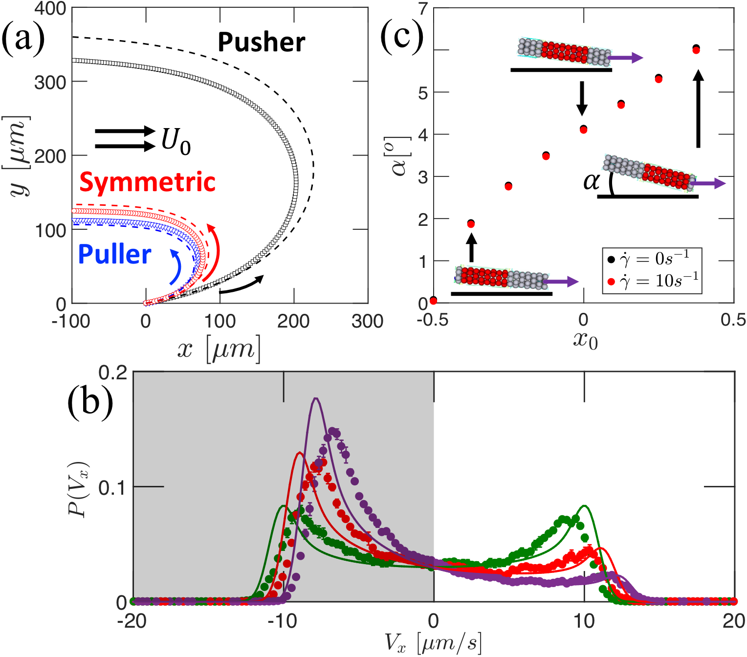
Figure 3: (a) Trajectories of deterministic swimmers with initial orientation $\theta_{0}=\pi/16$, seen from above for simulations (solid lines) and theory (dashed lines). (b) Particle velocity distribution in the flow direction ($V_{x}$) for hydrodynamic simulations with brownian noise in a shear flow with $\dot{\gamma}$=0$s^{-1}$ ($\color[rgb]{0,1,0}\bullet$), 4$s^{-1}$ ($\color[rgb]{1,0,0}\bullet$) and 8$s^{-1}$ ($\color[rgb]{0.5,0.0,0.9}\bullet$), and weathervane model (lines). (c) From simulations, equilibrium tilt angle relative to the substrate $\alpha$ as a function of the center of the slip layer $x_{0}$ (with $x_{0}=+0.5,0,-0.5$ representing front/middle/aft slip).

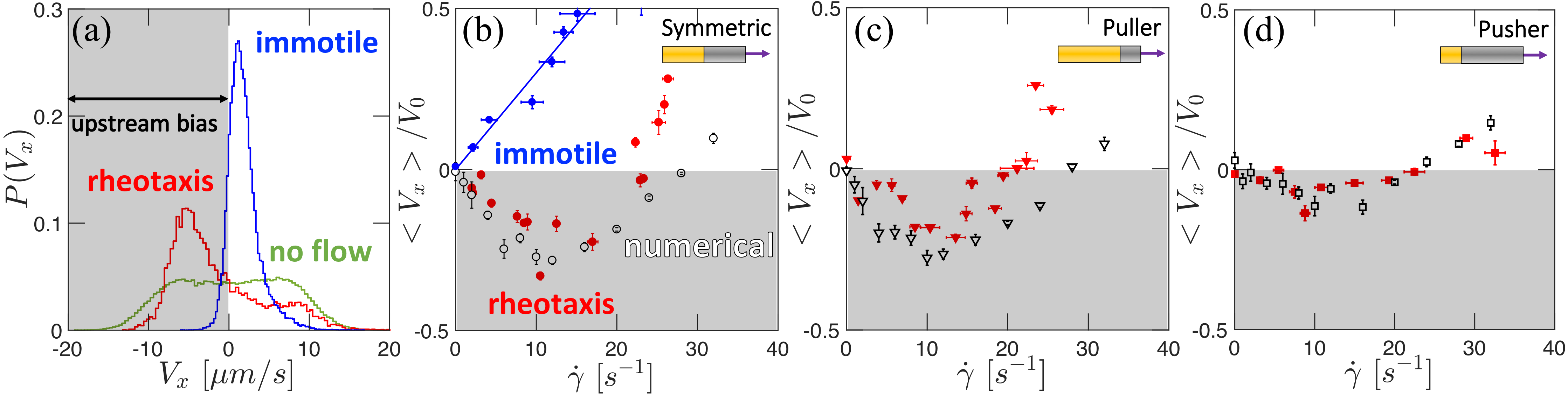
Figure 4: (a) From experiments: velocity distribution $P(V_{x})$ of symmetric swimmers in the absence of background flow ($\color[rgb]{0,1,0}-$), with background flow $\dot{\gamma}=8.7s^{-1}$ ($\color[rgb]{1,0,0}-$) and for immotile particles in flow $\dot{\gamma}=9.5s^{-1}$ ($\color[rgb]{0,0,1}-$). Mean velocity vs. shear rates for (b) symmetric, (c) long-gold puller, and (d) long platinum pusher swimmers respectively in experiments ($\color[rgb]{1,0,0}+$) and simulations ($\color[rgb]{0,0,0}\circ$) and compared to experiment with immotile particles ($\color[rgb]{0,0,1}+$). Region of upstream swimming bias is shaded in gray.

This model is sufficient to reproduce the deterministic trajectories of symmetric, puller and pusher swimmers, Fig. 3a. The tilt angle $\alpha$ controls how fast a rod reorients against the flow and it explains why pushers are less responsive to shear flows. The model also predicts a critical swimming speed to observe positive rheotaxis (upstream swimming). As $\dot{\gamma}\rightarrow 0$, the average velocity along the flow is $\langle V_{x}\rangle=\dot{\gamma}\left(h-V_{0}\sin\alpha/2D_{r}\right)$ which sets the critical speed $V_{0c}=2D_{r}h/\sin\alpha$ where the role of the tilt angle is evident.

From Eqs. (3)-(4) we derive the distribution $P(V_{x})$ of the swimmer velocities down the channel Sup , see Fig. 3b. Although the weathervane model neglects hydrodynamics interactions with the substrate, it agrees with the full numerical simulations for the range of shear rates and also underlines the influence of parameters influencing rheotaxis. Note that the absence of lubrication forces results in an overestimated swimmer velocity in the $x$-direction, a discrepancy reflected in the distribution peaks shifted to larger absolute values of $V_{x}$.

Experimental validation of the theory. In experiments the velocity distribution $P(V_{x})$ follows the same phenomenology described for the numerical simulations and the reduced model; see Fig.4a. Under weak shear flow we observe that passive particles (i.e. no H₂O₂) are washed downstream whereas all three types of active rods orient themselves against the flow and swim upstream.

As suggested by Fig. 3a, both experiments and simulations reveal that pushers are the least robust rheotactors. Upstream swimming bias is measured by $\langle V_{x}\rangle$ as a function of the shear rate, shown in Fig. 4b-d. Upstream rheotaxis is found for moderate shear rates, $\dot{\gamma}<20-30\mbox{s}^{-1}$, with the characteristic non-monotonic trends previously described Palacci et al. (2015); Ren et al. (2017). The swimmers’ ability to move against the flow reaches a maximum at $\dot{\gamma}\sim 10$\mathrm{s}^{-1}$$. When the viscous drag overcomes the propulsive forces, i.e. $\dot{\gamma}>20$\mathrm{s}^{-1}$$, the rods enter a drifting regime characterized by a rectilinear downstream motion ($\langle V_{x}\rangle>0$). For large shear rates the reduced model predicts a linear average velocity $\langle V_{x}\rangle\sim-V_{0}+h\dot{\gamma}$. This trend is consistent with numerical and experimental results of Fig. 4b-d beyond the minimum of $\langle V_{x}\rangle$, though with slightly different slopes. Even in the drifting regime the average speed $\langle V_{x}\rangle$, of active particles is smaller than immotiles ones because they are directed and swimming upstream.

Both the symmetric and asymmetric swimmers’ rheotactic behavior agrees with the numerical predictions. This result corroborates the partial slip model used in the numerical model to describe asymmetric Au/Pt distributions. Qualitatively, simulations indicate that the maximum velocity upstream should be larger for puller and symmetric swimmers than for pushers. Experiments found roughly a factor of two difference between the maximum upstream velocities between pushers and pullers at comparable shear values, implying that the reorienting torque is strongest for pullers. This observation further agrees with the deterministic trajectories presented in Fig. 3a. There, the parameter that differentiates those swimmers’ dynamics is their tilt angle $\alpha$, identifying it as a crucial parameter to engineer efficient rheotactors.

A rheotactor sieve. Fig. 5a presents the concept of a “microfluidic sieve” consisting of a diverging channel. A constant fluid influx yields a decreasing shear gradient downstream. We show that in limited windows of flow-rates, the rheotactors travel upstream in the nozzle until facing a “shear wall” that prevents them from traveling further, thus concentrating them in those locations.

Fig. 5b compares the symmetric swimmers’ local density integrated over a period of three minutes for two different shear regimes. The local swimmer density, $\rho_{l}$ along the $x$-direction is normalized by the average density within the channel, $\rho_{tot}$, to compare experiments with different total numbers of microswimmers. For small flow-rates (blue), rheotactors swim upstream at any point of the nozzle. The population density is evenly distributed within the whole channel as the velocity of the swimmers changes little in this range of induced shear. In a critical regime (red), the swimmers drift downstream from the narrow part of the channel but swim upstream in the wider sections. The change of sign in the local average swimmer velocity corresponds roughly with a peak of swimmer density, showing the accumulation of the swimmers in this region Fig. 5b (arrow). This geometry allows the sorting of motile swimmers based on their speed or tilt angle. From the examples presented above, this method could conveniently separate mixed populations of asymmetric swimmers in the same channel.

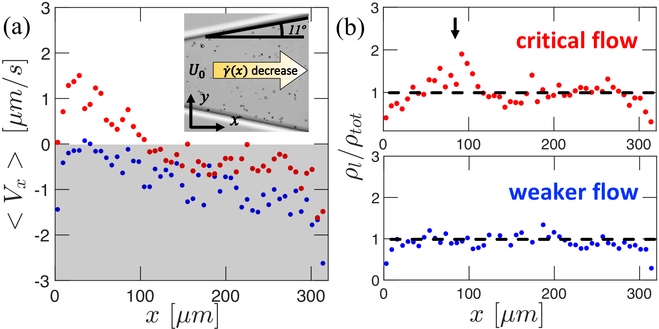
Figure 5: A rheotactor sieve: (a) The local mean swimmer velocity for critical (${\color[rgb]{1,0,0}\bullet}$) and low (${\color[rgb]{0,0,1}\bullet}$) flow rates in a microfluidic sieve geometry (inset). At the critical flow rate, particles swim upstream in the wide part of the channel and downstream in the narrow part. (b) The time-integrated swimmer density profile normalised by the average swimmer density $\rho_{l}/\rho_{tot}$ reveals a concentration of swimmers where the mean swimmer velocity changes sign (indicated by an arrow).

Discussion. Through experiment, simulation, and modeling, we demonstrate how to modify rheotactic response by changing swimmer type, which for Au/Pt Janus rods amounts to changing the location of the Au/Pt join. Rheotactic tunability is determined primarily by the tilt angle of the swimmer to the wall, which is controlled by the distribution of the surface slip. The quantitative agreement between experiment and simulation demonstrates that we can infer “by proxy” the pusher and puller nature of artificial microswimmers for which direct flow visualisation is often difficult to obtain. Our study extends and elaborates upon the recent results of Ren et al. (Ren et al., 2017) on rheotaxis of symmetric Janus swimmers.

It is chemical reactions that determine the active surface regions. However, our modeling work here, and that of others Spagnolie and Lauga (2012), show that swimmer-substrate hydrodynamic interactions are sufficient to produce a tilt angle of the rods and thus yield rheotaxis. Our conclusions should apply to other swimmer types besides phoretic particles. A careful treatment of the electro-chemical reactions could refine the model of the active slip region used in this work, though solving the electro-chemical reactions in the presence of thermal fluctuations is far from trivial Moran and Posner (2011).

The placement of the slip region opens other routes to design artificial swimmers that have specific interactions with obstacles. For example, particles that swim with their heads up at a wall will tend to move away from it Spagnolie and Lauga (2012). To explore this idea we numerically designed swimmers that will tilt up Sup by placing an active slip region that covers the nose back to a point forward of the midpoint. This yields a single high pressure node in the front half that tilts up the rod. Placing the slip region on the back half creates a low pressure node on the back half, yielding the same effect. How to experimentally produce Au/Pt swimmers with such slip distributions is an interesting question that we are investigating now.

Acknowledgements. This work was supported by NSF-MRSEC program DMR-1420073, and NSF Grants DMS-1463962 and DMS-1620331.

References

- Saintillan and Shelley (2013) D. Saintillan and M. E. Shelley, Comp. Rend. Phys. (2013).
- Goldstein (2016) R. E. Goldstein, Journal of Fluid Mechanics 807, 1 (2016).
- Blechinger et al. (2016) C. Blechinger, R. Di Leonardo, H. Löwen, C. Reichhardt, G. Volpe, and G. Volpe, Rev. Mod. Phys. 88, 045006 (2016).
- Rusconi and Stocker (2015) R. Rusconi and R. Stocker, Curr. Op. Micro. 25, 1 (2015).
- Conrad and Poling-Skutvik (2018) J. Conrad and R. Poling-Skutvik, Annu. Rev. Chem. Biomol. Eng. 9, 175 (2018).
- Berke et al. (2008) A. Berke, L. Turner, H. Berg, and E. Lauga, Phys. Rev. Lett. 101, 038102 (2008).
- Elizabeth Hulme et al. (2008) S. Elizabeth Hulme, W. R. DiLuzio, S. S. Shevkoplyas, L. Turner, M. Mayer, H. C. Berg, and G. M. Whitesides, Lab Chip 8, 1888 (2008).
- Denissenko et al. (2012) P. Denissenko, V. Kantsler, D. J. Smith, and J. Kirkman-Brown, Proc. Natl. Acad. Sci. 109, 8007 (2012).
- Vladescu et al. (2014) I. Vladescu, E. Marsden, J. Schwarz-Linek, V. Martinez, J. Arlt, A. N. Morozov, D. Marenduzzo, M. Cates, and W. C. K. Poon, Phys. Rev. Lett 113, 268101 (2014).
- Lushi et al. (2014) E. Lushi, H. Wioland, and R. Goldstein, Proc. Nat. Acad. Sci. 111, 9733 (2014).
- Wioland et al. (2016) H. Wioland, E. Lushi, and R. Goldstein, New J. Phys. 18, 075002 (2016).
- Marcos et al. (2012) M. Marcos, H. C. Fu, T. R. Powers, and R. Stocker, Proc. Nat. Acad. Sci. (2012), ISSN 0027-8424.
- Hill et al. (2007) J. Hill, O. Kalkanci, J. L. McMurry, and H. Koser, Phys. Rev. Lett. 98, 068101 (2007).
- Kaya and Koser (2012) T. Kaya and H. Koser, Biophys. J. 102, 1514 (2012).
- Costanzo et al. (2012) A. Costanzo, R. Di Leonardo, G. Ruocco, and L. Angelani, J. Phys.: Cond. Matt. 24, 065101 (2012).
- Kantsler et al. (2014) V. Kantsler, J. Dunkel, M. Blayney, and R. E. Goldstein, eLife 111 (2014).
- Figueroa-Morales et al. (2015) N. Figueroa-Morales, G. Leonardo Mino, A. Rivera, R. Caballero, E. Clement, E. Altshuler, and A. Lindner, Soft Matt. 11, 6284 (2015).
- Purcell (1977) E. M. Purcell, Am. J. Phys. 45, 3 (1977).
- Drescher et al. (2011) K. Drescher, J. Dunkel, L. H. Cisneros, S. Ganguly, and R. E. Goldstein, Proc. Nat. Acad. Sci. 108, 10940 (2011).
- Drescher et al. (2010) K. Drescher, R. E. Goldstein, N. Michel, M. Polin, and I. Tuval, Phys. Rev. Lett. 105, 168101 (2010).
- Dombrowski et al. (2004) C. Dombrowski, L. Cisneros, S. Chatkaew, R. Goldstein, and K. J.O., Phys. Rev. Lett. 93, 098103 (2004).
- Saintillan and Shelley (2007) D. Saintillan and M. E. Shelley, Phys. Rev. Lett. 99, 058102 (2007).
- Saintillan and Shelley (2012) D. Saintillan and M. J. Shelley, J. Royal Soc. Int. 9, 571 (2012).
- Spagnolie and Lauga (2012) S. E. Spagnolie and E. Lauga, J. Fluid Mech. 700, 105 (2012).
- Zöttl and Stark (2012) A. Zöttl and H. Stark, Phys. Rev. Lett. 108, 218104 (2012).
- Contino et al. (2015) M. Contino, E. Lushi, I. Tuval, V. Kantsler, and M. Polin, Phys. Rev. Lett. 115, 258102 (2015).
- Lushi et al. (2017) E. Lushi, V. Kantsler, and R. E. Goldstein, Phys. Rev. E 96, 023102 (2017).
- Bianchi et al. (2017) S. Bianchi, F. Saglimbeni, and R. Di Leonardo, Phys. Rev. X 7, 011010 (2017).
- Mathijssen et al. (2018) A. Mathijssen, N. Figueroa-Morales, G. Junot, E. Clement, A. Lindner, and A. Zoettl, arXiv p. :1803.01743 (2018).
- Paxton et al. (2006) W. F. Paxton, P. T. Baker, T. R. Kline, Y. Wang, T. E. Mallouk, and A. Sen, J. Am. Chem. Soc. 128, 14881 (2006).
- Howse et al. (2007) J. R. Howse, R. A. L. Jones, A. J. Ryan, T. Gough, R. Vafabakhsh, and R. Golestanian, Phys. Rev. Lett. 99, 048102 (2007).
- Moran and Posner (2011) J. L. Moran and J. D. Posner, J. Fluid Mech. 680, 31 (2011).
- Duan et al. (2015) W. Duan, W. Wang, S. Das, V. Yadav, T. E. Mallouk, and A. Sen, Ann. Rev. of Ana. Chem. 8, 311 (2015).
- Moran and Posner (2017) J. L. Moran and J. D. Posner, Ann. Rev. Fluid Mech. 49, 511 (2017).
- Takagi et al. (2014) D. Takagi, J. Palacci, A. B. Braunschweig, M. J. Shelley, and J. Zhang, Soft Matt. 10, 1784 (2014).
- Brown et al. (2016) A. T. Brown, I. D. Vladescu, A. Dawson, T. Vissers, J. Schwarz-Linek, J. S. Lintuvuori, and W. C. K. Poon, Soft Matt. 12, 131 (2016).
- Das et al. (2015) S. Das, A. Garg, A. I. Campbell, J. Howse, A. Sen, D. Velegol, R. Golestanian, and S. J. Ebbens, Nat. Comm. 6, 8999 (2015).
- Liu et al. (2016) C. Liu, C. Zhou, W. Wang, and H. P. Zhang, Phys. Rev. Lett. 117, 198001 (2016).
- Simmchen et al. (2016) J. Simmchen, J. Katuri, W. E. Uspal, M. N. Popescu, M. Tasinkevych, and S. Sánchez, Nat. Comm. 7, 10598 (2016).
- Uspal et al. (2016) W. E. Uspal, M. N. Popescu, S. Dietrich, and M. Tasinkevych, Phys. Rev. Lett. 117, 048002 (2016).
- Davies-Wykes et al. (2017) M. S. Davies-Wykes, X. Zhong, J. Tong, T. Adachi, Y. Liu, L. Ristroph, M. D. Ward, M. J. Shelley, and J. Zhang, Soft Matt. 13, 4681 (2017).
- Tong and Shelley (2018) J. Tong and M. Shelley, SIAM Journal on Applied Mathematics 78, 2370 (2018).
- Tierno et al. (2008) P. Tierno, R. Golestanian, I. Pagonabarraga, and F. Sagués, Phys. Rev. Lett. 101, 218304 (2008).
- Garcia-Torres et al. (2018) J. Garcia-Torres, C. Calero, F. Sagues, I. Pagonabarra, and P. Tierno, Nat. Comm. 9, 491 (2018).
- Uspal et al. (2015) W. Uspal, M. N. Popescu, S. Dietrich, and M. Tasinkevych, Soft Matter 11, 6613 (2015).
- Palacci et al. (2015) J. Palacci, S. Sacanna, A. Abramian, J. Barral, K. Hanson, A. Y. Grosberg, D. J. Pine, and P. M. Chaikin, Sci. Adv. 1 (2015).
- Ren et al. (2017) L. Ren, D. Zhou, Z. Mao, P. Xu, T. J. Huang, and T. E. Mallouk, ACS Nano 11, 10591 (2017).
- Spagnolie et al. (2015) S. E. Spagnolie, G. R. Moreno-Flores, D. Bartolo, and E. Lauga, Soft Matt. 11, 3396 (2015).
- Potomkin et al. (2017) M. Potomkin, A. Kaiser, L. Berlyand, and I. Aranson, New J. Phys. 19, 115005 (2017).
- Banholzer et al. (2009) M. J. Banholzer, L. Qin, J. E. Millstone, K. D. Osberg, and C. A. Mirkin, Nat. Prot. 4, 838 (2009).
- (51) Supplemental Material URL to be inserted (????).
- Qin et al. (2010) D. Qin, Y. Xia, and G. M. Whitesides, Nat. Prot. 5, 491 (2010).
- Goldman et al. (1967) A. Goldman, R. Cox, and H. Brenner, Chem. Eng. Sci. 22, 637 (1967).
- Delong et al. (2015) S. Delong, F. Balboa Usabiaga, and A. Donev, J. Chem. Phys. 143, 144107 (2015).
- Balboa Usabiaga et al. (2016) F. Balboa Usabiaga, B. Kallemov, B. Delmotte, A. P. S. Bhalla, B. E. Griffith, and A. Donev, Comm. App. Math. Comp. Sci. 11, 217 (2016).
- Rotne and Prager (1969) J. Rotne and S. Prager, J. Chem. Phys. 50, 4831 (1969).
- Blake (1971) J. R. Blake, Math. Proc. Cam. Phil. Soc. 70, 303 (1971).
- Swan and Brady (2007) J. W. Swan and J. F. Brady, Phys. Fluids 19, 113306 (2007).
- Ando et al. (2012) T. Ando, E. Chow, Y. Saad, and J. Skolnick, J. Chem. Phys. 137, 064106 (2012).
- Sprinkle et al. (2017) B. Sprinkle, F. Balboa Usabiaga, N. A. Patankar, and A. Donev, J. Chem. Phys. 147, 244103 (2017).