Constraining primordial non-Gaussianity using two galaxy surveys and CMB lensing

Abstract

Next-generation galaxy surveys will be able to measure perturbations on scales beyond the equality scale. On these ultra-large scales, primordial non-Gaussianity leaves signatures that can shed light on the mechanism by which perturbations in the early Universe are generated. We perform a forecast analysis for constraining local type non-Gaussianity and its two-parameter extension with a simple scale-dependence. We combine different clustering measurements from future galaxy surveys – a 21cm intensity mapping survey and two photometric galaxy surveys – via the multi-tracer approach. Furthermore we then include CMB lensing from a CMB Stage 4 experiment in the multi-tracer, which can improve the constraints on bias parameters. We forecast $\sigma(f_{\rm NL})\simeq 0.9$ (1.4) by combining SKA1, a Euclid-like (LSST-like) survey, and CMB-S4 lensing. With CMB lensing, the precision on $f_{\rm NL}$ improves by up to a factor of 2, showing that a joint analysis is important. In the case with running of $f_{\rm NL}$, our results show that the combination of upcoming cosmological surveys could achieve $\sigma(n_{\rm NL})\simeq 0.12$ (0.22) on the running index.

1 Introduction

The coherent nature of the cosmic microwave background (CMB) anisotropies and the large-scale structure (LSS) we observe around us suggests that the seed for these fluctuations were created at very early times, possibly during a period of inflation (Starobinsky, 1980; Guth, 1981; Sato, 1981; Linde, 1982; Albrecht & Steinhardt, 1982; Hawking et al., 1982; Linde, 1983; Mukhanov & Chibisov, 1981).

Inflation observables are predicted to be proportional to the slow-roll parameters for the single field slow-roll (SFSR) models and to be connected through consistency relations for this simplest class of models. For this reason, in the absence of any salient features in the primordial power spectrum, which might open a new observational window on high energy physics happening in the early Universe (Chen et al., 2015), SFSR constraints in the next decade will likely be limited to improvements to the constraints on the scalar spectral index and the tensor-to-scalar ratio. The prospects of detecting the running of the scalar spectral index, that arises in SFSR models at second-order in slow-roll parameters ($\mathrm{d}n_{s}/\mathrm{d}\ln k\propto(n_{s}-1)^{2}$), may be nearly impossible even with next-generation cosmological surveys (Ballardini et al., 2016; Muñoz et al., 2017; Li et al., 2018; Mifsud & van de Bruck, 2019).

One additional observational probe that allows us access to early-Universe physics is primordial non-Gaussianity (PNG) (see Bartolo et al., 2004; Chen, 2010, for reviews). The PNG parameter $f_{\rm NL}$ is predicted to be first order in slow-roll from consistency relations for SFSR model, $f_{\rm NL}\simeq-5(n_{s}-1)/12$ (Acquaviva et al., 2003; Maldacena, 2003; Creminelli & Zaldarriaga, 2004). On the other hand, an $f_{\rm NL}\gtrsim 1$ is expected for many multi-field inflation models (see Byrnes & Choi, 2010, for a review).

At present, the best constraints on PNG come from Planck measurements of the three-point correlation function of the CMB temperature and polarization anisotropies (Akrami et al., 2019), but LSS is emerging as a promising complementary observable. Nonlinear mode coupling from local PNG induces a modulation of the local short-scale power spectrum through a scale dependence in the bias produced by the long-wavelength primordial gravitational potential $\Phi$ (Salopek & Bond, 1990; Gangui et al., 1994)

$$\Phi({\bf x})=\phi({\bf x})+f_{\rm NL}\left(\phi^{2}({\bf x})-\langle\phi^{2}\rangle\right)+{\cal O}\left(\phi^{3}\right)$$ (1)

where $\phi$ is a Gaussian field. The appearance of $\Phi$ in the halo bias implies a specific form of scale-dependence that cannot be created dynamically (i.e. by late time processes).

This is the main reason that halo bias is such a robust probe of the initial conditions and this gives us the opportunity to study PNG with two-point statistics of the LSS. Crucially, the $k^{-2}$ scaling which arises for some local model of PNG makes the signal largest on the very largest scales of the matter power spectrum (Dalal et al., 2008; Matarrese & Verde, 2008; Desjacques et al., 2009; Slosar et al., 2008; Camera et al., 2013). Such large scales, greater than the equality scale, are affected strongly by cosmic variance, which puts a fundamental limit on the precision with which $f_{\rm NL}$ can be measured (Alonso et al., 2015).

A novel proposal to improve the expected constraints on the amplitude of the PNG fluctuations is to combine the information coming from different LSS tracers or to split the sample in bins of different halo mass in order to reduce the sample variance (Seljak, 2009; Yoo et al., 2012; Abramo & Leonard, 2013; Ferramacho et al., 2014; Yamauchi et al., 2014; Ferraro & Smith, 2015; de Putter & Doré, 2017; Alonso & Ferreira, 2015; Fonseca et al., 2015, 2017; Abramo & Bertacca, 2017; Fonseca et al., 2018). This is the so-called multi-tracer approach. Moreover, the cross-correlation between clustering and CMB lensing has recently been shown to be particularly well-suited to measure local PNG using the scale-dependent halo bias (Schmittfull & Seljak, 2018; Giusarma et al., 2018). The cross-correlation between CMB lensing and clustering has a high signal to noise and decreases the total effective variance compared to the case considering the two fields independently.

Currently, the tightest constraints on local type PNG are $f_{\rm NL}=-0.9\pm 5.1$ at 68% CL from the Planck 2018 data (Akrami et al., 2019), and $-51<f_{\rm NL}<21$ at 95% CL from eBOSS DR14 data (Castorina et al., 2019).

This paper aims to assess the constraining power achievable by a multi-tracer combination of two next-generation galaxy surveys and a CMB Stage 4 (CMB-S4) survey.

We consider also a generalization of the $f_{\rm NL}$-model (1), in which the parameter $f_{\rm NL}$ is promoted to a function of scale $k$ (Chen, 2005; Byrnes et al., 2009, 2010; Raccanelli et al., 2015)

$$f_{\rm NL}(k)=f_{\rm NL}\left(\frac{k}{k_{\rm piv}}\right)^{n_{\rm NL}},$$ (2)

where $k_{\rm piv}$ is some pivot scale fixed at 0.035 h/Mpc. The tightest current observational constraint on the running index is from the bispectra of the CMB fluctuations: $-0.6<n_{\rm NL}<1.4$ at 68% CL from WMAP9 data, for the single-field curvaton scenario (LoVerde et al., 2008; Sefusatti et al., 2009; Becker & Huterer, 2012; Oppizzi et al., 2018).

This paper is organized as follows: in section 2 we describe how the different PNG templates enter into the halo bias through a scale-dependent contribution. We then describe the cosmological surveys considered in our analysis: CMB-S4 as a CMB experiment, SKA1-MID Band 1 IM, and as LSS experiments: Euclid-like and LSST-like. in section 3. We also introduce the Fisher forecasting formalism in section 3. Finally, we present our results in section 4 and we draw our conclusion in section 5.

2 Primordial non-Gaussianity and Large Scale Structure

In this section we describe the large-scale halo bias in the context of the peak-background split (PBS) (Mo & White, 1996; Sheth & Tormen, 1999; Schmidt & Kamionkowski, 2010; Desjacques et al., 2018). The PBS method is used to predict the large-scale clustering statistics of dark matter halos. The Gaussian field is split into long- and short-scale modes $\phi=\phi_{\ell}+\phi_{s}$, where the long scales determine the clustering of halos relevant for large-scale power spectrum analysis, while the short scales govern the halo formation.

In order to connect the comoving matter density contrast $\delta$ to the gravitational potential $\Phi$, we make use of the Poisson equation at late times

$$\nabla^{2}\Phi=-\frac{3}{2}\Omega_{m,0}H_{0}^{2}\frac{\delta}{a}$$ (3)

where the potential has been defined under the following convention for the perturbed metric in the Newtonian gauge

$$a^{-2}\mathrm{d}s^{2}=(1+2\Psi)\mathrm{d}\eta^{2}-(1-2\Phi)\mathrm{d}x_{i}\mathrm{d}x^{i}\,.$$ (4)

At late times the gravitational potential $\Phi$ can be connected to the primordial potential $\Phi_{\rm p}$ by

$$\Phi({\bf k},z)=\frac{T(k)\Phi_{\rm p}({\bf k})D(z)}{a(z)}$$ (5)

where $T(k)$ is the matter transfer function normalized to one at ultra-large scales, and $D(z)$ is the growth factor normalized to the scale factor in the matter-dominated era.

From the Poisson Eq. (3), we can write the matter density contrast as

$$\delta({\bf k},z)=\alpha(k,z)\Phi_{\rm p}({\bf k})$$ (6)

with

$$\alpha(k,z)\equiv\frac{2k^{2}T(k)D(z)}{3\Omega_{m,0}H_{0}^{2}}\,.$$ (7)

In the presence of local PNG of the form Eq. (1), the Laplacian of the primordial potential is

$$\nabla^{2}{\Phi_{\rm p}}\simeq\nabla^{2}\phi+2f_{\rm NL}\left(\phi\nabla^{2}\phi+|\nabla\phi|^{2}\right)$$ (8)

and we can split its contribution into long and short wavelengths at leading order as

$$\Phi_{\rm l}\approx\phi_{\rm l},$$ (9)

$$\Phi_{\rm s}\approx\phi_{\rm s}\left(1+2f_{\rm NL}\phi_{\rm l}\right)\,.$$ (10)

The long-wavelength overdensity $\delta_{\rm l}$ which describes the clustering properties of the matter distribution is not affected by the presence of PNG

$$\delta_{\rm l}({\bf k},z)=\alpha(k,z)\phi_{\rm l}({\bf k})\,,$$ (11)

while the short-wavelength fluctuations are altered by long wavelengths. At lowest order, neglecting white-noise contributions, we have

$$\delta_{\rm s}({\bf k})=\alpha(k,z)\phi_{\rm s}({\bf k})\left(1+2f_{\rm NL}\phi_{\rm l}\right)\,.$$ (12)

The local number density of halos in Lagrangian space is given by

$$n_{\rm h}=\bar{n}_{\rm h}\left(1+b_{\rm L}\delta_{\rm l}\right)$$ (13)

where $b_{\rm L}$ is the Lagrangian-space bias and $\delta_{\rm l}$ is again the contribution from the long-wavelength modes in (10) that essentially modulate the mean density of the effective local cosmology. Therefore

$$b_{\rm L}=\frac{\mathrm{d}\ln n_{\rm h}}{\mathrm{d}\delta_{\rm l}}\,,$$ (14)

and the more usual Eulerian-space bias is given by $b=1+b_{\rm L}$.

In the presence of PNG, the local number of halos does not just depend on the large-scale matter perturbations, but it is also affected by the mode coupling between long and short wavelengths that acts like a local rescaling of the amplitude of (small-scale) matter fluctuations. Taylor expanding at first order in these parameters

$$b_{\rm L} =\frac{\mathrm{d}\ln n_{\rm h}}{\mathrm{d}\delta_{\rm l}}$$

$$=\frac{\partial\ln n_{\rm h}}{\partial\delta_{\rm l}}+\frac{\partial\left(1+2f_{\rm NL}\phi_{\rm l}\right)}{\partial\phi_{\rm l}}\frac{\partial\phi_{\rm l}}{\partial\delta_{\rm l}}\frac{\partial\ln n_{\rm h}}{\partial\left(1+2f_{\rm NL}\phi_{\rm l}\right)}$$

$$=\frac{\partial\ln n_{\rm h}}{\partial\delta_{\rm l}}+\frac{2f_{\rm NL}}{\alpha(k,z)}\frac{\partial\ln n_{\rm h}}{\partial\ln\sigma_{8}^{\rm loc}}$$ (15)

$$=b_{\rm L}^{\rm Gauss}+\Delta b(k,z)$$ (16)

where we parametrize the local amplitude of small-scale fluctuations by $\sigma_{8}^{\rm loc}=\sigma_{8}\left(1+2f_{\rm NL}\phi_{\rm l}\right)$, and we introduce the scale-dependent contribution to the large-scale bias as

$$\Delta b(k,z)=f_{\rm NL}\frac{\beta_{f}}{\alpha(k,z)}\,.$$ (17)

Finally, on large scales we can relate the halo density contrast to the linear density field as

$$\delta_{\rm h}({\bf k},z)=\left[b(z)+\Delta b(k,z)\right]\delta({\bf k},z)$$ (18)

where $b=1+b_{\rm L}^{\rm Gauss}$ is the Eulerian-space bias connected to the Gaussian Lagrangian-space bias.

Throughout this paper, we will use the expression $\beta_{f}=2\delta_{{\rm c}}(b-1)$, which is exact in a barrier crossing model with barrier height $\delta_{\rm c}$ and is a good ($\approx 10\%$ accuracy) fit to N-body simulations (Dalal et al., 2008; Biagetti et al., 2017). We see that, unlike the Gaussian linear bias $b$, the non-Gaussian linear bias will no longer be scale-independent, correcting $b$ by a factor $\propto f_{\rm NL}/k^{2}$.

Note that there are two conventions to define $f_{\rm NL}$ in Eq. (1): the LSS convention, where $\Phi$ is normalized at $z=0$, so that $D(0)=1$, and the CMB convention where $\Phi$ is instead the primordial potential, so that $D(a)=a$ in the matter dominated era. The relation between the two normalizations is

$$f_{\rm NL}^{\rm LSS}=\frac{D(z=\infty)(1+z)}{D(z=0)}f_{\rm NL}^{\rm CMB}\,.$$ (19)

We adopt the CMB convention.

3 Setup

We describe in this section the specifications for the different cosmological surveys used in the analysis and the details of the Fisher methodology used to infer uncertainties on $f_{\rm NL}$ and $n_{\rm NL}$.

3.1 CMB lensing specifications

We work with a possible CMB-S4 configuration assuming a 3 arcmin beam and $\sigma_{\rm T}=\sigma_{\rm P}/\sqrt{2}=1\,\mu$K-arcmin noise (Abazajian et al., 2016). We assume $\ell_{\rm min}=30$ and a different cut at high-$\ell$ of $\ell_{\rm max}^{\rm T}=3000$ in temperature and $\ell_{\rm max}^{\rm P}=5000$ in polarization, with $f_{\rm sky}=0.4$.

For CMB temperature and polarization angular power spectra, the instrumental noise deconvolved with the instrumental beam is defined by (Knox, 1995)

$${\cal N}_{\ell}^{\rm T,P}=\sigma_{\rm T,P}b_{\ell}^{-2}\,,$$ (20)

where we assume a Gaussian beam

$$b_{\ell}=\exp\left[-\ell(\ell+1)\frac{\theta^{2}_{\rm FWHM}}{16\ln 2}\right]\,.$$ (21)

For CMB lensing, we assume that the lensing reconstruction can be performed with the minimum variance quadratic estimator on the full sky, combining the TT, EE, BB, TE, TB, and EB estimators, calculated according to Hu & Okamoto (2002) with quicklens and applying iterative lensing reconstruction (Hirata & Seljak, 2003; Smith et al., 2012). We use the CMB lensing information in the range $30\leq\ell\leq 3000$.

Note that hereafter we will refer to the full set of angular power spectra of the CMB anisotropies (i.e. temperature, E-mode polarization, CMB lensing, and their cross-correlations) as simply ‘CMB’.

3.2 HI intensity mapping specifications

IM surveys measure the total intensity emission in each pixel for given atomic lines with very accurate redshifts, without resolving individual galaxies, which are hosts of the emitting atoms (Battye et al., 2004; Wyithe & Loeb, 2008; Chang et al., 2008; Bull et al., 2015; Santos et al., 2015; Kovetz et al., 2017). The measured brightness temperature fluctuations are expected to be a biased tracer of the underlying cold dark matter distribution.

We consider neutral hydrogen (HI) 21cm emission and we use the fitting formulas from Santos et al. (2017) for the HI linear bias:

$$b_{\rm HI}(z)=\frac{b_{{\rm HI}}(0)}{0.677105}\Big{[}0.66655+0.17765\,z+0.050223\,z^{2}\Big{]},$$ (22)

and for the background HI brightness temperature:

$$\bar{T}_{{\rm HI}}(z)=0.055919+0.23242\,z-0.024136\,z^{2}\ \text{mK},$$ (23)

where $\Omega_{\rm HI}(0)b_{\rm HI}(0)=4.3\times 10^{-4}$ and $\Omega_{\rm HI}(0)=4.86\times 10^{-4}$.

The noise variance for IM with $N_{\rm dish}$ dishes in single-dish mode in the frequency $i$-channel, assuming scale-independence and no correlation between the noise in different frequency channels, is (Knox, 1995; Bull et al., 2015)

$$\sigma_{\rm HI}({\nu_{i}}) =\frac{4\pi f_{\rm sky}T^{2}_{\rm sys}({\nu_{i}})}{2N_{\rm dish}t_{\rm tot}\Delta\nu}\,,$$ (24)

$$T_{\rm sys}({\nu_{i}}) =25+60\left(\frac{300\,\text{MHz}}{{\nu_{i}}}\right)^{2.55}\ \text{K}\,,$$ (25)

where $t_{\rm tot}$ is the total observing time. We also include the instrumental limit in angular resolution, characterized by the telescope beam. We assume the noise deconvolved with a Gaussian beam modelled as

$${{\cal N}_{\ell}^{\rm HI}}({\nu_{i}})=\sigma_{\rm HI}b_{\ell}^{-2}({\nu_{i}})\,,$$ (26)

where $b_{\ell}({\nu_{i}})$ is the contribution of the beam in the frequency $i$-channel given by Eq. (21) with

$$\theta_{\rm FWHM}(\nu)\approx\frac{c}{\nu D_{\rm dish}}\,.$$ (27)

For SKA1-MID, we assume $N_{\rm dish}=197$, $D_{\rm dish}=15$ m, $t_{\rm tot}=10^{4}$ hr observing over 20,000 deg² in the redshift range $0.35\leq z\leq 3.05$ ($1050\geq\nu\geq 350\,$MHz, Band 1) (Bacon et al., 2018). We divide the redshift range into 27 tomographic bins with width 0.1. The cleaning of foregrounds from HI IM effectively removes the largest scales, $\ell_{\rm min}\lesssim 5$ (Witzemann et al., 2019; Cunnington et al., 2019), and we take $\ell_{\rm min}=5$.

3.3 Galaxy survey specifications

We present the details of two future photometric galaxy surveys. For each survey we assume the redshift distribution of sources of the form

$${n_{g}}(z)\propto z^{\alpha}\exp\left[-\left(\frac{z}{z_{0}}\right)^{\beta}\right]\mbox{gal/arcmin}^{2}\,.$$ (28)

The distribution of sources in the $i$-th redshift bin, including photometric uncertainties, following (Ma et al., 2005), is

$${n^{i}_{g}}(z)=\int_{z^{i}_{\rm ph}}^{z^{i+1}_{\rm ph}}\mathrm{d}z_{\rm ph}\,{n_{g}}(z)\,p(z_{\rm ph}|z)\,,$$ (29)

where we adopt a Gaussian distribution for the probability distribution of photometric redshift estimates $z_{\rm ph}$, given true redshifts $z$:

$$p(z_{\rm ph}|z)=\frac{1}{\sqrt{2\pi}\,\sigma_{z}}\exp\Bigg{[}-\frac{\big{(}z-z_{\rm ph}\big{)}^{2}}{2\sigma_{z}^{2}}\Bigg{]}\,.$$ (30)

The shot noise for galaxies in the $i$-th redshift bin is the inverse of the angular number density of galaxies:

$${{\cal N}^{gi}_{\ell}=\left(\int\mathrm{d}z\ {n^{i}_{g}}(z)\right)^{-1}}\,.$$ (31)

Finally, we impose a cut on small scales assuming that we will be able to reconstruct non-linear scales up to $k_{\rm max}=0.3\ h/$Mpc, which corresponds to a redshift-dependent cut in angular space: $\ell_{\rm max}\simeq\chi(z)k_{\rm max}$.

3.3.1 Euclid-like survey

The Euclid satellite is a mission of the ESA Cosmic Vision program that will be launched in 2022 (Laureijs et al., 2011). It will perform both a photometric and spectroscopic survey of galaxies. In this work, we focus only on a Euclid-like photometric survey that will cover ${\Omega}_{\rm sky}=15,000\,$deg² measuring ${n_{g}}=30\,$sources per arcmin² over a redshift range $0<z<2.5$ (Amendola et al., 2018).

The redshift distribution follows Eq. (28), with $\alpha$ = 2, $\beta$ = 1.5, and $z_{0}$ = 0.636, divided into 10 bins each containing the same number of galaxies (Amendola et al., 2018). The scatter of the photometric redshift estimate with respect to the true redshift value is $\sigma_{z}=0.05(1+z)$. The fiducial model for the linear bias is $b(z)=\sqrt{1+z}$ (Amendola et al., 2018). We assume ${\ell}_{\rm min}=10$.

3.3.2 LSST-like survey

For LSST clustering measurements, we assume a number density of galaxies of ${n_{g}}=48$ sources per arcmin² observed over a patch ${\Omega}_{\rm sky}=13,800$ deg² and distributed in redshift according to Eq. (28), with $\alpha$ = 2, $\beta$ = 0.9, and $z_{0}$ = 0.28 (Alonso et al., 2018).

We assume 10 tomographic bins spaced by $0.1$ between $0.2\leq z\leq 1.2$, with photometric redshift uncertainties $\sigma_{z}=0.03(1+z)$, and a fiducial model for the bias given by $b(z)=0.95/D(z)$ (Alonso et al., 2018). We impose ${\ell}_{\rm min}=20$.

3.4 Fisher analysis

We use the Fisher matrix to derive forecasted constraints on the cosmological parameters, assuming that the observed fields are Gaussian random distributed (for simplicity we ignore information from higher-order statistics).

The Fisher matrix at the power spectrum level is then

$$F_{ij}=f_{\rm sky}\sum_{\ell=\ell_{\min}}^{\ell_{\rm max}}\left(\frac{2\ell+1}{2}\right)\,\text{tr}\big{[}{\bf C}_{\ell,i}\,{\text{\boldmath$\Sigma$}}_{\ell}\,{\bf C}_{\ell,j}\,{\text{\boldmath$\Sigma$}}_{\ell}\big{]}\,,$$ (32)

where ${\bf C}_{\ell}$ is the covariance matrix, ${\bf C}_{\ell,i}=\partial{\bf C}_{\ell}/\partial\theta_{i}$ is the derivative with respect to the $i$-th cosmological parameter, and ${\text{\boldmath$\Sigma$}}_{\ell}=\left({\bf C}_{\ell}+{\bf N}_{\ell}\right)^{-1}$ is the inverse of the total noise matrix, with ${\bf N}_{\ell}$ the diagonal noise matrix. This equation assumes that all experiments observe the same patch of sky. We consider for each experiment its own sky fraction and for the cross-correlations the smallest of the sky fractions.

The angular power spectra are

$$C_{\ell}^{XY}{(z_{i},z_{j})}=4\pi\int\frac{\mathrm{d}k}{k}\,{\cal P_{R}}(k)\,I_{\ell}^{X}(k,{z_{i}})\,I_{\ell}^{Y}(k,{z_{j}})\,.$$ (33)

Here $X,Y={\rm T},{\rm E},\phi$ for the CMB, and $=\Delta_{g},\Delta_{\rm HI}$ for the galaxy clustering/ IM surveys, where $\Delta_{g}=\delta_{g}+\,$observational corrections from observing on the past lightcone, and similarly for $\Delta_{\rm HI}$ (see Challinor & Lewis, 2011; Ballardini & Maartens, 2019, for details). ${\cal P_{R}}$ is the dimensionless primordial power spectrum and the large-scale structure kernels are

$$I_{\ell}^{\Delta_{g}}(k,z_{i}) =\int\mathrm{d}z\ {n^{i}_{g}(z)\Delta^{g}_{\ell}(k,z)}\,,$$ (34)

$$I_{\ell}^{\Delta_{\rm HI}}(k,z_{i}) =\int\mathrm{d}z\ W_{\rm th}(z,z_{i})\bar{T}_{\rm HI}(z){\Delta^{\rm HI}_{\ell}(k,z)}\,,$$ (35)

where $\Delta^{g}_{\ell},\Delta^{\rm HI}_{\ell}$ are the angular transfer functions (see Ballardini & Maartens, 2019) and $W_{\rm th}(z,z_{i})$ is a smoothed top-hat window function for the $i$-th bin. We refer the reader to Hu & White (1997) for the details of the CMB temperature and polarization window functions.

All the angular power spectra have been calculated using a modified version of the publicly available code CAMB (Lewis et al., 2000; Howlett et al., 2012; Challinor & Lewis, 2011).

4 Results

The standard cosmological parameter vector that we use is

$$\text{\boldmath$\theta$}=\left\{\omega_{b},\omega_{c},H_{0},\tau,\ln\left(10^{10}A_{s}\right),n_{s}\right\}.$$ (36)

In addition, we have the PNG parameters depending on the model studied: $\left\{f_{\rm NL}\right\}$ or $\left\{f_{\rm NL},n_{\rm NL}\right\}$. We also include a nuisance parameter for each redshift bin, in each of the LSS surveys, allowing for a free redshift evolution of the clustering bias ${b}$ or of the combination ${\bar{T}_{\rm HI}b_{\rm HI}}$ for IM.

The fiducial cosmology used for the standard cosmological parameters, according to Planck 2018 (Aghanim et al., 2018a), is: $\omega_{b}=0.022383$, $\omega_{c}=0.12011$, $H_{0}=67.32$, $\tau=0.0543$, $\ln\left(10^{10}A_{s}\right)=3.0448$, $n_{s}=0.96605$. We assume as fiducial $f_{\rm NL}=0$ without running and $f_{\rm NL}=-0.9$, $n_{\rm NL}=0$ for the extended model.

Uncertainties reported in the following subsections have been marginalized over all the 6 standard cosmological parameters and the nuisance bias parameters, i.e. 27 temperature-bias parameters for SKA1-HI IM and 10 galaxy bias parameters for Euclid-like/ LSST-like.

4.1 $f_{\rm NL}$ model of PNG

We consider different minimum multipoles as feasible for the different experimental configurations described in section 3. In figure 1, we present the uncertainties on $f_{\rm NL}$ as a function of $\ell_{\rm min}$.

The uncertainties for single surveys, with the assumed minimum multipole, are:

$$\sigma\left(f_{\rm NL}\right)\simeq\begin{cases}2.1&\mbox{SKA1 }(\ell_{\rm min}=5)\,,\\ 2.3&\mbox{Euclid-like }(\ell_{\rm min}=10)\,,\\ 16.2&\mbox{LSST-like }(\ell_{\rm min}=20)\,.\end{cases}$$ (37)

Including CMB lensing from CMB-S4 with $\ell_{\rm min}=30$, using the above $\ell_{\rm min}$ values for LSS and the smallest sky area as the overlap area, the errors in Eq. (37) decrease to:

$$\sigma\left(f_{\rm NL}\right)\simeq\begin{cases}1.6&\mbox{SKA1}\times\mbox{CMB-S4}\,,\\ 1.8&\mbox{Euclid-like}\times\mbox{CMB-S4}\,,\\ 10.5&\mbox{LSST-like}\times\mbox{CMB-S4}\,.\end{cases}$$ (38)

The combination of intensity and number counts, using the above $\ell_{\rm min}$ values and the smaller sky area as the overlap area, leads to the errors:

$$\sigma\left(f_{\rm NL}\right)\simeq\begin{cases}0.96&\mbox{SKA1}\times\mbox{Euclid-like}\,,\\ 1.6&\mbox{SKA1}\times\mbox{LSST-like}\,.\end{cases}$$ (39)

When all three tracers are combined, the tightest constraints obtained are

$$\sigma\left(f_{\rm NL}\right)\simeq\begin{cases}0.90&\mbox{SKA1}\times\mbox{Euclid-like}\times\mbox{CMB-S4}\,,\\ 1.4&\mbox{SKA1}\times\mbox{LSST-like}\times\mbox{CMB-S4}\,.\end{cases}$$ (40)

In addition, we investigate the optimistic case where the minimum multipoles extend down to $\ell_{\rm min}=2$ for all three tracers. This yields the following constraints for the full multi-tracer cases:

$$\sigma\left(f_{\rm NL}\right)\simeq\begin{cases}0.47&\mbox{SKA1}\times\mbox{Euclid-like}\times\mbox{CMB-S4}\,,\\ 1.0&\mbox{SKA1}\times\mbox{LSST-like}\times\mbox{CMB-S4}\,.\end{cases}$$ (41)

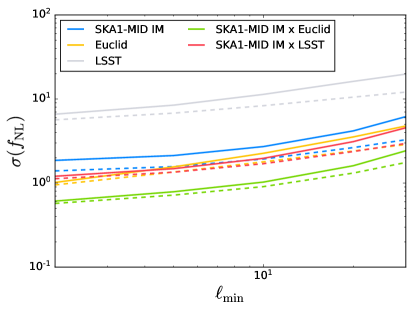
Figure 1: Marginalized uncertainties on $f_{\rm NL}$ as function of the minimum multipole $\ell_{\rm min}$ of LSS. Solid curves correspond to LSS experiments without CMB: SKA1 IM (blue), Euclid-like (yellow), LSST-like (grey), and the combinations SKA1 IM $\times$ Euclid-like (green) and LSST-like (red). Dashed lines correspond to the inclusion of CMB-S4 lensing ($\ell_{\rm min}=30$).

4.2 $f_{\rm NL},n_{\rm NL}$ model of PNG

We turn now to the constraints for the two-parameter model (2) with a running of $f_{\rm NL}$, using the same specification as in Eqs. (37)–(40). Figure 2 shows the marginalized uncertainties on the 2-dimensional $(f_{\rm NL},n_{\rm NL})$ parameter space.

The uncertainties for single tracers are

$$\sigma\left(n_{\rm NL}\right)\simeq\begin{cases}2.7&\mbox{SKA1 }(\ell_{\rm min}=5)\,,\\ 0.35&\mbox{Euclid-like }(\ell_{\rm min}=10)\,,\\ 0.37&\mbox{LSST-like }(\ell_{\rm min}=20)\,.\end{cases}$$ (42)

Including CMB lensing from CMB-S4 with $\ell_{\rm min}=30$, errors decrease to

$$\sigma\left(n_{\rm NL}\right)\simeq\begin{cases}1.4&\mbox{SKA1}\times\mbox{CMB-S4}\,,\\ 0.24&\mbox{Euclid-like}\times\mbox{CMB-S4}\,,\\ 0.32&\mbox{LSST-like}\times\mbox{CMB-S4}\,.\end{cases}$$ (43)

The combination of intensity and number counts leads to

$$\sigma\left(n_{\rm NL}\right)\simeq\begin{cases}0.13&\mbox{SKA1}\times\mbox{Euclid-like}\,,\\ 0.24&\mbox{SKA1}\times\mbox{LSST-like}\,.\end{cases}$$ (44)

When all three tracers are combined, the tightest constraint obtained is

$$\sigma\left(n_{\rm NL}\right)\simeq\begin{cases}0.12&\mbox{SKA1}\times\mbox{Euclid-like}\times\mbox{CMB-S4}\,,\\ 0.22&\mbox{SKA1}\times\mbox{LSST-like}\times\mbox{CMB-S4}\,.\end{cases}$$ (45)

In this case the uncertainties on $f_{\rm NL}$ degrade by $\sim 20\%$ on average, compared to the case without running, which shows a weak degeneracy between the two parameters.

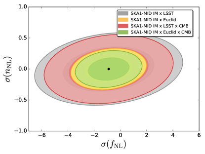
Figure 2: Marginalized 2-dimensional contours (68% and 95% CL) for $f_{\rm NL}$ and $n_{\rm NL}$, with $\ell_{\rm min}=$ 5, 10, 30 for HI IM, galaxy number counts, and CMB respectively. The multi-tracer combinations are: SKA1 $\times$ Euclid-like (yellow), SKA1 $\times$ LSST-like (grey), CMB $\times$ SKA1 $\times$ Euclid-like (green), and CMB $\times$ SKA1 $\times$ LSST-like (red).

4.3 Comparison with other results on $\sigma\left(f_{\rm NL}\right)$

In this work, we consistently make use of the CMB convention to define $f_{\rm NL}$. In comparison with other work where the alternative LSS convention is used, we quote here the relevant constraints modified to be consistent with the CMB convention (19).

In Alonso et al. (2015) and Alonso & Ferreira (2015), the case of LSST-like and SKA1-MID IM is treated (without using CMB-S4), giving uncertainties down to $\sim 0.31$ for the multi-tracer case. They use a greater number of thinner bins for the SKAI-MID IM survey, i.e., 100 bins with equal co-moving width, while we use 27 such bins. For the LSST-like survey, they use 9 bins with widths chosen to ensure equal source density, as opposed to our 10 fixed-width bins. They use a multipole range $2\leq\ell\leq 500$ for both tracers, and assume larger sky fractions: 0.5 for LSST-like and 0.75 for SKA1, with the overlap taken as 0.4, which also exceeds ours. Their LSST-like redshift distribution has a slightly more pessimistic 40 sources/arcmin², versus our 48 sources/arcmin² according to Alonso et al. (2018), which results in a slightly lower shot noise. In summary, their greater sky area and smaller $\ell_{\rm min}$ are the main reasons for their more optimistic constraints.

In Fonseca et al. (2015) there is a multi-tracer analysis for Euclid-like and SKA1-MID IM surveys. Their results give $0.72\leq\sigma\left(f_{\rm NL}\right)\leq 1.05$, depending on (a) the maximum multipole chosen ($\ell_{\rm max}=60$ or $\ell_{\rm max}=300$), and (b) the sky overlap (50% or 100%). Their multipole range for all tracers extends down to $\ell_{\rm min}=2$. They also consider a LSST-like survey with sky area equal to that of the entire SKA1-MID IM. They obtain the multi-tracer result $\sigma\left(f_{\rm NL}\right)\simeq 0.61$ for $\ell_{\rm max}=300$, which is lower than ours. Considering that the effect of $f_{\rm NL}$ is captured only on larger scales, this difference in $\ell_{\rm max}$ should have a negligible effect on the final uncertainties. The sky fraction in their 50% overlap case is 0.18, which is smaller than our shared sky fraction of 0.36 for SKA1-MID IM and Euclid-like. However, their assumed SKA1 sky fraction is 0.72, which is larger than our 0.48, which follows Bacon et al. (2018). Their LSST-like sky fraction is also chosen as 0.72, larger than our sky fraction for LSST-like of $\sim 0.33$, according to Alonso et al. (2018). The bias fitting functions used are the same as ours, and the same kind of nuisance parameters are introduced. The main driver of the difference in results from ours is again the greater sky area and smaller $\ell_{\rm min}$ that they assumed.

In Schmittfull & Seljak (2018), the case of LSST-like clustering and CMB-S4 lensing in cross correlation is investigated. The uncertainties found are $\sigma\left(f_{\rm NL}\right)\simeq 0.4$ or $\sigma\left(f_{\rm NL}\right)\simeq 1.0$ for the cases where the minimum multipole for both tracers is either 2 or 20. The galaxy redshift distribution is split into 6 bins, extending over a larger redshift range $0<z<7$ and assuming 50 sources/arcmin². The sky fractions they used are 0.5 for both CMB-S4 and LSST-like, assuming 100% overlap. Their fiducial bias model is $b(z)=1+z$ as opposed to the one we use, $b(z)=0.95/D(z)$. Once again, the greater sky area and smaller $\ell_{\rm min}$ that they assumed produce more optimistic constraints than ours. The larger redshift range that they considered is not as important. If we use the assumptions made by them, we recover their results.

5 Conclusions

In this paper we have shown how up to three tracers of the cosmic density field can be used to extract precise measurements of perturbations on scales beyond the equality scale. Specifically we forecast that a conservative combination of an SKA1-MID HI intensity mapping survey with the galaxy clustering from two photometric galaxy surveys (Euclid- and LSST-like), and with CMB lensing from CMB-S4, could reach uncertainties for primordial non-Gaussianity parameters of $\sigma(f_{\rm NL})\lesssim 0.9$ and $\sigma(n_{\rm NL})\lesssim 0.2$. We highlighted the importance of CMB lensing information through the cross-correlation with intensity/ number counts to further improve the uncertainties on $f_{\rm NL}$.

The uncertainties obtained for local type PNG in the single-tracer cases are $\sigma(f_{\rm NL})\simeq 2.1$ for SKA1-MID IM with $\ell_{\rm min}=5$, $\sigma(f_{\rm NL})\simeq 2.3$ for Euclid-like with $\ell_{\rm min}=10$, and $\sigma(f_{\rm NL})\simeq 16.2$ for LSST-like with $\ell_{\rm min}=20$. On the running index of $f_{\rm NL}$ in the extended local PNG model, we found $\sigma(n_{\rm NL})\simeq 2.7$, $0.35$, $0.37$ respectively.

Combining two different large-scale structure surveys via the multi-tracer approach, we forecast $\sigma(f_{\rm NL})\simeq 0.96\ (1.6)$ for SKA1-MID IM with Euclid-like (LSST-like) and $\sigma(n_{\rm NL})\simeq 0.13\ (0.24)$.

When we combine CMB lensing information (with $\ell_{\rm min}=30$) from a possible CMB-S4 ground-based experiment in the multi-tracer, with a single LSS survey, we found that the single-tracer errors decrease to $\sigma(f_{\rm NL})\simeq 1.6$, $1.8$, $10.5$ for SKA1-HI IM, Euclid-like, and LSST-like, respectively.

When all three tracers are included in a multi-tracer analysis, the tightest uncertainties were predicted

$${\sigma(f_{\rm NL})\simeq 0.90~{}\mbox{and}~{}\sigma(n_{\rm NL})\simeq 0.12}$$

$${\mbox{for}~{}\mbox{SKA1}\times\mbox{Euclid-like}\times\mbox{CMB-S4}.}$$ (46)

Using LSST-like instead of Euclid-like, these degrade to $\sigma(f_{\rm NL})\simeq 1.4$ and $\sigma(n_{\rm NL})\simeq 0.22$.

We considered also the possibility of using simulated Planck-like data, leading to uncertainties on the cosmological parameters compatible with the latest results in Akrami et al. (2018); Aghanim et al. (2018a, b) as representative of current CMB measurements. In this case, the improvement in uncertainties by adding Planck to the single-tracer cases is very small and mostly due to parameter degeneracy with the standard cosmological parameters, rather than an imprinting of $f_{\rm NL}$ on the cross-correlation between intensity/number counts with CMB lensing. We also tested the possibility of completing the missing first multipoles $2\leq\ell_{\rm min}<30$ in the CMB spectra, but we found no further improvement.

Constraints on PNG parameters from the measurement of ultra-large scales depend strongly on the $\ell_{\rm min}$ and $f_{\rm sky}$ considered in the analysis. Our constraints use more conservative estimates and the most up-to-date specifications for the surveys involved. In light of the differences in assumptions made in previous papers, it is not unexpected that our constraints are weaker.

We assumed the minimum multipoles and sky areas for each experiment according to up-to-date specifications for each survey:
$\ell_{\rm min}=~{}\,5,\,\Omega=20,000\,$deg² – SKA1 (Bacon et al., 2018);
$\ell_{\rm min}=10,\,\Omega=15,000\,$deg² – Euclid-like (Amendola et al., 2018);
$\ell_{\rm min}=20,\,\Omega=13,800\,$deg² – LSST-like (Alonso et al., 2018);
$\ell_{\rm min}=30,\,\Omega=16,500\,$deg² – CMB-S4 (Abazajian et al., 2016).

We also studied how uncertainties change as a function of the minimum multipole, shown in Fig. 1. For the multi-tracer sky overlap area, we took the smallest of the sky fractions involved. For smaller overlaps, the uncertainties will be mildly negatively affected.

Finally, many other different tracers have been highlighted as good candidates to obtain competitive constraints on $f_{\rm NL}$, such as clusters of galaxies (Pillepich et al., 2012; Mana et al., 2013; Sartoris et al., 2016), cosmic infrared background (Tucci et al., 2016), cosmic voids (Chan et al., 2018) and different IM lines, like H$\alpha$, CO and CII (Fonseca et al., 2018; Moradinezhad Dizgah & Keating, 2019). These could also be included in the analysis in order to reach more robust and tighter constraints.

References

- Abazajian et al. (2016) Abazajian K. N., et al., 2016. (arXiv:1610.02743)
- Abramo & Bertacca (2017) Abramo L. R., Bertacca D., 2017, Phys. Rev., D96, 123535
- Abramo & Leonard (2013) Abramo L. R., Leonard K. E., 2013, Mon. Not. Roy. Astron. Soc., 432, 318
- Acquaviva et al. (2003) Acquaviva V., Bartolo N., Matarrese S., Riotto A., 2003, Nucl. Phys., B667, 119
- Aghanim et al. (2018a) Aghanim N., et al., 2018a. (arXiv:1807.06209)
- Aghanim et al. (2018b) Aghanim N., et al., 2018b. (arXiv:1807.06210)
- Akrami et al. (2018) Akrami Y., et al., 2018. (arXiv:1807.06205)
- Akrami et al. (2019) Akrami Y., et al., 2019. (arXiv:1905.05697)
- Albrecht & Steinhardt (1982) Albrecht A., Steinhardt P. J., 1982, Phys. Rev. Lett., 48, 1220
- Alonso & Ferreira (2015) Alonso D., Ferreira P. G., 2015, Phys. Rev., D92, 063525
- Alonso et al. (2015) Alonso D., Bull P., Ferreira P. G., Maartens R., Santos M., 2015, Astrophys. J., 814, 145
- Alonso et al. (2018) Alonso D., et al., 2018. (arXiv:1809.01669)
- Amendola et al. (2018) Amendola L., et al., 2018, Living Rev. Rel., 21, 2
- Bacon et al. (2018) Bacon D. J., et al., 2018. (arXiv:1811.02743)
- Ballardini & Maartens (2019) Ballardini M., Maartens R., 2019, Mon. Not. Roy. Astron. Soc., 485, 1339
- Ballardini et al. (2016) Ballardini M., Finelli F., Fedeli C., Moscardini L., 2016, JCAP, 1610, 041
- Bartolo et al. (2004) Bartolo N., Komatsu E., Matarrese S., Riotto A., 2004, Phys. Rept., 402, 103
- Battye et al. (2004) Battye R. A., Davies R. D., Weller J., 2004, Mon. Not. Roy. Astron. Soc., 355, 1339
- Becker & Huterer (2012) Becker A., Huterer D., 2012, Phys. Rev. Lett., 109, 121302
- Biagetti et al. (2017) Biagetti M., Lazeyras T., Baldauf T., Desjacques V., Schmidt F., 2017, Mon. Not. Roy. Astron. Soc., 468, 3277
- Bull et al. (2015) Bull P., Ferreira P. G., Patel P., Santos M. G., 2015, Astrophys. J., 803, 21
- Byrnes & Choi (2010) Byrnes C. T., Choi K.-Y., 2010, Adv. Astron., 2010, 724525
- Byrnes et al. (2009) Byrnes C. T., Choi K.-Y., Hall L. M. H., 2009, JCAP, 0902, 017
- Byrnes et al. (2010) Byrnes C. T., Nurmi S., Tasinato G., Wands D., 2010, JCAP, 1002, 034
- Camera et al. (2013) Camera S., Santos M. G., Ferreira P. G., Ferramacho L., 2013, Phys. Rev. Lett., 111, 171302
- Castorina et al. (2019) Castorina E., et al., 2019. (arXiv:1904.08859)
- Challinor & Lewis (2011) Challinor A., Lewis A., 2011, Phys. Rev., D84, 043516
- Chan et al. (2018) Chan K. C., Hamaus N., Biagetti M., 2018. (arXiv:1812.04024)
- Chang et al. (2008) Chang T.-C., Pen U.-L., Peterson J. B., McDonald P., 2008, Phys. Rev. Lett., 100, 091303
- Chen (2005) Chen X., 2005, Phys. Rev., D72, 123518
- Chen (2010) Chen X., 2010, Adv. Astron., 2010, 638979
- Chen et al. (2015) Chen X., Namjoo M. H., Wang Y., 2015, JCAP, 1502, 027
- Creminelli & Zaldarriaga (2004) Creminelli P., Zaldarriaga M., 2004, JCAP, 0410, 006
- Cunnington et al. (2019) Cunnington S., Wolz L., Pourtsidou A., Bacon D., 2019
- Dalal et al. (2008) Dalal N., Doré O., Huterer D., Shirokov A., 2008, Phys. Rev., D77, 123514
- Desjacques et al. (2009) Desjacques V., Seljak U., Iliev I., 2009, Mon. Not. Roy. Astron. Soc., 396, 85
- Desjacques et al. (2018) Desjacques V., Jeong D., Schmidt F., 2018, Phys. Rept., 733, 1
- Ferramacho et al. (2014) Ferramacho L. D., Santos M. G., Jarvis M. J., Camera S., 2014, Mon. Not. Roy. Astron. Soc., 442, 2511
- Ferraro & Smith (2015) Ferraro S., Smith K. M., 2015, Phys. Rev., D91, 043506
- Fonseca et al. (2015) Fonseca J., Camera S., Santos M., Maartens R., 2015, Astrophys. J., 812, L22
- Fonseca et al. (2017) Fonseca J., Maartens R., Santos M. G., 2017, Mon. Not. Roy. Astron. Soc., 466, 2780
- Fonseca et al. (2018) Fonseca J., Maartens R., Santos M. G., 2018, Mon. Not. Roy. Astron. Soc., 479, 3490
- Gangui et al. (1994) Gangui A., Lucchin F., Matarrese S., Mollerach S., 1994, Astrophys. J., 430, 447
- Giusarma et al. (2018) Giusarma E., Vagnozzi S., Ho S., Ferraro S., Freese K., Kamen-Rubio R., Luk K.-B., 2018, Phys. Rev., D98, 123526
- Guth (1981) Guth A. H., 1981, Phys. Rev., D23, 347
- Hawking et al. (1982) Hawking S. W., Moss I. G., Stewart J. M., 1982, Phys. Rev., D26, 2681
- Hirata & Seljak (2003) Hirata C. M., Seljak U., 2003, Phys. Rev., D68, 083002
- Howlett et al. (2012) Howlett C., Lewis A., Hall A., Challinor A., 2012, JCAP, 1204, 027
- Hu & Okamoto (2002) Hu W., Okamoto T., 2002, Astrophys. J., 574, 566
- Hu & White (1997) Hu W., White M. J., 1997, Phys. Rev., D56, 596
- Knox (1995) Knox L., 1995, Phys. Rev., D52, 4307
- Kovetz et al. (2017) Kovetz E. D., et al., 2017. (arXiv:1709.09066)
- Laureijs et al. (2011) Laureijs R., et al., 2011. (arXiv:1110.3193)
- Lewis et al. (2000) Lewis A., Challinor A., Lasenby A., 2000, Astrophys. J., 538, 473
- Li et al. (2018) Li X., Weaverdyck N., Adhikari S., Huterer D., Muir J., Wu H.-Y., 2018, Astrophys. J., 862, 137
- Linde (1982) Linde A. D., 1982, Phys. Lett., 108B, 389
- Linde (1983) Linde A. D., 1983, Phys. Lett., 129B, 177
- LoVerde et al. (2008) LoVerde M., Miller A., Shandera S., Verde L., 2008, JCAP, 0804, 014
- Ma et al. (2005) Ma Z.-M., Hu W., Huterer D., 2005, Astrophys. J., 636, 21
- Maldacena (2003) Maldacena J. M., 2003, JHEP, 05, 013
- Mana et al. (2013) Mana A., Giannantonio T., Weller J., Hoyle B., Huetsi G., Sartoris B., 2013, Mon. Not. Roy. Astron. Soc., 434, 684
- Matarrese & Verde (2008) Matarrese S., Verde L., 2008, Astrophys. J., 677, L77
- Mifsud & van de Bruck (2019) Mifsud J., van de Bruck C., 2019
- Mo & White (1996) Mo H. J., White S. D. M., 1996, Mon. Not. Roy. Astron. Soc., 282, 347
- Moradinezhad Dizgah & Keating (2019) Moradinezhad Dizgah A., Keating G. K., 2019, Astrophys. J., 872, 126
- Muñoz et al. (2017) Muñoz J. B., Kovetz E. D., Raccanelli A., Kamionkowski M., Silk J., 2017, JCAP, 1705, 032
- Mukhanov & Chibisov (1981) Mukhanov V. F., Chibisov G. V., 1981, JETP Lett., 33, 532
- Oppizzi et al. (2018) Oppizzi F., Liguori M., Renzi A., Arroja F., Bartolo N., 2018, JCAP, 1805, 045
- Pillepich et al. (2012) Pillepich A., Porciani C., Reiprich T. H., 2012, Mon. Not. Roy. Astron. Soc., 422, 44
- Raccanelli et al. (2015) Raccanelli A., Dore O., Dalal N., 2015, JCAP, 1508, 034
- Salopek & Bond (1990) Salopek D. S., Bond J. R., 1990, Phys. Rev., D42, 3936
- Santos et al. (2015) Santos M., et al., 2015, in Proceedings, Advancing Astrophysics with the Square Kilometre Array (AASKA14): Giardini Naxos, Italy, June 9-13, 2014. p. 019, doi:10.22323/1.215.0019
- Santos et al. (2017) Santos M. G., et al., 2017, in Proceedings, MeerKAT Science: On the Pathway to the SKA (MeerKAT2016): Stellenbosch, South Africa, May 25-27, 2016. (arXiv:1709.06099)
- Sartoris et al. (2016) Sartoris B., et al., 2016, Mon. Not. Roy. Astron. Soc., 459, 1764
- Sato (1981) Sato K., 1981, Mon. Not. Roy. Astron. Soc., 195, 467
- Schmidt & Kamionkowski (2010) Schmidt F., Kamionkowski M., 2010, Phys. Rev., D82, 103002
- Schmittfull & Seljak (2018) Schmittfull M., Seljak U., 2018, Phys. Rev., D97, 123540
- Sefusatti et al. (2009) Sefusatti E., Liguori M., Yadav A. P. S., Jackson M. G., Pajer E., 2009, JCAP, 0912, 022
- Seljak (2009) Seljak U., 2009, Phys. Rev. Lett., 102, 021302
- Sheth & Tormen (1999) Sheth R. K., Tormen G., 1999, Mon. Not. Roy. Astron. Soc., 308, 119
- Slosar et al. (2008) Slosar A., Hirata C., Seljak U., Ho S., Padmanabhan N., 2008, JCAP, 0808, 031
- Smith et al. (2012) Smith K. M., Hanson D., LoVerde M., Hirata C. M., Zahn O., 2012, JCAP, 1206, 014
- Starobinsky (1980) Starobinsky A. A., 1980, Phys. Lett., B91, 99
- Tucci et al. (2016) Tucci M., Desjacques V., Kunz M., 2016, Mon. Not. Roy. Astron. Soc., 463, 2046
- Witzemann et al. (2019) Witzemann A., Alonso D., Fonseca J., Santos M. G., 2019, Mon. Not. Roy. Astron. Soc., 485, 5519
- Wyithe & Loeb (2008) Wyithe S., Loeb A., 2008, Mon. Not. Roy. Astron. Soc., 383, 606
- Yamauchi et al. (2014) Yamauchi D., Takahashi K., Oguri M., 2014, Phys. Rev., D90, 083520
- Yoo et al. (2012) Yoo J., Hamaus N., Seljak U., Zaldarriaga M., 2012, Phys. Rev., D86, 063514
- de Putter & Doré (2017) de Putter R., Doré O., 2017, Phys. Rev., D95, 123513